Regularized Stein Variational Gradient Flow
Abstract.
The Stein Variational Gradient Descent (SVGD) algorithm is an deterministic particle method for sampling. However, a mean-field analysis reveals that the gradient flow corresponding to the SVGD algorithm (i.e., the Stein Variational Gradient Flow) only provides a constant-order approximation to the Wasserstein Gradient Flow corresponding to the KL-divergence minimization. In this work, we propose the Regularized Stein Variational Gradient Flow which interpolates between the Stein Variational Gradient Flow and the Wasserstein Gradient Flow. We establish various theoretical properties of the Regularized Stein Variational Gradient Flow (and its time-discretization) including convergence to equilibrium, existence and uniqueness of weak solutions, and stability of the solutions. We provide preliminary numerical evidence of the improved performance offered by the regularization.
1. Introduction
Given a potential function , the sampling problem involves generating samples from the density
| (1) |
being the normalization constant, which is typically assumed to be unknown or hard to compute. The task of sampling arises in several fields of applied mathematics including Bayesian statistics and machine learning in the context of numerical integration. There are two widely-used approaches for sampling: (i) diffusion-based randomized algorithms, which are based on discretizations of certain diffusion processes, and (ii) particle-based deterministic algorithms, which are discretizations of certain approximate gradient flows. A central idea connecting the two approaches is the seminal work by [JKO98] which provided a variational interpretation of the Langevin diffusion as the Wasserstein Gradient Flow (WGF),
| (2) |
where the term could be interpreted as the Wasserstein gradient111See, for example, [AGS05, San17] for the exact definition. of the relative entropy functional (also called as the Kullback–Leibler divergence), defined by s
evaluated at . This leads to the idea that sampling could be viewed as optimization on the space of measures, a viewpoint that has provided a deeper understanding of the sampling problem [Wib18, TSA20].
There are several merits and disadvantages to both the randomized and deterministic discretization of the (approximate) WGF. First, note that obtaining exact space-time discretization of the WGF in (2) is not possible. Indeed, due to the presence of the diffusion term, when initialized with an -particle based empirical measure, the particles do not remain as particles for any time . Hence, on the one hand, randomized discretizations like the Langevin Monte Carlo algorithm, are used as implementable space-time discretizations of the WGF. On the other hand, motivated by applications where the randomness in the discretization is undesirable, in the applied mathematics literature, other discretizations of approximate WGF were developed. Such methods are predominantly based on using mollifiers and we refer the reader to [Rav85, Rus90, DM90, CB16, CCP19] for a partial list and to [Che17], for a comprehensive overview.
Recently, in the machine learning community, the Stein Variational Gradient Descent [LW16, Liu17] was proposed as another deterministic discretization of approximate WGF, and has gathered significant attention due to applications to reinforcement learning [LRLP17], graphical modeling [WZL18], measure quantization [XKS22], and other fields of machine learning and applied mathematics [WTBL19, CLGL+20, CLGL+20, KSA+20]. Due to the use of the reproducing kernels, the Stein Variational Gradient Descent (SVGD) algorithm provides a space-time discretization of the following approximate Wasserstein Gradient Flow (which we refer to as the Stein Variational Gradient Flow (SVGF) for simplicity)
| (3) |
where is the integral operator defined as for a function , and for a kernel ; see, for example [LLN19]. Hence, SVGD (which is based on the SVGF), in this context, while being deterministic only provides a discretization of a constant-order approximation to the Wasserstein Gradient Flow due to the presence of the kernel integral operator. Indeed, if and is bounded continuous translation invariant characteristic kernel [SGF+10] on (e.g., Gaussian, Laplacian kernels), then
where . This shows that the order of the error is crucially dependent on the choice of the kernel .
To overcome the above issue with the SVGF, in this work, we propose the Regularized Stein Variational Gradient Flow (R-SVGF). To motivate the proposed flow, we first note that the Wasserstein gradient lives in , while the kernelized Wasserstein gradient morally lives in . If , then it is easy to verify that
Additionally, if is sufficiently smooth, i.e., there exists such that , for some (see, for example, [CZ07]), then
In other words, is a good approximation to for small . With this motivation, we propose the following R-SVGF given by
| (4) |
for some regularization parameter , where R-SVGF arbitrarily approximates the WGF as . It is important to note that in the case of , we have , yet, (3) suffers from the drawback of providing only a constant-order approximation to (2).
1.1. Summary of Contributions
Our contributions in this work are as follows:
-
(1)
We propose the Regularized SVGF (R-SVGF) that interpolates between the Wasserstein Gradient Flow and the SVGF. The advantage of the proposed flow is that one could obtain an implementable space-time discretization as long as the regularization parameter is bounded away from zero. The main intuition behind the proposed flow is to pick an appropriately small choice of regularization parameter so that we could arbitrarily approximate the WGF (Theorems 1 and 3).
-
(2)
For the R-SVGF, we provide rates of convergence to the equilibrium density in two cases: (i) in the Fisher Information metric under no assumptions on the target (Theorem 2) and (ii) in the KL-divergence metric under an LSI assumption on the target (Theorem 4). We also establish similar results for the time-discretized R-SVGF (Theorems 5 and 6).
- (3)
-
(4)
We provide preliminary numerical experiments demonstrating the advantage of the space-time discretization of the R-SVGF, which we call as the the Regularized Stein Variational Gradient Descent (R-SVGD) algorithm, over the standard SVGD algorithm.
1.2. Organization
The rest of the paper is organized as follows. In Section 1.3, we introduce the notations used in the rest of the paper. In Section 2, we provide the preliminaries on reproducing kernel Hilbert spaces required for our work. In Section 3, we introduce the R-SVGF, along with the notion of regularized Stein-Fisher information, required for our analysis. Due to the technical nature of the proofs, we postpone the results on existence and uniqueness of the R-SVGF, and related stability results respectively to Sections 5 and 6. In Section 4, we provide convergence results on the R-SVGF flow and its time-discretized version. We conclude in Section 7 with a space-time discretization which provides a practically implementable algorithm, and provide preliminary empirical results.
1.3. Notations
We use the following notations throughout this work:
-
•
For a matrix, denotes the matrix 2-norm (spectral norm) and denotes the Hilbert-Schmidt norm which is defined as for any matrix .
-
•
The term denotes the identity matrix. corresponds to the identity operator in the RKHS. corresponds to the identity operator in .
-
•
denotes the space of all probability measures on , and denotes the space of all probability measures on with finite second moments.
-
•
denotes the space of all essentially bounded measurable functions on with for any .
-
•
For any , is the space of all -square integrable measurable function on with .
-
•
Let and denote two function spaces. For an operator , we denote the adjoint operator of by . We denote the operator norm by , which is defined as . When we don’t emphasize the spaces, we denote the operator norm of by for simplicity.
-
•
Let and denote two Hilbert spaces. For an operator , we denote the Hilbert-Schmidt norm by which is defined as where is an orthonormal basis of . We denote the nuclear norm by which is defined as where is an orthonormal basis of .
-
•
For a smooth function , denotes the gradient of in the first variable and denotes the gradient of in the second variable.
-
•
For a map , denotes the -th component of the function value and denotes the Jacobian, i.e., .
-
•
represents the push-forward of the density under a map .
-
•
denotes inner-product in the Hilbert space . denotes inner-product in the Euclidean space .
-
•
is the space of all -valued continuous functions on .
-
•
For any function space on , is the space of functions such that for any fixed , and for any fixed , is a continuous function on . is the space of functions such that for any fixed , and for any fixed , is a continuous function with continuous first order derivative on .
-
•
is the space of all measurable functions on that vanish at infinity, i.e., for any , as and as .
-
•
Suppose is a vector-valued function. For a function space , we say if such that for all .
2. Preliminaries on Reproducing Kernel Hilbert Space
In this section, we introduce some properties of RKHS which would be used later in the formulation and analysis of R-SVGF. We refer the reader to [SC08, BTA11, PR16] for the basics of RKHS. We let to be a separable RKHS over with the reproducing kernel and with denoting the associated RKHS norm. We make the following assumption on the kernel function throughout the paper.
Assumption A1.
The kernel function is strictly positive definite, continuous and bounded.
The following results are essentially based on [SC08, Lemma 4.23, and Theorems 4.26 and 4.27].
Proposition 1 ([SC08]).
Under Assumption A1, the following holds.
-
(i)
The kernel function is bounded if and only if every is bounded. Moreover, the inclusion is continuous and , where .
-
(ii)
Let be a -finite measure on . Assume that
Then consists of -integrable functions and the inclusion is continuous with . Moreover, the adjoint of this inclusion is the operator defined by
-
(iii)
is dense in if and only if is injective. Alternatively, has a dense image if and only if is injective.
-
(iv)
is a Hilbert-Schmidt operator with . Moreover, the integral operator is compact, positive, self-adjoint, and nuclear with .
The RKHS norm of is given by . The norm of is given by . When with and , we define as a vector in and for all . When with and , we define as a vector in and for all . Note also that . We refer the interested reader to [CZ07] for more details.
Finally, we remark that by letting to be the set of eigenvalues and eigenfunctions of the operator where and form an orthonormal system in , we have the following spectral representation that, for all ,
| (5) |
Computing the spectral representation, in general for any given and kernel is a non-trivial task. Results are only known on a case-by-case basis; see, for example, [MNY06, AM14, CX20, SH21]. However, we use the decomposition only in our analysis. For the purely practical algorithm that we describe eventually in Section 7, we do not need to know the decomposition explicitly.
3. Regularized SVGF
We now introduce the formulation of the Regularized-SVGF and discuss its connection with SVGF and the WGF. Recall that in the mean-field limit, the SVGF in (3) only provides a constant order approximation to the WGF in (2), due to the presence of the operator . As the operator is not invertible, we seek to obtain a regularized inverse so that we end up with the following Regularized-SVGF, as in (4), for some regularization parameter . Note in particular that as , the Regularized-SVGF gets arbitrarily close to the WGF. Our goal in this section is to derive the above mentioned R-SVGF from first principles.
The central operator required in our formulation is the following Stein operator, which is defined for all , and for all smooth maps , as
where denotes the outer-product. Now, the Wasserstein Gradient Flow in (2) could be thought of as follows. Consider moving a particle (for some ) based on the mapping , where is a step-size parameter, and is a vector-field chosen so that the KL-divergence between the pushforward of according to , denoted as , and the target density in minimal. Liu and Wang [LW16, Theorem 3.1], showed that
We also refer to [JKO98] for an earlier version of the same result. Based on this observation, if we try to find the vector-field in the unit-ball of that maximizes the quantity , a straight-forward calculation based on integration-by-parts, results in the optimal being the Wasserstein gradient . To have a practical implementation, [LW16] considered maximizing over the unit-ball in the RKHS , which results in the optimal vector-field being equal to , and correspondingly results in the SVGF in (3).
In this work, we propose to find the vector field that maximizes over the unit-ball with respect to an interpolated norm between and . Specifically, the interpolation norm that we consider is of the form , for some regularization parameter , which trades-off between and . We also remark here that a similar idea has been leveraged in the context of RKHS-based statistical hypothesis testing [BLY21]. Formally, for , we consider the following optimization problem.
For any , the optimal vector field, that minimizes can be described via the following result.
Proposition 2.
Let and be the density of when , for some density . For , define
Then the direction of steepest descent in that maximizes is given by
where is the inclusion operator and is its adjoint as in Proposition 1. Furthermore, under the optimal vector field , we have .
Proof.
First note that according to [LW16, Theorem 3.1], we have
Therefore, we have
Next, observe that we have
Meanwhile, the constraint can be written as
where is the identity operator. Now, note that is well-defined since is positive, compact and self-adjoint. Therefore based on the above display, the constraint is equivalent to
Since the spectrum of is positive and , is invertible. For all , there exists a unique such that . Applying this fact along with the equivalent form of the constraint, we have
where the second identity follows from the fact that is self-adjoint and the upper bound in the last inequality is achieved when
and the result hence follows. ∎
With the optimal-vector field as derived above, we consider the following mean-field partial differential equation (PDE) as the R-SVGF:
| (6) |
It is important to notice that the R-SVGF interpolates between SVGF and WGF. However, the regime of interest for us is when , as we get arbitrarily close to the WGF. We quantify this statement precisely in the later sections. On the other hand, when R-SVGF becomes the SVGF.
Remark 1.
We now make the following remarks about the above result.
- (i)
-
(ii)
The operator in (6) has an equivalent expression as we discuss below. First, we claim that
To see that, we start with the trivial identity in the first line below and proceed as
According to this observation, (6) can also be written in the following form
thereby providing the R-SVGF introduced in (4) in Section 1.
-
(iii)
Particle-based spatial discretization. We now describe the spatial discretization of the R-SVGF. Based on the results in Proposition 2 and Remark 1, we obtain the following ODE system:
where is the set of particles. is the empirical distribution at time , provides a -particle spatial discretization of the R-SVGF.
-
(iv)
Time discretization. We also have the following time-discretization of the R-SVGF. Let be the sequence of time step-size. We denote the density at the -th iterate by for all integers . Then the time discretization of the R-SVGF can be written as
(7) where .
-
(v)
The parameter can also be made to be dependent on or ; in fact, in our analysis we pick a time-varying regularization parameter.
4. Convergence Results in Continuous and Discrete Time
Our goal in this section is derive convergence guarantees for the R-SVGF. Before we proceed, we introduce the notion of Regularized Stein-Fisher information (or Regularized Kernel Stein Discrepancy).
4.1. Regularized Stein-Fisher Information and its Properties
Note that several works, for example [KSA+20, DNS19, SSR22], used the notion of Stein-Fisher Information to understand the convergence properties of the SVGD algorithm. The Stein-Fisher information was introduced in [CSG16, LLJ16, GM17] under the name Kernel Stein Discrepancy. However, a drawback of the Stein-Fisher information is that it is a weaker metric, for example in comparison to the Fisher information metric; see [GM17, GDVM19, SGBSM20]. Below, we introduce a regularized version of the Stein-Fisher information and show that as the regularization parameter tends to zero, it converges to the standard Fisher information.
Let , then, the Fisher information corresponds to
with being an orthonormal basis to . Correspondingly, the Stein-Fisher information is defined as
where are the set of eigenvalues and eigenvectors of the operator , with .
Remark 2.
Strictly speaking, the above notation implicitly assumes that the operator has a trivial null space, in which case the and hence the eigenfunctions form an orthonormal basis to . However, our analysis does not require this condition on . In particular, if has a non-trivial null-space, then . In this case, our analysis still holds true. For example, with a slight abuse of notation, if we let , for certain values of , to also denote the basis of the null-space of , conclusions similar to our results hold.
With this representation for the Fisher information and the Stein-Fisher information, it is immediately clear that the Stein-Fisher information is severely restrictive, in particular when the eigenvalues of the chosen RKHS decay faster. To counter this effect, we introduce the following regularized Stein-Fisher information and show that when the regularization parameter is chosen appropriately, the regularized Stein-Fisher information upper and lower bounds Fisher information.
Definition 1 (Regularized Stein-Fisher Information).
For any probability measure , the regularized Stein Fisher information from to , denoted as , is defined as
| (8) |
The regularized Stein Fisher information in (8) is well-defined because the operator
is positive and for any , if and only if .
Remark 3.
The regularized Stein Fisher information has the following alternative representation:
| (9) |
For , with the fact that decreases to zero as , the regularized Stein Fisher information and the Stein Fisher information both encode the spectral decay information of . However, note that the regularized Stein Fisher information tends to the Fisher information as . Hypothetically speaking, if is set to zero, then the regularized Stein Fisher information actually becomes the Fisher information. In our analysis, we will take advantage of the relation between the regularized Stein Fisher information and the Fisher information, while studying the convergence properties of R-SVGF under Log-Sobolev inequality assumptions on the target . A precise relation between the regularized Stein Fisher information and the Fisher information is stated in the following result. Before stating the result, we introduce the following notation for convenience. For , we denote the pre-image of under as
Note that is finite if and only if .
Proposition 3 (Equivalence relation between and ).
Let be a probability measure in such that and are well-defined. Suppose there exists such that If the regularization parameter is chosen to satisfy the following condition,
| (10) |
then we have that
4.2. Convergence results for R-SVGF
4.2.1. Relationship between R-SVGF and WGF
We now provide the relationship between the R-SVGF and the WGF in various metrics. We first start with the relationship in the Fisher information metric, without any stringent assumptions on the target distribution (thereby allowing for multi-modal and complex densities that arise in practice). Note that the Fisher information metric corresponds to the first-order stationarity metric for the WGF obtained by minimizing the KL divergence. This metric has been recently proposed as a meaningful metric to consider in the case of sampling from general non-log-concave densities in [BCE+22]. Note in particular under mild conditions on (e.g., connected support) that having the Fisher information implies . However, even when , for some , we have that the modes of the two densities are well-aligned, as argued in [BCE+22].
Theorem 1 (Relation to the WGF in Relative Fisher Information).
Let be the solution to (6) and be the solution to the WGF, i.e.,
| (12) |
For any , suppose there exists such that Then, for any initial distribution , and for any , we have
| (13) |
Proof of Theorem 1.
First note that we have the following upper bound on :
In the above calculation, the fourth equality follows by integration-by-parts, the inequality follows by Young’s inequality for the inner product (i.e., for any ) and the last equality follows from the proof of Proposition 3. Since for some with , we obtain
where the last inequality follows from the fact that . Integrating from to , we get
Since KL-divergence is non-negative, (13) is proved. ∎
Remark 4.
The above result shows that as long as , i.e., both the WGF and R-SVGF are initialized with the same density, and is chosen such that , the averaged Fisher information along the path tends to zero. This shows the benefit of regularizing the SVGF – it enables one to closely approximate the WGF with appropriate choice of the regularization parameters.
4.2.2. Convergence to Equilibrium along the Fisher Information
We now provide results on the convergence to equilibrium along the Fisher information for the R-SVGF. We re-emphasize here that our result below is provided without any assumptions on the target .
Theorem 2 (Convergence of Fisher information).
Let be the solution to (6). For any , supppose there exists such that Then
Furthermore, if , then we get as .
Before proving the above theorem, we introduce a few intermediate results.
Proposition 4 (Decay of the KL-divergence).
Proof of Proposition 4.
We now provide the proof of Theorem 2.
Proof of Theorem 2.
From Proposition 4 and (11), we know that
where for some with . Therefore we have,
The result follows by integrating over and noting that the KL-divergence is non-negative. Now, with denoting the solution to (9), we have that is non-negative and continuous in . The claim of convergence holds because for a continuous function , if we have that , then we have as . ∎
4.2.3. Convergence in KL-divergence under LSI
While the previous result was provided without any further assumptions on the target density , in this section, we provide improved convergence results of the R-SVGF under the assumption that the satisfies the Log-Sobolev Inequality. Recall that we say that satisfies the Log-Sobolev inequality with constant if for all :
Our first result below is a stronger version of the result in Theorem 1, under the assumption that the target satisfies LSI and Assumption 1 on the initialization of the WGF.
Assumption 1.
The initial density is chosen so that the solution to (12) also satisfies LSI with parameter , for all .
Under the stronger assumption that the target density is strongly log-concave, following the arguments in [VW19, Theorem 8], it is easy to show that Assumption 1 is satisfied as long as is chosen such that it satisfies LSI. We conjecture that the same holds true even when the target density satisfies LSI and additional mild smoothnes assumptions (i.e., LSI is preserved along the trajectory as long as the initial density satisfies LSI, presumably with additional milder assumptions). However, a proof of this conjecture has eluded us thus far.
Theorem 3 (Relation to the WGF under LSI).
Proof of Theorem 3.
Our second result is a stronger version of the result in Theorem 2, under the assumption that the target distribution satisfies LSI. We remark that convergence to equilibrium of the related WGF under various functional inequalities is a well-studied topic. We refer the interested reader to [BGL14] for a detailed overview.
Theorem 4 (Decay of KL-divergence under LSI).
Assume that satisfies the log-Sobolev inequality with . Let be the solution to (6). For any , suppose there exists such that Then, for any , we have
Proof of Theorem 4.
From the proof of Theorem 2, we have
where the last inequality follows the log-Sobolev inequality. The final statement follows from Gronwall’s inequality. ∎
Remark 5 (Exponential Decay of KL-divergence).
Yet another way to state the above result is via the introducing the following regularized Stein-LSI, similar to the introduction of Stein-LSI in [DNS19]. However, the introduction of Stein-LSI is quite restrictive in the sense that it couples assumptions on the target and the chosen RKHS. This makes verifying the conditions more delicate. To counter this effect, we now introduce the notion of Regularized Stein-LSI. We say that satisfies the regularized Stein log-Sobolev inequality with constant if for all :
| (17) |
An advantage of the above condition is that, as the regularized Stein-LSI inequality becomes equivalent to the standard LSI inequality. Under the condition that the target density satisfies (17), and letting be the solution to (6), it holds that
| (18) |
The proof of (18) follows immediately from Proposition 4 and (17).
4.3. Convergence results for Time-discretized R-SVGF
In this section we analyze the convergence properties of the time-discretized R-SVGF in (7). To do so, we require the following additional assumptions.
Assumption A2.
The following conditions hold:
-
(1)
There exists a constant such that for all .
-
(2)
The potential function is twice continuously differentiable and gradient Lipschitz with parameter .
-
(3)
Along the population limit (7), for all fixed .
The smoothness assumptions in points (1) and (2) of Assumption A2 are commonly required in analyzing any discrete-time algorithms, albeit deterministic [KSA+20, SSR22] or randomized [VW19, CEL+21, BCE+22]. While it could be relaxed (see, for example, [SR22]), in general it is impossible to completely avoid them as in the case of analyzing the corresponding flows. Before stating our results, we also introduce some convenient notations. We let
where the sequences corresponds to the positive eigenvalues of the operator in the order of decreasing values.
Theorem 5 (Convergence in Fisher Divergence).
Before proving Theorem 5, we first prove the following intermediate result.
Lemma 1.
For each , define . Under the conditions in Theorem 5, we have that, for any and ,
Proof of Lemma 1.
Since for each , there exists and a function such that , where is the -th component of the function value of , we have
In the above, the first inequality follows from Cauchy-Schwartz inequality, the second inequality follows from the fact that
and the last inequality follows from Assumption A2. Meanwhile, since for all , we have for every ,
where the last inequality follows from (19). ∎
Proof of Theorem 5.
We start from studying the single step along (7). In the following analysis, for each , we denote , for all , and . Therefore we have
The following analysis is motivated by [SSR22, Proposition 3.1]. According to [Vil21, Theorem 5.34], the velocity field ruling the evolution of is and . Define , according to the chain rule in [Vil21, section 8.2],
where is the Wasserstein Hessian of at . For any and any in the Wasserstein tangent space at , the Wasserstein Hessian is given by
Therefore we can expand the difference in KL-divergence between the two consecutive iterations as
| (21) |
The first term on the right hand side of (4.3) can be studied via the spectrum of the operator .
Since , for any function we have . Hence, for the second term on the right side of (4.3), we obtain
where the last inequality follows from Assumption A2-(2). Therefore we obtain
where
with being the sequence of eigenvalues and eigenvectors to the operator such that and is an orthonormal basis of . According to Lemma 1 and Assumption A2,
and furthermore according to Lemma 1, . Therefore we get
where the last inequality follows from (19) and the second inequality follows from the fact that
which is proved in Proposition 3. Lastly, summing over and we obtain
where the last inequality follows from the fact that KL divergence is non-negative. Therefore (20) is proved. ∎
Remark 6.
We emphasize that the above result does not make any assumptions on the target density , except for the Lipschitz gradient assumption. In particular, it holds for multi-modal densities. However, the metric of convergence is the weaker Fisher information metric.
We now provide a stronger result under LSI assumptions.
Theorem 6.
Suppose Assumption A2 holds and satisfies the log-Sobolev inequality with parameter . Let be as described in (7) with initial condition such that . Assume the regularization parameter and the step-size parameters are chosen such that for all , they satisfy
| (22) |
where is a constant, , and . Then, for all ,
| (23) |
Proof of Theorem 6.
Remark 7.
We make the following remarks about the above result.
-
(i)
Prior results on the analysis of time-discretization of the SVGF under functional inequality assumptions are established only in the weaker Stein-Fisher information metric [KSA+20, SSR22]. Our results above are established for the KL-divergence and is more in line with similar results established for other randomized Monte Carlo algorithms [VW19, CEL+21, BCE+22].
-
(ii)
According to (23), to reach an -accuracy in KL-divergence, we need the number of iterations to be at least such that . With the fact that for all , we get satisfies
Under (22), if we can choose the time step sizes to be constant , then we have . For comparison, in Table 1, we provide the iteration complexity results for different methods, to obtain , under the assumption that the target satisfies LSI.
Algorithm Source Type Iterations SVGD NA Deterministic unknown LMC [VW19, CEL+21] Randomized MALA NA Randomized unknown Proximal sampler [CCSW22] Randomized Regularized SVGF Theorem 6 Deterministic Table 1. The results from [VW19, CEL+21, CCSW22] are presented in a simplified manner to convey the dependency on the accuracy parameter . The result for the proximal sampler holds only in expectation. Currently it is not clear how to obtain a high-probability result in KL-divergence; see [CCSW22] for details.
5. Existence and Uniqueness
The existence and uniqueness of the SVGF was studied in [LLN19]. Motivated by their approach, in this section we study the existence and uniqueness of solutions to (6) under appropriate assumptions. Our main difficulty is in handling the non-linear operator in the R-SVGF.
We first introduce the definition of weak solutions to (6). We restrict the initial conditions in the probability measure space which defined as
where denotes the set of all probability measures on . We say that a measure-value function is a weak solution to (6) with initial condition if
and
for all and .
In order to study the existence of weak solutions, we consider the characteristic flow (see, for example [MRZ16] and [LLN19, Definition 3.1]) induced by (6), which is written as
| (24) |
where for all . Here, the expression means that the measure is the push-forward measure of under the map . We think of as a family of maps from to parameterized by and . The existence and uniqueness to the weak solutions of (6) is equivalent to the existence and uniqueness of solutions to (24). In Theorem 7, we first prove that the mean field characteristic flow in (24) is well-defined. To do so, we also require the following additional assumptions on the kernel and the potential functions.
Assumption K1.
The kernel is symmetric, positive definite and fourth continuously differentiable in both variables with bounded derivatives up to fourth order. More explicitly, we assume
-
(1)
.
-
(2)
.
-
(3)
.
-
(4)
.
-
(5)
.
-
(6)
.
-
(7)
.
-
(8)
.
We emphasize here that [LLN19] required that the kernel is radial for their analysis. However, our analysis does not require this assumption. A classical example of a kernel satisfying the above conditions is the Gaussian kernel.
Assumption V1.
The potential function satisfies
-
(1)
, and as .
-
(2)
For any , there exists a constant such that if , then
-
(3)
is gradient Lipschitz with parameter , i.e., for all , .
To present our result, we define the set of functions
which is a complete metric space with the uniform metric .
Theorem 7.
Remark 8.
In Theorem 7, we introduce an upper bound to the -norm of the solution to (6) for any . A similar result is established for the case of SVGF, i.e., when in [LLN19, Theorem 2.4]. In comparison to [LLN19, Theorem 2.4], our result requires that the initial KL-divergence to the target is bounded. Furthermore, if we set in our result, we do not end up recovering their result. When , there is an explicit integral formula to which is leveraged in [LLN19] for their proof. For , due to the absence of an explicit representation, we get the result in Theorem 7 by carefully analyzing the quantity along with the decay of KL-divergence property introduced in Proposition 4.
Proof of Theorem 7.
Our proof leverages the approach of [LLN19, Theorem 3.2] for the case of SVGF. In comparison to [LLN19], we handle various difficulties arising with the non-linear operator in R-SVGF. We first prove claim (i) based on the following two steps. Claim (ii) follows directly from claim (i) and [Vil21, Theorem 5.34].
Step 1 (Local well-posedness): Fix and define
| (25) |
We will prove that there exists such that (24) has a unique solution in the set which is a complete metric space with metric
The integral formulation of (24) is
| (26) |
Let us define the operator by
where . We will show that is a contraction from to and thus has a unique fixed point. First we show that maps into for some . For some , checking that is continuous is straightforward. We need to show that for any .
Note that there is an equivalent representation for :
We then analyze the operators and respectively. Since , according to Proposition 1, is the inclusion operator from to . The corresponding operator norm, denoted as can be bounded in the following way:
| (27) |
Meanwhile, let be the spectrum of with being an orthonormal basis of according to Proposition 1, is an orthonormal basis of ; see also Remark 2. Hence, we have
| (28) |
where the last inequality follows from (8) and the fact that is positive. With (5) and (5), we get the following uniform bound on for all ,
Therefore, for all and all :
| (29) |
According to Lemma 2, there exists such that for all ,
which along with (29) implies for all .
Next we show that is a contraction on . Our goal is to show that there exists and such that for any ,
Observe that
where the second inequality follows from Lemma 3 and Lemma 4. Furthermore, according to (33) and (34), there exists such that
Therefore we have proved there exists such that is a contraction from into . According to the contraction theorem, has a unique fixed point which solves (24). Defining , one sees that solves (24) in the time interval .
Step 2 (Extension of local solution): According to (32) and (34), we can extend the local solution beyond time as long as the quantity
remains finite. Next we establish a bound on this quantity showing that the local solution can be extended for any .
where
where the last inequality follows from Assumption V1. Therefore
where the last inequality follows from (5). It follows from Gronwall’s inequality that
| (30) |
where the second inequality follows from Jensen’s inequality and the last inequality follows from (15). With this bound we can iterate the argument to extend the local solution defined on to all of , so that (5) holds for all . Finally has continuous first order derivative due to the integral formulation in (26), Assumption K1 and Assumption V1. The proof is thus complete. ∎
Lemma 2.
Let and suppose the assumptions of Theorem 7 hold. Then, for any , there exists a constant such that for all and , with , we have
| (31) |
Proof of Lemma 2.
According to Lemma 2, the regularized kernelized Stein discrepancy can be written as
Meanwhile, since with , for any -valued random vector , and almost surely. Therefore
Next we upper bound the regularized kernelized Stein discrepancy by the Wasserstein-2 distance. According to [GM17, Lemma 18], for any general vector field , we have
where for any and ,
For any and , according to [SC08, Lemma 4.34],
Therefore,
According to Assumption V1, and . Therefore
Note that satisfies that . Therefore
and
Since the upper bound is independent of the choice of and the time variable , for any , we can choose a small enough such that (31) holds. ∎
Lemma 3.
Proof of Lemma 3.
Since and is the inclusion operator,
where the second identity follows from the reproducing property and the last inequality follows from (5). Furthermore, we can write
where the first identity follows from the RKHS property and the second identity follows from Taylor expansion and Assumption K1. Therefore (32) holds with defined in (33). ∎
Lemma 4.
Proof of Lemma 4.
With the facts that and is the inclusion operator we get,
We then turn to study the two terms in the upper bound separately.
First term: Note that, we have
| (36) |
As we are bounding the function value by its norm, the second step allows the function to be in the space of , without which we think of the function as belonging to the RKHS. The second inequality follows from (5) and (5). The last inequality follows from the fact that
where the first identity follows from the definition of for and change of variable, the second inequality holds due to the symmetry in and , the first identity follows from the reproducing property of the RKHS, the last identity follows from the fact that for all and the last inequality follows from Assumption K1 and Taylor expansion on both variables in up to second order.
Second term: Note that we have
where the last inequality follows from (5) and for all ,
Therefore, we have
For simplicity, in the following calculations, we denote and as and respectively. We will bound and respectively. Note that we have
where
The second inequality follows from Assumption V1 and the last inequality follows from Assumption K1 and Taylor expansion on both variables in up to first order. And, we also have
where the first inequality follows from Assumption V1 and the last inequality follows from Assumption K1 and Taylor expansion on both variables in up to second order. With the above two inequalities, we have
| (37) |
Observe that for all ,
If we denote the function where is symmetric since is symmetric, we get
where the inequality follows from Taylor expansion on both variables of . Therefore
| (38) |
According to (5) and (38), we get
with
| (39) |
Therefore, the second term is bounded as
| (40) |
with being defined in (35). ∎
6. Stability
In this section we prove a stability estimate for the weak solutions to (6). To do this, we introduce a space of probability measures on and assumptions on as follows,
where denotes the set of all probability measures on .
Assumption V2.
In addition to Assumption V1, there exists a constant and such that for all and .
Theorem 8.
Let satisfy Assumption V2 with and satisfies Assumption K1. Let be the conjugate of , i.e., . Let be two initial probability measures satisfying for some constant and . Let and be the associated weak solution to (6). Then given any , there exists a constant depending on such that
More explicitly, the constant is given by
| (41) |
where is defined in (6).
Remark 9.
The proof is inspired by that of [LLN19, Theorem 2.7] which in turn is motivated by the Dobrushin’s coupling argument (see, for example, [Dob79] and [MRZ16, Theorem 1.4.1]). In the following proof we mainly highlight the parts of our proof that are different from the proof of [LLN19, Theorem 2.7].
Proof of Theorem 8.
First, under Assumption V2, there exists a constant such that for all . Therefore, and for . By Theorem 7, the weak solutions take the form
where solves (24) with . Let be a coupling measure between and . For , define which satisfies
We start from estimating the derivative of in the time variable, for which we have
The next step is to estimate
Note that
where
According to Proposition 5, we have
and
Now, defining
we have, for any that
Integrating the above inequality w.r.t. the coupling , and using the fact that
and letting , we get
By using Gronwall’s inequality, we further obtain
Hence, we obtain
yielding the result. ∎
Proposition 5.
Proof of Proposition 5.
First we prove (43). For any ,
where the second inequality follows from (5) and the last inequality follows from the reproducing property and Taylor expansion. The claim in (43) then follows from the above inequality.
To prove (42), first according to the proof of Lemma 4, for any , we have
and first term on the right hand side is bounded as
By Theorem 7, the weak solutions to (6) take the form
Similar to the proof in Lemma 4, we have
Therefore
According to the proof of Lemma 4, the second term is bounded as
For the factor , notice that
and we get
For simplicity, we denote as and respectively in the following calculations. We will bound the two integrals separately.
First integral:
Similar to the proof in Lemma 4, we have
where
The third inequality follows from Assumption V2 and the last inequality follows from Assumption K1 and Taylor expansion on both variables in up to first order. Furthermore, we have
where the first inequality follows from Assumption V2 and the last inequality follows from Assumption K1 and Taylor expansion on both variables in up to second order.
With the above two inequalities, we get
| (44) |
Second integral:
Denoting the function , we first note that is symmetric since is symmetric. According to the above identity, we get
Applying Taylor’s series expansion on both variables of , we get
With the above inequality, we obtain
| (45) |
Based on (44),(45), we then get
with
| (46) |
with
Therefore for all ,
Therefore, we obtain the desired result. ∎
7. Space-time Discretization: A Practical Algorithm
In this section we introduce a practical space-time discretization to the R-SVGF described in (24). In the algorithm we let positive integers and to denote the number of particles and (discrete) iterations. We note by the position of the particles at the -th step. We let . For all functions , we define the operator as
The positions of the particles are then updated as
| (47) |
where is the sequence of step-sizes, is the identity matrix and is the gram matrix defined as for all . We call the above algorithm as the Regularized SVGD algorithm. The iterates in (47) follow from Lemma 2 and the finite-sample representations for the operators where is the empirical measure of the particles at the -th step, i.e., .
While the convergence analysis of space-time discretization of the SVGF (i.e., the SVGD algorithm) and the R-SVGD (i.e., the regularized SVGD algorithm) is an interesting and challenging open question, in this section we demonstrate the improved performance of the regularized SVGD algorithm over the SVGD algorithm in some simulation examples. Specifically, we consider the simulation setup in [LW16]: We let the target , where and , and we let the initial distribution to be . We now focus on numerically computing the expectations of the form , for three cases, , and , where and .
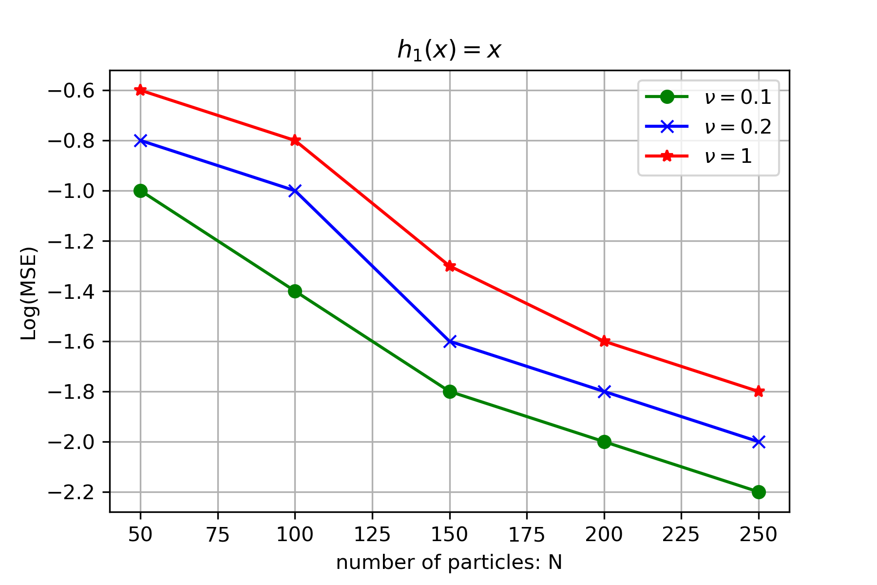
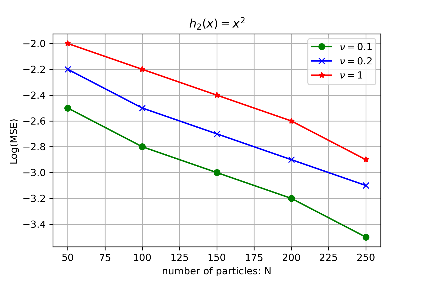
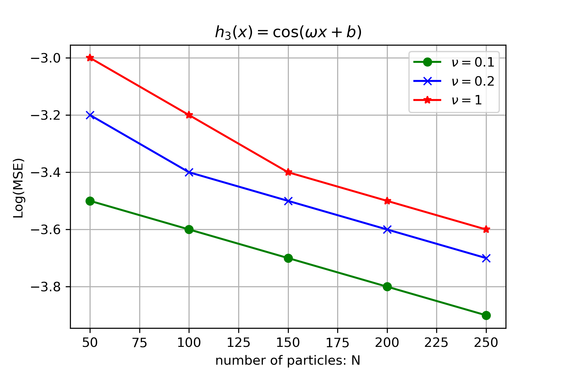
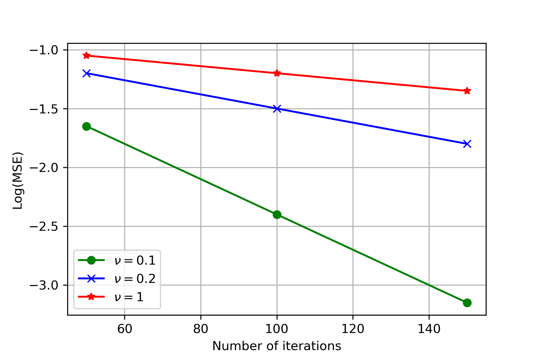
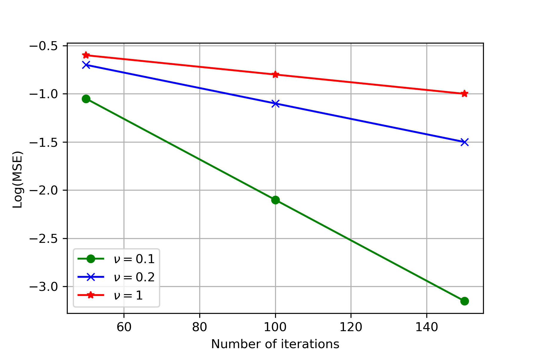
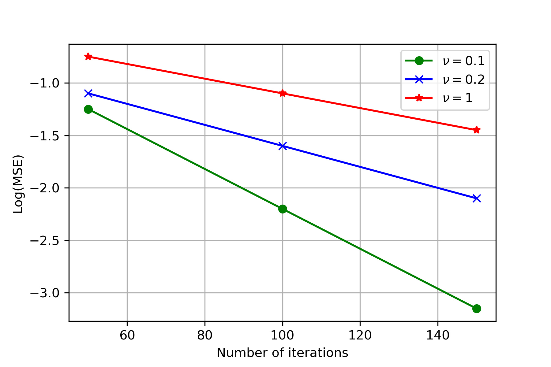
In Figure 1, we plot the mean-squared error in estimating the above expectations with the regularized and unregularized SVGD algorithm. Here, the expectation is over the intialization (and over and for ). In the top row, we report the logarithm of the mean-squared error versus the number of particles for a fixed number of iterations (set to 100). In the bottom row, we report the logarithm of the mean-squared error versus the number of iterations for a fixed number of particles (set to 200). For both algorithms, we use the Gaussian kernel , where the bandwidth parameter is set using the median heuristic [LW16]. We use the Adagrad step-size choice for both cases, following [LW16]. For the choice of the regularization parameter, we report results for various choices of . The case of corresponds exactly to the SVGD algorithm. We notice that for small values of the regularized SVGD algorithm performs better than the SVGD algorithm.
In terms of computational complexity, in comparison to the SVGD algorithm, each iteration of regularized SVGD algorithm requires inverting an matrix. It is possible to speed-up the regularized SVGD algorithm by reinterpreting the iterations as solving a system of linear equations, and using fast implementations of linear systems solvers. Other techniques for speeding-up include using Random Fourier Features and Nyström method. We leave a detailed study of speeding up the regularized SVGD algorithm as future work.
Acknowledgements
YH was supported in part by NSF TRIPODS grant CCF-1934568. KB was supported in part by NSF grant DMS-2053918. BKS was supported in part by NSF CAREER Award DMS-1945396. JL was supported in part by NSF via award DMS-2012286. Parts of this work was done when YH, KB and JL visited the Simons Institute for the Theory of Computing as a part of the “Geometric Methods in Optimization and Sampling” program during Fall 2021.
References
- [AGS05] Luigi Ambrosio, Nicola Gigli, and Giuseppe Savare. Gradient Flows: In Metric Spaces and in the Space of Probability Measures. Springer Science & Business Media, 2005.
- [AM14] Douglas Azevedo and Valdir Antonio Menegatto. Sharp estimates for eigenvalues of integral operators generated by dot product kernels on the sphere. Journal of Approximation Theory, 177:57–68, 2014.
- [BCE+22] Krishnakumar Balasubramanian, Sinho Chewi, Murat A Erdogdu, Adil Salim, and Shunshi Zhang. Towards a theory of non-log-concave sampling: First-order stationarity guarantees for Langevin Monte Carlo. In Conference on Learning Theory, pages 2896–2923. PMLR, 2022.
- [BGL14] Dominique Bakry, Ivan Gentil, and Michel Ledoux. Analysis and Geometry of Markov Diffusion Operators, volume 103. Springer, 2014.
- [BLY21] Krishnakumar Balasubramanian, Tong Li, and Ming Yuan. On the optimality of kernel-embedding based goodness-of-fit tests. Journal of Machine Learning Research, 22(1), 2021.
- [BTA11] Alain Berlinet and Christine Thomas-Agnan. Reproducing Kernel Hilbert Spaces in Probability and Statistics. Springer Science & Business Media, 2011.
- [CB16] Katy Craig and Andrea Bertozzi. A blob method for the aggregation equation. Mathematics of Computation, 85(300):1681–1717, 2016.
- [CCP19] José Antonio Carrillo, Katy Craig, and Francesco S Patacchini. A blob method for diffusion. Calculus of Variations and Partial Differential Equations, 58(2):1–53, 2019.
- [CCSW22] Yongxin Chen, Sinho Chewi, Adil Salim, and Andre Wibisono. Improved analysis for a proximal algorithm for sampling. In Po-Ling Loh and Maxim Raginsky, editors, Proceedings of Thirty Fifth Conference on Learning Theory, volume 178, pages 2984–3014, 2022.
- [CEL+21] Sinho Chewi, Murat A Erdogdu, Mufan Bill Li, Ruoqi Shen, and Matthew Zhang. Analysis of Langevin Monte Carlo from Poincaré to Log-Sobolev. arXiv preprint arXiv:2112.12662, 2021.
- [Che17] Alina Chertock. A practical guide to deterministic particle methods. In Handbook of Numerical Analysis, volume 18, pages 177–202. Elsevier, 2017.
- [CLGL+20] Sinho Chewi, Thibaut Le Gouic, Chen Lu, Tyler Maunu, and Philippe Rigollet. SVGD as a kernelized Wasserstein gradient flow of the chi-squared divergence. Advances in Neural Information Processing Systems, 33:2098–2109, 2020.
- [CSG16] Kacper Chwialkowski, Heiko Strathmann, and Arthur Gretton. A kernel test of goodness of fit. In International Conference on Machine Learning, pages 2606–2615. PMLR, 2016.
- [CX20] Lin Chen and Sheng Xu. Deep neural tangent kernel and Laplace kernel have the same RKHS. In International Conference on Learning Representations, 2020.
- [CZ07] Felipe Cucker and Ding-Xuan Zhou. Learning Theory: An Approximation Theory Viewpoint, volume 24. Cambridge University Press, 2007.
- [DM90] Pierre Degond and Francisco-José Mustieles. A deterministic approximation of diffusion equations using particles. SIAM Journal on Scientific and Statistical Computing, 11(2):293–310, 1990.
- [DNS19] Andrew Duncan, Nikolas Nüsken, and Lukasz Szpruch. On the geometry of Stein variational gradient descent. arXiv preprint arXiv:1912.00894, 2019.
- [Dob79] Roland Dobrushin. Vlasov equations. Functional Analysis and Its Applications, 13(2):115–123, 1979.
- [GDVM19] Jackson Gorham, Andrew B Duncan, Sebastian J Vollmer, and Lester Mackey. Measuring sample quality with diffusions. The Annals of Applied Probability, 29(5):2884–2928, 2019.
- [GM17] Jackson Gorham and Lester Mackey. Measuring sample quality with kernels. In International Conference on Machine Learning, pages 1292–1301. PMLR, 2017.
- [JKO98] Richard Jordan, David Kinderlehrer, and Felix Otto. The variational formulation of the Fokker–Planck equation. SIAM Journal on Mathematical Analysis, 29(1):1–17, 1998.
- [KSA+20] Anna Korba, Adil Salim, Michael Arbel, Giulia Luise, and Arthur Gretton. A non-asymptotic analysis for Stein Variational Gradient Descent. Advances in Neural Information Processing Systems, 33, 2020.
- [Liu17] Qiang Liu. Stein Variational Gradient Descent as gradient flow. Advances in Neural Information Processing Systems, 30, 2017.
- [LLJ16] Qiang Liu, Jason Lee, and Michael Jordan. A kernelized Stein discrepancy for goodness-of-fit tests. In International Conference on Machine Learning, pages 276–284. PMLR, 2016.
- [LLN19] Jianfeng Lu, Yulong Lu, and James Nolen. Scaling limit of the Stein Variational Gradient Descent: The mean field regime. SIAM Journal on Mathematical Analysis, 51(2):648–671, 2019.
- [LRLP17] Yang Liu, Prajit Ramachandran, Qiang Liu, and Jian Peng. Stein variational policy gradient. In 33rd Conference on Uncertainty in Artificial Intelligence, UAI 2017, 2017.
- [LW16] Qiang Liu and Dilin Wang. Stein Variational Gradient Descent: A general purpose Bayesian inference algorithm. Advances in Neural Information Processing Systems, 29, 2016.
- [MNY06] Ha Quang Minh, Partha Niyogi, and Yuan Yao. Mercer’s theorem, feature maps, and smoothing. In International Conference on Computational Learning Theory, pages 154–168. Springer, 2006.
- [MRZ16] Adrian Muntean, Jens Rademacher, and Antonios Zagaris. Macroscopic and Large Scale Phenomena: Coarse Graining, Mean Field Limits and Ergodicity. Springer, 2016.
- [PR16] Vern Paulsen and Mrinal Raghupathi. An Introduction to the Theory of Reproducing Kernel Hilbert Spaces, volume 152. Cambridge University Press, 2016.
- [Rav85] Pierre-Arnaud Raviart. An analysis of particle methods. In Numerical Methods in Fluid Dynamics, pages 243–324. Springer, 1985.
- [Rus90] Giovanni Russo. Deterministic diffusion of particles. Communications on Pure and Applied Mathematics, 43(6):697–733, 1990.
- [San17] Filippo Santambrogio. Euclidean, metric, and Wasserstein gradient flows: An overview. Bulletin of Mathematical Sciences, 7(1):87–154, 2017.
- [SC08] Ingo Steinwart and Andreas Christmann. Support Vector Machines. Springer Science & Business Media, 2008.
- [SGBSM20] Carl-Johann Simon-Gabriel, Alessandro Barp, Bernhard Schölkopf, and Lester Mackey. Metrizing weak convergence with maximum mean discrepancies. arXiv preprint arXiv:2006.09268, 2020.
- [SGF+10] Bharath Sriperumbudur, Arthur Gretton, Kenji Fukumizu, Bernhard Schölkopf, and Gert Lanckriet. Hilbert space embeddings and metrics on probability measures. Journal of Machine Learning Research, 11(Apr):1517–1561, 2010.
- [SH21] Meyer Scetbon and Zaid Harchaoui. A spectral analysis of dot-product kernels. In International conference on Artificial Intelligence and Statistics, pages 3394–3402. PMLR, 2021.
- [SR22] Lukang Sun and Peter Richtárik. A note on the convergence of mirrored Stein Variational Gradient Descent under -smoothness condition. arXiv preprint arXiv:2206.09709, 2022.
- [SSR22] Adil Salim, Lukang Sun, and Peter Richtarik. A convergence theory for SVGD in the population limit under Talagrand’s inequality . In International Conference on Machine Learning, pages 19139–19152. PMLR, 2022.
- [TSA20] Nicolas Garcia Trillos and Daniel Sanz-Alonso. The Bayesian update: Variational formulations and gradient flows. Bayesian Analysis, 15(1):29–56, 2020.
- [Vil21] Cédric Villani. Topics in Optimal Transportation, volume 58. American Mathematical Soc., 2021.
- [VW19] Santosh Vempala and Andre Wibisono. Rapid convergence of the Unadjusted Langevin Algorithm: Isoperimetry suffices. arXiv preprint arXiv:1903.08568, 2019.
- [Wib18] Andre Wibisono. Sampling as optimization in the space of measures: The Langevin dynamics as a composite optimization problem. In Conference on Learning Theory, pages 2093–3027. PMLR, 2018.
- [WTBL19] Dilin Wang, Ziyang Tang, Chandrajit Bajaj, and Qiang Liu. Stein Variational Gradient Descent with matrix-valued kernels. Advances in Neural Information Processing Systems, 32, 2019.
- [WZL18] Dilin Wang, Zhe Zeng, and Qiang Liu. Stein variational message passing for continuous graphical models. In International Conference on Machine Learning, pages 5219–5227. PMLR, 2018.
- [XKS22] Lantian Xu, Anna Korba, and Dejan Slepc̆ev. Accurate quantization of measures via interacting particle-based optimization. In International Conference on Machine Learning, pages 24576–24595. PMLR, 2022.