Imaging Venus’ Surface at Night in the Near-IR From Above Its Clouds:
New Analytical Theory for the Effective Spatial Resolution

Abstract

There are a handful of spectral windows in the near-IR through which we can see down to Venus’ surface on the night side of the planet. The surface of our sister planet has thus been imaged by sensors on Venus-orbiting platforms (Venus Express, Akatsuki) and during fly-by with missions to other planets (Galileo, Cassini). The most tantalizing finding, so far, is the hint of possible active volcanism. However, the thermal radiation emitted by Venus’ searing surface (c. 475^∘C) has to get through the opaque clouds between 50 and 70 km altitude, as well as the sub-cloud atmosphere. In the clouds, the light is not absorbed but scattered, many times. This results in blurring the surface imagery to the point where the smallest discernible feature is roughly 100 km in size, full-width half-max (FWHM), and this has been explained using numerical models. We describe a new analytical modeling framework for predicting the width of the atmospheric point-spread function (APSF), which is what determines the effective resolution of surface imaging from space. Our best estimates of the APSF width for the 1-to-1.2 $\mu$m spectral range are clustered around 130 km FWHM. Interestingly, this is somewhat larger than the accepted value of $\approx$100 km, which is based on visual image inspection and numerical simulations.

Keywords Venus  $\cdot$ clouds  $\cdot$ surface  $\cdot$ imaging  $\cdot$ near-IR  $\cdot$ radiative transfer

1 Introduction & Overview

Nighttime imaging by near-IR (NIR) sensors, either orbiting Venus (Venus Express, Akatsuki) or during fly-bys (Galileo, Cassini), have provided glimpses at the planet’s surface through a handful of spectral windows between CO₂ absorption bands, revealing the possible presence of active volcanism [1, 2, 3]. Surface-emitted thermal radiation must however get through optically thick light-scattering clouds between 50 and 70 km in altitude [4]. Therefore, the effective spatial resolution (ESR) of the surface imaging is poor, at $\approx$100 km, full-width half max (FWHM). This is a long-accepted fact based on visual inspection of the observations. followed by an intuitive geometrical argument [5] or detailed numerical simulations [6, 7].

In a recent study [8], we used numerical estimates of the atmospheric point-spread function (APSF) to show that sharp nighttime surface imaging is feasible from just below Venus’ clouds; see Fig. 1. Here, we present a family of analytical models for the APSF that predict it, or its at least its width, in closed form for space-based imaging. However, the best of the new models suggests somewhat larger values than currently accepted, specifically, we find values $\approx$130 km FWHM for the 1-to-1.2 $\mu$m NIR spectral subrange on which [8] focused their attention.

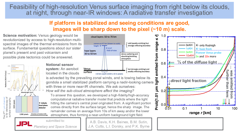
Figure 1: Graphical summary of the investigation by [8] of the feasibility of sharp nighttime NIR imaging of Venus’ thermally glowing surface from a platform located just below the clouds.

In the following Section, the clouds are modeled in a preliminary way as a thin diffusing plate at an altitude of $\approx$50 km, which is cloud-base height, and sub-cloud propagation is approximately ballistic, i.e., dominated by direct transmission. In Section 3, we adopt a more realistic representation of clouds as a multiple scattering optical medium, and apply closed-form expressions from a diffusion theoretical model developed originally for Earth observation [9]. Section 4, we summarize our findings, specifically, that the ESR in the 1-to1.2 $\mu$m wavelength range is $\approx$130 km FWHM.

2 Cloud layer as a diffusing plate at 50 km altitude

Figure 2 (top panel) is a schematic of the simplest possible conceptual model where Venus’ clouds act like a thin diffusing plate Through such a plate, one can clearly see the shape of things on the opposite side only if they are up next to it. On Venus, the objects of interest are 50 km below, so they cannot be distinguished clearly. In fact, the minimum size of any distinguishable feature is determined by a directionally averaged incoming angle, thus leading to the $\sim$100 km minimum size of a distinguishable surface feature.

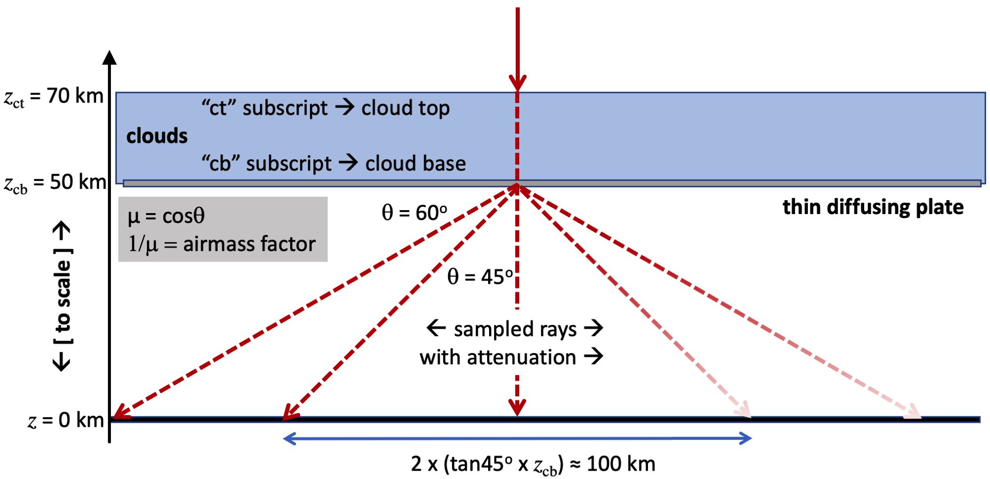
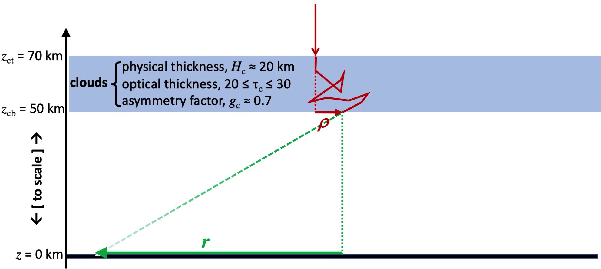
Figure 2: Schematic for the estimation of the effective resolution of surface features achievable from space. Top panel: As a first-order approximation, the clouds act as a diffusing plate; thus, the smallest resolvable feature depends only on cloud-base height (left-hand side), which is $\approx$50 km. Factoring in the extinction across the sub-cloud Rayleigh-scattering atmosphere (right-hand side), the effective resolution becomes somewhat sharper since near-nadir rays weigh in more heavily on average. Bottom panel: Conceptualization of the cloud layer as a diffusing plate is upgraded to a strongly scattering medium of finite thickness where transmitted light is dispersed away from the horizontal position of the source by a predictable RMS distance. Effective surface resolution from above the clouds is then the RMS sum of two horizontal transport mechanisms: multiple scattering inside the cloud, and attenuated ballistic propagation below the cloud. See text for further details.

Table 1: From left to right: Venus’ sub-cloud atmosphere’s optical thickness for Rayleigh scattering at three NIR wavelengths of interest, being CO₂ absorption windows. Total optical thickness, including an empirical band-wide estimate of gaseous absorption impacts. Predictions for the RMS diameter $2r_{\text{RMS}}$ (and FWHM) of the APSF for our three models for the impact of clouds: (1) clouds as a thin diffusing plate; (2) asymptotic diffusion theory; (3) with pre-asymptotic corrections. In all cases, the sub-cloud propagation is modeled as ballistic, with the appropriate attenuation; see Eq. (2). For Models 2 and 3, a Gaussian shape is assumed for the APSF, hence FWHM = 1.18$\,\times\,2r_{\text{RMS}}$. For Model 1, the APSF’s shape is not Gaussian, and the expression in (3) is used for the FWHM.

$\lambda$ [$\mu$m]	$\tau_{\rm R}$	$\tau_{\rm t}$	Model 1 [km]	Model 2 [km]	Model 3 [km]
1.01	1.43	1.43	107 (114)	111 (131)	113 (133)
1.10	1.09	1.64	100 (105)	106 (125)	108 (127)
1.18	0.77	1.54	103 (108)	108 (127)	110 (130)

A closer look at the right-hand side of the top panel in Fig. 2 reminds us that the sub-cloud space is not transparent. Directly-transmitted incoming light is extinguished across the medium by an amount that depends only on its optical thickness and the incoming zenith angle $\theta$. Ruling out the possibility of haze, for simplicity, optical thickness is the Rayleigh scattering value $\tau_{\rm R}$ listed in Table 1. Probability of direct transmission is then $\exp(-\tau_{\rm R}/\mu)$ where we recognize the airmass factor $1/\mu$, with $\mu=\cos\theta$.

Now we can estimate the mean and root-mean square (RMS) value of the horizontal transport distance across the medium, namely, $r=z_{\text{cb}}\tan\theta$ where $z_{\text{cb}}$ is identified as the cloud base height in Fig. 2, which are drawn to scale. Specifically, we have

$$\langle r^{q}\rangle=z_{\text{cb}}^{q}\,\langle\tan^{q}\theta\rangle=z_{\text{cb}}^{q}\int\limits_{0}^{1}\left(\frac{1}{\mu^{2}}-1\right)^{q/2}{\rm e}^{-\tau_{\rm R}/\mu}{\rm d}\mu\left/\left[{\rm e}^{-\tau_{\rm R}}-\tau_{\rm R}\Gamma(0,\tau_{\rm R})\right]\right.\!,$$ (1)

where $q=1,2$ yield respectively the 1${}^{\text{st}}$ and 2${}^{\text{nd}}$ moments of $r$, the modulus of the random horizontal vector $\mathbf{r}=(r\cos\phi,r\sin\phi)$ with $\phi$ being the azimuthal angle. In short, (1) yields the mean $\langle r\rangle$ of $r$ and the variance $\langle\mathbf{r}^{2}\rangle$ of $\mathbf{r}$ since $\langle\mathbf{r}\rangle$ vanishes by rotational symmetry. From the latter quantity, we can obtain $r_{\text{RMS}}=\sqrt{\langle\mathbf{r}^{2}\rangle}$. The normalization factor in the denominator of (1) is the result of the integral in the numerator when $q=0$; therein, $\Gamma(a,x)$ is the incomplete Euler Gamma function.

When $q=1$, the integration is performed numerically, but when $q=2$, we have a closed-form expression:

$$\langle\mathbf{r}^{2}\rangle=z_{\text{cb}}^{2}\,\langle\tan^{2}\theta\rangle=z_{\text{cb}}^{2}\left[{\rm e}^{-\tau_{\rm R}}\left(1/\tau_{\rm R}-1\right)+\tau_{\rm R}\Gamma(0,\tau_{\rm R})\right]\left/\left[{\rm e}^{-\tau_{\rm R}}-\tau_{\rm R}\Gamma(0,\tau_{\rm R})\right]\right.\!.$$ (2)

For the three finite values of $\tau_{\rm R}$ in Table 1, we find $2r_{\text{RMS}}=2\sqrt{\langle\mathbf{r}^{2}\rangle}$ = 107, 120 and 140 [km], respectively for $\lambda$ = 1.01, 1.10 and 1.18 [$\mu$m] when $z_{\text{cb}}$ = 50 km. For $q$ = 1, numerical quadrature of the integral in (1) yields respectively $2\langle r\rangle$ = 88, 98 and 112 [km].

Another popular measure of spatial resolution using the APSF is the full-width half-max (FWHM) distance. Denoting the extinction coefficient as $\sigma_{\rm R}=\tau_{\rm R}/z_{\text{cb}}$, we identify the azimuthally-invariant APSF($r$) in (1), as $\propto\exp\left(-\sigma_{\rm R}\sqrt{z_{\text{cb}}^{2}+r^{2}}\right)$, that is, $\exp\left(-\tau_{\rm R}/\mu_{r}\right)$. In this case,

$$\text{FWHM}=2z_{\text{cb}}\sqrt{(2\ln 2)\tau_{\rm R}+(\ln 2)^{2}}/\tau_{\rm R},$$ (3)

and the three values of $\tau_{\rm R}$ in Table 1 yield 114, 134 and 167 [km].

We note that, in the limit $\tau_{\rm R}\to 0$ that is implicit in the left-hand side of Fig. 2 (upper panel), both mean and variance in (1) diverge due to the grazing view angles, $\theta\approx\pi/2$. The FWHM parameter in (3) also becomes infinite for the same reason. Therefore, in the absence of sub-cloud extinction, we need to estimate the effective surface resolution by choosing a typical value of $\theta$ and injecting it into $r=z_{\text{cb}}\tan\theta$. We illustrate the natural choice of 60${}^{\circ}=\cos^{-1}\langle\mu\rangle$, yielding 173 km, which seems too big. Following [5], we can rationalize the choice of 45^∘, leading to the more reasonable estimate of $2z_{\text{cb}}$ = 100 km resolution side-to-side.

So far, we have only accounted for extinction from Rayleigh scattering, which is a reasonable approximation for the shortest NIR wavelength under consideration (i.e., $\lambda\approx$ 1 $\mu$m). For the longest ($\lambda\approx$ 1.2 $\mu$m), we cannot neglect absorption by gases (both CO₂ and H₂O contribute). [8] did that (in their Appendix A) using an effective SSA${}_{\text{g}}<1$ in the atmospheric column, which was empirically estimated to be $\approx$1/2 for $\lambda$ = 1.18 $\mu$m and, for $\lambda$ = 1.10 $\mu$m, it was $\approx$2/3. Now, using total optical thickness $\tau_{\rm t}=\tau_{\rm R}/$SSA${}_{\text{g}}$ in (2), we update 2$r_{\text{RMS}}$ in (2) to 100 and 103 km, respectively for $\lambda$ = 1.10 and 1.18 $\mu$m, while the FWHM in (3) are reduced to 105 and 108 km.

These analytical estimates of the FHWM of the atmospheric spatial filter based on APSF moments are slightly larger than the $\sim$100 km value estimated numerically by [6] and [7], who account for multiple scattering in the cloud layer. They follow, however, from a simple APSF model based only on attenuated ballistic propagation of the NIR light emanating from the surface across the sub-cloud optical medium.

3 Cloud layer as a multiple-scattering optical medium

We now turn to the lower panel of Fig. 2 where we again upgrade our APSF model by relaxing the assumption of a diffusing plate with virtually no thickness to mimic the blurring effect of the cloud layer. Instead, we now have two layers with finite optical and physical thicknesses that each disperse according to their individual APSFs the “reciprocal” (time-reversed) light that starts at a single point source at the upper boundary of the top layer. Conversely, light emanating from a whole region at the lower boundary of the bottom layer propagates to the interface between the two layers, and a single pixel from the space-based sensor receives light from a whole region of that interface. What is the size of the primary source region at the surface? Conversely, what is the size of the spot of time-reversed light at the surface? Either way, that will be the effective spatial resolution of the space-based sensor for features on the planetary surface.

In this problem, the most useful measure of APSF width is the RMS radius that we continue to denote $r_{\text{RMS}}=\sqrt{\langle\mathbf{r}^{2}\rangle}$ for the sub-cloud layer, and introduce $\rho_{\text{RMS}}=\sqrt{\langle\boldsymbol{\rho}^{2}\rangle}$ for the cloud layer. These RMS radii will both scale as the physical thickness of the layer, 50 km for the sub-cloud layer (denoted $z_{\text{cb}}$ in Fig. 2) and $\approx$20 km for the cloudy layer (denoted $H_{\rm c}$ in the lower panel of Fig. 2). Our best estimates for $r_{\text{RMS}}$ using the attenuated ballistic propagation model that we have used so far for the sub-cloud APSF are: $r_{\text{RMS}}$ = 107, 100 and 103 [km] for $\lambda$ = 1.01, 1.10 and 1.18 [$\mu$m], respectively.

We are now dealing with the sum of two random horizontal vectors $\mathbf{r}$ and $\boldsymbol{\rho}$, both with vanishing means. We can therefore invoke the additivity property of the so-called “cumulant” moments and, in this case, only the first two are of interest. The means yield $\langle\boldsymbol{\rho}+\mathbf{r}\rangle=\langle\boldsymbol{\rho}\rangle+\langle\mathbf{r}\rangle=\mathbf{0}$. The variances yield

$$\langle(\boldsymbol{\rho}+\mathbf{r})^{2}\rangle=\langle\boldsymbol{\rho}^{2}\rangle+\langle\mathbf{r}^{2}\rangle,$$ (4)

where $\langle\mathbf{r}^{2}\rangle$ was estimated in Section 2. For the new quantity, $\rho_{\text{RMS}}$, we can use outcomes from the theoretical investigation by [9] of the Green functions of optically thick clouds for transmitted light at non-absorbing wavelengths. In sharp contrast with our present ballistic propagation model for the sub-cloud medium, the authors used the diffusion approximation where light propagates across the medium in the manner of a random walking particle, specifically, many small steps in random directions. In terrestrial as well as Venusian clouds, the particulates are commensurate or larger than the NIR wavelengths of interest here [10, 11] They are therefore have quite strongly forward-scattering phase functions, with asymmetry factors $g_{\rm c}\approx 0.7$. Specifically, [9] show that $\rho_{\text{RMS}}\approx\sqrt{2/3}\,H_{\rm c}$, irrespective of the scattering phase function in the limit of large “scaled” optical thickness, i.e., $(1-g_{\rm c})\tau_{\rm c}\gg 1$. They also computed the correction term for finite values of $(1-g_{\rm c})\tau_{\rm c}$, namely, $\sqrt{1+(3+4X)/2X(1+X)}$ where $X=(3/4)(1-g_{\rm c})\tau_{\rm c}$.

Combining our predictions for the sub-cloud layer and those of [9] for the cloudy layer according to (4), we find that the overall APSF has an 2$\times$RMS size of $2\sqrt{\langle\boldsymbol{\rho}^{2}\rangle+\langle\mathbf{r}^{2}\rangle}$ = 111, 106 and 108 [km], respectively, for $\lambda$ = 1.01, 1.10 and 1.18 [$\mu$m]. Neglecting in-cloud absorption by gases is justified at the longer wavelengths (where it matters in the sub-cloud layer) because molecular densities have decreased to a very small fraction of their near-surface values. Davis and Marshak’s small correction for the range of values assumed for $\tau_{\rm c}$ in the lower panel of Fig. 2 is an increase of $\approx$16% in $\rho_{\text{RMS}}$. This modest boost in $\rho_{\text{RMS}}$ leads to 113, 108 and 110 [km], respectively, for (2 RMS) = $2\sqrt{\langle\boldsymbol{\rho}^{2}\rangle+\langle\mathbf{r}^{2}\rangle}$, which is always dominated by the latter (sub-cloud) contribution.

To convert our estimates of the RMS radius into the more widely used FWHM in spatial filtering, we assume a Gaussian shape for the APSF. This leads to FWHM = $\sqrt{2\ln\!2}\times$(2 RMS) $\approx 1.1774\times$(2 RMS). The FWHM values associated with our above best estimates of (2 RMS) are 133, 127, and 130 [km], respectively, for $\lambda$ = 1.01, 1.10 and 1.18 [$\mu$m].

4 Conclusion

We have used the atmospheric point-spread function (APSF) concept to predict from first principles the effective resolution of near-IR imagery of Venus surface features captured by space-based sensors, either orbiting or during a flyby. Physically, the APSF quantities the transport of surface-emitted thermal radiation in the horizontal plane (i.e., across the imaging sensors’ pixels) between the actual source and the surface point at which a given pixel is pointing. Our APSF model is analytical, combining the two extreme propagation modes in radiative transfer: ballistic (below clouds) and diffusive (in clouds). The clouds are first represented by a thin diffusing plate that does not add any lateral transport of the NIR light. Next, they are given a finite thickness and opacity, thus enabling horizontal radiation transport inside the clouds, as modeled by [9], which is combined with the (dominant) contribution of the sub-cloud angular spread. Our final estimates across the 1-to-1.2 $\mu$m wavelength range are narrowly clustered around $\approx$130 km full-width half-max (FWHM). They thus verify analytically the accepted value of $\approx$100 km FWHM, but suggest a somewhat larger number.

©2022. California Institute of Technology. Government sponsorship acknowledged.

References

- [1] Suzanne E Smrekar, Ellen R Stofan, Nils Mueller, Allan Treiman, Linda Elkins-Tanton, Joern Helbert, Giuseppe Piccioni, and Pierre Drossart. Recent hotspot volcanism on Venus from VIRTIS emissivity data. Science, 328(5978):605–608, 2010.
- [2] NT Mueller, S Smrekar, J Helbert, E Stofan, G Piccioni, and P Drossart. Search for active lava flows with VIRTIS on Venus Express. Journal of Geophysical Research: Planets, 122(5):1021–1045, 2017.
- [3] P. K. Byrne and S. Krishnamoorthy. Estimates on the frequency of volcanic eruptions on venus. Journal of Geophysical Research: Planets, page e2021JE007040, 2020.
- [4] Dmitrij V Titov, Nikolay I Ignatiev, Kevin McGouldrick, Valérie Wilquet, and Colin F Wilson. Clouds and hazes of Venus. Space Science Reviews, 214(8):1–61, 2018.
- [5] V. I. Moroz. Estimates of visibility of the surface of Venus from descent probes and balloons. Planetary and Space Science, 50(3):287–297, March 2002.
- [6] George L Hashimoto and Takeshi Imamura. Elucidating the rate of volcanism on Venus: Detection of lava eruptions using near-infrared observations. Icarus, 154(2):239–243, 2001.
- [7] Alexander T Basilevsky, Eugene V Shalygin, Dmitri V Titov, Wojciech J Markiewicz, Frank Scholten, Th Roatsch, Michail A Kreslavsky, Ljuba V Moroz, Nikolay I Ignatiev, B Fiethe, B Osterloh, and H Michalik. Geologic interpretation of the near-infrared images of the surface taken by the Venus Monitoring Camera, Venus Express. Icarus, 217(2):434–450, 2012.
- [8] A. B. Davis, K. H. Baines, B. M. Sutin, J. A. Cutts, L. I. Dorsky, and P. K. Byrne. Feasibility of high-spatial-resolution nighttime near-IR imaging of Venus’ surface from a platform just below the clouds: A radiative transfer study accounting for the potential of haze. Planetary and Space Science, 2022. (submitted, revised).
- [9] Anthony B Davis and Alexander Marshak. Space-time characteristics of light transmitted through dense clouds: A Green’s function analysis. Journal of the Atmospheric Sciences, 59(18):2713–2727, 2002.
- [10] R G Knollenberg and D M Hunten. The microphysics of the clouds of Venus: Results of the Pioneer Venus particle size spectrometer experiment. Journal of Geophysical Research: Space Physics, 85(A13):8039–8058, 1980.
- [11] B Ragent, LW Esposito, MG Tomasko, M Ya Marov, VP Shari, and VN Lebedev. Particulate matter in the Venus atmosphere. Advances in Space Research, 5(11):85–115, 1985.