How the form of weighted networks impacts quantum reservoir computation

Abstract

Quantum extreme reservoir computation (QERC) is a versatile quantum neural network model that combines the concepts of extreme machine learning with quantum reservoir computation. Key to QERC is the generation of a complex quantum reservoir (feature space) that does not need to be optimized for different problem instances. Originally, a periodically-driven system Hamiltonian dynamics was employed as the quantum feature map. In this work we capture how the quantum feature map is generated as the number of time-steps of the dynamics increases by a method to characterize unitary matrices in the form of weighted networks. Furthermore, to identify the key properties of the feature map that has sufficiently grown, we evaluate it with various weighted network models that could be used for the quantum reservoir in image classification situations. At last, we show how a simple Hamiltonian model based on a disordered discrete time crystal with its simple implementation route provides nearly-optimal performance while removing the necessity of programming of the quantum processor gate by gate.

I Introduction

In recent years we have seen the steady growth of the number of qubits available on a variety of quantum processors [1, 2, 3, 4]. This has led to the new phase of quantum computer development, often called the “NISQ” era. Here NISQ stands for noisy intermediate-scale quantum, which indicates that the quantum processor is too small to implement logical quantum operations and hence is inherently noisy. The number of qubits in these quantum processors (well in excess of 50 [3, 5, 6]) has already reached the point where the quantum computational tasks they can perform are intractable in a conventional computer, however noise prevents us to extract the quantum advantage such quantum computer promise. Hence, for the NISQ era to mark its significance in computer history, quantum advantages for real applications have to be demonstrated.

Many of the current NISQ processors are designed to operate via quantum gates [1, 7, 8, 9]. To run a quantum algorithm, we need to obtain a quantum gate circuit from the quantum algorithm, and then to decompose each quantum gate into ones implementable on the quantum processor at hand. The noise in these quantum processors necessitates the optimization of quantum gate circuits to minimize their effect. As long as the physical qubits are directly used for computation, quantum algorithms also need to be relatively short and resilient to noise. Variational quantum algorithms (VQAs) have attracted a lot of attention from this viewpoint and have been intensively investigated [10, 11, 12]. However there have been several issues with them with the most significant obstacle being the difficulty in the optimization of the variational models [13, 14]. Variational quantum algorithms are a type of model of quantum neural networks (QNNs). It is well known that there are other models for using QNNs. One such example is quantum reservoir computation [15, 16, 17, 18] which should be expected to be more implementation friendly. Similarly to the chaotic dynamics used in the (classical) reservoir computation [19, 20], the quantum reservoir is to generate complex dynamics in the quantum system. Realizing such dynamics using a quantum gate circuit approach is however not that simple [21, 22, 23, 24, 1]. We do not require precise programming to generate a sufficient complexity in quantum reservoir to realize our quantum algorithm[16, 18]. Instead an effective quantum reservoir can potentially be generated by a simpler quantum system giving us a better way to utilize the computational power of QNNs.

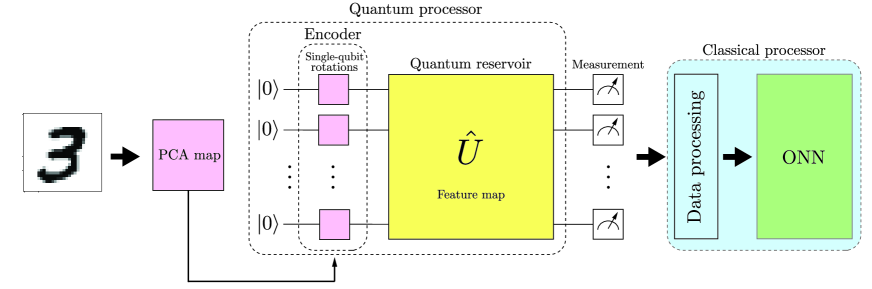
Figure 1: Schematic architecture of the quantum extreme reservoir computation (QERC) processor. It begins with an image of size $28\times 28$ pixels is processed through principal component analysis and compressed to $2L$ components (where $L$ is the number of qubits). Using these $2L$ components, an initial state corresponding to the image is created by single-qubit rotations. The quantum reservoir then lets the initial state evolve. By projective measurements in the computational basis, the final state is converted to classical information. The amplitude distribution of this classical information, it is fed into the one-layer neural network (ONN).

Recently quantum extreme reservoir computation (QERC) was proposed [25] as a more advanced yet simplier QNN model based on quantum reservoir computation and extreme machine learning [26]. This model uses a quantum reservoir to generate a quantum neural network which is then for extreme machine learning. So far, this model has numerically shown to achieve the highest accuracy to classify hand written digits using MNIST data set with the smallest number of qubits [27]. An interesting feature of this approach is that it utilizes a discrete time crystal (DTC) as the feature map, which is much simpler to implement than the quantum gate circuit needed to generate a random unitary matrix. This suggests that if we could understand the mechanism associated with using the complexity of the quantum dynamics for generating an effective feature space, it would become possible to design quantum feature maps more efficiently.

Now let us outline the focus and structure of this paper. We will use the QERC proposed in [25] as a tool to investigate the role of the feature map in quantum neural networks. This model provides a convenient platform to do so as the quantum contribution fully relies on quantum reservoir. We start in Section II with a description of the QERC model while we investigate the feature map properties in Section III. Then in Section IV we discuss the relation between these properties and the performance of the QERC in Section IV. We summarize in Section V our results.

II the QERC model and it’s characterization

Let us begin with a brief description of QERC. As shown in Fig. 1, QERC can be described in terms of three key components: the encoder, the quantum reservoir and the classical processor:

Encoder

Here the data to be classified is preprocessed (if necessary) and encoded into the initial state of the quantum reservoir. In more detail as shown in Fig. 1 a Principal Component Analysis (PCA) map is used for the preprocessing of the classical data. Then an appropriate encoding strategy needs to be chosen for a problem at hand. For a quantum reservoir of $L$ qubits, the $2L$ most significant parameters from the PCA map will be encoded by single-qubit rotations.

Quantum reservoir

In this step the quantum reservoir provides the feature space for QERC. The quantum dynamics of the quantum reservoir determines the feature-map properties for the quantum computation, which is given by the unitary operator $\hat{U}$.

Classical processor

In this final step, the state given by the unitary operator $\hat{U}$ acting on the initial state is measured projectively in the computational basis. The process will be repeated to obtain the amplitude distribution of the state generated by the unitary operator. This amplitude distribution is then processed through a one-layer neural network (ONN).

We immediately notice that this is a hybrid quantum-classical algorithm. In QERC the feature space is provided by the quantum reservoir, whereas the optimization is carried out on the classical processor (ONN). Typically the quantum reservoir does not need to be optimized for different problem instances [25, 15, 18].

Now our interest in this paper is the properties we require for the quantum reservoir and their influence on the performance of QERC. In particular we want to show that how we set the quantum reservoir is important. In this work we first employ the DTC model used in [25] as our choice of quantum reservoir. The DTC model has a parameter which controls the complexity of the dynamics; namely starting with the perfect discrete time crystal when the rotation parameter error $\epsilon=0$, the dynamics gradually deviates from a DTC acquiring its complexity as $\epsilon$ increases. This parameter $\epsilon$ represents imperfection in the single qubit rotation in the DTC Hamiltonian, which is given by

$$\hat{H}(t)=\begin{cases}\hat{H}_{1}=\hbar g(1-\epsilon)\sum_{l}\hat{\sigma}^{x}_{l}&t\in[0,T/2)\\ \hat{H}_{2}=\hbar\sum_{lm}J_{lm}\hat{\sigma}^{z}_{l}\hat{\sigma}^{z}_{m}+\hbar\sum_{l}D_{l}\hat{\sigma}^{z}_{l}&t\in[T/2,T)\end{cases}$$ (1)

where $\hat{\sigma}^{a}_{l}\ (a=x,y,z)$ represent the Pauli operators on the $l$-th qubit. Next $T$ is the cycle of the driving, while the DTC cycle is $2T$. Further $g$ is the rotation strength and in this case we set $gT=\pi$. Now $J_{lm}=J_{0}/\lvert l-m\rvert^{\alpha}$ is the coupling strength between the qubits $l$ and $m$ with a power-law decay that scales with a constant $\alpha$. Finally $D_{l}$ is a disordered external field for each qubit $l$. Unless explicitly stated, all the $D_{l}T$ are set to zero in this work.

The time-periodic system is conveniently characterized by the Floquet operator $\hat{\mathcal{F}}=\exp\left[-i\hat{H}_{2}T/2\hbar\right]\exp\left[-i\hat{H}_{1}T/2\hbar\right]$ where the stroboscopic time-evolution can be obtained by the unitary operator $\hat{U}(nT,0)=\hat{\mathcal{F}}^{n}$ for $n\in\mathbb{N}$. Hence, we use the unitary operator $\hat{U}(nT,0)$ for different values of $n$ to characterize the quantum reservoir.

II.1 Characterization of the unitary matrices

The next step is the characterization of the unitary operator $\hat{U}(nT,0)$. This unitary operator acts as a map between the input and the output states given by the feature map used for the quantum computation. Such a map can be considered as a weighted network [28, 29], however as the unitary operators are defined on the complex field, the translation to a weighted network is not trivial. Here we apply a generator decomposition of a unitary matrix $U\in$ U($N$), where $N$ is the dimension of the unitary matrix, in order to represent the unitary operator as a weighted network. The generators of U($N$) are the Hermitian matrices forming the Lie algebra [30].

Now a unitary matrix $U\in$ U($N$) can be written in the form $U=e^{-iG}$ where $G$ is a Hermitian matrix. This Hermitian matrix can be represented with real coefficients $a_{lm},b_{lm}$, and $c_{k}$ by the decomposition of $G$ with respect to the generators $\lambda$ as

$$G=\sum_{l<m}(a_{lm}\lambda^{x}_{lm}+b_{lm}\lambda^{y}_{lm})+\sum_{k}c_{k}\lambda^{z}_{k},$$ (2)

where those $\lambda$ generators are given by [30]

$$(\lambda^{\nu}_{lm})_{ij} = \delta_{li}\delta_{mj}\sigma^{\nu}_{12}+\delta_{lj}\delta_{mi}\sigma^{\nu}_{21}\ \ \ (\nu=x,y),$$ (3)

$$\lambda^{z}_{k} = \sqrt{\frac{2}{k(k+1)}}~{}\text{diag}(\underbrace{1,\cdots,1}_{k~{}\text{times}},-k,0,\cdots,0)$$ (4)

$$\lambda^{z}_{N} = I.$$ (5)

Here $\delta_{ij}$ represents the Kronecker delta, $\sigma^{\nu}_{ij}$ ($\nu=x,y$) is the ($i,j$)-component of the Pauli matrices and $I$ the identity matrix. Next $G$ as a weight matrix has three components $x,y,$ and $z$ with $\{a_{lm}\},\{b_{lm}\}$ and $\{c_{k}\}$ being the $x,y$ and $z$ contributions of the weight matrix, respectively. To convert the weight matrix to its weight distribution, we count how many coefficients are in a certain value window $(s,s+ds]$ for $s,ds\in\mathbb{R}$. This gives us a histogram to show how likely the coefficients are to take a certain value. In numerical calculations, we take 100 segments for each coefficient set to determine the value of $ds$.

Next the Hermitian matrix $G$ obtained from the unitary matrix $U$ is not necessarily unique. To uniquely determine $G$ for a given unitary matrix, we employ the principal logarithm of a matrix [31] in our numerical analysis. If $A$ is a complex-valued matrix of dimension $N$ with no eigenvalues on the negative real line $\mathbb{R}^{-}$, then there is a unique logarithm $X$ of a matrix $A$ such that all of its eigenvalues lie in the strip $\{z:-\pi<\text{Im}(z)<\pi\}$. Here $X$ is called as the principal logarithm of $A$ and denoted by $X=\log(A)$. For the DTC model we compute the Hermitian matrix for period $n$, $G(n)=i\log(\hat{U}(nT,0))$ noting that $G(n)$ is not simply equal to $n\times G(1)$.

II.2 Simulation setup for the QERC

We begin our considerations here by first directly evaluating the properties of the feature map generated by our DTC dynamics using the method outlined above. Setting a computational task is not essential to do the analysis, however it is extremely useful when later we compare these properties to the performance of the QERC. It is convenient to set a computational task to evaluate both at the same time and on similar footing. In this paper we use the well known MNIST dataset [32] where each image has $784\ (=28\times 28)$ pixels. We employ PCA to reduce each image data to the $2L$ components, which can be then encoded in the initial state of the quantum reservoir of $L$ qubits by single-qubit rotations. Finally to optimize the parameters of the ONN, we employ the stochastic gradient descent method used in [25]. Throughout this work our parameters are set as $L=10$, $J_{0}T=0.12$ with $\alpha=1.51$, These are compatible with the current ion trap experiments[33]. We also set $\epsilon=0.03$ as the highest accuracy rate has been reported for the QERC with this parameter value [25].

III Quantum reservoir weight distribution

It is important to emphasize that unless perfectly periodical, the quantum dynamics of the DTC model deviates from its initial state in time as it evolves. This allows for the growth of the complexity in the system. To observe such complexity growth in the unitary dynamics, we evaluate the weight distribution of $G(n)$ for various time periods: $n=2,10,50$ and 100. From Eq.2, we can determine the real coefficients $a_{lm},b_{lm}$ and $c_{k}$ characterizing $G(n)$ for each $n$. The Hermitian weight matrix $G(n)$ is equivalent to the $n$-period effective Hamiltonian up to the constant factor $\hbar/nT$. Thus, the diagonal (corresponding to $\{c_{k}\}$) and off-diagonal (corresponding to $\{a_{lm}\},\{b_{lm}\}$) entries of $G(n)$ are associated with the energies of the basis states and the transition energies between the basis states, respectively.

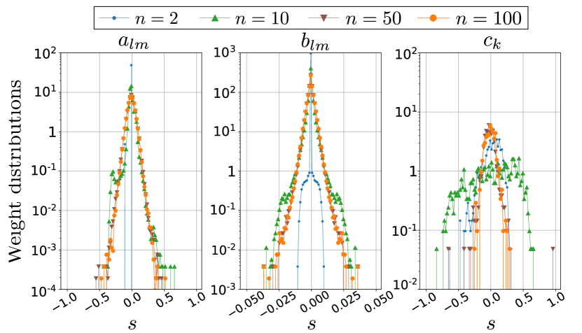
Figure 2: Convergence of the weight distribution in the DTC model. From the left to right panels, the weight distribution functions for $a_{lm},b_{lm}$ and $c_{k}$ are depicted where the colors corresponds to different periods. the blue (dot), green (upward triangle), brown (downward triangle), and orange (filled circle) curves are for $n=2,10,50$ and 100 respectively.

In Fig  2 we plot the weight distribution for the $x$ ($a_{lm}$), $y$ ($b_{lm}$) and $z$ ($c_{k}$) components of $G(n)$ respectively. Each color (symbol) represents a different period of the time evolution. For $n=2$ (blue line), we observe very sharp peaks at $s=0$ for the $x$ and $y$ components. As these components correspond to the off-diagonal entries of the Hermitian matrix $G(n)$, the sharp peaks around $s=0$ means very few transitions between the basis states for this time period. However for large periods, $n=50$ (brown curve), 100 (orange curve), the weight distributions for all the components converge to a similar shape that is approximately quadratic in the log-scaled plots (gaussian in linear plot). The weight distributions for $x$ and $y$ components has a long tail with a few nonzero elements for large $a_{lm},b_{lm}$. These nonzero elements are expected to have a significant impact in the dynamics as they indicate strong transitions between the basis states characterizing $G(n)$. In the middle of these two time regions, at $n=10$ (green curve) the $x$ and $y$ components have already converged to the typical distribution, however the $z$ component has broadened the most. This suggests that there is a tradeoff in this time regime; the stationary elements of the $z$ component significantly suppress the effect of the $x$ and $y$ components. This trade-off captures the dynamics of the DTC melting slowly in time in this ($\epsilon=0.03$) parameter regime.

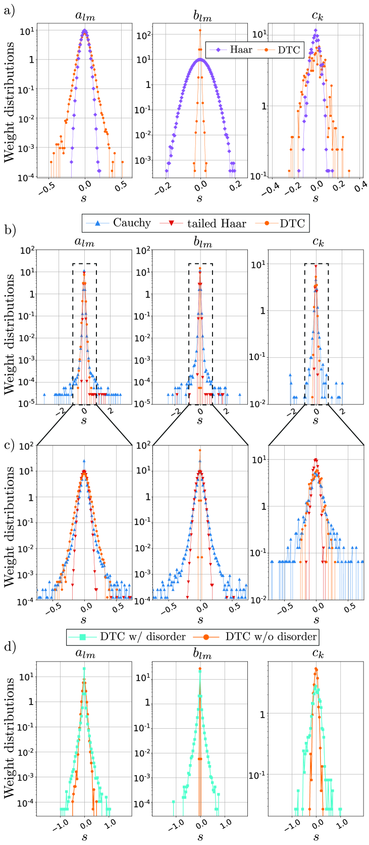
Figure 3: Comparison of the Haar-random and DTC models in a) and the Cauchy-random and DTC models in b) for $n=100$. In each case from the left to right panels, the distributions of $a_{lm},b_{lm}$ and $c_{k}$ are depicted respectively. In c), the components of Cauchy-random and DTC models are shown for the range $[-0.75,0.75]$. Finally in d) a comparison is shown between the DTC model with and without disorder for $n=100$.

III.1 Comparing the weight distribution

To capture the characteristics of the weight distribution for the DTC model, we first introduce the Haar measure sampling of unitary operators [34, 24, 35]. The Haar measure sampling can be considered to exhibit a typical complexity which a quantum computer may provide, and its gate implementation is usually given through unitary t-design [21, 22]. Hence the similarity and disparity in the weight functions for these cases would give us valuable insights to understand the DTC dynamics and its role in QERC. In our analysis, to obtain a typical distribution given by the Haar measure sampling, the $N\times N$ unitary matrix $U_{\text{H}}$ is created using the QR decomposition [36] where $N=2^{L}=2^{10}=1024$. We compare this unitary map, which we refer to as the Haar-random model to the converged weight distribution of the DTC model.

Now as shown in Fig. 3a), the typical weight distributions are approximately Gaussian for all components $a_{lm},b_{lm}$ and $c_{k}$. Here we use only one sample from the Haar-random model, since one sample and not the average of many samples will be used within the QERC. Further we do not lose generality as discussed in Appendix. A. The weight distribution functions for unitary matrices $U_{\text{H}}$ are quadratic in the log-scaled plot for all components. Their standard deviation is $\sigma\approx 0.04$ by the Gaussian fitting.

We can now compare the DTC model to the Haar-random model where we characterize the weight distributions of the DTC model with two properties, broadness and tail. Although the DTC’s $y$-component has a narrower distribution compared to the Haar-random model the broadness of the distribution for the $x$- and $z$- components are quite similar. However, only the DTC model has a tail in the weight distribution of the $x$ component.

Next to explore the difference associated with the tail we found in the DTC models distribution, we employ the Cauchy distribution. The reason for this is as follows. In classical reservoir computation, the Cauchy distribution was used to obtain the edge of chaos where the reservoir computation should be optimal [37]. Hence it is interesting to see the properties of the feature map generated by the Cauchy distribution. The Cauchy distribution is given by

$$\text{Cauchy}(x;\gamma)=\left(\frac{1}{\pi\gamma}\right)\frac{1}{1+(x/\gamma)^{2}},$$ (6)

where $\gamma$ is the scale parameter. Since the Cauchy distribution has a power-law tail, one would expect that the weight distribution exhibits a long tail. The unitary matrix $U_{\text{C}}$ for this Cauchy-random model is defined as follows. First we generate a complex-valued $N\times N$ matrix $A$ whose real and imaginary parts in each entry are drawn from the Cauchy distribution (6). Then we take a Hermitian operator $B=(A+A^{\dagger})/2$. Finally, we define the unitary matrix $U_{\text{C}}$ as $U_{\text{C}}=e^{-iB}$. Further we set $\gamma=0.04$ in Eq. 6 for consistency with the corresponding parameter of the Haar-random model ($\sigma\approx 0.04$) and the size $N$ is set as $N=2^{L}=1024$.

Applying the decomposition (2) to $G_{\text{C}}=i\log(U_{\text{C}})$, we obtain each weight distribution for the three components $a_{lm},b_{lm}$ and $c_{k}$., which are depicted in Fig. 3b). The weight distributions for the Cauchy-random model definitely have a tail, much longer than that in the DTC model, for all the components $x$, $y$, and $z$. This reflects the nature of the Cauchy distribution (6), and we will come back to this point later.

IV Relation between the QERC performance and the weight distribution

As we have characterized the three models through the weight distribution, let us now turn our attention to the performance of the QERC employing these three different models as its feature space. In the previous work [25] it was shown that the accuracy of the QERC increases with the number of the time periods of the DTC model saturating near $n=50$. The behaviour of this accuracy rate can be predicted from the time evolution of the weighted distributions seen in Fig. 2, as the unitary map of the DTC model acquires the typical complexity around $n=50$. To illustrate this further Fig. 4 summarizes the comparison between the accuracy rate and the weigh distribution. Here we plot the accuracy rates for training (blue dot) and testing (orange downward triangle) against the time period $n$ in the DTC model and insert the weight distributions for $n=2,10,50,100$.

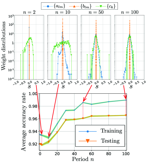
Figure 4: Average accuracy rates for training and testing with the associated standard deviation against the period in the DTC model. The blue (dot) and orange (downward triangle) curves correspond to training and testing, respectively. At each datapoint, the average and the standard deviation are taken for 250 to 300 epochs in the ONN optimization.

The broadness in the $x$- and $y$-components of the weight distribution are essential for the quantum reservoir to achieve a higher performance. The trade-off between the $x,y$ components and $z$ component is reflected in the average accuracy rates. This suggests that even if the system dynamics is complex enough, within a short coherent regime the system does not evolve enough to achieve the computational power the system would promise.

The complexity generated in a finite system has to be bounded, and unlike unitary maps from the Haar-measure sampling, the DTC model does not reach the maximum randomness allowed for the system having certain tendencies in its dynamics. Next, we further investigate the effect of this difference in these models on the performance of the QERC.

IV.1 Tails in the Distribution and the Performance

The unitary operators we characterized though the weight functions directly serve as the feature map for the QERC. We will now explore how these different weight functions and their associated feature maps affect the performance of the QERC with the MNIST data set. First, we will focus on the testing accuracy rate of the QERC by comparing the unitary map of the DTC model with $n=100$ to the Haar-random model and the Cauchy-random model.

Average	testing acc. (std.)	training acc. (std.)	$\Delta_{\text{acc.}}$
Haar	$0.9657(\pm 0.0005)$	$0.9949(\pm 0.0003)$	0.0292
tailed Haar	$0.9674(\pm 0.0004)$	$0.9949(\pm 0.0003)$	0.0275
Cauchy	$0.9673(\pm 0.0005)$	$0.9945(\pm 0.0003)$	0.0272
DTC	$0.9655(\pm 0.0006)$	$0.9897(\pm 0.0005)$	0.0242
disordered DTC	$0.9671(\pm 0.0005)$	$0.9911(\pm 0.0005)$	0.0240

Table 1: Average accuracy rates with the associated standard deviation of the various feature models. The average and the standard deviation are taken from 250 to 300 epochs and $\Delta_{\text{acc.}}$ denotes the gap between training and testing. The results for the DTC cases with/without disorder are for period $n=100$. In the random models, the accuracy rates are from a specific realization.

Table. 1 presents the accuracy rates for each model. The DTC $(n=100)$ and the Haar-random models achieve a similar testing accuracy rate, where as the Cauchy model reaches a higher testing accuracy rate. It is interesting to notice that the Haar-random model does not give the best testing accuracy rate in this setting. The tail in the weight distribution of the DTC and Cauchy-random models might contribute to the higher testing accuracy rate. To investigate this further, we introduce two more models: the tailed Haar model and the disordered DTC model.

The introduction of a tail to the Haar-random model distribution can be done in quite a straightforward manner. We prepare ten complex numbers whose real and complex parts are uniformly chosen from the interval $[0.2,2)$. Then we randomly choose ten components, $(G_{\text{H}})_{ij}$, with $i<j$ and replace the components $(G_{\text{H}})_{ij}$ (and $(G_{\text{H}})_{ji}$) to the prepared complex numbers (and their complex conjugates). This tailed Haar model can then be used as the feature map for QERC. We find this model achieves a higher testing accuracy rate as shown in Table. 1. It appears that adding a tail distorts the Haar measure sampling, and our results provide evidence that such a distortion in the unitary map helps the QERC performance.

Now for the second model, we introduce disorder to the DTC model and observe that a similar distortion in the weight functions appear. In Eq. 1, we have set $D_{l}T=0$ to enable us to consider the DTC model without disorder. That constraint can now be relaxed. The disorder in Floquet systems has been considered to be important to suppress the thermalization and stabilize the DTCs [33, 8]. Actually it is more realistic to have a little disorder in such quantum systems, and so it is worth checking if our QERC’s performance is robust to such disorder. We choose the disorder terms $D_{l}T$ in Eq.1 independently drawn from a uniform distribution on $[0,2\pi)$ and show the QERC performance in Table. 1. We clearly observe that the disorder pushes the testing accuracy rate up. We also checked the weight distribution functions for this disordered case as illustrated in Fig.3d) against the DTC model without disorder for a comparison. We clearly observe that the main difference from the DTC model is that the $x$ component has a slightly longer tail, the $y$ component is as wide as the $x$ component, and the $z$ component becomes slightly broader. Although the slightly stronger tendency to suppress the transitions by the broader $z$ component, the $y$ component largely contributes to the growth of the complex dynamics. The tail in the weight distributions remains much more visible, making it more Cauchy-random like (with similar results).

So far we have only discussed our testing accuracy and it is important we now turn our attention to the training accuracy and the difference between the testing and training accuracy rates. The difference $\Delta_{\text{acc.}}$ is an important parameter in terms of the overfitting and the generalization performance of this machine learning model. Neural networks often show the effects of overfitting [38, 39] where the neural networks are too well optimized to the training date and lose its flexibility to deal with the testing data. The generalization performance is hence an important factor in designing QNNs.

In Table.1 we also provide the training accuracy and difference $\Delta_{\text{acc.}}$ for the various feature models we have considered. The biggest difference $\Delta_{\text{acc.}}$ can be observed with the Haar-random model. It is strongly suggestive that the tail in the weight distribution helps the QERC to acquire the generalization performance suppressing the training accuracy rate. From our analysis, the best overall performance is given by the disordered DTC model. It is an encouraging fact that a simple Hamiltonian system could preform at least as good as an t-designed unitary map, which makes the implementation of such QNNs much simpler and more feasible.

V Discussion and Conclusion

In this work we have performed network analysis on the unitary maps used in the QERC. Such unitary maps $U$ can be converted to a weighted Hermitian matrix $G=i\log U$ that is characterized by the set of three weighted distribution functions. We observed that the weight distribution for the DTC model grows in time to near $n=50$ where it converges to its typical shape. We compared the DTC model weight distribution against those associated with the Haar-random and Cauchy-random models. The DTC and Haar-random models are similar with respect to the Gaussian-like broadness of their weight distributions, whereas the DTC and Cauchy-random models are similar in terms of the tails in their respective weight distribution. This suggests that the unitary map for DTC’s period over $n=50$ is nearly as complex as the one by the Haar-random model, yet it still has power law characteristics and so is not totally random.

Next in the comparison of the performance of the QERC with the MNIST data set, we found that the power law tendency in the unitary map contributes to the high testing accuracy rate by suppressing the training accuracy rate. This indicates that at least for certain image classification problems the tendency in the feature map in QNNs would help for the QNNs to acquire the better generalization performance. Although similar observations has been noted in classical neural network models including reservoir computation [40, 19, 20, 37], this is the first time for it to be observed in the QNN scenario. Although further investigation is necessary to generalize our findings with respect to the image classification problem, the properties found here could serve as a guideline to design more effective feature map in the future. Finally, the fact that the QERC can perform with the feature map generated by a simple Hamiltonian model such as the DTC with disorder is encouraging for the QERC’s implementation. It strongly suggests that it can significantly reduce the overheard for the feature map in many other QNNs.

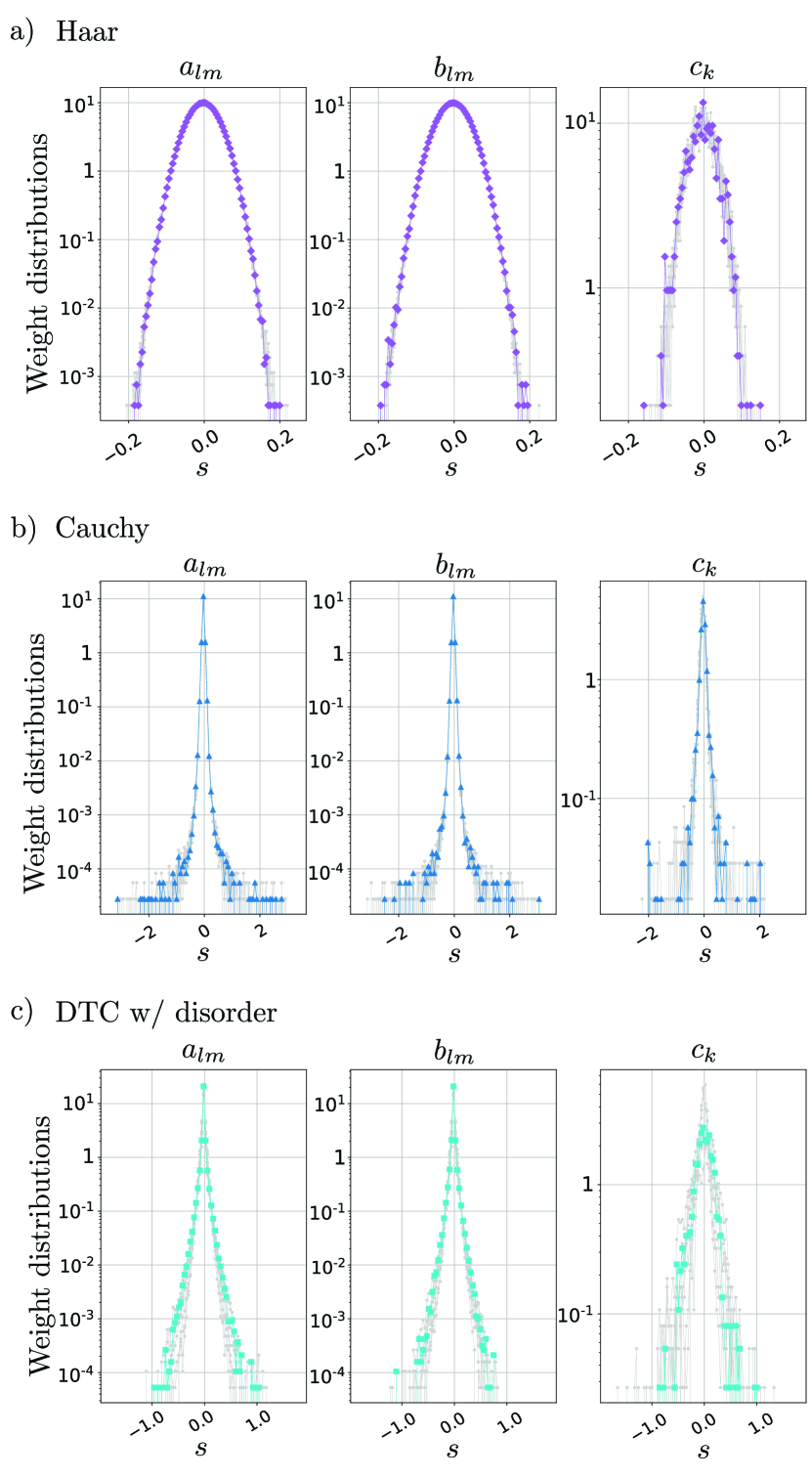
Figure 5: Weight distributions of the Haar random model a), the Cauchy random model b) and the disordered DTC model c). The total number of realizations in each case is 10. The colored curves are corresponding to each curve in Fig. 3 a,b,d) respectively. The others realizations are plotted as gray curves.

Appendix A Realization-averaged accuracy rates

In Fig. 5, we showed that the weight distribution of each model is depicted with ten realizations. The colored curves here correspond to those in Fig. 3 a,b,d). We clearly observe that the width and tail properties of the weight distribution are not strongly dependent on the particular realizations.

The realization-averaged accuracy rates for the Haar-random, Cauchy-random, and disordered DTC models are also shown in Table. 2. As the mean difference $\Delta_{\text{acc.}}$ shows, the models which have a tail in the weight distribution potentially avoid overlearning. The disordered DTC model achieves the highest generalization performance.

Average	testing (std.)	training (std.)	$\Delta_{\text{acc.}}$
Haar	0.9657 ($\pm 0.0011$)	0.9947 ($\pm 0.0003$)	0.0290
Cauchy	0.9678 ($\pm 0.0013$)	0.9943 ($\pm 0.0002$)	0.0265
DTC w/ disorder	0.9668 ($\pm 0.0005$)	0.9910 ($\pm 0.0002$)	0.0242

Table 2: Realization- and epoch- averaged accuracy rates of the various models. The epoch-average involves from 250 to 300 epochs. The realization-average is taken over 10 realizations for each model with the means (and standard deviations in parenthesis) shown. $\Delta_{\text{acc.}}$ denotes the difference between the means for training and testing.