INTRIGUING REVELATIONS FROM LITHIUM, BERYLLIUM, AND BORON

Abstract

This is a report on some highlights of research on the rare light elements, lithium (Li), beryllium (Be), and boron (B), that I presented in my Henry Norris Russell Lecture in January, 2020. It is not a comprehensive review of work on these light elements, but contains sections on Big Bang nucleosynthesis of Li and the rarity of these light elements. It includes information on how they are observed, both historically and currently, and the difficulties entailed in determining their abundances. The production of Li, Be, and B is ongoing so the youngest stars contain the most Li in their atmospheres, and they have had less time to destroy it. All three elements are readily destroyed in stellar interiors, but have differing degrees of susceptibility to the particular nuclear fusion reactions which deplete their surface content. This feature makes them remarkably good probes into the otherwise unobservable interiors of stars and provides insights into internal mixing processes. It also enhances the use of two or more of the three in sorting out the various processes at work in the insides of stars.

1 INTRODUCTION

Jesse Greenstein introduced me to the delights of stellar spectroscopy during a summer job at Caltech before my graduate school days at the University of California at Berkeley. We were studying the Ba II star, $\zeta$ Cap, which was rich in spectral lines of many rare earth elements. This interest continued through a UCB graduate course taught by George Wallerstein where I did a term paper on the rare light elments. My first published research project was an attempt to determine the Li isotope ratio in two Hyades F dwarfs; there was no clear evidence of ⁶Li (Merchant et al. 1965). George Herbig, my mentor and Ph.D thesis advisor, guided me through a research project on Be in F and G dwarfs (Merchant 1966). He called my attention to the strong Li features in M giants and supergiants which evolved into my thesis research. Lithium was present in all the 58 stars we studied at high dispersion but showed a large range of 250 in Li abundance in those cool evolved stars (Merchant 1967). This range could be attributed in part to the dilution of the surface Li as the outer convection zone deepened in evolved giant stars as had just been proposed by Iben (1965).

In the course of my post-doctoral fellowship at Caltech with Jesse Greenstein, I moved up the periodic table and studied the isotopes of Mg in 10 cool stars via the MgH features (Boesgaard 1968). Work on the Ti/Zr ratio, even further along on the periodic table, on cool stars was completed then (Boesgaard 1970a). But Li was not forgotten in work on Li in heavy metal stars and with it was the discovery of the super Li-rich S star, T Sgr (Boesgaard 1970b).

In 1967 I accepted a position as an Assistant Professor at the University of Hawaii (UH). Work on constructing the NASA-funded 88-inch (2.2m) telescope was underway at that time on Mauna Kea and it was ready for spectroscopic work in 1969. The superior quality of Mauna Kea for astronomical observations became clearly apparent in site surveys before the site selection and in subsequent astronomical work. The NASA Planetary Patrol photographs from the 24-inch telescope on Mauna Kea produced the finest images of all the comparable telescopes placed at observing sites around the world. By 1979 there were dedications of three more significant telescopes on Mauna Kea: Canada-France-Hawaii Telescope (3.6 m), NASA Infrared Telescope (3m), and United Kingdom Telescope (3.8 m). By the 1990s there were four still larger telescopes: the two 10-m Keck I and Keck II telescopes, the 8-m Subaru Japanese National telescope and the AURA 8-m Gemini North telescope. No telescopes have been placed on the actual summit of Mauna Kea, the highest point in the Pacific Ocean.

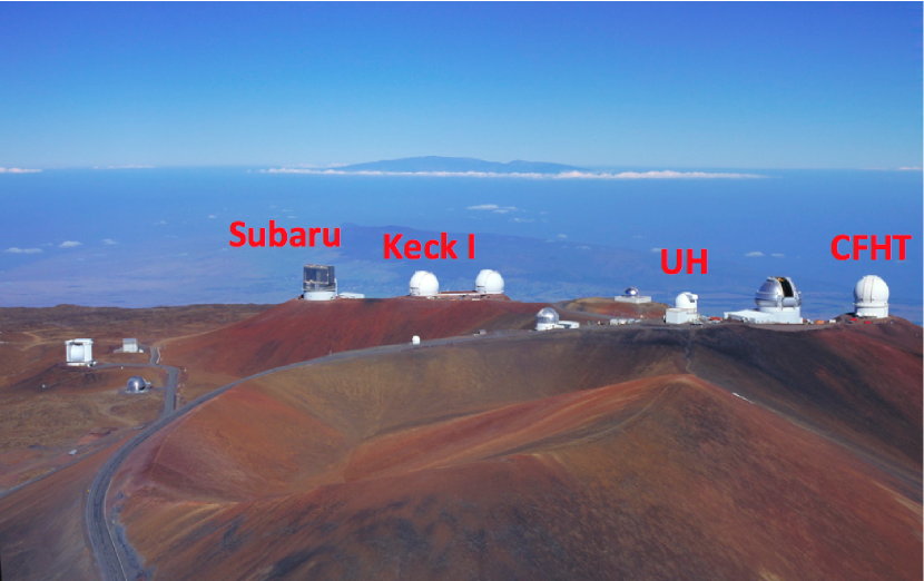
Figure 1: The Mauna Kea observatories showing the domes of the optical, infrared and sub-millimeter telescopes. The telescopes labeled are the ones used for this work. The astronomy precinct is 525 acres located within the 11,228 acre science reserve at the top of this massive mountain. The actual summit of Mauna Kea can be seen in the foreground on the right - in front of the UH dome - in this aerial view. That summit itself is free of any telescopes. The island of Maui with its ring of trade wind clouds can be seen in the distance with the summit of Haleakala. Original photograph taken by R. J. Wainscoat.

Figure 1 shows an aerial photograph of the top of Mauna Kea. The four telescopes with which I took most of my spectra for work on the light elements are labeled. Mauna Kea is a massive mountain extending 14,000 ft (4200 m) above sea level and 17,000 ft below the surface of the Pacific Ocean. Mauna Kea is the best observing site on the planet for multiple reasons. Many are due to its location far from any land mass in the middle of the ocean: dark skies, clean air, with almost no light pollution. Honolulu is below the horizon. Its high elevation puts it above the inversion layer resulting in clear skies, low humidity and low water vapor. The weather is good year round and the nighttime hours are long year round. The astronomical seeing is exceptional. In addition the low latitude of the site at +20 N means that nearly all of the sky can be observe from Hawaii. The Mauna Kea Science Reserve is an area of 11,288 acres near the summit and the “Astronomy Precinct” is a small part of that at 525 acres.

2 BIG BANG NUCLEOSYNTHESIS PRODUCES ⁷Li

In a hot Big Bang Universe nucleons are a trace component among photons and neutrinos. The epoch of nucleosynthesis begins with the formation of the hydrogen isotope, ²H, then ⁴He, followed by ³H and ³He at the expense of the neutrons. The formation of these nuclei can be seen in Figure 2 starting with the protons and neutrons at the left.

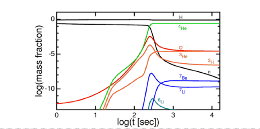
Figure 2: Element synthesis in the first 15 minutes after the Big Bang, showing the mass fraction of each component with time in seconds. (This figure is based on data from Burles, Wollett & Truran (1990) and created by E.L. Wright at UCLA).

In addition some ⁷Li is formed during this element synthesis. The amount of ⁷Be that does form decays into ⁷Li. The reactions are shown pictorially in Figure 3. So H, He, and some Li are formed in the Big Bang, but nothing else. It is important for the rest of the history of the universe – and for us – that there is no stable mass 5 and no stable mass 8. Mass 5 would result from the fusion of a H nucleus with a helium nucleus. Mass 8 would occur from the fusion of 2 He nuclei, but ⁸He decays back to 2 He nuclei. (The exception is inside stars when the temperature is hot enough to fuse that ⁸He nucleus immediately with ⁴He to make an excited state of ¹²C in the triple-alpha process.)

The periodic table of the elements shows how very different the universe is today. Once stars are formed more elements were created. It is the synthesis of the elements in stars that gets the universe from the Big Bang to today. Hydrogen and helium still dominate by orders of magnitude. They are followed by C, N, and O, completely skipping over Li, Be, and B.

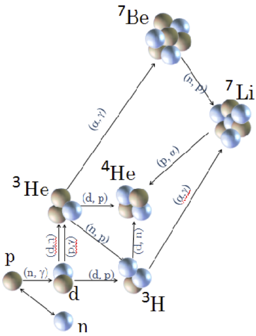
Figure 3: Nuclear reactions that occur with protons and neutrons in the first 15 minutes of the Universe. It shows how ⁷Li is formed as well as the decay of ⁷Be to ⁷Li.

3 LITHIUM, BERYLLIUM AND BORON AND THEIR RARITY

A significant and far-ranging research paper was produced by Burbidge, Burbidge, Fowler & Hoyle (1957), commonly known as B²FH, on the “Synthesis of the Elements in Stars.” They characterized element formation by several processes: H-burning, He-burning, $\alpha$-process, e-process, s-process, r-process, p-process, and the x-process. There the x-process, where the x stands for “unknown,” was for the light elements, Li, Be, and B. One example of the distribution of elements in the Sun/solar system by Anders & Grevesse (1989) is shown in Figure 4. This demonstrates clearly how rare those three light elements are relative to their neighbors on the periodic table: H and He on the low side and C, N, O all the way past Fe on the heavier side.

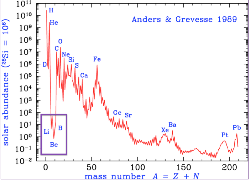
Figure 4: Solar/solar system abundance distribution by atomic mass from Anders & Grevesse (1989). The light elements Li, Be, and B, seen at the left, are very low in abundance compared to their neighbors. Data from Anders & Grevesse (1989).

A process to create Li, Be, B could not be sustained by nuclear fusion reactions inside stars. The light elements could be formed there but would be destroyed there and in the cooler, upper layers of the star, $\sim$2.5 x 10⁶ K for Li, $\sim$3.5 x 10⁶ K for Be and $\sim$5 x 10⁶ K for B. Another environment was required. An early possibility was in the interstellar gas where energetic protons and neutrons bombard abundant atoms of C, N, O and break them into smaller pieces including Li, Be and B. This mechanism was first proposed by Reeves, Fowler & Hoyle (1970) and required energies of 150 Mev or more; it is referred to as Galactic Cosmic Ray (GCR) spallation. More specific details are found in Meneguzzi, Audouze & Reeves (1971).

Inasmuch as these elements are so rare, they need to be observed in their resonance lines. However, for Li this is the Li I doublet at 6707.7 and 6707.9 Å. The ionization potential for Li I is 5.39 eV which means that for almost all stars most Li is in the form of (unobservable) Li II with resonance lines in the extreme ultraviolet. It also means that even the 6707 Å resonance doublet of Li I can be weak in solar-type stars. For Be I the resonance line is in the near UV at 2349.6 Å so it is the Be II resonance doublet that we use at 3130.4 and 3131.1 Å. The ionization potential of Be I is 9.32 so most of the Be is in the form of Be II in solar-like stars. The strongest B lines are in the satellite ultraviolet so the spectrograph needs to be above the Earth’s atmosphere. Although most of the B is in the form of B II in stars like the Sun, we observe it primarily as B I at 2497.7 Å. Observations have been made of the B II resonance at 1362.5 Å (e.g. Boesgaard & Praderie 1981) and some have been made of B III at 2066 Å (e.g. Mendel et al. 2006).

4 OBSERVING THE LIGHT ELEMENTS

4.1 Lithium

The easiest of the three light elements to observe is Li. The Li I resonance doublet is in the red region of the spectrum at 6707.76 and 6707.91 Å and relatively free of other spectral features. Only the coolest stars have blending lines of molecules such as TiO and CN. A labeled example of the Li spectral region in an F9 star in NGC 752 is shown in Figure 5 from Boesgaard et al. (2022). The strong neighboring lines are due to Fe I. The Fe I feature that is just shortward of the Li I doublet must be taken into account in determining the Li abundance, especially in cooler stars where it grows stronger. The line list used for the Li I doublet should include hyperfine structure and possibly the presence of the isotopic lines of ⁶Li and the Fe I line at 6707.4 Å. Stellar rotation can cause broadening of the line profile and needs to be taken into account, especially in rapid rotators.

Examples of spectrum synthesis fits covering the same 8 Å segment of Li are shown in Figure 6 for two Hyades stars. The synthesis fit includes the three prominent lines of Fe I; the weak blending Fe I line can be discerned in the fit at 6707.4 Å. (This Figure is from Boesgaard et al. 2016.)

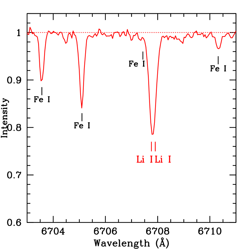
Figure 5: Eight Å in the Li I spectral region showing the Li I doublet and neighboring Fe I lines. This is an F8 dwarf star, T = 6280 K, in NGC 752. Similar to Figure 3 from Boesgaard, Lum, Chontos, et al. 2022).

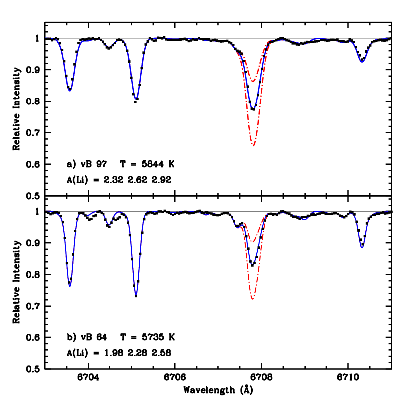
Figure 6: Examples of a spectrum synthesis fit in the Li region for two Hyades stars. The black dots are the observations and the solid blue line shows the best fit Li abundance. The red dashed-dotted lines show a factor of two more and a factor of two less Li. (Similar to Figure 9 from Boesgaard, Lum, Deliyannis et al. (2016).

4.2 Beryllium

Although Be II can be observed in stars from ground-based observatories, the resonance doublet lines at 3130.422 and 3131.067 Å are near the atmospheric cutoff ($\sim$3000 Å.) The atmospheric transmission at those wavelengths is poor and atmospheric refraction effects must be taken into account during the observations. In addition, this is a very crowded region in the spectra of F-type and cooler stars. Figure 7 shows an 8 Å region of spectra in the vicinity of the Be II lines; a few of the blending lines are identified. The line-crowding is evident in this section of spectrum, especially in comparison to Figure 5 of Li I. Both the Li figure and the Be figure show a segment of 8 Å.

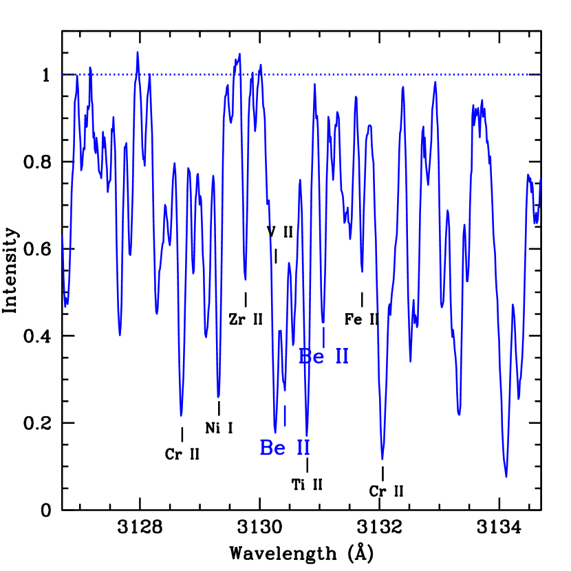
Figure 7: Eight Å in the Be II spectral region showing the Be II doublet and identifying some of the neighboring lines. This is the same star as shown for the Li region in Figure 5. Unlike the Li I region, this spectral region is very crowded with lines of atoms and molecules; only 8 Å is shown. Similar to Figure 2 from Boesgaard, Lum, Chontos et al. (2022).

Examples of the synthesis of 2 Å in the Be II region for two field stars with similar temperatures are shown in Figure 8. There are over 300 atomic and molecular lines used in the spectrum synthesis spanning the 3 Å region.

Although for metal-poor stars most of the blending lines in the Be II region are weaker, the lines due to the electronic transition lines of the OH molecule are stronger and [O/Fe] is larger. Those OH features must be taken into account and the abundance of O needs to be determined through the spectrum synthesis. Examples of this process and results are shown in Figure 9 for a star with [Fe/H] = $-$1.0 and one with [Fe/H] = $-$2.8. The abundances of both Be and O can be determined for these metal-poor stars. Three of the OH lines are shown in that region of the syntheses as labeled in the figure caption.

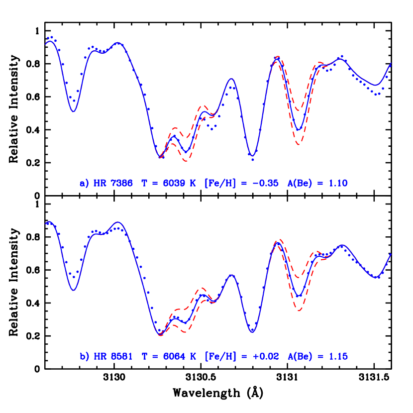
Figure 8: Synthesis of 2 Å in the Be II spectral region of two field stars. The black dots are the observations and the blue line is the best synthetic fit. The dashed red lines are a factor of 2 more and a factor of 2 less Be. From Figure 2 in Boesgaard, Armengaud, King et al. (2004b).

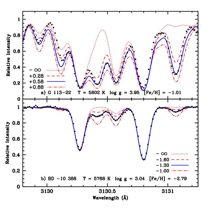
Figure 9: Synthesis of 1.45 Å in the Be II region of two metal-poor stars with similar temperatures but very different metallicities. The black squares are the observations and the solid blue lines are the best fits for Be and O. Abundances of Be are shown as a factor of two greater - dot-dashed line - and a factor of two lower - long-dash line and also a version with no Be at all as the red dotted line. Four values for the O abundance are shown differing by 0.2 are shown for the OH features at 3129.94, 3130.13, and 3130.57 Å. This is from Figure 2 from Boesgaard, Rich, Levesque et al. 2011.

4.3 Boron

Of these three light elements B is most difficult to observe because the resonance lines of the three common ions occur in spectral domains visible only above Earth’s atmosphere. Most recent observations have been made with spectrometers aboard the Hubble Space Telescope. The feature in the spectrum of B that is usually observed is the resonance line of B I at $\lambda$2496. Figure 10 shows a 2.6 Å section of four field stars showing the position of the B I line. The stars have a range in temperature of almost 500 K.

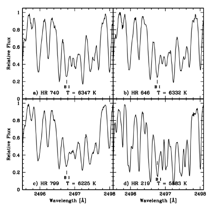
Figure 10: Examples of B spectra for four field stars at the specified temperatures observed with STIS/HST at spectral resolution of 114,000. The B I line is indicated for each star. (Figure from Boesgaard, McGrath, Lambert & Cunha 2004.)

The spectrum is very crowded which presents a challenge to extract a B abundance even with sophisticated spectrum synthesis techniques and line lists. Examples of the synthesis fits are shown for two stars in Figure 11.

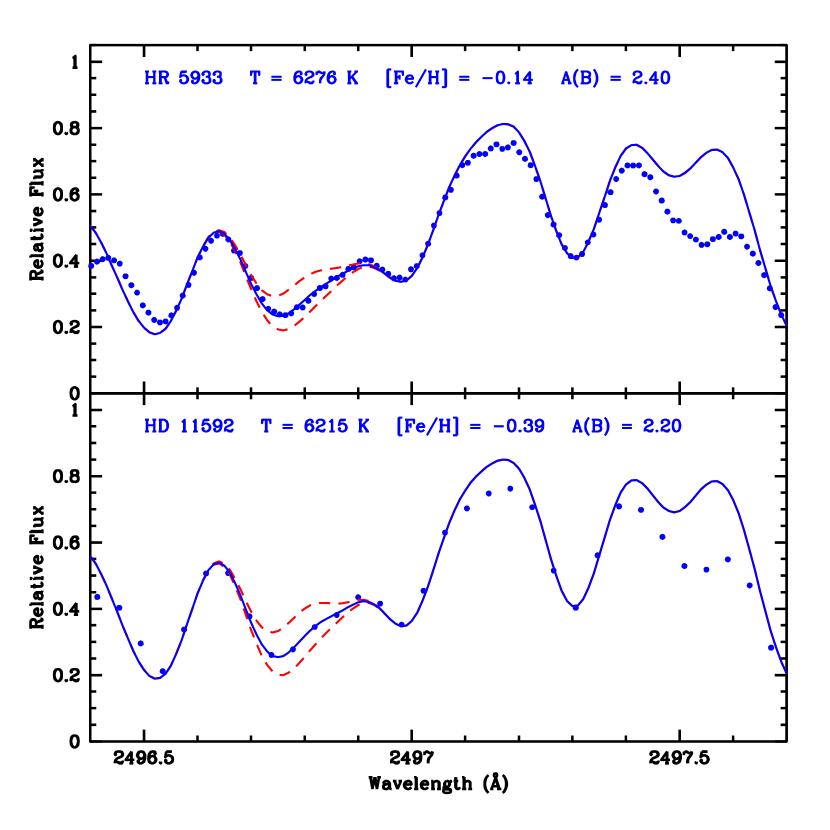
Figure 11: Spectrum synthesis of B I of HR 5933 and HD 11592. The spectrum of HR 5933 has a resolution of 114,000, while that of HD 11592 has a resolution of 30,000. The dots are the observed points and the solid line shows the best fit. The dashed lines show B abundances a factor of two higher and lower. The two stars have similar temperatures, but HD 11592 has a lower metallicity and a lower abundance of B. (Figure from Boesgaard, McGrath, Lambert & Cunha 2004.)

4.4 Effects of Stellar Rotation

Any amount of spectral line broadening increases the difficulty of determining accurate abundances. The largest amount is due to stellar rotation which is measured as v sin i. This issue is illustrated in Figure 12, left, with the synthesis fits for two Hyades stars. The observed spectra have high spectral resolution and high signal-to-noise ratios so Li abundance determinations are very good for both stars. The difference in the line-broadening is obvious with the sharp-lined star, vB 62, with v sin i = 4.8 km s^-1 and the star with broader lines, vB 121, at v sin i = 15.9 km s^-1 (The v sin i values are from Mermilliod, Mayor & Udry (2009).

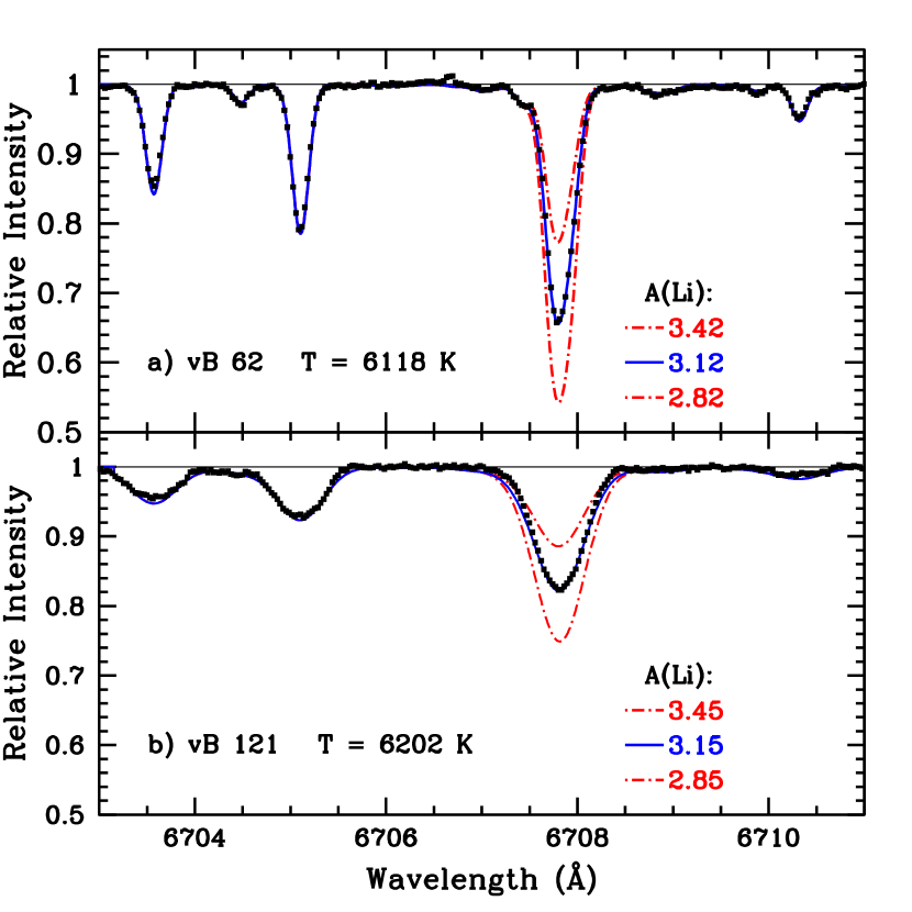
Figure 12: Left: Spectrum syntheses for Li in two Hyades dwarf stars. The upper one, vB62, has v sin i = 4.8 km s^-1 while the lower on, vB 121 has v sin i = 15.9 km s^-1 (Mermilliod, Mayor & Udry (2009). The best fit to the observed (black) points is the solid blue line. The red dash-dot lines are a factor of two higher and lower in Li. Right: Spectrum synthesis for Be in two other Hyades dwarf stars. The points are the observed spectra. The syntheses show a best fit (solid line) and a factor of two higher and lower than that fit (dotted lines). For vB 81 shown in the upper panel, the value of v sin i is 24.5 km s^-1 and for vB 66 in the lower panel v sin i is 10.2 km s^-1 (Mermilliod, Mayor & Udry (2009).

The determination of reliable results for both Be and B is dramatically impacted by the effects of stellar rotation. The resonance lines of Be II and B I occur in regions of the spectrum with many, many blending lines. Those lines all become blurred and the Be and B lines are less distinct. This can be seen in the eight Å region of Be II in Figure 7 and the six Å region of B I in Figure 10. So it is crucial to know the atomic properties of those blending lines with precision. Even so, extracting accurate values in rotating stars is extremely challenging. Figure 12, right, shows the difficulty for Be with two Hyades stars. For vb 81, with v sin i = 24.5 km s^-1, the lines are very blended by rotation. Even vB 66 with v sin i = 10.2 km s^-1, the line-broadening is troublesome. (The Be synthesis fits in Figure 8 are for stars with v sin i values of $\leq$6 km sec^-1.)

5 GALACTIC PRODUCTION AND EVOLUTION OF THE LIGHT ELEMENTS

5.1 Lithium

The present-day evidence of the Big Bang Li production was discovered in 1982 by Spite & Spite (1982) who found nearly constant Li abundances in the metal-poor stars they were studying and plotted them against temperature. Rebolo et al. (1988) displayed the Li abundances with [Fe/H] in many stars. This showed not only the constancy of Li at A(Li) at $\sim$$-$2.2 below [Fe/H] of $-$1.0 as the result of that primordial Li production, but also, at higher metallicities, both the galactic production of more Li and its destruction in individual stars. A(Li) = log N(Li)/N(H) + 12.00.

Figure 13: The relationship between the abundances of Li and Fe similar to Figure 6 from Ryan, Kajino, Beers et al. (2001). The “Li plateau” from Big Band Li production in the metal-poor dwarf stars extends from [Fe/H] near $-$4 to $\sim$$-$1.0. Some stars in the plateau region are clearly severely Li depleted. There is a strong rise in Li abundances seen at higher metallicities due to overall galactic production of the light elements. There is also severe Li depletion in many of the more metal-rich stars resulting from internal mixing processes and subsequent Li depletion.

Figure 13 is similar to Figure 6 in Ryan, Kajino, Beers et al. (2001) and shows Li abundances with [Fe/H] from $\sim$$-$4.0 to $\sim$0.0. Almost all of the stars with [Fe/H] below about $-$1.0 have the Li that was produced during the Big Bang. A few of metal-poor stars show Li depletions with only upper limits on the Li abundances. In this figure the metal-richer stars, ([Fe/H] $\geq$$-$0.4), show both galactic enhancements from light element production (e.g. GCR spallation) and stellar depletions of Li from internal mixing. Additional Li results at even lower values of [Fe/H], down to $-$6, can be found in Bonifacio et al. (2018), Aguado et al. (2019).

5.2 Beryllium and Boron

There is no expectation of primordial production of Be or B so no such plateaus with [Fe/H] were expected nor found. Both elements show a smooth enhancement with increasing Fe. This can be seen for Be in Figure 14 based on work from Boesgaard et al. (2011), supplemented by abundances from Boesgaard & Novicki (2005, 2006) and Boesgaard & Hollek (2009) primarily from Be data obtained with the Keck I high-resolution spectrograph. This covers a range in [Fe/H] of 4 orders of magnitude from $-$4.0 to 0.0 and shows a steady increase in A(Be) from $-$2.0 to +1.4 with a slope of 0.86 $\pm$0.02.

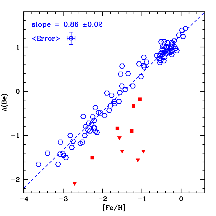
Figure 14: The counterpart diagram to Figure 13 for Be. There is no evidence for early production of Be in the Big Bang (the ⁷Be decays to ⁷Li), but the uniform Galactic production of Be with metallicity/age can be seen all the way to solar metallicity stars. The Be-deficient stars - red squares and triangles (upper limits) - are all ultra Li-deficient.

It can be seen in Figure 13 that there are some old, metal-poor stars with large Li deficiencies, i.e. stars well below the Li-plateau level for stars with the Big Bang Li. Boesgaard (2007) studied Be in seven of the nine very Li-deficient stars and found large Be-deficiences as well. Predictions from models with rotationally-induced mixing of Pinsoneault et al. (1992) do not deplete enough Be to account for the low levels of observed Be. The lack of both Li and Be could be attributed to mass transfer events or stellar mergers in binary stars which would cause mixing of material to deeper layers in the star. Such deep mixing would result in destruction of more Li and Be.

Figure 15 shows the B abundances with [Fe/H] in Duncan et al. (1997) and Duncan et al. (1998) in metal-poor stars. These observations came from the Goddard High-Resolution Spectrograph on the Hubble Space Telescope. Their sample of 12 stars covers a range of 3 orders of magnitude in [Fe/H]. The B abundance, as corrected for non-local thermodynamic equilibrium effects (nLTE) , also increases over 3 orders of magnitude. The slope of the relation is 0.96 $\pm$0.07.

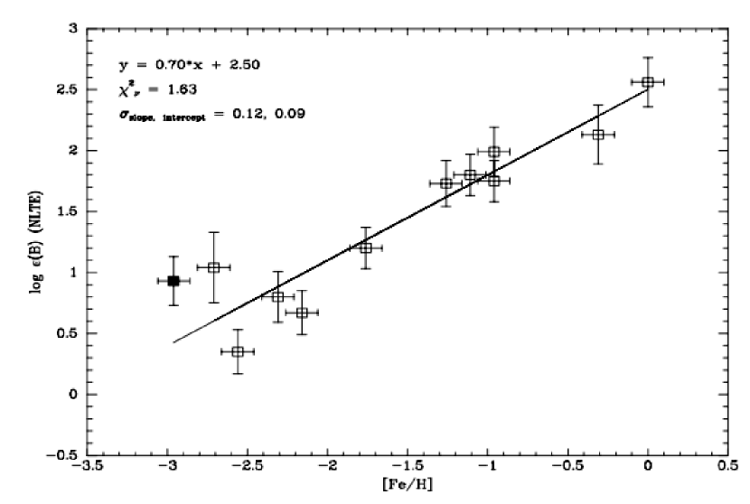
Figure 15: The relationship between the nLTE B abundance and metal content from Duncan, Primas, Rebull et al. (1997) and Duncan, Rebull, Primas et al. (1998). The slope is 0.71.

For both Be and B the abundances are done with spectrum synthesis fits. For both elements this is easier in metal-poor stars because the blending lines are all much weaker than in solar metallicity stars. As mentioned above for Be it is necessary to evaluate the O abundance also due to the larger ratio [O/Fe]. (See Figure 9.)

5.3 Abundance Evolution with Time

Boesgaard et al. (2011) determined Be abundances along with O, Ti, Mg and Fe in a sample of 117 metal-poor stars covering more than three orders of magnitude in [Fe/H]. They found a steady increase in A(Be) with [O/H] as shown in their Figures 11 and 12. Inasmuch as Li, Be, and B can be produced by energetic cosmic-ray spallation on elements like O in the interstellar medium, this connection was to be expected. Their Figure 13 also showed a rather monotonic increase in [O/H] with [Fe/H] with a slope of 0.75 $\pm$0.03 over more than two and a half orders of magnitude in [O/H]. The increases in al of those abundances is attributable to the various processes of galactic chemical evolution.

In addition, their stars could be classified by their kinematics – galactic rotation velocity and apogalactic distance – into components of the Galaxy. There were equal numbers from the dissipative collapse population and from an accretion-process population. But the relationship between A(Be) and [Fe/H] and between A(Be) and [O/H] were different for those two populations. For the dissipative group the slopes were near 1: 0.94 $\pm$0.04 for Be with Fe and 1.13 $\pm$0.08 for Be with O. For the accretive population the slope between A(Be) and [Fe/H] was 0.68 $\pm$0.04. For A(Be) and [O/H] it was 0.76$\pm$0.06. The accretive stars demonstrated a slower increase in Be relative to both Fe and O than the classical disk and halo stars.

6 STELLAR INTERIORS and LIGHT ELEMENT DESTRUCTION

6.1 Open Clusters

Wallerstein, Herbig & Conti (1965) studied Li in the Hyades with spectra from photographic plates. They measured line strengths of Li I at 6707 Å and 7-12 lines of Ca I and determined the ratio of [Li/Ca] for 23 main sequence stars. They found a decline with increasing B-V, i.e. decreasing temperature. For most of the hotter stars they could find only upper limits on the Li abundances because the stars were rotating rapidly and the lines were too broad for reliable line measurements. The decline in Li was further defined by Zappala (1972) with Li determinations in 41 Hyades FGK stars. With high quality reticon spectra from the CFHT coudé spectrograph of 12 Hyades stars cooler than 6000 K, Cayrel et al. (1984) determined that the decline with temperature was even steeper than found in those prior studies.

Then Boesgaard & Tripicco (1986) obtained high signal-to-noise spectra with a reticon detector at the CFHT coud/’e spectrograph and with a CCD detector at the UH 2.24-m telescope coud/’e spectrograph of Hyades stars in the temperature range 6000 - 7100 K. They found a dramatic drop in Li abundances in stars near 6500 K with A(Li) more than 2 orders of magnitude lower than in stars 300 K hotter or cooler. Figure 16, left, shows the modern version of Li in the Hyades with the F dwarf Li dip and the G dwarf Li fall off. (Data from Boesgaard, Lum, Deliyannis et al. 2016.)

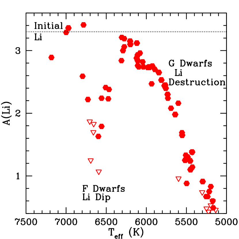
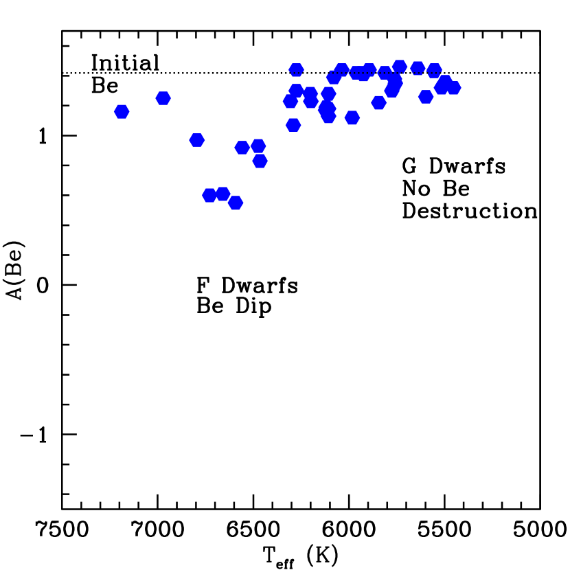
Figure 16: Left: The distribution of Li abundance with temperature in the Hyades showing the deep Li depletions in the narrow temperature range centered near 6600 K and the dramatic decline in Li with decreasing temperature for stars cooler than $\sim$6100 K. Right: The distribution of Be abundance in the Hyades revealing a much shallower Be depletion in the mid-F dwarf stars and no change in the Be abundance for the cooler stars. Data are from Boesgaard, Lum, Deliyannis et al. (2016).

This result prompted both theoretical explanations of the Li dip and more observations of Li in this temperature regime in other open clusters. The most interesting additional cluster to be observed was the (younger) Pleiades which had little or no Li dip (see below).

A first attempt to determine Be in the Hyades stars was done by Boesgaard & Budge (1989) for eight stars. Later observations were made of Be in 34 Hyades stars with HIRES on Keck I by Boesgaard & King (2002). They discovered evidence for a Be dip that was similar but not as deep as the Li dip. They also found that there was no decline in Be in the cooler stars as was found for Li in the Hyades. The modern version of this result is shown in Figure 16, right. The Be observations were well-matched by models with rotationally-induced mixing below the convection zone by Deliyannis & Pinsonneault (1997). Figure 10 in Boesgaard & King (2002) shows the Hyades Be results with effective temperature and those model fits with initial rotation values of 10 and 30 km s^-1. Their Figure 11 shows the same results for Li.

The observational results for for both Li and Be in the Hyades are shown together as a function of stellar surface temperature in Figure 17, left, on the same scale and normalized to their respective solar system abundances.

Observations of both Li $\underline{and}$ Be in 24 field stars with temperatures between 5700 and 6700 K led Deliyannis et al. (1998) to the finding that Li and Be were rather tightly correlated with a slope of about 0.4. This enabled them to exclude some of the explanations that had been proposed for the Li (only) depletions. For example, with mass loss accounting for the Li depletion, all the Li would be lost before any effect would be seen on Be. With microscopic diffusion, which would affect the two elements similarly, the slope would be close to 1. The models of Deliyannis & Pinsonneault (1993, 1997) and Charbonnel et al. (1994) involved slow mixing caused by the effects of stellar rotation and provided an excellent fit to the data. This showed the importance of having abundances of two (or more) of the light elements for the interpretation of the depletions of the light elements. It demonstrated that the depletions were occurring simultaneously.

An important insight about this Li dip came from the study of Li in the young Pleiades by Pilachowski, Booth & Hobbs (1987) and Boesgaard, Budge & Ramsey (1988) who also included stars in the young $\alpha$ Per group. There was no Li dip as found in the mid-F dwarfs in the Hyades. This showed that the mechanism which caused the large depletion seen in the Hyades was a main-sequence phenomenon and not a pre-main sequence occurrence.

If there were no Li depletion in the Pleiades, no Be depletion was to be expected. Boesgaard, Armengaud & King (2003a) studied Be in the young clusters Pleiades and $\alpha$ Per. Figure 17, right, reveals the combined Li and Be results for the young Pleiades, again scaled and normalized as Figure 17, left, along with the fit through the Hyades Li data. With an age of $\sim$650 Myr the Hyades exhibits a pronounced dip in Li and a well-defined dip in Be can be seen. But there is no well-defined dip in either element in the stars of the younger Pleiades at $\sim$130 Myr, a cluster one-fifth the age of the Hyades.

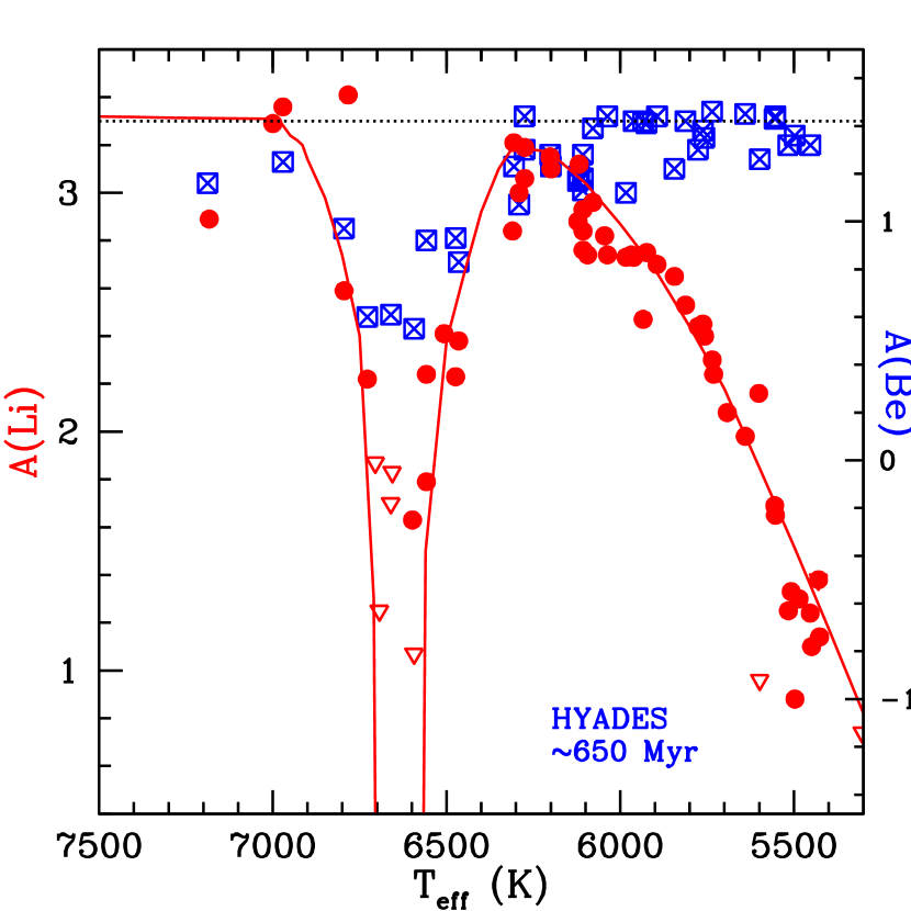
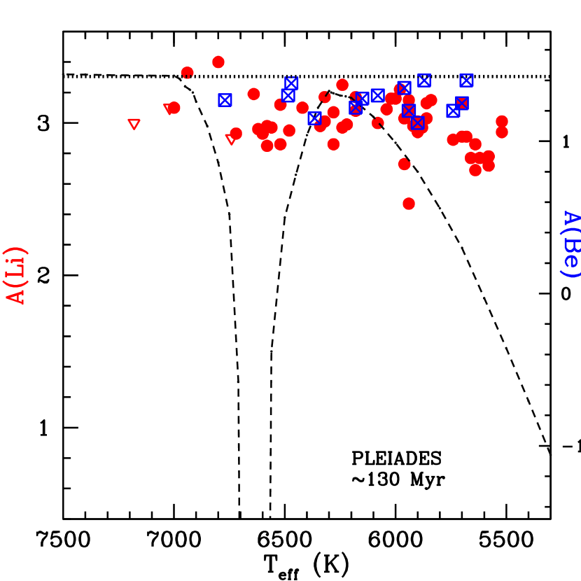
Figure 17: Left: Abundances of Li and Be on the same scale as a function of stellar temperature for the Hyades, age $\sim$650 Myr. There is some Be depletion in the 6600 K region, but not nearly as much as found for Li. There are no upper limits in the Be abundances. The steep decline in Li from T $\sim$6200 to 5300 K is not seen for Be. Right: Abundances of Li and Be on the same scale as a function of stellar temperature for the younger Pleiades cluster at age $\sim$130 Myr. There is little if any depletion of Li or Be in the younger Pleiades.

This extra internal-mixing effect - caused by rotation and spindown - showed that it was very important in depleting surface Li, but less effective for Be in the mid-F dwarf stars . An important next step was to determine the effect of this internal mixing on B. As mentioned above, B requires an even higher temperature, $\sim$5 x 10⁶ K, for thermonuclear reactions to destroy it. It is also more difficult to observe, but ultimately we were able to use the Hubble Space Telescope with its high resolution spectrograph to observe B in a few Hyades stars. The results for the Hyades can be seen in Figures 18, left, for B and Li and Figure 18, right, for B and Be. The two stars that are in the Li-Be dip in the Hyades are depleted relative to the three on either side of the dip. The dotted lines connect those B points to their respective Li and Be points. They indicate that there is a measurable depletion on B also.

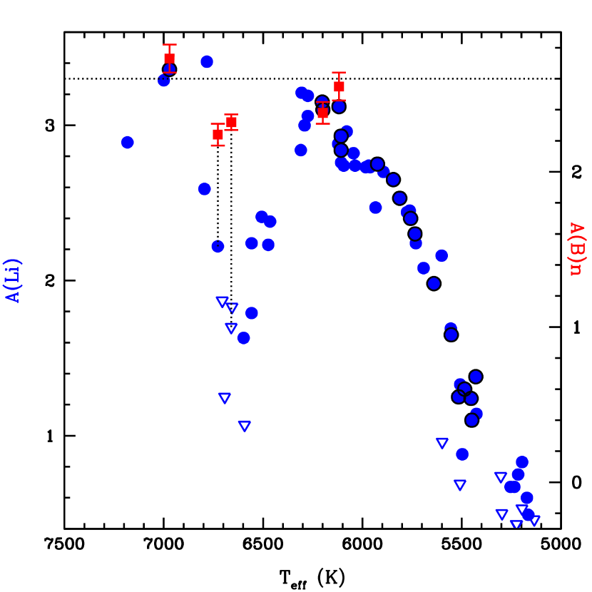
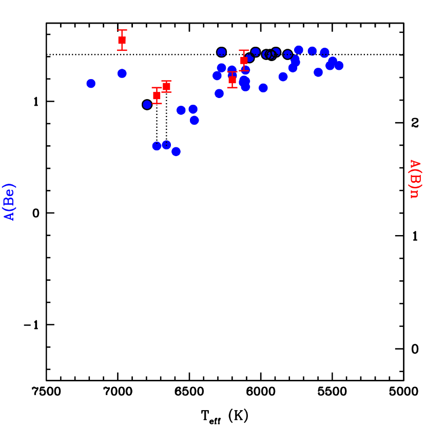
Figure 18: Abundances of Li and B on the same scale as a function of stellar temperature for the Hyades. The two Li-dip stars observed for B are depleted while the three stars outside the Li dip are not. The dotted lines connect the Li and B results for those two stars. Right: The same figure with Be and B results on the same scale. Again, the two Li-Be dip stars are seen to be B depleted; the results for those stars are connected by dotted lines.

A graphical depiction of a standard solar model is shown in Figure 19. There is an outer convection zone which is rather shallow in the Sun. The nuclei of atoms of Li have all been destroyed inside the red ring which encloses temperatures higher than $\sim$2.5 x 10⁶ K. Atoms of Be are destroyed inside the blue ring at $\sim$3.5 x 10⁶ K and those of B inside the purple ring at $\sim$5 x 10⁶ K . The surface shell which contains Li is very small while the shell with Be extends deeper in the star to higher temperatures and the shell with B is considerably larger. That is the reservoir with Li is smaller than that of Be and B and that of Be, while larger than the reservoir for Li is smaller than that for B. This diagram illustrates two of the basic issues. 1) With the deepening of the surface convection zone in main-sequence stars with decreasing surface temperatures, the amount of Li on the surface will decrease as Li atoms are mixed to deeper layers by convection. However, convection alone is not sufficient to deplete Li in the Sun. Additional mixing mechanisms must be included in the standard models. 2) The dip in the abundances of Li, Be, and B near 6600 K can not be understood by standard models either, but the relative size of the depletions there are determined by the susceptibility to thermonuclear destructive reactions of each of the three elements.

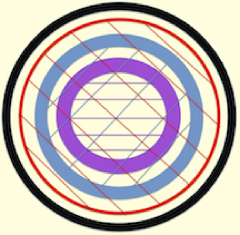
Figure 19: A schematic image of a solar mass star. Lithium nuclei are destroyed inside the red circle with red diagonal lines, where the temperature is hotter than $\sim$2.5 x 10⁶ K. Beryllium nuclei are destroyed inside the blue circle with blue diagonal lines at $\sim$3.5 x 10⁶ K and B nuclei are destroyed inside the purple circle with purple horizontal lines at $\sim$5 x 10⁶ K. The black outer circle depicts the surface convection zone in the Sun which does not penetrate deeply enough to mix the surface layers to temperatures where the light elements would be destroyed.

6.2 Correlation of Light Element Depletions

Further observations of both Li and Be in main-sequence cluster stars and in field stars showed how well-correlated the abundances of these two elements are. We studied Be in the young clusters Pleiades and $\alpha$ Per (Boesgaard, Armengaud & King (2003a), in the older Coma cluster and UMA Moving Group (Boesgaard, Armengaud & King (2003b), and in Praesepe and other clusters (Boesgaard, Armengaud & King (2004a) and put it together with field stars in Boesgaard, Armengaud & King (2004b). These results provided a much larger sample in which to investigate the correlation of Li and Be. This can be seen here in Figure 20, left, for stars on the cool side of the Li-Be dip, T = 6000 - 6650 K. The relationship has a slope of 0.44 $\pm$0.05. This is a remarkable relationship covering a range in Li of 400 times and Be of more than 10 times for a large spread in age.

Both Be and B have been observed in field stars by Boesgaard et al. (2005) and in those five Hyades stars discussed above (Boesgaard et al. (2016). These two elements are also well-correlated. Figure 20, right, shows the Be-B relationship for stars on the cool side of the Li dip T = 6100 - 6739 K) from four Hyades stars and 14 field stars with detectable Be and B. This relationship has a slope of 0.22 $\pm$0.05. The slope is shallower than that for the Li-Be correlation (0.22 vs. 0.44) and extends over a range of 100 in A(Be) and a range of 4 in A(B). Models of stars with mixing induced by rotation match the Be to B relation as discussed in Boesgaard et al. (2016) and seen in their Figure 15.

These observations show that Li declines more rapidly than Be. They show that Be declines more rapidly than B. But we cannot compare Li and B because there is no Li left when B starts to decline.

6.3 Light Element Dilution

In evolved stars the light elements can be diluted as well as depleted. When leaving the main sequence normal FGK stars expand and their outer convection zones grow. As mentioned above, each of these light elements has its own outer shell of material which contains its ions. As a star starts to expand to become a red giant, this outer shell also expands. The matter becomes diluted by material containing no Li, Be, or B from deeper layers. The effect is first noticeable with Li as it is only in the outermost shell. Then the dilution will begin to affect Be and dilute its surface content. Finally B, with the deepest reservoir containing B ions, will become diluted also. A study of Li and Be in subgiants in the old open cluster, M 67, at 3.9 Gyr shows the effects of both depletion and dilution of both light elements (Boesgaard, Lum & Deliyannis 2020).

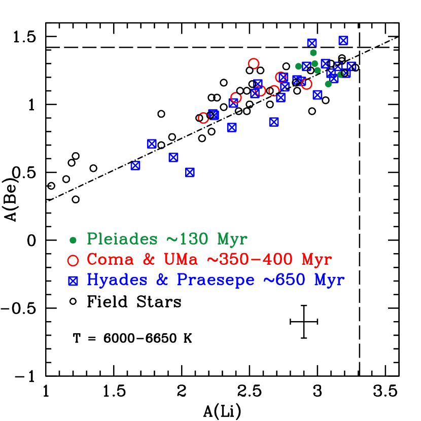
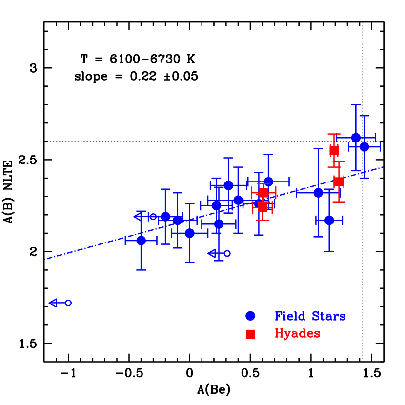
Figure 20: Left: Li and Be in main-sequence dwarfs in cluster and field stars on the cool side of the Li-Be dip region. Both Li and Be depletions have occurred, but Li is more depleted than Be. The slope of this relationship is 0.44 $\pm$0.05. The relationship spans over 200 times in Li abundance. Right: Be and B in field and cluster dwarf stars on the cool side of the Li-Be-B dip. This figure is from Boesgaard, Lum, Deliyannis et al. (2019), Figure 14. The slope is less steep than that for Li vs. Be at 0.22 $\pm$0.05. The depletion covers a range of $\sim$100 in Be abundance. There is no comparable diagram of Li and B because all the Li is destroyed before there is measurable decline in B.

7 SOME CONCLUSIONS

In spite of their very low cosmic abundances, this trio of light elements has produced some profound and interesting insights into stellar structure and evolution. The easiest to observe is Li which also provides information about Big Bang nucleosynthesis.

The low abundance, however, means that observations must be made of the strongest spectral features: the resonance lines. For Li this is the Li I 6707 Å doublet which is in an easily observable spectral region. Due to the low excitation potential of Li I, 5.39 eV, for most stars Li is in the form of Li II, however. Beryllium observations are made of the resonance doublet of Be II at 3130 Å, close to the atmospheric cutoff and in a spectral region full of blending lines. The resonance lines of B I, B II, and B III are all in the ultraviolet spectral region observable by satellite only.

Most very low-metal stars show a plateau or a maximum in Li near A(Li) of 2.2 that is a product of Big Bang nucleosynthesis. There are some, but not many, stars at those low metallicities which show no Li feature. Those ultra-Li-deficient stars that have been studied for Be turn out to have Be deficiences as well. This dual deficiency could result from stellar mergers or mass transfer events (see Boesgaard 2007).

Only in stars with [Fe/H] $\gtrsim$$-$1 are there any found with larger amounts of Li. There is a gradual increase in A(Li) with [Fe/H] in normal dwarf stars to a maximum is near A(Li) of +3.3. This results from the general galactic enrichment in Li, Be, and B over time. A large range in A(Li) of three orders of magnitude can be seen in solar type stars caused by that galactic enrichment and by the slow stellar Li destruction.

For both Be and B there is a marked and steady increase with [Fe/H]. Figures 14 and 15 show the clear increases in these elements over the course of the evolution of the Galaxy. The increase in A(Be) with [Fe/H] and [O/H] (and with [Ti/H] and [Mg/Fe]) for 117 metal-poor stars emphasizes the trend with chemical evolution (Boesgaard et al. (2011).

Some profound insights have come from the analysis of Li, Be, and B that are related stellar interiors. The surface abundances of these elements are important guides to internal mixing. The surface contents in clusters show that light element depletion is a phenomenon of main sequence evolution. The dramatic drop in Li especially, but also Be and B, in the mid-F dwarfs is apparently the result of extra internal mixing caused by rotation. The abundances of Li and Be are well correlated in main-sequence stars in clusters and in the field over a span of a factor of 400 in Li abundance. This is true for Be and B in the Hyades and in field stars as well for a range of a factor of 100 in Be.

8 ADDITIONAL COMMENTS

The classic image of the lone astronomer with his (sic) eye at the telescope is far from true in today’s world of astronomy. The tools of our trade are extremely complicated and require the talents and efforts of a genuine multitude of people. Just think of the complex business of designing and building a modern telescope which is a multi-ton machine (300 tons for the Keck telescopes) which has to track to better than 0.01 arcsec and has to operate with better than clockwork precision. It involves 24-inch I-beams down to 00 screws. Furthermore, that telescope needs sophisticated instruments to detect photons from astronomical objects. Those instruments work best when accompanied by sensitive modern detectors. And what would an astronomer do without all the software designers who make the telescope operate? And the ones who run the instruments that produce data? And those who provide technical support, even in the middle of the night? There are also those who devise the various tools that help in the analysis of that data? Even in the days of my youth when astronomers developed their own photographic plates, they relied on data reduction techniques and equipment developed by others. At that time we had graphic artists and photographers to make our plots and diagrams ready for publication.

My point here is that in order for astronomers to collect, analyze, and interpret data from a scientific program they want to pursue, they rely on virtual legions of other people. Furthermore we interact with other astronomers regarding our findings. I am extremely grateful to this collection of engineers, designers, computer experts, telescope operators, assistants, colleagues and students. Sometimes even small interactions produce big thoughts or germinate new approaches to ongoing issues. I want them to know how aware I am of all their extensive help. My deep thanks go to all the many colleagues and students I’ve worked with and who have so expanded my horizons. I dedicate this talk and paper to Hans Boesgaard, my husband, my best friend, my favorite telescope engineer.

References

- (1) Aguado, D.S., Gonzalez Hernandez, J.I., Allende Prieto, C. et al. 2019, ApJ, 874, 21
- (2) Anders, E. & Grevesse, N. 1989, GeCoA, 53, 197
- (3) Asplund, M., Grevesse, N. & Amarsi, A.M. 2021, A&A, 653, A141
- (4) Boesgaard, A.M. 1968, ApJ, 154, 188
- (5) Boesgaard, A.M. 1970a, ApJ, 161, 163
- (6) Boesgaard, A.M. 1970b, ApJ, 161, 1003
- (7) Boesgaard, A.M. 2007, ApJ, 667, 1196
- (8) Boesgaard, A.M., Armengaud, E., King, J.K. et al. 2004, ApJ, 613, 1202
- (9) Boesgaard, A.M., Armengaud, E., King, J.K. 2003a, ApJ, 582, 410
- (10) Boesgaard, A.M., Armengaud, E., King, J.K. 2003b, ApJ, 583, 955
- (11) Boesgaard, A.M., Armengaud, E., King, J.K. 2004a, ApJ, 605, 864
- (12) Boesgaard, A.M., Armengaud, E., King, J.K. 2004b, ApJ, 613, 1202
- (13) Boesgaard, A.M., Budge, K.G. & Ramsey, M.B. 1988 ApJ, 327, 389
- (14) Boesgaard, A.M. & Budge, K.G. 1989, ApJ, 338, 875
- (15) Boesgaard, A.M., Deliyannis, C.P. & Steinhauer, A. 2005, ApJ, 621, 991
- (16) Boesgaard, A.M. & Hollek, J.K. 2009, ApJ, 691, 1412
- (17) Boesgaard, A.M. & King, J.R. 2002, ApJ, 565, 587
- (18) Boesgaard, A.M., Lum, M.G., Chontos, A. et al. 2022, ApJ, 927, 118
- (19) Boesgaard, A.M., Lum, M.G., Deliyannis, C.P. et al. 2016, ApJ, 830, 49
- (20) Boesgaard, A.M., Lum, M.G.& Deliyannis, C.P. 2020 ApJ, 888, 28
- (21) Boesgaard, A.M., McGrath, E.J., Lambert, D.L. & Cunha, K. 2004, ApJ, 606, 306
- (22) Boesgaard, A.M. & Novicki, M. 2005, ApJ, 633, 125
- (23) Boesgaard, A.M. & Novicki, M. 2006, ApJ, 641, 1122
- (24) Boesgaard, A.M., Praderie, F., Leckrone, D. et al. 1974, ApJ, 194, 143
- (25) Boesgaard, A.M. & Praderie, F. 1981, ApJ, 245, 219
- (26) Boesgaard, A.M., Rich, J.A., Levesque, E.M. & Bowler, B.P. 2011, ApJ, 743, 140
- (27) Boesgaard, A.M. & Tripicco, M. J. 1986, ApJ, 302, L49
- (28) Bonifacio, P., Caffau, E., Spite, M. et al. 2018, A&A, 612, A65
- (29) Burbidge, E.M., Burbidge, G., Fowler, W.A. & Hoyle, F. 1967 RvMP, 29, 547
- (30) Cayrel, R., Cayrel de Strobel, G., Campbell, B. et al. 1984, ApJ, 283, 204
- (31) Charbonnel, C., Vauclair, S., Maeder, A. et al. 1994, A&A, 283, 158
- (32) Deliyannis, C.P., Boesgaard, A.M., Stephens, A. et al. 1998, ApJ, 498, 147
- (33) Deliyannis, C.P. & Pinsonneault, M. 1993, ASPC, 40, 174
- (34) Deliyannis, C.P. & Pinsonneault, M. 1997, ApJ, 488, 836
- (35) Duncan, D.K., Primas, F., Rebull, L.M. et al. 1997, ApJ, 488. 338
- (36) Duncan, D.K., Rebull, L.M., Primas, F. et al. 1998, A&A, 332, 1017
- (37) Iben, I., Jr. 1965, ApJ, 142, 1447
- (38) Mendel, J.T., Venn, K.A., Proffitt, C.R. et al. 2066, ApJ, 640, 1039
- (39) Meneguzzi, M., Audouze, J. & Reeves, H. 1971, A&A, 15, 337
- (40) Merchant, A.E., Bodenheimer, P. & Wallerstein, G. 1965, ApJ, 142, 790
- (41) Merchant, A.E. 1966, ApJ, 143, 336
- (42) Merchant, A.E. 1967, ApJ, 147, 587
- (43) Mermilliod, J.-C., Mayor M. & Udry, S. 2009, A&A. 498, 949
- (44) Pilachowski, C.A., Booth, J. & Hobbs, L.M. 1987, PASP, 99, 1288
- (45) Rebolo, R., Molaro, P. & Beckman, J.E. A&A, 192, 192
- (46) Reeves, H., Fowler, W.A. & Hoyle, F. 1970, Nature, 226, 727
- (47) Ryan, S.G., Beers, T.C., Kajino, T. et al. 2001, ApJ, 547, 231
- (48) Ryan, S., Kajino, T., Beers, T.C. et al. 2001, ApJ, 549, 55
- (49) Pinsonneault, M.H., Deliyannis, C.P. & Demarque, P. 1992, ApJS, 78, 179
- (50) Sneden, C. 1973, ApJ, 184, 839
- (51) Sneden, C., Bean, J., Ivans, I., Lucatello, S., & Sobeck, J. 2012, MOOG: = LTE line analysis and spectrum synthesis, Astrophysics Source Code = Library, ascl:1202.009
- (52) Spite, F. & Spite, M. 1982, A&A, 115, 357
- (53) Tody, D. 1986, SPIE, 627, 733
- (54) Tody, D. 1993, ASPC, 52, 173
- (55) Wallerstein, G., Herbig, G.H. & Conti, P.S. 1965, ApJ, 141, 610
- (56) Zappala, R.R. 1972, ApJ, 172, 57
- (57)