Unconfoundedness with Network Interference

Abstract. This paper studies nonparametric estimation of treatment and spillover effects using observational data from a single large network. We consider a model in which interference decays with network distance, which allows for peer influence in both outcomes and selection into treatment. Under this model, the total network and covariates of all units constitute sources of confounding, in contrast to existing work that assumes confounding can be summarized by a known, low-dimensional function of these objects. We propose to use graph neural networks to estimate the high-dimensional nuisance functions of a doubly robust estimator. We establish a network analog of approximate sparsity to justify the use of shallow architectures.

JEL Codes: C14, C31, C45

Keywords: causal inference, network interference, unconfoundedness, graph neural networks

1 Introduction

A large literature studies causal inference under network interference when treatments are randomly assigned. This paper considers observational settings under a high-dimensional network unconfoundedness condition. Existing work assumes confounding can be summarized by a known, low-dimensional vector of network controls, but it is unclear what model of selection justifies a given choice of controls. We propose a nonparametric behavioral model that allows for peer influence in outcomes and selection into treatment. Under this model, the total network and all unit covariates constitute sources of confounding, which motivates our unconfoundedness condition. We make the case that graph neural networks are well-suited for estimation in this setting, and we provide primitive conditions for a network analog of approximate sparsity that makes high-dimensional estimation feasible.

We begin by reviewing the conventional approach to causal inference with network interference, the assumptions of which we seek to generalize. Let $\bm{A}$ be a network of $n$ units, $D_{i}\in\{0,1\}$ be unit $i$’s treatment assignment, and $\bm{D}=(D_{i})_{i=1}^{n}$. Denote by $Y_{i}(\bm{d})$ the potential outcome of unit $i$ under the counterfactual that treatments are given by $\bm{d}=(d_{i})_{i=1}^{n}\in\{0,1\}^{n}$ rather than $\bm{D}$. Under network interference, $\bm{A}$ mediates the dependence of $Y_{i}(\bm{d})$ on $d_{j}$ for $j\neq i$.

In a single-network setting, it is necessary to impose restrictions on interference. By far the most common is neighborhood interference, which posits that a known, low-dimensional function of $(\bm{D},\bm{A})$ summarizes interference. This model represents potential outcomes as

$$Y_{i}(\bm{D})=\tilde{Y}_{i}(T_{i})\quad\text{for}\quad T_{i}=f_{n}(i,\bm{D},\bm{A}).$$ (1)

The effective treatment (Manski, 2013) or exposure mapping (Aronow and Samii, 2017) $T_{i}$ is a low-dimensional, vector-valued function of the treatments, and $\tilde{Y}_{i}(t)$ is the potential outcome of unit $i$ under the counterfactual that $i$ has exposure mapping $t$. A simple example is $T_{i}=(D_{i},\sum_{j=1}^{n}A_{ij}D_{j})$ where $A_{ij}$ is an indicator for whether $i$ and $j$ are connected in $\bm{A}$. The first component of $T_{i}$ captures the direct effect of treatment while the second captures interference induced by the number of $i$’s treated neighbors. As is the case for most specifications of $T_{i}$ in the literature, this choice implies no interference beyond the ego’s $K$-neighborhood for some known threshold $K$, in this case $K=1$.

Under model (1), a common causal estimand of interest is

$$\frac{1}{n}\sum_{i=1}^{n}{\bf E}[\tilde{Y}_{i}(t)-\tilde{Y}_{i}(t^{\prime})\mid\bm{A}]\quad\text{for}\quad t,t^{\prime}\in\mathcal{T}.$$ (2)

Depending on the choice of $f_{n}(\cdot)$, $t$, and $t^{\prime}$, this may capture an average treatment and/or spillover effect. For instance, choosing $t=(1,0)$ and $t^{\prime}=(0,0)$ results in an average treatment effect for units with no treated neighbors. Inference on (2) is well-understood because neighborhood interference induces a convenient form of network weak dependence (Aronow and Samii, 2017; Leung, 2020).

However, neighborhood interference can be restrictive. It assumes the exposure mapping is correctly specified by the econometrician, which may be a demanding requirement (Sävje, 2023). It also rules out social behavior of economic interest such as endogenous peer effects and models of diffusion (Leung, 2022a). This motivates the “approximate neighborhood interference” (ANI) condition proposed by the previous reference, which posits that interference tends to zero with path distance. It does not require precisely zero interference after some fixed and known distance $K$, in contrast to (2) under most choices of $T_{i}$ used in practice. To allow for richer forms of interference, we adopt the ANI model in this paper.

1.1 Unconfoundedness

Whereas most of the literature on interference studies randomized experiments, we consider observational data. This is a relatively recent topic of research with key contributions due to Forastiere et al. (2021) and Ogburn et al. (2022). They study estimation of (2) under neighborhood interference and the unconfoundedness condition

$$\tilde{Y}_{i}(\cdot)\perp\!\!\!\perp T_{i}\mid W_{i}$$ (3)

where $W_{i}$ is a low-dimensional vector of controls. These may include unit-level covariates $X_{i}$ that do not depend on $\bm{A}$, as well as what we might call “network controls,” which generally can be any function of the network and covariates, for example $\sum_{j=1}^{n}A_{ij}X_{j}/\sum_{j=1}^{n}A_{ij}$ or other centrality measures.

However, just as $T_{i}$ may be misspecified, so may be $W_{i}$. Given the wide range of options for constructing network controls, it may be challenging to justify that a particular choice adequately adjusts for confounding. Important recent work by Sánchez-Becerra (2022) provides a model of selection that establishes (3) for a class of exposure mappings when using controls $W_{i}=X_{i}$. Hence, there is no need for network controls in his framework. Since the previous papers do utilize network controls, this raises the question of what model of selection justifies their use.

Unlike most of the literature, we consider approximate neighborhood interference in selection into treatment (as well as in potential outcomes), which allows for peer effects in treatment take-up. Suppose, for example, that $D_{i}$ represents a worker $i$’s decision to adopt a new technology and $Y_{i}(\bm{D})$ is $i$’s productivity. Peer effects in productivity (Mas and Moretti, 2009) induce interference with respect to outcomes. Moreover, the decision to adopt new technology may be subject to peer influence (Conley and Udry, 2010), which induces “interference” in selection.

Under our model, $Y_{i}(\bm{D})$ and $D_{i}$ may depend on the entirety of $\bm{X}=(X_{i})_{i=1}^{n}$ and $\bm{A}$, so it becomes necessary to account for high-dimensional network confounding. We therefore adopt the unconfoundedness condition

$$\{Y_{i}(\cdot)\}_{i=1}^{n}\perp\!\!\!\perp\bm{D}\mid\bm{X},\bm{A}.$$ (4)

This does not require the econometrician to correctly specify a low-dimensional function $T_{i}$ of $(\bm{D},\bm{A})$ to restrict interference, as in (1), or a low-dimensional function $W_{i}$ of $(\bm{X},\bm{A})$ to summarize confounding.

Forastiere et al. (2021) and Sánchez-Becerra (2022) study semiparametric models of potential outcomes and/or treatment selection, while Emmenegger et al. (2022) take a nonparametric approach. We also study nonparametric estimation and, like Emmenegger et al. (2022), utilize a doubly robust estimator. Unlike their paper, we do not assume (3), and we specifically make the case for estimating the unknown functions using graph neural networks (GNNs).

1.2 Graph Neural Networks

We consider a generalization of estimand (2) proposed by Sävje (2023) that compares average outcomes of units with different exposure mappings without utilizing the mappings to restrict interference as in the neighborhood interference model. Under our unconfoundedness condition, doubly robust estimation requires an estimate of the generalized propensity score ${\bf P}(T_{i}=t\mid\bm{X},\bm{A})$ (Imbens, 2000). This is a nonstandard estimation problem because the input is high-dimensional and graph-structured. Additionally, we will require the propensity score to satisfy permutation-invariance, meaning that units with isomorphic positions in the network have identical propensity scores. This restriction is weaker than what is assumed in the existing literature and is required because it would otherwise be necessary to estimate $n$ unit-specific propensity scores, which is generally impossible.

We propose to use GNNs, which are exactly designed to estimate permutation-invariant functions of networks. A key parameter of a GNN is its depth, or number of layers, $L$, which determines the receptive field $(\bm{X}_{\mathcal{N}(i,L)},\bm{A}_{\mathcal{N}(i,L)})$ used to predict $i$’s outcome. For example, a one-layer GNN only uses $i$’s 1-neighborhood to predict its outcome, limiting the input used for prediction to $(\bm{X}_{\mathcal{N}(i,1)},\bm{A}_{\mathcal{N}(i,1)})$, rather than the entirety of $(\bm{X},\bm{A})$. Accordingly, the choice of $L$ depends on prior information about the function being estimated. If, for instance, ${\bf P}(T_{i}=t\mid\bm{X},\bm{A})={\bf P}(T_{i}=t\mid\bm{X}_{\mathcal{N}(i,1)},\bm{A}_{\mathcal{N}(i,1)})$, then $L=1$ suffices, whereas if ${\bf P}(T_{i}=t\mid\bm{X},\bm{A})$ depends nontrivially on the entirety of $(\bm{X},\bm{A})$, then a larger $L$ may be required.

Shallow GNNs have been found to perform best in practice, in contrast to the deep architectures popular with convolutional neural networks (Zhou et al., 2021; Bronstein, 2020), and understanding why is a subject of active research (we discuss leading explanations in § 5). We observe that ANI provides low-dimensional structure that justifies a small choice of $L$. Because a unit $i$’s outcome and treatment are less affected by distant units, they are primarily determined by $(\bm{X}_{\mathcal{N}(i,L)},\bm{A}_{\mathcal{N}(i,L)})$ for relatively small $L$, which we argue is analogous to approximate sparsity in the lasso literature. As a result, the propensity score may be approximated by ${\bf P}(T_{i}=t\mid\bm{X}_{\mathcal{N}(i,L)},\bm{A}_{\mathcal{N}(i,L)})$, which can be estimated with a shallow $L$-layer GNN. Our formal result provides primitive conditions that rationalize a small choice of $L$ of order $\log n$.

In this sense, our behavioral model justifies conducting estimation as if the following “approximate” unconfoundedness condition were true:

$$Y_{i}(\cdot)\perp\!\!\!\perp T_{i}\mid\bm{X}_{\mathcal{N}(i,L)},\bm{A}_{\mathcal{N}(i,L)}.$$

The prior literature discussed above assumes this condition holds exactly and operationalizes it using conventional estimation methods by replacing the conditioning variables with a known index function $W_{i}$ of $(\bm{X}_{\mathcal{N}(i,L)},\bm{A}_{\mathcal{N}(i,L)})$. The advantage of using GNNs is that they allow for learnable index functions in a nonparametric class.

1.3 Contributions

Our main contribution is the observation that GNNs can be used to adjust for high-dimensional network confounding. We propose a nonparametric behavioral model allowing for a general form of interference in outcomes and treatment selection under which the use of high-dimensional network controls is necessary.

We consider doubly robust estimation of a causal estimand defined by exposure mappings due to Sävje (2023). Under large-network asymptotics, we show that the estimator is approximately normally distributed. Large-sample properties of the doubly robust estimator are well known for i.i.d. data (e.g. Farrell, 2018), but it is nontrivial to extend these results to our setting since we allow for a complex form of network dependence. For inference, we suggest the use of a network HAC estimator due to Kojevnikov et al. (2021) and propose a new bandwidth that adjusts for estimation error in the first-stage machine learners.

Our theoretical results rely on high-level conditions on the GNN estimators’ rates of convergence. These are standard for double machine learning but difficult to verify. Theoretical properties of GNNs are the subject of a very recent field of research, and to our knowledge, the literature lacks several key intermediate results required for deriving rates of convergence for GNNs, especially under network dependence. It is therefore not presently feasible to verify the high-level conditions.

Nonetheless, we provide three pieces of evidence that GNNs can plausibly perform well. First, we derive primitive conditions for a network analog of approximate sparsity, which shows that the effective dimensionality of the estimation problem is low. Second, in the supplementary appendix (§ SA.1.1), we reframe and combine several theoretical results in the GNN literature to show that GNNs can approximate functions in a large nonparametric class. Third, we provide simulation evidence that GNNs can substantially reduce bias relative to existing approaches. We also illustrate the performance of our methods using original data from Venmo.

Our final theoretical contribution concerns the causal interpretation of the Sävje (2023) estimand. We consider a widely-used, minimal definition of “causal interpretability” requiring that estimands be written as non-negatively weighted averages of differences in unit-level potential outcomes (e.g. Blandhol et al., 2022; Bugni et al., 2023). Estimands without this property can be negatively signed despite all unit-level effects being positively signed, a reversal reminiscent of Simpson’s paradox.

The main barrier to causal interpretability in our setting is the complex nature of interference at both the outcome and treatment selection stages. We establish a causal interpretation under conditions that restrict interference in one of the two stages. This is similar to how the Wald estimand for instrumental variables obtains a causal interpretation either under a restriction on heterogeneity in the outcome equation (homogeneous treatment effects) or the treatment selection equation (monotonicity; Imbens and Angrist, 1994; Vytlacil, 2002).

1.4 Related Literature

There is a large literature on interference, much of which focuses on randomized control trials (e.g. Athey et al., 2018; Li and Wager, 2022; Toulis and Kao, 2013). We contribute to a growing recent literature on unconfoundedness. Much of this literature assumes partial interference where units are partitioned into disjoint groups with no interference across groups (e.g. Liu et al., 2019; Qu et al., 2022). Under neighborhood interference, Veitch et al. (2019) propose to use “node embeddings” as controls, which are learned functions of the graph. A variety of methods are available for generating node embeddings, so the issue of justifying a particular choice of network controls remains. GNNs can be interpreted as a method of estimating node embeddings (see § 3), and our behavioral model provides justification for their use.

Most work on network interference rules out peer effects in treatment selection, which generate a complex form of dependence between treatments. Several papers relax this restriction by modeling treatment selection as a game (Hoshino and Yanagi, 2023; Jackson et al., 2020; Kim, 2020; Lin and Vella, 2021). Their estimation strategies rely on parametric models of selection, whereas we study nonparametric estimation.

Prior to the GNN literature, graph kernels were the dominant method for graph learning tasks (Morris et al., 2021). These are to kernel regression as GNNs are to sieve estimation, and the former requires a measure of similarity between regressors, in this case, between two graphs. Auerbach and Tabord-Meehan (2023) propose a graph kernel estimator using a novel similarity measure based on graph isomorphism. There is no known algorithm for isomorphism testing with polynomial runtime in the network size (§ SA.1.1 discusses GNNs’ relationship to this problem). Accordingly, many graph kernel approaches can be viewed as specifying an “embedding,” a mapping from networks to Euclidean space (Kriege et al., 2020). As noted by Wu et al. (2020), embeddings are predetermined functions (like $W_{i}$), whereas GNNs may be viewed as producing learnable embeddings.

Finally, our paper relates to recent work applying neural networks to problems in econometrics (Athey et al., 2021; Farrell et al., 2021; Kaji et al., 2020). These papers employ multilayer perceptrons as nonparametric sieve estimators for regression functions. Pollmann (2023) studies the problem of constructing spatial counterfactuals and proposes to use convolutional neural networks to classify candidate regions.

The next section defines the model, estimand, and estimator. We introduce GNNs in § 3 and establish a network analog of approximate sparsity in § 4. In § 5, we report results from a simulation study. We apply our methodology to a practical fintech case using data from Venmo in § 6. Turning to the theoretical results, in § 7, we provide conditions under which the Sävje (2023) estimand has a causal interpretation. We then characterize the asymptotic properties of our estimators in § 8. Finally, § 9 concludes. The supplementary appendix contains additional discussion of the theoretical properties of GNNs.

We represent a network $\bm{A}$ as an $n\times n$ binary adjacency matrix with $ij$th entry $A_{ij}\in\{0,1\}$ representing a link between units $i$ and $j$. We assume no self-links, so $A_{ii}=0$. Let $\ell_{\bm{A}}(i,j)$ denote the path distance between $i,j$ in $\bm{A}$, defined as the length of the shortest path between them, if one exists, and $\infty$ otherwise. The $K$-neighborhood of a unit $i$ in $\bm{A}$ is denoted by $\mathcal{N}(i,K)=\{j\in\mathcal{N}_{n}\colon\ell_{\bm{A}}(i,j)\leq K\}$ and its size by $n(i,K)=\lvert\mathcal{N}(i,K)\rvert$. A unit $i$’s degree is $\lvert\mathcal{N}(i,1)\rvert$.

2 Setup

Let $\mathcal{N}_{n}=\{1,\dots,n\}$ be the set of units connected through the network $\bm{A}$. Each unit $i\in\mathcal{N}_{n}$ is endowed with unobservables $(\varepsilon_{i},\nu_{i})\in\mathbb{R}^{d_{\varepsilon}}\times\mathbb{R}^{d_{\nu}}$ and observables $X_{i}\in\mathbb{R}^{d_{x}}$. Let $\bm{X}=(X_{i})_{i=1}^{n}$ be the matrix with $i$th row equal to $X_{i}^{\prime}$ and similarly define $\bm{\varepsilon}$ and $\bm{\nu}$. The model primitives determine outcomes and treatments according to

$$Y_{i}=g_{n}(i,\bm{D},\bm{X},\bm{A},\bm{\varepsilon})\quad\text{and}\quad D_{i}=h_{n}(i,\bm{X},\bm{A},\bm{\nu}),$$ (5)

respectively, where $\{(g_{n},h_{n})\}_{n\in\mathbb{N}}$ is a sequence of function pairs such that each $g_{n}(\cdot)$ has range $\mathbb{R}$ and $h_{n}(\cdot)$ has range $\{0,1\}$.

We view the timing of the model as follows. First, nature draws the primitives $(\bm{A},\bm{X},\bm{\varepsilon},\bm{\nu})$. Next, units select into treatment, potentially on the basis of other units’ decisions, and $h_{n}(\cdot)$ is the reduced-form outcome of that process. Finally, $g_{n}(\cdot)$ is the reduced form of the subsequent process that generates outcomes. There is no feedback between the outcome and selection stages because unconfoundedness would not be sufficient for identification. As shown below, because $g_{n}(\cdot)$ and $h_{n}(\cdot)$ may depend on the primitives of all units, the setup allows $Y_{i}$ and $D_{i}$ to be outcomes of simultaneous-equations models that allow for endogenous peer effects.

Under this model, potential outcomes are given by

$$Y_{i}(\bm{d})=g_{n}(i,\bm{d},\bm{X},\bm{A},\bm{\varepsilon}).$$

Confounding arises because $Y_{i}(\bm{d})$ is potentially correlated with $D_{i}$ through observables $(\bm{X},\bm{A})$ and dependence between unobservables $\bm{\varepsilon}$ and $\bm{\nu}$. Unconfoundedness restricts the latter; the following is a restatement of (4).

Assumption 1 (Unconfoundedness).

For any $n\in\mathbb{N}$, $\bm{\varepsilon}\perp\!\!\!\perp\bm{\nu}\mid\bm{X},\bm{A}$.

The econometrician observes $(\bm{Y},\bm{D},\bm{X},\bm{A})$. Our analysis treats $(\bm{A},\bm{X},\bm{\varepsilon},\bm{\nu})$ as random, but the asymptotic theory in § 8 conditions on $(\bm{X},\bm{A})$ to avoid imposing additional assumptions on its dependence structure. Accordingly we define the estimand conditional on $(\bm{X},\bm{A})$ in § 2.2.

2.1 Interference

We next specify our model of interference. For any $S\subseteq\mathcal{N}_{n}$, let $\bm{D}_{S}=(D_{i})_{i\in S}$. Similarly define $\bm{X}_{S}$ and other such submatrices. Let $\bm{A}_{S}=(A_{ij})_{i,j\in S}$ denote the subnetwork of $\bm{A}$ on $S$, formally the submatrix of $\bm{A}$ restricted to $S$. Recall that $\mathcal{N}(i,s)$ is the $s$-neighborhood of $i$ in $\bm{A}$.

Assumption 2 (ANI).

There exists a sequence of functions $\{(\gamma_{n}(\cdot),\eta_{n}(\cdot))\}_{n\in\mathbb{N}}$ with $\gamma_{n},\eta_{n}\colon\mathbb{R}_{+}\rightarrow\mathbb{R}_{+}$ such that $\sup_{n\in\mathbb{N}}\max\{\gamma_{n}(s),\eta_{n}(s)\}\stackrel{{\scriptstyle s\rightarrow\infty}}{{\longrightarrow}}0$ and, for any $n\in\mathbb{N}$,

$$\max_{i\in\mathcal{N}_{n}}{\bf E}\big{[}\lvert g_{n}(i,\bm{D},\bm{X},\bm{A},\bm{\varepsilon})\\ -g_{n(i,s)}(i,\bm{D}_{\mathcal{N}(i,s)},\bm{X}_{\mathcal{N}(i,s)},\bm{A}_{\mathcal{N}(i,s)},\bm{\varepsilon}_{\mathcal{N}(i,s)})\rvert\mid\bm{D},\bm{X},\bm{A}\big{]}\leq\gamma_{n}(s)\quad\text{a.s.}$$ (6)

and

$$\max_{i\in\mathcal{N}_{n}}{\bf E}\big{[}\lvert h_{n}(i,\bm{X},\bm{A},\bm{\nu})-h_{n(i,s)}(i,\bm{X}_{\mathcal{N}(i,s)},\bm{A}_{\mathcal{N}(i,s)},\bm{\nu}_{\mathcal{N}(i,s)})\rvert\mid\bm{X},\bm{A}\big{]}\leq\eta_{n}(s)\quad\text{a.s.}$$ (7)

This is analogous to approximate neighborhood interference proposed by Leung (2022a) but imposed on both the outcome and selection models. Whereas $g_{n}(i,\dots)$ is unit $i$’s realized outcome, $g_{n(i,s)}(i,\dots)$ is its outcome under a counterfactual “$s$-neighborhood model.” In the latter case, we fix all model primitives and treatments at their realized values, drop units outside of $\mathcal{N}(i,s)$ from the model, and direct the remaining units to interact according to the process $g_{n(i,s)}(\cdot)$ to produce counterfactual outcomes. The error from approximating the observed outcome with the $s$-neighborhood counterfactual is bounded by $\gamma_{n}(s)$, which decays with the neighborhood radius $s$. This formalizes the idea that $Y_{i}$ is primarily determined by units relatively proximate to $i$, so that the further a unit $j$ is from $i$, the less it influences $Y_{i}$. The second equation imposes the analogous requirement on $D_{i}$. The next examples illustrate how the assumption allows for peer effects.

Example 1 (Linear-in-Means).

Consider the outcome model (Manski, 1993)

$$Y_{i}=\alpha+\beta\frac{\sum_{j=1}^{n}A_{ij}Y_{j}}{\sum_{j=1}^{n}A_{ij}}+\frac{\sum_{j=1}^{n}A_{ij}Z_{j}^{\prime}}{\sum_{j=1}^{n}A_{ij}}\gamma+Z_{j}^{\prime}\delta+\varepsilon_{i},$$

where $Z_{i}=(D_{i},X_{i}^{\prime})^{\prime}$. The coefficient $\beta$ captures endogenous peer effects, the influence of neighbors’ outcomes on own outcomes, while $\gamma$ captures exogenous peer effects, the influence of neighbors’ treatments and covariates. Letting $\tilde{\bm{A}}$ denote the row-normalized adjacency matrix and $\bm{1}$ the $n$-dimensional vector of ones, if $\bm{A}$ is connected, the reduced form of the model can be written in matrix form as

$$\bm{Y}=\frac{\alpha}{1-\beta}\bm{1}+\bm{Z}\delta+\gamma\beta\sum_{k=0}^{\infty}\beta^{k}\tilde{\bm{A}}^{k+1}\bm{Z}+\sum_{k=0}^{\infty}\beta^{k}\tilde{\bm{A}}^{k}\bm{\varepsilon}.$$

This characterizes $Y_{i}$ as a function $g_{n}(i,\bm{D},\bm{X},\bm{A},\bm{\varepsilon})$. By an argument similar to Proposition 1 of Leung (2022a), (6) holds with $\sup_{n}\gamma_{n}(s)\leq C\lvert\beta\rvert^{s}$ for some $C>0$.

Example 2 (Binary Game).

Consider the binary analog of Example 1 but for selection

$$D_{i}=\bm{1}\left\{\alpha+\beta\frac{\sum_{j=1}^{n}A_{ij}D_{j}}{\sum_{j=1}^{n}A_{ij}}+\frac{\sum_{j=1}^{n}A_{ij}Z_{j}^{\prime}}{\sum_{j=1}^{n}A_{ij}}\gamma+Z_{i}^{\prime}\delta+\nu_{i}>0\right\}.$$ (8)

Unlike Example 1, there may exist multiple equilibria. The equilibrium selection mechanism is a reduced-form mapping from the primitives $(\bm{X},\bm{A},\bm{\nu})$ to outcomes $\bm{D}$ and therefore characterizes $D_{i}$ as a function $h_{n}(i,\bm{X},\bm{A},\bm{\nu})$. By an argument similar to Proposition 2 of Leung (2022a), under some conditions, (7) holds with $\sup_{n}\eta_{n}(s)$ decaying at an exponential rate with $s$.

This formulation corresponds to a game of complete information. In a game of incomplete information, as modeled in Xu (2018) for instance, $\nu_{i}$ constitutes unit $i$’s private information. Then (8) holds but with each $D_{j}$ replaced with $\sigma_{j}(\bm{X},\bm{A})$, the equilibrium belief that $D_{j}=1$, so $D_{i}=h_{n}(i,\bm{X},\bm{A},\nu_{i})$.

2.2 Estimand

Following much of the literature, we focus on an estimand defined by exposure mappings, though the core idea of accounting for high-dimensional network confounding is applicable more broadly. Recall the definition of $T_{i}$ from (1), where we assume that, for any $n$, $f_{n}(\cdot)$ has range $\mathcal{T}$, a discrete subset of $\mathbb{R}^{d_{t}}$. For some subpopulation $\mathcal{M}_{n}\subseteq\mathcal{N}_{n}$ and $m_{n}=\lvert\mathcal{M}_{n}\rvert$, define the estimand

$$\tau(t,t^{\prime})=\frac{1}{m_{n}}\sum_{i\in\mathcal{M}_{n}}\big{(}{\bf E}[Y_{i}\mid T_{i}=t,\bm{X},\bm{A}]-{\bf E}[Y_{i}\mid T_{i}=t^{\prime},\bm{X},\bm{A}]\big{)}$$

for $t,t^{\prime}\in\mathcal{T}$. This compares average outcomes of units under two different values of the exposure mapping. The comparison is restricted to the subpopulation $\mathcal{M}_{n}$, the choice of which can be important for ensuring overlap, as discussed below.

Without covariates, $\tau(t,t^{\prime})$ is analogous to the estimand proposed by Sävje (2023) and also studied by Leung (2022a). It makes the same basic comparison as (2), and the two coincide under neighborhood interference. However, without neighborhood interference, a causal interpretation for $\tau(t,t^{\prime})$ requires additional restrictions, as we discuss in § 7. The rest of our paper makes the case that it is feasible to estimate. We next provide some examples of $\mathcal{M}_{n}$ and $T_{i}$ typical in the literature.

Example 3.

The following exposure mapping can be used to test for interference:

$$T_{i}=\left(D_{i},\,\,\,\bm{1}\left\{\sum_{j=1}^{n}A_{ij}D_{j}>0\right\}\right).$$

For $t=(0,1)$ and $t^{\prime}=(0,0)$, $\tau(t,t^{\prime})$ compares the average outcomes of untreated units with and without at least one treated neighbor, a spillover “effect.” For $t=(1,0)$ and $t^{\prime}=(0,0)$, it compares the average outcomes of treated and untreated units with no treated neighbors, a treatment “effect.” For overlap, we need to exclude units with zero degree since a treated neighbor occurs with probability zero for such units. This is accomplished by choosing $\mathcal{M}_{n}=\{i\in\mathcal{N}_{n}\colon n(i,1)\in\bm{\Gamma}\}$ for some $\bm{\Gamma}\subseteq\mathbb{R}_{+}\backslash\{0\}$.

Example 4.

A more granular version of Example 3 is obtained by setting

$$T_{i}=\left(D_{i},\,\,\,\sum_{j=1}^{n}A_{ij}D_{j}\right)$$ (9)

and $\bm{\Gamma}=\{\gamma\}$ for some $\gamma\in\mathbb{N}$. When $\gamma=3$, $t=(0,2)$ and $t^{\prime}=(0,0)$, $\tau(t,t^{\prime})$ compares units with two versus zero treated neighbors for the subpopulation of untreated units with degree three. It is important to choose $\gamma\geq 2$ since otherwise $T_{i}=t$ would be a zero-probability event, which would violate overlap.

Example 5.

Let $T_{i}=D_{i}$ and $\mathcal{M}_{n}=\mathcal{N}_{n}$. Then $\tau(1,0)$ compares average outcomes of treated and untreated units using the full population.

Our large-sample results pertain to the following subpopulation and class of exposure mappings, which include the previous examples.

Assumption 3 (Exposure Mappings).

For some possibly unbounded interval $\bm{\Gamma}\subseteq\mathbb{R}_{+}$, $\mathcal{M}_{n}=\{i\in\mathcal{N}_{n}\colon n(i,1)\in\bm{\Gamma}\}$. For any $t\in\mathcal{T}$, there exist $d\in\{0,1\}$ and possibly unbounded interval $\bm{\Delta}\subseteq\bm{\Gamma}$ such that

$$\bm{1}\{T_{i}=t\}=\bm{1}\left\{D_{i}=d,\,\,\sum_{j=1}^{n}A_{ij}D_{j}\in\bm{\Delta}\right\}.$$

In Example 3 for $t=(0,1)$, this holds for $d=0$, $\bm{\Delta}=(0,\infty)$, and $\bm{\Gamma}$ given in the example. In Example 4 with $t=(0,2)$, this holds for $d=0$, $\bm{\Delta}=[1.5,2.5]$, and $\bm{\Gamma}=[2.5,3.5]$. We restrict to this class of mappings for two reasons. First, it includes what appears to be the most common examples in the literature. Second, $D_{i}$ can be a complex function of $(\bm{X},\bm{A},\bm{\nu})$ and both $T_{i}$ and $Y_{i}$ can be complex functions of $\bm{D}$, which makes it difficult to characterize the dependence structure necessary for the application of a central limit theorem without additional conditions.

2.3 Estimator

Define the generalized propensity score and outcome regression, respectively, as

$$p_{t}(i,\bm{X},\bm{A})={\bf P}(T_{i}=t\mid\bm{X},\bm{A})\quad\text{and}\quad\mu_{t}(i,\bm{X},\bm{A})={\bf E}[Y_{i}\mid T_{i}=t,\bm{X},\bm{A}].$$ (10)

Let $\hat{p}_{t}(i,\bm{X},\bm{A})$ and $\hat{\mu}_{t}(i,\bm{X},\bm{A})$ denote their respective GNN estimators, defined at the end of § 3. We study the standard doubly robust estimator for multi-valued treatments

$$\hat{\tau}(t,t^{\prime})=\frac{1}{m_{n}}\sum_{i\in\mathcal{M}_{n}}\hat{\tau}_{i}(t,t^{\prime}),$$

where

$$\hat{\tau}_{i}(t,t^{\prime})=\frac{\bm{1}\{T_{i}=t\}(Y_{i}-\hat{\mu}_{t}(i,\bm{X},\bm{A}))}{\hat{p}_{t}(i,\bm{X},\bm{A})}+\hat{\mu}_{t}(i,\bm{X},\bm{A})\\ -\frac{\bm{1}\{T_{i}=t^{\prime}\}(Y_{i}-\hat{\mu}_{t^{\prime}}(i,\bm{X},\bm{A}))}{\hat{p}_{t^{\prime}}(i,\bm{X},\bm{A})}-\hat{\mu}_{t^{\prime}}(i,\bm{X},\bm{A}).$$

To estimate the asymptotic variance, we use a network HAC estimator with uniform kernel

$$\hat{\sigma}^{2}=\frac{1}{m_{n}}\sum_{i\in\mathcal{M}_{n}}\sum_{j\in\mathcal{M}_{n}}(\hat{\tau}_{i}(t,t^{\prime})-\hat{\tau}(t,t^{\prime}))(\hat{\tau}_{i}(t,t^{\prime})-\hat{\tau}(t,t^{\prime}))\mathbf{1}\{\ell_{\bm{A}}(i,j)\leq b_{n}\}$$

(Kojevnikov et al., 2021). We propose the bandwidth

$$b_{n}=\lceil\tilde{b}_{n}\rceil\quad\text{for}\quad\tilde{b}_{n}=\left\{\begin{array}[]{cc}\frac{1}{4}\mathcal{L}(\bm{A})&\text{if }\mathcal{L}(\bm{A})<2\frac{\log n}{\log\delta(\bm{A})},\\ \mathcal{L}(\bm{A})^{1/4}&\text{otherwise},\end{array}\right.$$ (11)

where $\lceil\cdot\rceil$ rounds up to the nearest integer, $\delta(\bm{A})=n^{-1}\sum_{i,j}A_{ij}$ is the average degree, and $\mathcal{L}(\bm{A})$ is the average path length. This is similar to the proposal of Leung (2022a) but with constants adjusted to account for first-stage estimates in $\hat{\tau}_{i}(t,t^{\prime})$; see § SA.3.2 of the supplementary appendix for further discussion.

2.4 Invariance

Thus far we have imposed few restrictions on the distribution of primitives, so the nonparametric nuisance functions in (10) may depend arbitrarily on the unit label $i$. Computing $\hat{\tau}(t,t^{\prime})$ would then require estimates of these functions for each unit, which is infeasible. We next state a weak shape restriction that eliminates dependence on $i$ and discuss in § 3 how GNNs impose the shape restriction.

The literature using (3) assumes that ${\bf P}(T_{i}=t\mid\bm{X},\bm{A})=p(W_{i})$ for some function $p(\cdot)$ that does not depend on $i$. That is, propensity scores are equivalent for any two units with the same controls $W_{i}$. We instead impose the weaker condition of (permutation-)invariance, that the propensity scores of two units are equivalent if the units are isomorphic with respect to the network and covariates.

The concept is simple to understand visually. Consider Figure 1, where each unit $i$ has a binary covariate $X_{i}$ that is an indicator for its color being gray, and let $W_{i}=(X_{i},\sum_{j=1}^{n}A_{ij}X_{j}/\sum_{j=1}^{n}A_{ij},\sum_{j=1}^{n}A_{ij})$, which appears to be a common choice of controls in the literature. Then $W_{4}=W_{5}$, but units 4 and 5 are not isomorphic (they would have been had units 2 and 3 been unlinked). Whereas the literature requires units 4 and 5 to have identical propensity scores, our condition does not.

Figure 1: Units 4 and 5 are not isomorphic.

Define a permutation as a bijection $\pi\colon\mathcal{N}_{n}\rightarrow\mathcal{N}_{n}$. Abusing notation, we write $\pi(\bm{X})=(X_{\pi(i)})_{i=1}^{n}$, which permutes the rows of matrix $\bm{X}$ according to $\pi$, and similarly define $\pi(\bm{D})$ and permutations of other such arrays. Likewise, we write $\pi(\bm{A})=(A_{\pi(i)\pi(j)})_{i,j\in\mathcal{N}_{n}}$, which permutes the rows and columns of the matrix $\bm{A}$.

Assumption 4 (Invariance).

For any $n\in\mathbb{N}$, permutation $\pi$, $i\in\mathcal{N}_{n}$, and $t\in\mathcal{T}$,

$$p_{t}(i,\bm{X},\bm{A})=p_{t}(\pi(i),\pi(\bm{X}),\pi(\bm{A}))\quad\text{and}\quad\mu_{t}(i,\bm{X},\bm{A})=\mu_{t}(\pi(i),\pi(\bm{X}),\pi(\bm{A}))\quad\text{a.s.}$$

This reduces our problem to estimation of a single propensity score function because, for any $i$, there exists a permutation $\pi_{i}$ (in particular the one that only permutes units $1$ and $i$) such that $p_{t}(i,\bm{X},\bm{A})=p_{t}(1,\pi_{i}(\bm{X}),\pi_{i}(\bm{A}))$ and similarly for $\mu_{t}(\cdot)$. The right-hand side is a function $p_{t}(1,\cdot,\cdot)$ independent of $i$, so evaluating $i$’s propensity score is now only a matter of supplying the correct $i$-specific inputs $(\pi_{i}(\bm{X}),\pi_{i}(\bm{A}))$. In § SA.2 of the supplementary appendix, we show that Assumption 4 is a consequence of extremely weak exchangeability conditions.

3 Graph Neural Networks

Modern neural network architectures often incorporate prior information in the form of input symmetries to reduce the dimensionality of the parameter space (Bronstein et al., 2021). Convolutional neural networks (CNNs), widely used in image recognition, process grid-structured inputs and impose translation invariance. GNNs process graph-structured inputs and impose permutation invariance. We next define GNNs in the context of estimating ${\bf E}[Y_{i}\mid\bm{X},\bm{A}]$ and show at the end of the section how to adapt the setup to estimate the nuisance functions in (10).

3.1 Architecture

A GNN is a certain parameterized function that maps $(\bm{X},\bm{A})$ to a vector of $n$ estimates, one per unit. The standard architecture consists of nested, parameterized, vector-valued functions called neurons that are arranged in $L$ layers with $n$ neurons per layer. Let $h_{i}^{(l)}$ denote the $i$th neuron in layer $l$. This has an economic interpretation as unit $i$’s node embedding, a representation of its network position as a Euclidean vector. As we progress to higher-order layers, say $h_{i}^{(l)}$ to $h_{i}^{(l+1)}$, $i$’s embedding becomes richer in a sense discussed below. This is an idea common to most modern neural network architectures, that of modeling some complex object, be it a node’s network position (GNNs), a subregion of an image (CNNs), or the meaning of a word or sentence (transformers) as a Euclidean vector with learnable parameters.

Connections between neurons in different layers are determined by $\bm{A}$ through the following “message-passing” architecture. For layers $l=1,\dots,L$,

$$h_{i}^{(l)}=\Phi_{0l}\left(h_{i}^{(l-1)}\,\,,\,\,\Phi_{1l}\big{(}h_{i}^{(l-1)},\{h_{j}^{(l-1)}\colon A_{ij}=1\}\big{)}\right),$$ (12)

where $h_{i}^{(0)}=X_{i}$ is the input layer and $\Phi_{0l}(\cdot),\Phi_{1l}(\cdot)$ are parameterized, vector-valued functions, examples of which are provided below. Neurons in the “hidden layers” $l=1,\ldots,L-1$ typically have the same dimension. The GNN output is $(h_{i}^{(L)})_{i=1}^{n}\in\mathbb{R}^{n}$. We highlight several important properties.

1. The second argument of the aggregation function $\Phi_{1l}(\cdot)$ is the “multiset” (a set with possibly repeating elements) consisting of the node embeddings of the ego’s neighbors in $\bm{A}$. Because multisets are by definition unordered, the labels of the units are immaterial, so the output of each layer satisfies invariance.

2. The depth $L$ of a GNN determines the $L$-neighborhood $(\bm{X}_{\mathcal{N}(i,L)},\bm{A}_{\mathcal{N}(i,L)})$ used to predict $Y_{i}$. To see this, it helps to understand why a GNN layer (12) is often referred to as a “round of message passing.” In this metaphor, $h_{j}^{(l)}$ is the information, or message, held by unit $j$ at step $l$ of the process. Messages are successively diffused to neighbors of $j$ at the next step $l+1$ and neighbors of neighbors at step $l+2$, etc., since at each step, each unit aggregates the messages of its neighbors. This is reminiscent of DeGroot learning (DeGroot, 1974) but with more general aggregation functions. Since $h_{i}^{(0)}=X_{i}$ (the “0-neighborhood”), the final output $h_{i}^{(L)}$ is only a function of $(\bm{X}_{\mathcal{N}(i,L)},\bm{A}_{\mathcal{N}(i,L)})$.

3. Both $\Phi_{0l}(\cdot)$ and $\Phi_{1l}(\cdot)$ depend on the dimension of covariates $d_{x}$ but not on $n$. Accordingly, for any fixed architecture, a GNN can take as input a network of any size, provided unit-level covariates are of the same dimension $d_{x}$. The dimensionality of the parameter space is determined not by the size of the input network but by $L$ and the number of parameters in each $\Phi_{0l}(\cdot),\Phi_{1l}(\cdot)$.

The choices of $\Phi_{0l}(\cdot),\Phi_{1l}(\cdot)$ define different GNN architectures, two of which we discuss next.

Example 6.

Theoretical results on GNNs commonly pertain to the architecture

$$h_{i}^{(l)}=\phi_{0l}\left(h_{i}^{(l-1)}\,\,,\,\,\sum_{j=1}^{n}A_{ij}\phi_{1l}(h_{j}^{(l-1)})\right),$$

where $\phi_{0l}(\cdot),\phi_{1l}(\cdot)$ are nonparametric sieves such as multilayer perceptrons (MLPs). The use of sum aggregation in the second argument is motivated by the key insight that any injective function $\Phi_{1l}(S)$ of a multiset $S$ can be written as $g(\sum_{s\in S}f(s))$ for some functions $f,g$ when $X_{i}$ has countable support (Xu et al., 2018). By approximating the unknown $f$ and $g$ with sieves, this architecture can approximate a large nonparametric function class, as shown in § SA.1.1.

Example 7.

Our simulations and empirical application utilize the principal neighborhood aggregation (PNA) architecture due to Corso et al. (2020), which generalizes many available architectures by using multiple aggregation functions:

$$h_{i}^{(l)}=\phi_{0l}\left(h_{i}^{(l-1)}\,\,,\,\,\Gamma(\{\phi_{1l}(h_{i}^{(l-1)},h_{j}^{(l-1)})\colon A_{ij}=1\})\right),$$

where $\phi_{0l}(\cdot),\phi_{1l}(\cdot)$ are sieves such as MLPs and $\Gamma(\cdot)$ is a possibly vector-valued function. The theoretical motivation is that the representation in Example 6 using sum aggregation no longer holds when the support of $X_{i}$ is uncountable Corso et al. (2020).

For an example of $\Gamma(\cdot)$, let $\mu(\cdot),\sigma(\cdot),\Sigma(\cdot),\min(\cdot),$ and $\max(\cdot)$ be respectively the mean, standard deviation, sum, min, and max functions, defined component-wise for multisets of vectors. Then setting $\Gamma(\cdot)=\Gamma_{1}(\cdot)$ for

$$\Gamma_{1}(\cdot)=\begin{pmatrix}\mu(\cdot)&\sigma(\cdot)&\Sigma(\cdot)&\min(\cdot)&\max(\cdot)\end{pmatrix}$$

results in an architecture utilizing five aggregation functions.

The authors combine multiple aggregators with “degree scalars” that multiply each aggregation function by a function of the size of the multiset input $n(i,1)$. The simplest example is the identity scalar, which maps any multiset to unity. This trivially multiplies each aggregation function in $\Gamma_{1}(\cdot)$ above, but it is useful to consider non-identity scalars. Let $\lvert\cdot\rvert$ be the function that takes as input a multiset and outputs its size. Corso et al. (2020) define logarithmic amplification and attenuation scalers

$$S(\cdot,\alpha)=\left(\frac{\log(\lvert\cdot\rvert+1)}{\delta}\right)^{\alpha},\quad\delta=\frac{1}{n}\sum_{i=1}^{n}\log\left(\sum_{j=1}^{n}A_{ij}+1\right),\quad\alpha\in[-1,1].$$

The choice of $\alpha$ defines whether the scalar “amplifies” ($\alpha=1$) or “attenuates” ($\alpha=-1$) the aggregation function, and $\alpha=0$ is the identity scalar. The purpose of the logarithm is to prevent small changes in degree from amplifying gradients in an exponential manner with each successive GNN layer. Thus, an aggregation function that augments $\Gamma_{1}(\cdot)$ with logarithmic amplification and attenuation is

$$\Gamma_{2}(\cdot)=\begin{pmatrix}S(\cdot,0)&S(\cdot,1)&S(\cdot,-1)\end{pmatrix}\,\,\bigotimes\,\,\Gamma_{1}(\cdot),$$

where $\bigotimes$ denotes the tensor product, resulting in 15 aggregation functions.

3.2 Estimator

Let $\mathcal{F}_{\text{GNN}}(L)$ denote the set of all GNNs with $L$ layers ranging over all possible functions $\Phi_{0l}(\cdot),\Phi_{1l}(\cdot)$ for $l=1,\dots,L$ within some function class (see Examples 6 and 7). For any $f\in\mathcal{F}_{\text{GNN}}(L)$, we let $f(i,\bm{X},\bm{A})$ denote its $i$th component, which corresponds to $h_{i}^{(L)}$. A GNN estimator is a function in this set that minimizes a loss function:

$$\hat{f}_{\text{GNN}}\in\operatornamewithlimits{argmin}_{f\in\mathcal{F}_{\text{GNN}}(L)}\sum_{i\in\mathcal{M}_{n}}\ell(Y_{i},f(i,\bm{X},\bm{A})).$$ (13)

Returning to the doubly robust estimator in § 2.3, to estimate the outcome regression with $\mathbb{R}$-valued outcomes, we restrict the sum in (13) to the set of units $i$ for which $T_{i}=t$ and use squared-error loss to obtain $\hat{\mu}_{t}(i,\bm{X},\bm{A})=\hat{f}_{\text{GNN}}(i,\bm{X},\bm{A})$. To estimate the generalized propensity score, we replace $Y_{i}$ in (13) with $\bm{1}\{T_{i}=t\}$ and use logistic loss to obtain

$$\hat{p}_{t}(i,\bm{X},\bm{A})=\frac{\text{exp}(\hat{f}_{\text{GNN}}(i,\bm{X},\bm{A}))}{1+\text{exp}(\hat{f}_{\text{GNN}}(i,\bm{X},\bm{A}))}.$$

4 Approximate Sparsity

As discussed in § 3, the number of layers $L$ in a GNN determines its receptive field, the $L$-neighborhood $(\bm{X}_{\mathcal{N}(i,L)},\bm{A}_{\mathcal{N}(i,L)})$ used to obtain $i$’s estimate. The choice of $L$ depends on prior information about the function being estimated, in our case assumptions about interference. In practice, small values of $L$ are common, resulting in receptive fields that exclude most of the network (see § 5 and § SA.1.2 for further discussion). We next justify this practice in the context of our model. First, we outline the main idea by drawing an analogy to approximate sparsity conditions in the lasso literature. We then state formal sufficient conditions for a network analog of approximate sparsity. These conditions include choosing $L$ to be of order $\log n$.

4.1 Lasso Motivation

Let $h(X_{i})={\bf E}[Y_{i}\mid X_{i}]$, and consider a lasso regression of $Y_{i}$ on a vector of basis functions $P(X_{i})$. For the lasso prediction $P(X_{i})^{\prime}\hat{\beta}$ to be a good estimate of $h(X_{i})$, we typically require

$$\frac{1}{n}\sum_{i=1}^{n}(P(X_{i})^{\prime}\hat{\beta}-h(X_{i}))^{2}=o_{p}(n^{-1/2}).$$ (14)

To verify this, it is common to impose approximate sparsity, which consists of two conditions (e.g. Belloni et al., 2014).

1. There exists $\beta$ such that $n^{-1}\sum_{i=1}^{n}(P(X_{i})^{\prime}\beta-h(X_{i}))^{2}=o_{p}(n^{-1/2})$.

2. $\lVert\beta\rVert_{0}=o(\sqrt{n})$.

That is, $h(\cdot)$ has a low-dimensional approximation $P(\cdot)^{\prime}\beta$.

Example 8.

Suppose $h(X_{i})=\sum_{j=1}^{\infty}P_{j}(X_{i})\theta_{j}$ with $\lvert\theta_{j}\rvert\stackrel{{\scriptstyle j\rightarrow\infty}}{{\longrightarrow}}0$. That is, one can order the regressors $P_{1}(X_{i}),\ldots,P_{m}(X_{i})$ such that their corresponding true regression coefficients decay to zero. Then the outcome depends primarily on the first few regressors despite $m$ being potentially high-dimensional. This satisfies (a) and (b) above given a sufficiently quick rate of decay (Belloni et al., 2014, §4.1.2).

Given approximate sparsity, to establish (14), it suffices to show the following, which is feasible to directly verify:

$$\frac{1}{n}\sum_{i=1}^{n}(P(X_{i})^{\prime}\hat{\beta}-P(X_{i})^{\prime}\beta)^{2}=o_{p}(n^{-1/2}).$$

Turning to our setting, Assumption 7 below requires the GNN estimator to satisfy the following analog of (14):

$$\frac{1}{m_{n}}\sum_{i\in\mathcal{M}_{n}}\big{(}\hat{p}_{t}(i,\bm{X},\bm{A})-p_{t}(i,\bm{X},\bm{A})\big{)}^{2}=o_{p}(n^{-1/2}).$$ (15)

The main idea is that, under Assumption 2, the dependence of $Y_{i}$ and $D_{i}$ on other units decays with distance, so that these primarily depend on $(\bm{X}_{\mathcal{N}(i,L)},\bm{A}_{\mathcal{N}(i,L)})$ for some small radius $L$. This is analogous to Example 8. Under some conditions, we may then approximate $p_{t}(i,\bm{X},\bm{A})$ with the lower-dimensional estimand $p_{t}(i,\bm{X}_{\mathcal{N}(i,L)},\bm{A}_{\mathcal{N}(i,L)})$, in which case it suffices to show

$$\frac{1}{m_{n}}\sum_{i\in\mathcal{M}_{n}}\big{(}\hat{p}_{t}(i,\bm{X},\bm{A})-p_{t}(i,\bm{X}_{\mathcal{N}(i,L)},\bm{A}_{\mathcal{N}(i,L)})\big{)}^{2}=o_{p}(n^{-1/2}).$$ (16)

This is more feasible to directly verify because, for an $L$-layer GNN, $\hat{p}_{t}(i,\bm{X},\bm{A})$ only uses information in $(\bm{X}_{\mathcal{N}(i,L)},\bm{A}_{\mathcal{N}(i,L)})$.

The previous paragraph concerns part (a) of approximate sparsity. For part (b), recalling (12), let $d_{kl}$ be the number of parameters in $\Phi_{kl}(\cdot)$ for $k\in\{0,1\}$, so that $\sum_{l=1}^{L}(d_{0l}+d_{1l})$ is the number of GNN parameters used to estimate $p_{t}(i,\bm{X}_{\mathcal{N}(i,L)},\bm{A}_{\mathcal{N}(i,L)})$. We take low-dimensionality to mean that this number is small:

$$\sum_{l=1}^{L}(d_{0l}+d_{1l})=o(\sqrt{n}).$$ (17)

4.2 Primitive Conditions

To summarize the discussion in the previous subsection, we next define approximate sparsity and proceed to verify it under primitive conditions.

Definition 1 (Network Approximate Sparsity).

The following hold for any $s\in\{t,t^{\prime}\}$, the latter given by the estimand $\tau(t,t^{\prime})$. (a) The error from approximating the high-dimensional propensity score with the GNN estimand is small:

$$\frac{1}{m_{n}}\sum_{i\in\mathcal{M}_{n}}\big{(}p_{s}(i,\bm{X},\bm{A})-p_{s}(i,\bm{X}_{\mathcal{N}(i,L)},\bm{A}_{\mathcal{N}(i,L)})\big{)}^{2}=o_{p}(n^{-1/2})$$ (18)

and similarly for $\mu_{s}(\cdot)$. (b) The GNN estimator is low-dimensional in that (17) holds.

The theorem below shows that if $L$ is chosen to be order $\log n$, among other conditions, then Definition 1(a) holds. Given this result, we can verify Definition 1(b) as follows. Consider Examples 6 and 7, which use MLPs. Theorem 3 of Farrell et al. (2021) sets the MLP width to be $O(n^{\kappa}\log^{2}n)$ for $\kappa<1/4$ and the depth to be $O(\log n)$, resulting in order $\rho_{n}=n^{2\kappa}\log^{5}n$ MLP parameters (Farrell et al., 2021, p. 187). If, as in typical specifications, this rate holds uniformly in $l$, then $\sum_{l=1}^{L}(d_{0l}+d_{1l})=O(L\rho_{n})$, which is $o(\sqrt{n})$ when $L=O(\log n)$.

To verify Definition 1(a), we require an additional assumption concerning the distribution of model primitives. Intuitively, Assumption 2 alone is insufficient to show $p_{t}(i,\bm{X}_{\mathcal{N}(i,L)},\bm{A}_{\mathcal{N}(i,L)})\approx p_{t}(i,\bm{X},\bm{A})$ because this requires a form of conditional independence to drop the conditioning on the labeled graph outside of $\mathcal{N}(i,L)$. The next assumption requires that unobservables of units within an $s$-neighborhood of $i$ are approximately conditionally independent of the labeled graph outside of an $r_{\lambda}(s)$-neighborhood of $i$ for some $r_{\lambda}(s)\geq s$.

Assumption 5 (Approximate CI).

There exist nonrandom functions $\{\lambda_{n}(\cdot)\}_{n\in\mathbb{N}}$ with domains and ranges $\mathbb{R}_{+}$ and a linear function $r_{\lambda}(\cdot)$ such that $\sup_{n\in\mathbb{N}}\lambda_{n}(s)\stackrel{{\scriptstyle s\rightarrow\infty}}{{\longrightarrow}}0$, $r_{\lambda}(s)\geq s$ for all $s\in\mathbb{R}_{+}$, and

$$\lvert{\bf E}[f(\bm{\varepsilon}_{\mathcal{N}(i,s)},\bm{\nu}_{\mathcal{N}(i,s)})\mid\bm{X},\bm{A}]-{\bf E}[f(\bm{\varepsilon}_{\mathcal{N}(i,s)},\bm{\nu}_{\mathcal{N}(i,s)})\mid\bm{X}_{\mathcal{N}(i,r_{\lambda}(s))},\bm{A}_{\mathcal{N}(i,r_{\lambda}(s))}]\rvert\leq\lambda_{n}(s)$$

a.s. for any $n\in\mathbb{N}$, $i\in\mathcal{N}_{n}$, $s\geq 0$, and $\mathbb{R}$-valued, bounded, measurable function $f(\cdot)$.

Example 9.

Suppose there exist a vector-valued function $H(\cdot)$, integer $K\geq 0$, and random vector $\bm{U}$ independent of the labeled graph such that for any $i$, $(\varepsilon_{i},\nu_{i})=H(\bm{U},\bm{X}_{\mathcal{N}(i,K)},\bm{A}_{\mathcal{N}(i,K)})$. Then Assumption 5 holds with $r_{\lambda}(s)=s+K$ and $\lambda_{n}(s)=0$ for all $s$.

Example 10.

Consider a setup analogous to that of Sánchez-Becerra (2022) where $\{(X_{i},\varepsilon_{i},\nu_{i})\}_{i=1}^{n}$ are i.i.d., $\varepsilon_{i}$ and $\nu_{i}$ are scalar, $A_{ij}=\bm{1}\{V(X_{i},X_{j},\zeta_{ij})>0\}$ for some function $V(\cdot)$, and $\{\zeta_{ij}\}_{i<j}$ is a set of i.i.d. random variables independent of $(\bm{X},\bm{\varepsilon},\bm{\nu})$. Then Assumption 5 holds with $r_{\lambda}(s)=s$ and $\lambda_{n}(s)=0$ for all $s$. Since Assumption 5 only requires approximate independence, it may be verifiable when primitives or links are weakly dependent as in some models of strategic network formation (e.g. Leung and Moon, 2023).

Theorem 1.

Suppose Assumptions 2, 3, and 5 hold, $\sup_{n}\max\{\lambda_{n}(s),\gamma_{n}(s),\eta_{n}(s)\}=O(e^{-\alpha s})$ as $s\rightarrow\infty$ for some $\alpha>0$, and $n^{-1}\sum_{i=1}^{n}n(i,1)^{2}=O_{p}(1)$. Then (18) holds if

$$L=r_{\lambda}\big{(}((4-\epsilon)\alpha)^{-1}\log n+1\big{)}$$

for some $\epsilon\in(0,4)$. Further suppose $\sup_{n\in\mathbb{N}}n^{-1}\sum_{i=1}^{n}\Lambda_{n}(i,s)^{2}n(i,s)^{2}=O_{p}(e^{\xi s})$ as $s\rightarrow\infty$ for some $\xi<\alpha$ and $\Lambda_{n}(\cdot)$ defined in Assumption 8(b). Then additionally under Assumption 1 and regularity conditions (Assumptions 6(b), 8(b), and 9(a)), the analog of (18) holds for $\mu_{s}(\cdot)$ if instead $L=r_{\lambda}\big{(}((2-\epsilon)(\alpha-\xi))^{-1}\log n+1\big{)}$ for some $\epsilon\in(0,2)$.

Proof. See § SA.4.  

The specifications of $L$ given in the theorem are not feasible, being dependent on unknowns $r_{\lambda}(\cdot)$ and $\alpha$. This is similar to how finite-sample bounds for lasso require restrictions on the penalty parameter involving unknown constants. In the next section, we provide simulation evidence on the performance of different choices of $L$.

The first half of the theorem concerns the propensity score, and the assumptions are simple to verify. First, it requires exponential decay of the interference bounds in Assumption 2, which holds in Examples 1 and 2. Second, real-world networks are typically sparse, usually formalized as $n^{-1}\sum_{i=1}^{n}n(i,1)=O_{p}(1)$, which the theorem mildly strengthens to a second-moment condition.

The second half of the theorem concerns $\mu_{t}(\cdot)$, and the assumptions are slightly more involved due to the constants $\Lambda_{n}(i,s)$ and $n(i,s)$. Uniform bounds on $\Lambda_{n}(i,s)$ hold in Examples 1 and 2, as discussed after the statement of Assumption 8 below. Then it suffices to assume $n^{-1}\sum_{i=1}^{n}n(i,s)^{2}=O_{p}(e^{\xi s})$ for $\xi<\alpha$, which means $s$-neighborhoods grow at a slower rate $\xi$ than interference $\alpha$ decays. The same type of condition is required to obtain a central limit theorem, as discussed in § 8 and § SA.3.

5 Simulation Study

We next present results from a simulation study, which serves three purposes. The first is to illustrate the finite-sample properties of our proposed estimators for different choices of $L$. The second is to compare the performance of GNNs to that of hand-selected controls based on (3). The third is to demonstrate that shallow GNNs can obtain good performance even on “wide” networks that ordinarily would require many layers in the absence of an approximate sparsity result.

5.1 Design

We simulate $\bm{A}$ from two random graph models. The random geometric graph model sets $A_{ij}=\bm{1}\{\lVert\rho_{i}-\rho_{j}\rVert\leq r_{n}\}$ for $\{\rho_{i}\}_{i=1}^{n}\stackrel{{\scriptstyle iid}}{{\sim}}\mathcal{U}([0,1]^{2})$ and $r_{n}=(5/(\pi n))^{1/2}$, where $\pi$ is the transcendental number. The Erdős-Rényi model sets $A_{ij}\stackrel{{\scriptstyle iid}}{{\sim}}\text{Ber}(5/n)$. Both have limiting average degree equal to five. The former model results in “wide” networks with high average path lengths that grow at a polynomial rate with $n$, while the latter results in low average path lengths of $\log n$ order. For $n=2000$, the average path length is about 39.5 for random geometric graphs and 4.9 for Erdős-Rényi graphs.

Independent of $\bm{A}$, we draw $\{\varepsilon_{i}\}_{i=1}^{n}\stackrel{{\scriptstyle iid}}{{\sim}}\mathcal{N}(0,1)$, $\{\nu_{i}\}_{i=1}^{n}\stackrel{{\scriptstyle iid}}{{\sim}}\mathcal{N}(0,1)$, and $\{X_{i}\}_{i=1}^{n}\stackrel{{\scriptstyle iid}}{{\sim}}\mathcal{U}(\{0,0.25,0.5,0.75,1\})$, with all three mutually independent. For some vectors $\bm{W}=(W_{i})_{i=1}^{n}$ and $\bm{\nu}=(\nu_{i})_{i=1}^{n}$, define

$$V_{i}(\bm{W},\bm{\nu};\beta)=\alpha+\beta\frac{\sum_{j=1}^{n}A_{ij}W_{j}}{\sum_{j=1}^{n}A_{ij}}+\delta\frac{\sum_{j=1}^{n}A_{ij}X_{j}}{\sum_{j=1}^{n}A_{ij}}+\gamma X_{j}+\nu_{i}+\frac{\sum_{j=1}^{n}A_{ij}\nu_{j}}{\sum_{j=1}^{n}A_{ij}}.$$

We generate $\{Y_{i}\}_{i=1}^{n}$ such that $Y_{i}=V_{i}(\bm{Y},\bm{\varepsilon};\beta)$, the linear-in-means model, with $(\alpha,\beta,\delta,\gamma)=(0.5,0.8,10,-1)$. We generate $\{D_{i}\}_{i=1}^{n}$ according to Example 2, so that $D_{i}=\bm{1}\{V_{i}(\bm{D},\bm{\nu};\beta)>0\}$ with $(\alpha,\beta,\delta,\gamma)=(-0.5,1.5,1,-1)$. The equilibrium selection mechanism is myopic best-response dynamics starting at the initial condition $\{D_{i}^{0}\}_{i=1}^{n}$ for $D_{i}^{0}=\bm{1}\{V_{i}(\bm{0},\bm{\nu};0)>0\}$.

The design induces a greater degree of dependence than what our assumptions allow. The error term $\nu_{i}+\sum_{j=1}^{n}A_{ij}\nu_{j}/\sum_{j=1}^{n}A_{ij}$ is not independent across units unlike what Assumption 8(a) requires. Also, back-of-the-envelope calculations indicate that peer effects are sufficiently large in magnitude that Assumption 8(d) is violated.

We use the exposure mapping and estimand in Example 5, where the true value of the latter is zero. Under this design, about 57 percent of units select into treatment, so the effective sample size used to estimate the outcome regressions is around $n/2$ since ${\bf E}[Y_{i}\mid T_{i}=t,\bm{X},\bm{A}]$ is estimated only with observations for which $T_{i}=t$. We report results for $n=1000,2000,4000$.

5.2 Nonparametric Estimators

The GNNs use the PNA architecture in Example 7 with aggregator $\Gamma_{2}(\cdot)$ defined in the example and $L=1,2,3$. Both $\phi_{0l}$ and $\phi_{1l}$ are one-layer MLPs with width $H=1,3,5$. We optimize the GNNs using the popular Adam variant of stochastic gradient descent, as implemented in PyTorch (Paszke et al., 2019), with random initial parameter values and learning rate 0.01.

For $\phi_{1l}(\cdot)$, we use a linear layer (no activation function), which is the default for the PNAConv class in PyTorch Geometric. That is, $\phi_{1l}(x)=(\alpha_{cl,1}+x^{\prime}\beta_{cl,1})_{c=1}^{H}$, where $\alpha_{cl,1}$ is a scalar and $\beta_{cl,1}$ a vector. For $\phi_{0l}(\cdot)$ with $l<L$, we use ReLU activation, so $\phi_{0l}(x)=\big{(}\sigma(\alpha_{cl,0}+x^{\prime}\beta_{cl,0})\big{)}_{c=1}^{H}$ for $\sigma(x)=\max\{x,0\}$. Finally, $\phi_{0L}(\cdot)$ is similar except we use linear activation since it is the output layer.

We compare GNNs to nonparametric estimators using hand-selected controls

$$W_{i}=\left(X_{i},\frac{\sum_{j=1}^{n}A_{ij}X_{j}}{\sum_{j=1}^{n}A_{ij}},\sum_{j=1}^{n}A_{ij}\right),$$ (19)

which are analogous to those used in the simulations of Emmenegger et al. (2022) and Forastiere et al. (2021). For these, we estimate (10) using GLMs (logistic and linear regression) with polynomial sieves of order 1, 2, or 3. Recall that a GNN with $L=1$ corresponds to a receptive field that only encompasses the ego’s 1-neighborhood. This is the same as the implied receptive field of the GLM estimators.

Table I: Simulation results for random geometric graph

	$L=1$			$L=2$			$L=3$
$n$	1000	2000	4000	1000	2000	4000	1000	2000	4000
# treated	567	1137	2277	567	1137	2277	567	1137	2277
$H$	1	3	5	1	3	5	1	3	5
$\hat{\tau}(1,0)$	0.0783	0.0753	0.0680	0.0937	0.0382	0.0226	0.1288	0.0712	0.0353
CI	0.9316	0.9332	0.9324	0.9318	0.9368	0.9464	0.9360	0.9286	0.9384
SE	0.4279	0.3057	0.2166	0.5134	0.2961	0.2037	0.5745	0.3143	0.2021
Oracle CI	0.9426	0.9434	0.9358	0.9450	0.9498	0.9572	0.9464	0.9420	0.9472
Oracle SE	0.4473	0.3180	0.2190	0.5507	0.3153	0.2116	0.5994	0.3369	0.2094
$W$ $\hat{\tau}(1,0)$	0.1800	0.1701	0.1555	0.1597	0.1484	0.1356	0.1249	0.1211	0.1116
$W$ CI	0.9160	0.9042	0.8906	0.9200	0.9136	0.9056	0.9174	0.9140	0.9114
$W$ SE	0.4338	0.3082	0.2177	0.4311	0.3072	0.2175	0.4182	0.2998	0.2132
IID CI	0.6968	0.6818	0.6862	0.6688	0.6704	0.6926	0.6658	0.6638	0.6822
IID SE	0.2363	0.1667	0.1174	0.2711	0.1567	0.1078	0.3015	0.1656	0.1063

• 5k simulations. The estimand is $\tau(1,0)=0$. “# treated” $\approx$ effective sample size for GNN regression estimators. GNN depth is $L$, and MLP width is $H$. Rows beginning with “$W$” use GLMs with hand-selected controls and polynomial sieves of order $L$ in place of GNNs. “CI” rows display the empirical coverage of 95% CIs.

Table II: Simulation results for Erdős-Rényi graph

	$L=1$			$L=2$			$L=3$
$n$	1000	2000	4000	1000	2000	4000	1000	2000	4000
# treated	593	1187	2372	593	1187	2372	593	1187	2372
$H$	1	3	5	1	3	5	1	3	5
$\hat{\tau}(1,0)$	0.0294	0.0366	0.0354	0.0503	0.0244	0.0191	0.0688	0.0443	0.0300
CI	0.9326	0.9276	0.9292	0.9274	0.9298	0.9322	0.9230	0.9170	0.9142
SE	0.1867	0.1336	0.0954	0.2126	0.1318	0.0918	0.2313	0.1388	0.0928
Oracle CI	0.9592	0.9458	0.9402	0.9418	0.9492	0.9472	0.9388	0.9404	0.9374
Oracle SE	0.2072	0.1399	0.0996	0.2291	0.1410	0.0976	0.2472	0.1506	0.0999
$W$ $\hat{\tau}(1,0)$	0.1310	0.1372	0.1367	0.1111	0.1168	0.1162	0.0810	0.0920	0.0936
$W$ CI	0.8954	0.8376	0.7240	0.9038	0.8584	0.7842	0.9044	0.8774	0.8356
$W$ SE	0.1993	0.1420	0.1012	0.1957	0.1400	0.0999	0.1873	0.1353	0.0978
IID CI	0.8098	0.7972	0.7828	0.8012	0.7996	0.7920	0.7968	0.7768	0.7760
IID SE	0.1324	0.0936	0.0664	0.1504	0.0918	0.0634	0.1640	0.0973	0.0644

• See table notes of Table I.

5.3 Results

Tables I and II report the results of 5000 simulations for the random geometric graph and Erdős-Rényi models, respectively. Row “$\hat{\tau}(1,0)$” reports the average of our estimates, whose absolute values also equal the bias since $\tau(1,0)=0$. Row “CI” shows the coverage of our CIs using the HAC estimator. The “$W$” rows report estimates using GLMs with polynomial sieves where $L$ is the order of the polynomial. The “Oracle” rows correspond to true standard errors, computed by taking the standard deviation of $\hat{\tau}(1,0)$ across simulation draws. The “IID” rows report i.i.d. standard errors, which illustrate the degree of dependence.

First we compare the GNN estimators with the GLM estimators in the “$W$” rows. The bias of the latter is about larger for all polynomial orders, often more than twice the bias with GNNs. This is the case even for $L=1$, which corresponds to the same receptive field as the GLMs. It suggests that GNNs learn a different function of $(\bm{X},\bm{A})$ than $W_{i}$, one that apparently better adjusts for confounding. The improvement in bias using GNNs does not come at an apparent cost to variance.

Second, we compare the GNN estimators using different choices of $L$. The best performance is achieved with $L=2$, which results in low bias. This is the case for both random graph models and is particularly notable for the random geometric graph because its width is substantially larger than the radius of the receptive field when $L=2$. This means we achieve good performance despite only controlling for $(\bm{X}_{\mathcal{N}(i,2)},\bm{A}_{\mathcal{N}(i,2)})$, which is possible due to approximate sparsity. Our CIs exhibit some undercoverage, which is not unusual for HAC estimators, but coverage tends to the nominal level as $n$ grows for $L=2$. The oracle CIs achieve coverage close to the nominal level across most sample sizes and architectures, which illustrates the quality of the normal approximation.

It is unsurprising that $L=2$ outperforms $L=1$ since the latter only adjusts for 1-neighborhood confounding. In principle, $L=3$ accounts for higher-order network confounds, but the bias turns out to be slightly larger and the coverage worse, though the performance still dominates that of GLMs with large enough samples.

A choice of $L=2$ is apparently not unusual in the literature. Zhou et al. (2021) compute the prediction error of GNNs on several different datasets with $L=2,4,8,\dots$ and find that $L=2$ has the best performance across several architectures. The fact that GNN performance often fails to improve (and indeed can worsen) with larger $L$ is well known in the GNN literature, and several explanations have been proposed.

The “oversmoothing” phenomenon (Li et al., 2018; Oono and Suzuki, 2020) posits that node embeddings tend to become indistinguishable across many units as the number of layers grows. In random geometric graphs, $L$-neighborhood sizes grow polynomially with $L$, while in Erdős-Rényi graphs, the growth rate is exponential. Accordingly, a small increase in $L$ can induce a large increase in the number of elements aggregated by $\Phi_{1l}(\cdot)$, so by a law of large numbers intuition, the resulting node embeddings tend to concentrate on the same value. Since node embeddings are meant to represent network positions, which tend to be quite heterogeneous across units, this results in poor predictive performance.

The “oversquashing” phenomenon (Alon and Yahav, 2021; Topping et al., 2022) posits that, as $L$ grows, the GNN aggregates an exceedingly large amount of information due to the growth in neighborhood sizes. This information is stored in node embeddings of relatively small dimension $H$, resulting in information loss, so the effective size of the receptive field remains small as $L$ grows. Both phenomena may potentially explain the inferior performance of $L=3$ relative to $L=2$.

6 Empirical Application

We present an empirical application of our methodology that leverages a comprehensive dataset from Venmo, a mobile payment application that blends social networking into its payment platform. Venmo users can connect with their friends and see their payment history, and each time they send money, they are required to write a note describing the nature of the transaction. We study how peer usage of emoji within transaction comments affects a user’s engagement with the platform.

The growing prominence of emoji in digital communications has led to a surge of academic research studying their role and effects. Much of the research has focused on understanding the association between emoji usage and consumer behavior in individual contexts (Ko et al., 2022; Wu et al., 2022), but the influence of emoji on customer engagement in P2P digital platforms remains largely unexplored. Whereas the existing literature has predominantly provided correlational evidence, we adjust for confounding to obtain more credible causal estimates.

Venmo’s major characteristic is its more communal setting in which multiple users can interact and exchange money with one another. The public feed feature allows users to see the transactions and comments of people with whom they are connected, further promoting a sense of community within the app. Previous research in information exchange and communication studies the interpersonal effects of emoji usage among peers. Riordan (2017) and Ge (2019) find that emoji help maintain and enhance social relations by strengthening communication within a platform by conveying non-verbal cues that text cannot. This suggests that the increased usage of emojis among peers on Venmo will promote user engagement.

6.1 Data and Estimators

We obtained data on Venmo users from 2013–2014. We construct the network by linking users $i$ and $j$ if and only if they engaged in a transaction (sent money to each other) at least once in 2013, regardless of the directionality of the transaction. The network contains $n=269883$ units, 82 percent of which belong to the giant component, the largest connected subnetwork. The average degree is 3.74 and average path length 10.08. In terms of small average path length, the network is more comparable to the Erdős-Rényi model in § 5 than the random geometric graph.

We measure engagement $Y_{i}$ by the daily transaction frequency in 2014, the total number of transactions involving user $i$ divided by the number of days in the year. The treatment $D_{i}$ is whether $i$ used an emoji in at least one transaction during the same period. In our sample, 16 percent of users are treated, and the average daily transaction frequency is 0.085 (SD 0.13). Unit-level covariates $X_{i}$ include 1) the tenure of the user on the Venmo platform, 2) the user’s recency, or the time since their last activity, 3) an indicator variable for whether the user signed up on Venmo using Facebook, and 4) the gender of the user.

We estimate spillover effects using exposure mapping (9). We report $\hat{\tau}(t,t^{\prime})$ with $t=(d,\tau)$ and $t^{\prime}=(d,\tau^{\prime})$ for $d\in\{0,1\}$, $\tau^{\prime}=0$, and $\tau\in\{1,\ldots,\gamma\}$, and we set $\bm{\Gamma}=\{\gamma\}$ for $\gamma\in\{1,\ldots,5\}$. Thus, $\tau(t,t^{\prime})$ compares average outcomes of units with $\tau>0$ versus $\tau^{\prime}=0$ treated neighbors given that the ego has treatment $d$ and degree $\gamma$.

We compute doubly robust estimates and confidence intervals (CIs) using GNNs with $L=1,2,3$ layers. The architecture follows the simulations, as described in § 5.2, with some standard modifications to scale the computation to larger sample sizes. In particular, we decrease the learning rate to 0.001, increase the width of each MLP to 16, and add layer normalization and dropout (probability 0.2) to every hidden layer.

As in § 5, we compare our method to the use of hand-selected controls given by (19), which appear to be common in the literature. For these, we estimate the first-stage nuisance functions with GLMs using polynomial sieves of order $p=1,2,3$. For both GNNs and GLMs, we construct standard errors using the HAC estimator with bandwidth $b_{n}$ given in (11). In our dataset, $b_{n}=3$. Finally, for overlap, we trim observations with estimated propensity scores less than 0.05 or above 0.95.

6.2 Results

Figures 2 and 3 plot our results for GLMs and GNNs, respectively. Recall that all estimates are spillover effects relative to the baseline of no treated neighbors. The top (bottom) rows correspond to untreated (treated) egos. The sizes of each depicted point are proportional to sample size with the largest sample size being about 44.9k.

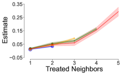
(a)

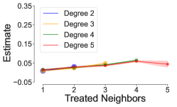
(b)

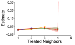
(c)

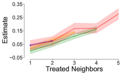
(d)

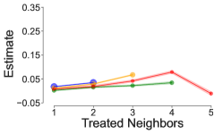
(e)

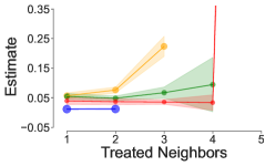
(f)

Figure 2: Spillover effects using order-$p$ GLMs

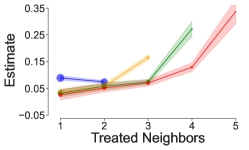
(a)

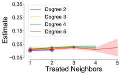
(b)

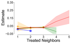
(c)

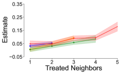
(d)

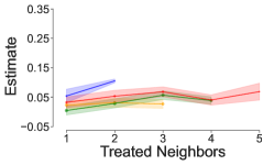
(e)

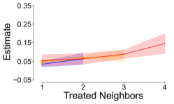
(f)

Figure 3: Spillover effects using layer-$L$ GNNs

GLM estimates vary quite substantially with the polynomial order $p$. For $p=1$, we obtain extremely large spillover effects for both treated and untreated egos. For instance, for units with degree five, whether treated or not, those with five emoji-using peers transact 0.25 times more per day than those with no such peers, an effect size three times the average outcome (0.085). With $p=2$, estimates attenuate substantially with the largest effect size being about 0.05, though this is still substantive relative to the average, with tight CIs. For $p=3$, most of the estimates are similar to $p=2$, except for a few unusual outliers. Most notably, the point estimate for $\tau=4$ and $\gamma=4$ exceeds 10 for both $d=0$ and $d=1$, which is implausibly large.

The GNN estimates for $L=1$ are similar to the $p=1$ GLM specification, yielding very large spillover effects. However, this specification only includes 1-neighborhood controls, which likely insufficiently adjusts for network confounding. With $L=2$, estimates attenuate substantially with little evidence of spillovers for $d=0$. For $d=1$, the estimates are more substantial, around 0.05, but the CIs are wide, unlike for GLMs. The results for $L=3$ tell a story closer to those of $L=2$ than $L=1$, but the estimates exhibit more extreme variation for $d=0$. For panel (f), the case $d=1,\gamma=4$ lacks estimates because the sample size after trimming is only one.

Trimming is the primary reason for the wider CIs in the figures, as seen from the dot sizes, which are proportional to sample size. For GLMs, $p=1$ estimates require significant trimming, unlike $p=2,3$. More trimming is required for GNN estimates corresponding to the ego being treated ($d=1$) and a larger number of treated neighbors $\tau$. Table III reports the sample sizes for all estimates.

The broad picture, then, is that the GNN estimates with $L>1$ yield little evidence of economically significant spillovers for non-emoji users ($d=0$, Figure 2). For emoji-users ($d=1$, Figure 3), the point estimates are more substantive but also more variable due to smaller sample sizes, resulting in wider CIs with lower bounds mostly near, if not including, zero. In either case, an additional unit increase in the number of emoji-using peers does not significantly increase the spillover effect after already having one such peer. These results are in sharp contrast to the rather implausibly large estimates for $L=1$, which do not adequately adjust for confounding. The $L=3$ estimates often require extreme trimming, resulting in poor performance in the form of more variable, or even non-existent, point estimates.

Table III: Sample sizes

		GLM, $d=0$			GLM, $d=1$			GNN, $d=0$			GNN, $d=1$
$\gamma$	$\tau$	$p=1$	$p=2$	$p=3$	$p=1$	$p=2$	$p=3$	$L=1$	$L=2$	$L=3$	$L=1$	$L=2$	$L=3$
2	1	44928	44883	44753	5010	42722	43041	44944	44846	44868	44944	1287	2860
	2	31357	43585	43647	4988	42722	43041	36955	43810	44868	36955	568	1568
3	1	26853	26823	26744	2584	25411	25635	26858	26833	26859	26858	5341	25470
	2	19014	25938	26031	2579	25411	25635	25565	26717	26758	25565	5150	10580
	3	4316	25502	25743	2474	25411	25635	7823	2453	26651	7823	4138	375
4	1	17735	17722	17644	1316	16637	16842	17742	17594	17645	17742	5470	1
	2	12515	17045	17120	1313	16637	16842	17468	17594	17642	17468	5521	1
	3	2673	16735	16922	1273	16637	16842	12556	14053	17099	12556	5373	1
	4	659	16604	16838	886	16613	16836	1431	672	60	1431	4886	1
5	1	12516	12508	12466	686	11643	11836	12511	12487	12448	12511	2398	1464
	2	8829	12000	12048	685	11643	11836	12372	12383	12448	12372	2423	1464
	3	1728	11729	11895	672	11643	11836	10859	12429	12448	10859	2422	1464
	4	413	11623	11828	557	11628	11827	3174	2176	12	3174	1923	636
	5	137	11580	11791	290	11595	11798	384	238	26	384	449	0

• $d=$ treatment, $\gamma=$ degree, $\tau=$ # treated neighbors, $p=$ order of GLM polynomial, $L=$ number of GNN layers.

The results are consistent with the findings in § 5 that $L=1$ is the worst-performing in terms of bias and $L=2$ the best. That section provides two explanations for the poor performance of $L=3$, both of which stem from rapid growth in $L$-neighborhood sizes. This is indeed an aspect of the Venmo network. The mean and 3rd quartile of the $L$-neighborhood size are respectively 4.3 and 5 for $L=1$, 27.0 and 25 for $L=2$, and 168.4 and 100 for $L=3$. For the latter, there are many units with $L$-neighborhood sizes in excess of 3000, with only one such unit for $L=2$.

Finally, the $p=2$ GLM estimates accord more with the GNN results than those with $p=1$ or $p=3$. The latter yields extreme estimates with implausible effect sizes.

7 Identification

This section provides conditions under which the estimand $\tau(t,t^{\prime})$ has a causal interpretation in the sense that it can be rewritten as a non-negatively weighted average of certain differences in potential outcomes $Y_{i}(\bm{d})-Y_{i}(\bm{d}^{\prime})$. Our identification results have some parallels with instrumental variables (IV). To obtain a causal interpretation for the Wald estimand, well-known results in the IV literature restrict heterogeneity in either the outcome (homogeneous treatment effects) or selection (monotonicity) stage (Imbens and Angrist, 1994; Vytlacil, 2002). The challenge in our setting is not necessarily heterogeneity but rather complex interference in both stages, and we obtain a causal interpretation by similarly restricting one or the other. Estimation and inference are robust to the restrictions in the same way that the linear IV estimator is consistent for the Wald estimand irrespective of restrictions on heterogeneity.

Our main identification result below bounds the discrepancy between $\tau(t,t^{\prime})$ and a causal quantity. In the absence of any restrictions on interference, the quality of the bound depends on the exposure mapping, and for typical mappings used in the literature, the bound is large. However, we show the bound is zero if treatments are conditionally independent given $(\bm{X},\bm{A})$.

A sufficient condition for conditional independence of treatments is

$$D_{i}=h_{n}(i,\bm{X},\bm{A},\nu_{i})\quad\text{and}\quad\{\nu_{i}\}_{i=1}^{n}\text{ are independent conditional on }(\bm{X},\bm{A}).$$ (20)

If selection into treatment is modeled as a binary game of incomplete information, as in the second part of Example 2, then the first part of (20) holds without any restrictions on social interactions. It is also common in that literature to assume that unobservables are conditionally independent (Kim, 2020; Lin and Vella, 2021; Xu, 2018), as in the second part of (20). On the other hand, if selection is modeled as a game of complete information, then (20) rules out endogenous peer effects since this would require $h_{n}(\cdot)$ to depend on $\bm{\nu}$.

Theorem 2.

Let $t,t^{\prime}\in\mathcal{T}$. Suppose that (a) there exists $K\geq 0$ such that $T_{i}$ is only a function of $i$’s $K$-neighborhood, and (b) conditional on $\bm{A}$, $T_{i}=t^{\prime}$ implies $\bm{D}_{\mathcal{N}(i,K)}=\bm{\delta}$ for some $\bm{\delta}\in\{0,1\}^{\lvert\mathcal{N}(i,K)\rvert}$. Let $\bm{d}_{-\mathcal{N}(i,K)}$ denote the subvector of $\bm{d}\in\{0,1\}^{n}$ restricted to $\mathcal{N}_{n}\backslash\mathcal{N}(i,K)$. Under Assumption 1,

$$\tau(t,t^{\prime})=\frac{1}{m_{n}}\sum_{i\in\mathcal{M}_{n}}\bigg{(}\sum_{\bm{d}\in\{0,1\}^{n}}{\bf E}\big{[}Y_{i}\big{(}(\bm{d}_{\mathcal{N}(i,K)},\bm{d}_{-\mathcal{N}(i,K)})\big{)}-Y_{i}\big{(}(\bm{\delta},\bm{d}_{-\mathcal{N}(i,K)})\big{)}\mid\bm{X},\bm{A}\big{]}\,\\ \times{\bf P}(\bm{D}=\bm{d}\mid T_{i}=t,\bm{X},\bm{A})\bigg{)}+\mathcal{R}_{n}.$$ (21)

for some the bias term $\mathcal{R}_{n}$. If (6) holds, then $\lvert\mathcal{R}_{n}\rvert\leq\gamma_{n}(K)$ a.s. If $\{D_{i}\}_{i=1}^{n}$ is independently distributed conditional on $(\bm{X},\bm{A})$, then $\mathcal{R}_{n}=0$.

Proof. See § SA.4.  

With $\mathcal{R}_{n}=0$, the right-hand side of (21) is a non-negatively weighted average of unit-level treatment/spillover effects that compare outcomes under different $K$-neighborhood treatment configurations. Assumption (a) is satisfied for most exposure mappings of interest, including those satisfying Assumption 3 for $K=1$. Assumption (b) concerns the choice of exposure mapping, and the following example illustrates the main cases of interest.

Example 11.

Suppose $\mathcal{R}_{n}=0$. First consider the exposure mapping $T_{i}=D_{i}$ with $t=1$ and $t^{\prime}=0$. Then $K=0$, and $T_{i}=t^{\prime}$ implies $i$’s 0-neighborhood (only itself) is untreated. Here (21) is a weighted average of the unit-level treatment effect $Y_{i}((1,\bm{d}_{-i}))-Y_{i}((0,\bm{d}_{-i}))$.

Second, consider the exposure mapping in Example 3 with $t=(d,1)$ and $t^{\prime}=(d,0)$ for any $d\in\{0,1\}$. Then $K=1$, and $T_{i}=t^{\prime}$ implies $i$’s 1-neighborhood, excluding itself, is untreated. Here (21) takes a weighted average of unit-level spillover effects of having one versus no treated neighbors for units with treatment $d$ and degree in $\bm{\Gamma}$.

Third, consider Example 4 with $t=(d,\tau)$ and $t^{\prime}=(d,0)$ with $\tau\in[0,\gamma]$. Then $K=1$, and $T_{i}=t^{\prime}$ implies $i$’s 1-neighborhood, excluding itself, is untreated. Here (21) is a weighted average of unit-level spillover effects of having $\tau$ versus no treated neighbors for units with treatment $d$ and degree $\gamma$.

If treatments are not conditionally independent, Theorem 2 provides a sort of “approximate” causal interpretation for $\tau(t,t^{\prime})$ for exposure mappings with large $K$. The approximation error $\mathcal{R}_{n}$ shrinks with the neighborhood radius $K$ under Assumption 2. This induces a bias-variance trade-off since exposure mappings with larger $K$ reduce bias but increase the variance of $\hat{\tau}(t,t^{\prime})$ due to lesser overlap. The following example provides a class of exposure mappings for which values of $K>1$ are of interest, though this class does not generally satisfy Assumption 3, which is required by our results in § 8.

Example 12.

Let $(\bm{d},\bm{a}),(\bm{d}^{\prime},\bm{a})$ lie in the support of $(\bm{D}_{\mathcal{N}(i,K)},\bm{A}_{\mathcal{N}(i,K)})$, which we assume does not depend on $i$ (see Proposition SA.2.1 for sufficient conditions). Define

$$T_{i}=\left\{\begin{array}[]{ll}1&\text{if }(\bm{D}_{\mathcal{N}(i,K)},\bm{A}_{\mathcal{N}(i,K)})\cong(\bm{d},\bm{a})\\ 0&\text{if }(\bm{D}_{\mathcal{N}(i,K)},\bm{A}_{\mathcal{N}(i,K)})\cong(\bm{d}^{\prime},\bm{a})\end{array}\right.$$

and $\mathcal{M}_{n}=\{i\in\mathcal{N}_{n}\colon\bm{A}_{\mathcal{N}(i,K)}\cong\bm{a}\}$, where $\cong$ denotes graph isomorphism. Then $\tau(1,0)$ measures the effect of changing a unit’s $K$-neighborhood treatment configuration from $\bm{d}^{\prime}$ to $\bm{d}$ for units whose $K$-neighborhood subgraph is $\bm{a}$. This is essentially the estimand studied in §4.3 of Auerbach and Tabord-Meehan (2023).

Several papers noted in § 1.4 (e.g. Lin and Vella, 2021) study models with neighborhood interference in the outcome stage and a parametric model of treatment selection with social interactions. Our next result provides a nonparametric identification result for this setting. Thus, unlike the previous result, it restricts interference in the outcome stage but not the selection stage. The outcome-stage restriction modestly weakens neighborhood interference to no interference beyond $K$-neighbors without requiring “correct specification” of $T_{i}$ in the sense of (1). While this rules out endogenous peer effects in outcomes, it imposes no restrictions on the dependence structure of $\bm{D}$ and hence allows for endogenous peer effects in treatment selection, whether modeled as a game of complete or incomplete information.

Theorem 3.

Let $t,t^{\prime}\in\mathcal{T}$. Suppose that (a) there exist $c,K\geq 0$ such that (6) holds with $\sup_{n}\gamma_{n}(s)\leq c\,\bm{1}\{s\leq K\}$, so that we may write $Y_{i}(\bm{d})=\tilde{Y}_{i}(\bm{d}_{\mathcal{N}(i,K)})$, and (b) conditional on $\bm{A}$, $T_{i}=t^{\prime}$ implies $\bm{D}_{\mathcal{N}(i,K)}=\bm{\delta}$ for some $\bm{\delta}\in\{0,1\}^{\lvert\mathcal{N}(i,K)\rvert}$. Under Assumption 1,

$$\tau(t,t^{\prime})=\frac{1}{m_{n}}\sum_{i\in\mathcal{M}_{n}}\bigg{(}\sum_{\bm{d}\in\{0,1\}^{\lvert\mathcal{N}(i,K)\rvert}}{\bf E}\big{[}\tilde{Y}_{i}(\bm{d})-\tilde{Y}_{i}(\bm{\delta})\mid\bm{X},\bm{A}\big{]}\,\\ \times{\bf P}(\bm{D}_{\mathcal{N}(i,K)}=\bm{d}\mid T_{i}=t,\bm{X},\bm{A})\bigg{)}.$$ (22)

Proof. See § SA.4.  

Assumption (a) imposes no interference beyond the $K$-neighborhood. Assumption (b) is the same as that of Theorem 2.

Example 13.

Consider the exposure mappings in Example 3 with $t^{\prime}=(d,0)$ and Example 4 with $t^{\prime}=(d,0)$ for any $d\in\{0,1\}$ and $\gamma\in\mathbb{N}$. In both cases, $K=1$, and $T_{i}=t^{\prime}$ implies $D_{i}=d$ and $i$’s neighbors are untreated, so $\bm{\delta}=(d,0,\dots,0)$. The estimand (22) thus compares units with $\bm{D}_{\mathcal{N}(i,1)}=\bm{d}$ to those with $\bm{D}_{\mathcal{N}(i,1)}=(d,0,\dots,0)$, taking a weighted average over values of $\bm{d}$. For example, if $T_{i}=t$ implies $\bm{D}_{\mathcal{N}(i,1)}=(1-d,0,\dots,0)$ (e.g. Example 3 with $t=(1-d,0)$), then (22) measures the direct effect of the treatment for units with no treated neighbors.

8 Asymptotic Theory

We study the asymptotic properties of $\hat{\tau}(t,t^{\prime})$ and $\hat{\sigma}^{2}$ under a sequence of models sending $n\rightarrow\infty$. Along this sequence, the functions $(f_{n},g_{n},h_{n})$ may obviously vary, as may the distribution of the model primitives $(\bm{A},\bm{X},\bm{\varepsilon},\bm{\nu})$, subject to the conditions imposed below. Define

$$\varphi_{t,t^{\prime}}(i)=\frac{\bm{1}\{T_{i}=t\}(Y_{i}-\mu_{t}(i,\bm{X},\bm{A}))}{p_{t}(i,\bm{X},\bm{A})}+\mu_{t}(i,\bm{X},\bm{A})\\ -\frac{\bm{1}\{T_{i}=t^{\prime}\}(Y_{i}-\mu_{t^{\prime}}(i,\bm{X},\bm{A}))}{p_{t^{\prime}}(i,\bm{X},\bm{A})}-\mu_{t^{\prime}}(i,\bm{X},\bm{A})-\tau(t,t^{\prime}),$$

whose average over $i\in\mathcal{M}_{n}$ is the doubly robust moment condition, and let

$$\sigma_{n}^{2}=\text{Var}\left(\frac{1}{\sqrt{m_{n}}}\sum_{i\in\mathcal{M}_{n}}\varphi_{t,t^{\prime}}(i)\,\bigg{|}\,\bm{X},\bm{A}\right).$$

Assumption 6 (Moments).

(a) There exists $M<\infty$ and $p>4$ such that for any $n\in\mathbb{N}$, $i\in\mathcal{N}_{n}$, and $\bm{d}\in\{0,1\}^{n}$, ${\bf E}[\lvert Y_{i}(\bm{d})\rvert^{p}\mid\bm{X},\bm{A}]<M$ a.s. (b) There exists $[\underline{\pi},\overline{\pi}]\subset(0,1)$ such that $\hat{p}_{t}(i,\bm{X},\bm{A}),p_{t}(i,\bm{X},\bm{A})\in[\underline{\pi},\overline{\pi}]$ and $m_{n}/n\geq\underline{\pi}$ a.s. for all $n\in\mathbb{N}$, $i\in\mathcal{M}_{n}$, $t\in\mathcal{T}$. (c) $\liminf_{n\rightarrow\infty}\sigma_{n}^{2}>0$ a.s.

Part (a) is a standard moment condition, and (b) requires sufficient overlap. Under Assumption 3, this is easy to satisfy if $\bm{\Gamma}$ is a bounded set. Part (b) also imposes overlap on the propensity score estimator, which is common in the double machine learning literature (e.g. Chernozhukov et al., 2018; Farrell, 2018; Farrell et al., 2021). It also requires that $\mathcal{M}_{n}$ is a nontrivial subset of $\mathcal{N}_{n}$. Part (c) is a standard non-degeneracy condition.

Assumption 7 (GNN Rates).

For any $t\in\mathcal{T}$, both $m_{n}^{-1}\sum_{i\in\mathcal{M}_{n}}(\hat{p}_{t}(i,\bm{X},\bm{A})-p_{t}(i,\bm{X},\bm{A}))^{2}$ and $m_{n}^{-1}\sum_{i\in\mathcal{M}_{n}}(\hat{\mu}_{t}(i,\bm{X},\bm{A})-\mu_{t}(i,\bm{X},\bm{A}))^{2}$ are $o_{p}(1)$, their product is $o_{p}(n^{-1})$, and $m_{n}^{-1}\sum_{i\in\mathcal{M}_{n}}(\hat{\mu}_{t}(i,\bm{X},\bm{A})-\mu_{t}(i,\bm{X},\bm{A}))(1-\bm{1}\{T_{i}=t\}p_{t}(i,\bm{X},\bm{A})^{-1})=o_{p}(n^{-1/2})$.

These are standard conditions (e.g. Assumption 3 of Farrell, 2018) but often challenging to verify for machine learners. Farrell et al. (2021) provide sufficient conditions for MLPs under i.i.d. data. We discuss the prospects of verification in § 4 and § SA.1.

The next assumption is used to show that $\{\varphi_{t,t^{\prime}}(i)\}_{i=1}^{n}$ is $\psi$-dependent (see Definition SA.5.1, which is due to Kojevnikov et al., 2021) in order to apply a central limit theorem. It imposes restrictions on the rate at which a certain dependence measure decays relative to the growth rate of network neighborhoods. Define

$$\mathcal{N}^{\partial}(i,s)=\{j\in\mathcal{N}_{n}\colon\ell(i,j)=s\}\quad\text{and}\quad\delta_{n}^{\partial}(s;k)=\frac{1}{n}\sum_{i=1}^{n}\lvert\mathcal{N}^{\partial}(i,s)\rvert^{k},$$

respectively $i$’s $s$-neighborhood boundary and the $k$th moment of the $s$-neighborhood boundary size. Let

$$\Delta_{n}(s,m;k)=\frac{1}{n}\sum_{i=1}^{n}\max_{j\in\mathcal{N}^{\partial}(i,s)}\lvert\mathcal{N}(i,m)\backslash\mathcal{N}(j,s-1)\rvert^{k},$$

$$c_{n}(s,m;k)=\inf_{\alpha>1}\Delta_{n}(s,m;k\alpha)^{1/\alpha}\delta_{n}^{\partial}(s;\alpha/(\alpha-1))^{1-1/\alpha},\quad\text{and}$$

$$\psi_{n}(s)=\max_{i\in\mathcal{N}_{n}}\left(\gamma_{n}(s/4)+\eta_{n}(s/4)\big{(}1+n(i,1)+\Lambda_{n}(i,s/4)\,n(i,s/4)\big{)}\right),$$ (23)

where $\Lambda_{n}(i,s/4)$ is a constant defined in the next assumption. The second quantity measures network density. The third bounds the covariance between $\varphi_{t,t^{\prime}}(i)$ and $\varphi_{t,t^{\prime}}(j)$ when $\ell_{\bm{A}}(i,j)\leq s$. Lastly, define

$$G_{n}(i,\bm{d}_{\mathcal{N}(i,s)})={\bf E}[g_{n(i,s)}(i,\bm{d}_{\mathcal{N}(i,s)},\bm{X}_{\mathcal{N}(i,s)},\bm{A}_{\mathcal{N}(i,s)},\bm{\varepsilon}_{\mathcal{N}(i,s)})\mid\bm{X},\bm{A}].$$

Assumption 8 (Weak Dependence).

(a) $\{(\varepsilon_{i},\nu_{i})\}_{i=1}^{n}$ is independently distributed conditional on $(\bm{X},\bm{A})$. (b) For any $n\in\mathbb{N}$, $i\in\mathcal{N}_{n}$, $s\geq 0$, and $\bm{d},\bm{d}^{\prime}\in\{0,1\}^{n}$,

$$\lvert G_{n}(i,\bm{d}_{\mathcal{N}(i,s)})-G_{n}(i,\bm{d}_{\mathcal{N}(i,s)}^{\prime})\rvert\leq\Lambda_{n}(i,s)\sum_{j\in\mathcal{N}(i,s)}\lvert d_{j}-d_{j}^{\prime}\rvert\quad\text{a.s.}$$

for some constant $\Lambda_{n}(i,s)$ that may depend on $(\bm{X},\bm{A})$. (c) $\sup_{n\in\mathbb{N}}\max_{s\geq 1}\psi_{n}(s)<\infty$ a.s. (d) For $p$ in Assumption 6(a), some positive sequence $v_{n}\rightarrow\infty$ and any $k\in\{1,2\}$,

$$\frac{1}{n^{k/2}}\sum_{s=0}^{\infty}c_{n}(s,v_{n};k)\psi_{n}(s)^{1-(2+k)/p}\rightarrow 0,\quad n^{3/2}\psi_{n}(v_{n})^{1-1/p}\rightarrow 0,\quad\text{and}\\ \limsup_{n\rightarrow\infty}\sum_{s=0}^{\infty}\delta_{n}^{\partial}(s;2)^{1/2}\gamma_{n}(s/2)^{1-2/p}<\infty\quad\text{a.s.}$$ (24)

Parts (a) and (b) are used to establish that $\{\varphi_{t,t^{\prime}}(i)\}_{i=1}^{n}$ is $\psi$-dependent; (b) is a smoothness condition, while (a) restricts dependence in unobservables. These conditions, particularly (a), are likely stronger than necessary, but they facilitate the task of verifying $\psi$-dependence given that treatments are complex functions of unobservables and $Y_{i}$ and $T_{i}$ are complex functions of treatments. Independence of unobservables can be potentially relaxed given some additional structure, as in Proposition 2.5 of Kojevnikov et al. (2021). The simulation study in § 5 provides evidence that our methods can perform well when unobservables exhibit network dependence.

Perhaps the most substantive requirement is (d), which regulates the asymptotic behavior of three quantities in (24). The first two correspond to Condition ND of Kojevnikov et al. (2021), which they use to establish a CLT. The third is similar and is used to asymptotically linearize the doubly robust estimator under network dependence. We illustrate how to verify (24) in § SA.3.1.

Part (d) implies that $\psi_{n}(s)\rightarrow 0$ as $s\rightarrow\infty$ essentially uniformly in $n$. Verifying this requires a uniform bound on $\Lambda_{n}(i,s)$ due to its appearance in $\psi_{n}(s)$. Such a bound exists in the case of Example 1, which is easily seen by taking the derivative of the reduced form with respect to $\bm{D}$. In Example 2, a uniform bound also exists because outcomes are binary.

Theorem 4.

Under Assumptions 1–3 and 6–8,

$$\sigma_{n}^{-1/2}\sqrt{m_{n}}\big{(}\hat{\tau}(t,t^{\prime})-\tau(t,t^{\prime})\big{)}\stackrel{{\scriptstyle d}}{{\longrightarrow}}\mathcal{N}(0,1).$$

Proof. See § SA.4.  

Our last result characterizes the asymptotic properties of $\hat{\sigma}^{2}$. Similar to the design-based setting of Leung (2022a), it is not guaranteed to be consistent due to conditioning on $(\bm{X},\bm{A})$. However, as in that setting, we can make the case that it is typically asymptotically conservative. Define

$$\mathcal{J}_{n}(s,m)=\left\{(i,j,k,l)\in\mathcal{N}_{n}^{4}\colon k\in\mathcal{N}(i,m),l\in\mathcal{N}(j,m),\ell_{\bm{A}}(i,j)=s\right\}.$$

Assumption 9 (HAC).

(a) For some $M>0$ and all $n\in\mathbb{N}$, $i\in\mathcal{N}_{n}$, and $t\in\mathcal{T}$, $\lvert\max\{Y_{i},\hat{\mu}_{t}(i,\bm{X},\bm{A})\}\rvert<M$ a.s. (b) $m_{n}^{-1}\sum_{i\in\mathcal{M}_{n}}(\hat{p}_{t}(i,\bm{X},\bm{A})-p_{t}(i,\bm{X},\bm{A}))^{2}$ and $m_{n}^{-1}\sum_{i\in\mathcal{M}_{n}}(\hat{\mu}_{t}(i,\bm{X},\bm{A})-\mu_{t}(i,\bm{X},\bm{A}))^{2}$ are $o_{p}(n^{-1/2})$. (c) For some $\epsilon\in(0,1)$ and $b_{n}\rightarrow\infty$, $\lim_{n\rightarrow\infty}n^{-1}\sum_{s=0}^{\infty}c_{n}(s,b_{n};2)\psi_{n}(s)^{1-\epsilon}=0$ a.s. (d) $n^{-1}\sum_{i=1}^{n}n(i,b_{n})=o_{p}(\sqrt{n})$. (e) $n^{-1}\sum_{i=1}^{n}n(i,b_{n})^{2}=O_{p}(\sqrt{n})$. (f) $\sum_{s=0}^{n}\lvert\mathcal{J}_{n}(s,b_{n})\rvert\psi_{n}(s)=o(n^{2})$.

Part (a) strengthens Assumption 6(a) to uniformly bounded outcomes. Part (b) strengthens Assumption 7(b) but only mildly so since we nonparametrically estimate both nuisance functions. Since it does not require uniform convergence, it is more readily verifiable for machine learning estimators. Part (c) is Assumption 4.1(iii) of Kojevnikov et al. (2021), and parts (d)–(f) correspond to Assumptions 7(b)–(d) of Leung (2022a). The latter are used to characterize the bias of the variance estimator. We discuss verification of (c)–(f) in § SA.3.2; the derivations there show that (f) is closely related to (c).

Theorem 5.

Define $\tilde{\varphi}_{t,t^{\prime}}(i)$ by replacing $\tau(t,t^{\prime})$ in the definition of $\varphi_{t,t^{\prime}}(i)$ with $\tau_{i}(t,t^{\prime})={\bf E}[Y_{i}\mid T_{i}=t,\bm{X},\bm{A}]-{\bf E}[Y_{i}\mid T_{i}=t^{\prime},\bm{X},\bm{A}]$. Let

$$\hat{\sigma}^{2}_{*}=\frac{1}{m_{n}}\sum_{i\in\mathcal{M}_{n}}\sum_{j\in\mathcal{M}_{n}}\tilde{\varphi}_{t,t^{\prime}}(i)\tilde{\varphi}_{t,t^{\prime}}(j)\mathbf{1}\{\ell_{\bm{A}}(i,j)\leq b_{n}\}\quad\text{and}$$

$$R_{n}=\frac{1}{m_{n}}\sum_{i\in\mathcal{M}_{n}}\sum_{j\in\mathcal{M}_{n}}(\tau_{i}(t,t^{\prime})-\tau(t,t^{\prime}))(\tau_{j}(t,t^{\prime})-\tau(t,t^{\prime}))\mathbf{1}\{\ell_{\bm{A}}(i,j)\leq b_{n}\}.$$

Under Assumption 9 and the assumptions of Theorem 4,

$$\hat{\sigma}^{2}=\hat{\sigma}^{2}_{*}+R_{n}+o_{p}(1)\quad\text{and}\quad\lvert\hat{\sigma}^{2}_{*}-\sigma_{n}^{2}\rvert\stackrel{{\scriptstyle p}}{{\longrightarrow}}0.$$

Proof. See § SA.4.  

The conclusion is similar to that of Theorem 4 of Leung (2022a), which does not allow for first-stage estimators. As in that theorem, $\hat{\sigma}^{2}$ is asymptotically biased by $R_{n}$. If we were to use a positive-semidefinite kernel function as in Leung (2019) instead of the uniform kernel $\mathbf{1}\{\ell_{\bm{A}}(i,j)\leq b_{n}\}$, then $R_{n}\geq 0$ a.s., in which case Theorem 5 would imply that $\hat{\sigma}^{2}$ is asymptotically conservative. However, in simulations in past work, we found that the uniform kernel better controls size than sloped alternatives, which is why we use it even though it does not guarantee positive semidefiniteness.

Although we can no longer guarantee non-negativity of $R_{n}$ for any given $n$, we observe that $R_{n}$ is a HAC estimate of the variance of the unit-level contrasts $\tau_{i}(t,t^{\prime})$. It should therefore well approximate $\text{Var}(m_{n}^{-1/2}\sum_{i\in\mathcal{M}_{n}}\tau_{i}(t,t^{\prime}))\geq 0$ in which case $\hat{\sigma}^{2}$ would be asymptotically conservative. This can be formalized under additional weak dependence conditions on the superpopulation as in §A of Leung (2022b).

9 Conclusion

Existing work on network interference under unconfoundedness assumes that it suffices to control for a known, low-dimensional function of the network and covariates. We propose to use GNNs to effectively learn this function and provide a behavioral model under which it is low-dimensional and estimable with shallow GNNs. More formally, we provide conditions under which the propensity score and outcome regression, which ordinarily may depend on the entirety of the network, can be approximated by functions of the ego’s $L$-neighborhood network for relatively small $L$. This is analogous to approximate sparsity conditions in the lasso literature, which posit that a high-dimensional regression function is well-approximated by a function of a relatively small number of covariates. Our key assumption is approximate neighborhood interference. Leung (2022a) studies its implications for asymptotic inference in randomized control trials, while we highlight its utility for estimation with high-dimensional network controls in observational settings.

Our large-sample results rely on high-level conditions on the rate of convergence of the GNN estimators. Primitive sufficient conditions are beyond the scope of the current literature, but we provide two potentially useful results on this front. The first provides primitive conditions for a network analog of approximate sparsity, and the second reframes and combines existing work in the GNN literature to characterize the nonparametric function class that GNNs approximate for any given choice of depth.

Finally, we study commonly used estimands defined by exposure mappings and provide conditions under which they constitute non-negatively weighted averages of unit-level causal effects. The conditions restrict interference in either the outcome or treatment selection stage. This is similar to how the Wald estimand in the instrumental variables literature obtains a causal interpretation under restrictions on heterogeneity in either stage.

SA.1 Additional Results on GNNs

Verifying Assumption 7 appears to be beyond the scope of existing results for GNNs. Farrell et al. (2021) provide a bound for MLPs, which, were it applicable to our setting, would be of the form

$$\frac{1}{n}\sum_{i=1}^{n}(\hat{p}_{t}(i,\bm{X},\bm{A})-p_{t}(i,\bm{X},\bm{A}))^{2}\leq C\left(\frac{WL\log R}{n}\log n+\frac{\log\log n+\gamma}{n}+\epsilon^{2}\right)$$ (SA.1.1)

with probability at least $1-e^{-\gamma}$. Here $W$ is the number of parameters, $C$ is a constant that does not depend on $n$, $R$ depends on the architecture through the number of hidden neurons, and $\epsilon$ is the function approximation error, a measure of the ability of the neural network to approximate any function in a desired class. Establishing a corresponding result for GNNs requires an analog of Lemma 6 of Farrell et al. (2021), which is a bound on the pseudo-dimension of the GNN class, and concentration inequalities for $\psi$-dependent data. Jegelka (2022) surveys the few available complexity and generalization bounds for GNNs. These are not sufficiently general for our setup and only apply to settings where we observe a large sample of independent networks.

Additionally, usage of a bound of the form (SA.1.1) for verifying Assumption 7 requires knowledge of how $\epsilon$ varies with key aspects of the architecture, such as $W,R,L,n$. As a first step toward obtaining such a result, it is necessary to characterize the function class that GNNs can approximate (i.e. the class for which $\epsilon=0$). Our next result, which draws heavily from existing results in the GNN literature, shows that an additional shape restriction on the function class beyond invariance (Assumption 4) is required.

SA.1.1 WL Function Class

MLPs can approximate any measurable function (Hornik et al., 1989), so a natural question is whether GNNs can approximate any measurable, invariant function of graph-structured inputs. In other words, is it enough to impose Assumption 4 (and regularity conditions), or do we need stronger restrictions on the function class? It turns out stronger restrictions are required for reasons related to the graph isomorphism problem. We next motivate the need for such restrictions and then state our function approximation result.

Chen et al. (2019) show that, for a function class such as GNNs to approximate any invariant function, some element of the class must be able to separate any pair of non-isomorphic graphs. By “separate,” we mean that for any non-isomorphic labeled graphs $(\bm{X},\bm{A}),(\bm{X}^{\prime},\bm{A}^{\prime})$, the function $f$ satisfies $f(\bm{X},\bm{A})\neq f(\bm{X}^{\prime},\bm{A}^{\prime})$. Hence, a function with separating power of this sort solves the graph isomorphism problem, a problem for which no known polynomial-time solution exists (Kobler et al., 2012; Morris et al., 2021). Since GNNs can be computed in polynomial time, this suggests that approximating any invariant function is too demanding of a requirement.

To define the subclass of invariant functions that GNNs can approximate, we need to take a detour and discuss graph isomorphism tests. The subclass will be defined by a weaker graph separation criterion than solving the graph isomorphism problem, in particular one defined by the Weisfeiler-Leman (WL) test. This is a (generally imperfect) test for graph isomorphism on which almost all practical graph isomorphism solvers are based (Morris et al., 2021).

Given a labeled graph $(\bm{X},\bm{A})$, the WL test outputs a graph coloring (a vector of labels for each unit) according to the following recursive procedure, whose definition follows Maron et al. (2019). At each iteration $t>0$, each unit $i$ is assigned a color $C_{t}(i)$ from some set $\Sigma$ (e.g. the natural numbers) according to

$$C_{t}(i)=\Phi\left(C_{t-1}(i),\{C_{t-1}(j)\colon A_{ij}=1\}\right),$$ (SA.1.2)

where $\Phi(\cdot)$ is a bijective function that takes as input a color and a multiset of neighbors’ colors. Intuitively, at each iteration, two units are assigned different colors if they differ in the number of identically colored neighbors, so that at iteration $t$, colors capture some information about a unit’s $(t-1)$-neighborhood. Colors are initialized at $t=0$ using a deterministic rule that assigns each $i$ to the same color $C_{0}(i)\in\Sigma$ if and only if they have the same covariates $X_{i}$. At each iteration, the number of assigned colors increases, and the algorithm converges when the coloring is the same in two adjacent iterations. This takes at most $n-1$ iterations since there cannot be more than $n$ distinctly assigned colors.

To test whether two labeled graphs are isomorphic, the procedure is run in parallel on both graphs until some number of iterations, typically until convergence. At this point, if there exists a color such that the number of units assigned that color differs in the two graphs, then the graphs are considered non-isomorphic. This procedure correctly separates non-isomorphic graphs, but it is underpowered since there exist non-isomorphic graphs considered isomorphic by the WL test (Morris et al., 2021). Also, because the number of colors increases each iteration, the test is more powerful when run longer.

Morris et al. (2019) and Xu et al. (2018) note the similarity between the GNN architecture (12) and WL test (SA.1.2). The former may be viewed as a continuous approximation of the latter, replacing the hash function $\Phi(\cdot)$ with a learnable aggregator $\Phi_{1l}(\cdot)$. They formally show that any GNN has at most the graph separation power of the WL test and furthermore that there exist architectures as powerful.

Returning to the original problem, we now define the class of functions approximated by GNNs in terms of the WL test. Let $H$ denote the support of $(\bm{X},\bm{A})$.

Definition 2.

For any set of functions $\mathcal{F}$ with domain $H$, let $\rho(\mathcal{F})$ be the subset of $H^{2}$ such that

$$(h,h^{\prime})\in\rho(\mathcal{F})\quad\text{if and only if}\quad f(h)=f(h^{\prime})\quad\text{for all}\quad f\in\mathcal{F}.$$

For any two sets of functions $\mathcal{E},\mathcal{F}$ with domain $H$, we say that $\mathcal{E}$ is at most as separating as $\mathcal{F}$ if $\rho(\mathcal{F})\subseteq\rho(\mathcal{E})$.

This is essentially Definition 2 of Azizian and Lelarge (2021). Intuitively, if $\mathcal{E}$ is at most as separating as $\mathcal{F}$, the latter is more complex in the sense that some function in $\mathcal{F}$ can separate weakly more elements of $H$ than any function in $\mathcal{E}$.

Let $f_{\text{WL},L}$ denote the function of $(\bm{X},\bm{A})$ with range $\Sigma^{n}$ that outputs the vector of node colorings from the WL test run for $L$ iterations. Let $\mathcal{C}(H)$ be the set of continuous functions with domain $H$. For any $L\in\mathbb{N}$, define the WL function class

$$\mathcal{F}_{\text{WL}}(L)=\{f^{*}\in\mathcal{C}(H)\colon\rho(\{f_{\text{WL},L}\})\subseteq\rho(f^{*})\}.$$

This is the set of continuous functions of $(\bm{X},\bm{A})$ that are at most as separating as the WL test with $L$ iterations.

The next result says that $p_{t}(\cdot)$ and $\mu_{t}(\cdot)$ can be approximated by $L$-layer GNNs under the shape restriction that they are elements of the WL function class. This is a stronger shape restriction than Assumption 4 because, as previously discussed, functions satisfying invariance can also solve the graph isomorphism problem. The WL test does not, but by construction, its outputs are invariant, so $\mathcal{F}_{\text{WL}}(L)$ is a subset of the set of all invariant functions.

Consider the GNN architecture in Example 6 with $\phi_{0l}(\cdot),\phi_{1l}(\cdot)$ being MLPs. For technical reasons, we augment the architecture with an additional MLP layer $L+1$ at the output stage with $n$ neurons and the $i$th neuron given by $h_{i}^{(L+1)}=\phi_{L+1}(h_{i}^{(L)},\{h_{j}^{(L)}\colon j\in\mathcal{N}_{n}\})$. Interpret this as the actual output layer, and let $L$ only enumerate the number of hidden layers (i.e. not counting the input $h_{i}^{(0)}$ and output $h_{i}^{(L+1)}$ layers). Let $\mathcal{F}_{\text{GNN}*}(L)$ denote the set of such GNNs with $L$ layers, ranging over the parameter space of the MLPs, including their widths and depths.

Theorem SA.1.1.

Fix $n,L\in\mathbb{N}$. Suppose that each $X_{i}$ has the same common, finite support. For any $f^{*}\in\mathcal{F}_{\text{WL}}(L)$, there exists a sequence of GNNs $\{f_{k}\}_{k\in\mathbb{N}}\subseteq\mathcal{F}_{\text{GNN}*}(L)$ such that

$$\sup_{(\bm{X},\bm{A})\in H}\lvert f_{k}(1,\bm{X},\bm{A})-f^{*}(1,\bm{X},\bm{A})\rvert\stackrel{{\scriptstyle k\rightarrow\infty}}{{\longrightarrow}}0.$$ (SA.1.3)

In other words, any function in the class $\mathcal{F}_{\text{WL}}(L)$ can be approximated by $L$-layer GNNs in $\mathcal{F}_{\text{GNN}*}(L)$. The result is a consequence of a Stone-Weierstrauss theorem due to Azizian and Lelarge (2021) and a version of the Morris et al. (2019) and Xu et al. (2018) result on the equivalent separation power of GNNs and the WL test. The proof is given below.

The result is essentially Theorem 4 of Azizian and Lelarge (2021) but with the distinction that they use $\mathbin{\scalebox{1.5}{$\cup$}}_{L}\mathcal{F}_{\text{GNN}*}(L)$ in place of $\mathcal{F}_{\text{GNN}*}(L)$ and $\{f_{\text{WL},\infty}\}$ in place of $\{f_{\text{WL},L}\}$. That is, their theorem states that the set of GNNs ranging over all possible numbers of layers can approximate any continuous function at most as separating as the WL test run until convergence.

Theorem SA.1.1 states their result for fixed $L$, and the proof is straightforward from prior results. However, our framing clarifies one of the roles of depth, namely that it determines the strength of the shape restriction implicitly imposed on the function being approximated by GNNs. In particular, because the WL test is more powerful when $L$ is larger, meaning when run for more iterations, Theorem SA.1.1 implies that deeper GNNs can approximate weakly richer function classes, or equivalently, impose weaker shape restrictions. See the next subsection for further discussion.

Proof of Theorem SA.1.1. Lemma 35 of Azizian and Lelarge (2021) (in particular the result for $MGNN_{E}$) shows that there exists a sequence of GNNs $\{f_{k}\}_{k\in\mathbb{N}}\subseteq\mathbin{\scalebox{1.5}{$\cup$}}_{L}\mathcal{F}_{\text{GNN}*}(L)$ such that (SA.1.3) holds for any $f^{*}$ in the class

$$\{f^{*}\in\mathcal{C}(H)\colon\rho(\mathbin{\scalebox{1.5}{$\cup$}}_{L}\mathcal{F}_{\text{GNN}*}(L))\subseteq\rho(f^{*})\}.$$

In contrast, we would like to establish that, for any fixed $L$, there exists a sequence of GNNs $\{f_{k}\}_{k\in\mathbb{N}}\subseteq\mathcal{F}_{\text{GNN}*}(L)$ such that (SA.1.3) holds for any $f^{*}$ in the class

$$\{f^{*}\in\mathcal{C}(H)\colon\rho(\mathcal{F}_{\text{GNN}*}(L))\subseteq\rho(f^{*})\},$$ (SA.1.4)

meaning that an $L$-layer GNN can arbitrarily approximate any continuous function at most as separating as an $L$-layer GNN. The argument in the proof of Lemma 35 actually applies to (SA.1.4) after some minor changes to notation. The first part of the proof (“We now move to the equivariant case…”) up to verifying their (26) carries over by redefining the $MGNN_{E}$ class as having a fixed depth $L$. To show (26), Azizian and Lelarge (2021) begin with a GNN $f$ with $L$ layers (their notation uses $T$ in place of $L$) and add an additional MLP layer that implements (26). Here we use the additional MLP layer added to the output of our architecture (see the paragraph prior to the statement of Theorem SA.1.1). In particular, for any $f\in\mathcal{F}_{\text{GNN}*}(L)$, consider the mapping

$$(\bm{X},\bm{A})\mapsto\left(\sum_{i=1}^{n}f(i,\bm{X},\bm{A}),\dots,\sum_{i=1}^{n}f(i,\bm{X},\bm{A})\right)\in\mathbb{R}^{n}$$

(our translation of (26)) corresponds to adding a linear output layer $L+1$ that is implementable by an MLP of the form $\phi_{L+1}(h_{i}^{(L)},\{h_{j}^{(L)}\colon j\in\mathcal{N}_{n}\})$. The mapping remains an element of $\mathcal{F}_{\text{GNN}*}(L)$, which completes the argument for (SA.1.4).

By Theorems VIII.1 and VIII.4 of Grohe (2021), which use finiteness of the support of $X_{i}$, $\rho(\mathcal{F}_{\text{GNN}*}(L))=\rho(\{f_{\text{WL},L}\})$. That is, $L$-layer GNNs have the same separation power as the WL test run for $L$ iterations.  

SA.1.2 Disadvantages of Depth

The receptive field is the main consideration when selecting $L$, but Theorem SA.1.1 provides a second consideration, which is imposing a weaker implicit shape restriction. It shows that, for GNNs to approximate a target function well, the target must satisfy a shape restriction stronger than invariance, namely that it is at most as separating as the WL test with $L$ iterations. The larger the choice of $L$, the weaker the shape restriction imposed. However, there are several reasons why shallow architectures remain preferable.

Low returns to depth. A natural question is how many iterations are required for the WL test to converge for a given graph, which corresponds to the choice of $L$ for which the shape restriction is weakest. Unfortunately, the answer is not generally known, being determined by the topology of the input graph in a complex manner. However, there is a range of results bounding the number of iterations required for convergence. For instance, Kiefer and McKay (2020) construct graphs for which the WL test requires $n-1$ iterations to converge, so such graphs require $n-1$ layers to obtain the weakest shape restriction. This makes the estimation problem extremely high-dimensional, requiring substantially more layers than what is typically required for the receptive field to encompass the entirety of the network.

Fortunately, theoretical and empirical evidence suggests that such examples are more the exception than the rule and that small choices of $L$ typically already impose weak shape restrictions. Babai et al. (1980) show that, with probability approaching one as $n\rightarrow\infty$, in an $n$-unit network drawn uniformly at random from the set of all possible networks, the WL test assigns all units different colors (recall the test must converge at this point) after only two iterations (Morris et al., 2021). Thus, roughly speaking, for large networks, the weakest possible shape restriction is generically achieved with only $L=2$. Of course, having the network drawn uniformly at random is a strong assumption, so this result resides in the opposite extreme relative to the worst-case examples requiring $L=n-1$. Nonetheless, it suggests that relatively few layers may often suffice in practice. Indeed, Zopf (2022) provide empirical evidence on this point, showing that the vast majority of graphs in their dataset can be separated using the WL test after a single iteration.

Cost of depth. The end of § 5.3 discusses the oversquashing and oversmoothing phenomenon that may explain why larger choices of $L$ often produce worse performance. Zhou et al. (2021) provide a different explanation, that certain features of common architectures are responsible for variance inflation. In fact, even weaker shape restrictions than that imposed by Theorem SA.1.1 are possible using more complex “$k$-GNN” architectures, which would theoretically improve bias, but these have greater computational cost and empirically exhibit worse predictive performance and higher variance than the standard architecture (12) (Dwivedi et al., 2022). These disadvantages may partly explain the common use in practice of the standard architecture with few layers.

SA.2 Sufficient Conditions for Invariance

We state a result that provides weak sufficient conditions for Assumption 4.

Proposition SA.2.1.

Suppose for any $n\in\mathbb{N}$ and permutation $\pi$,

$$f_{n}(i,\bm{D},\bm{A})=f_{n}(\pi(i),\pi(\bm{D}),\pi(\bm{A})),\\ g_{n}(i,\bm{D},\bm{X},\bm{A},\bm{\varepsilon})=g_{n}(\pi(i),\pi(\bm{D}),\pi(\bm{X}),\pi(\bm{A}),\pi(\bm{\varepsilon})),\quad\text{and}\\ h_{n}(i,\bm{X},\bm{A},\bm{\nu})=h_{n}(\pi(i),\pi(\bm{X}),\pi(\bm{A}),\pi(\bm{\nu}))$$

a.s., and $(\bm{A},\bm{X},\bm{\varepsilon},\bm{\nu})\stackrel{{\scriptstyle d}}{{=}}(\pi(\bm{A}),\pi(\bm{X}),\pi(\bm{\varepsilon}),\pi(\bm{\nu}))$. Then Assumption 4 holds.

The first three equations impose invariance on $(f_{n},g_{n},h_{n})$. Applied to $f_{n}$, this is a restriction on the choice of exposure mapping. It is satisfied by most, if not all, such mappings used in the literature, including those satisfying Assumption 3. Applied to $(g_{n},h_{n})$, invariance only says that unit identities do not influence behavior beyond the model primitives $(\bm{A},\bm{X},\bm{\varepsilon},\bm{\nu})$. The final requirement says that these model primitives are themselves distributionally invariant, which is a weak condition since unit labels carry no intrinsic meaning in our setup.

Proof of Proposition SA.2.1. By definition, $T_{\pi(i)}=f_{n}(\pi(i),\bm{D},\bm{A})$ and

$$Y_{\pi(i)}=g(\pi(i),\bm{D},\bm{X},\bm{A},\bm{\varepsilon})=g(\pi(i),(h_{n}(j,\bm{X},\bm{A},\bm{\nu}))_{j=1}^{n},\bm{X},\bm{A},\bm{\varepsilon}).$$

By the invariance assumptions on $f_{n},g_{n},h_{n}$,

$$Y_{i}=g(i,\bm{D},\bm{X},\bm{A},\bm{\varepsilon})=g_{n}(\pi(i),\pi(\bm{D}),\pi(\bm{X}),\pi(\bm{A}),\pi(\bm{\varepsilon}))\\ =g_{n}(\pi(i),(h_{n}(\pi(j),\pi(\bm{X}),\pi(\bm{A}),\pi(\bm{\nu})))_{j=1}^{n},\pi(\bm{X}),\pi(\bm{A}),\pi(\bm{\varepsilon})),$$

and

$$T_{i}=f_{n}(\pi(i),\pi(\bm{D}),\pi(\bm{A}))=f_{n}(\pi(i),(h_{n}(\pi(j),\pi(\bm{A}),\pi(\bm{\nu})))_{j=1}^{n},\pi(\bm{X}),\pi(\bm{A})),$$

so by the distributional exchangeability assumption,

$$(Y_{i},T_{i},\bm{X},\bm{A})\stackrel{{\scriptstyle d}}{{=}}(Y_{\pi(i)},T_{\pi(i)},\pi(\bm{X}),\pi(\bm{A})).$$

It follows that

$$\mu_{t}(i,\bm{X},\bm{A}) ={\bf E}[Y_{i}\mid T_{i}=t,\bm{X},\bm{A}]$$

$$={\bf E}[Y_{\pi(i)}\mid T_{\pi(i)}=t,\pi(\bm{X}),\pi(\bm{A})]=\mu_{t}(\pi(i),\pi(\bm{X}),\pi(\bm{A}))$$

and similarly for the generalized propensity score.  

SA.3 Verifying §8 Assumptions

Leung (2022a), §A, verifies analogs of Assumptions 8(d) and 9(c) from an older working paper version of Kojevnikov et al. (2021). This section repeats the exercise for Assumptions 8(d) and 9(c) and (d). We assume throughout that $\max\{\gamma_{n}(s/2),\psi_{n}(s)\}\leq\text{exp}(-c(1-4/p)^{-1}s)$ for some $c>0$ and $p$ in Assumption 6(a). As in Leung (2022a), we say a sequence of networks exhibits polynomial neighborhood growth if

$$\sup_{n}\max_{i\in\mathcal{N}_{n}}\,\lvert\mathcal{N}_{\bm{A}}(i,s)\rvert=Cs^{d}$$

for some $C>0$, $d\geq 1$. The sequence exhibits exponential neighborhood growth if

$$\sup_{n}\max_{i\in\mathcal{N}_{n}}\,\lvert\mathcal{N}_{\bm{A}}(i,s)\rvert=Ce^{\beta s}$$

for some $C>0$ and $\beta=\log\delta(\bm{A})$ (Leung, 2022a, §A discusses this choice of $\beta$).

SA.3.1 Assumption 8(d)

For polynomial neighborhood growth, choose $v_{n}=n^{1/(\alpha d)}$ for $\alpha>2$. The second term in (24) is at most $n^{3/2}\text{exp}(-c\,n^{1/(\alpha d)})=o(1)$. The third term is at most $\sum_{s=0}^{\infty}Cs^{d}\text{exp}(-c\,s)<\infty$. The first term is $\leq n^{-1/2}\sum_{s=0}^{\infty}(Cn^{1/\alpha})(Cs^{d})\text{exp}(-c\,s)=o(1)$ for $k=1$, and for $k=2$, it is at most $n^{-1}\sum_{s=0}^{\infty}(Cn^{1/\alpha})^{2}(Cs^{d})\text{exp}(-c\,s)=o(1)$.

For exponential neighborhood growth, choose $v_{n}=\alpha\beta^{-1}\log n$, $\alpha\in(1.5\beta c^{-1},0.5)$, with $c$ from the definition of $\psi_{n}(s)$ above. Such an $\alpha$ exists only if $c>3\beta$, which requires $\psi_{n}(s)$ to decay sufficiently fast relative to neighborhood growth. The second term in (24) is then at most $n^{3/2}\text{exp}(-c\alpha\beta^{-1}\log n)=n^{1.5-c\alpha\beta^{-1}}=o(1)$. The third term is at most $\sum_{s=0}^{\infty}C\text{exp}((\beta-c)s)<\infty$. Finally, for $k=1$, the first term is at most $n^{-1/2}\sum_{s=0}^{\infty}C^{2}\text{exp}(\alpha\log n)\text{exp}((\beta-c)s)=o(1)$, and for $k=2$, it is at most $n^{-1}\sum_{s=0}^{\infty}C^{2}\text{exp}(2\alpha\log n)\text{exp}((\beta-c)s)=o(1)$.

SA.3.2 Bandwidth

We employ a mix of formal and heuristic arguments to show that the bandwidth (11) satisfies Assumption 9(c)–(f). Under polynomial neighborhood growth, as argued in §A.2 of Leung (2022a), $\mathcal{L}(\bm{A})\approx n^{1/d}$, in which case $b_{n}=\mathcal{L}(\bm{A})^{1/4}\approx n^{1/(4d)}$. Then Assumption 9(d) holds because $n^{-1}\sum_{i=1}^{n}n(i,b_{n})=Cb_{n}^{d}\approx n^{1/4}=o(\sqrt{n})$, and Assumption 9(e) holds because $n^{-1}\sum_{i=1}^{n}n(i,b_{n})^{2}=Cb_{n}^{2d}\approx n^{1/2}=O(\sqrt{n})$. Assumption 9(c) holds because, taking $\epsilon=1-4/p$,

$$n^{-1}\sum_{s=0}^{\infty}c_{n}(s,b_{n};2)\psi_{n}(s)^{1-4/p} \leq C^{3}n^{-1}\sum_{s=0}^{\infty}b_{n}^{2d}s^{d}\text{exp}(-c\,s)$$ (SA.3.1)

$$\approx n^{-1}\sqrt{n}\sum_{s=0}^{n}s^{d}\text{exp}(-c\,s)=O(n^{-1/2}).$$

Finally, Assumption 9(f) holds because

$$\frac{1}{n^{2}}\sum_{s=0}^{n}\lvert\mathcal{J}_{n}(s,b_{n})\rvert\psi_{n}(s)\leq\frac{1}{n^{2}}\sum_{s=0}^{n}\sum_{i=1}^{n}\sum_{j\colon\ell_{\bm{A}}(i,j)=s}n(i,b_{n})\,n(j,b_{n})\psi_{n}(s)\leq\eqref{r910u232gj}.$$

Under exponential neighborhood growth, as argued in §A.2 of Leung (2022a), $\mathcal{L}(\bm{A})\approx\log n/\log\delta(\bm{A})$, in which case $b_{n}\approx 0.25\log n/\log\delta(\bm{A})$. Then Assumption 9(d) holds because $n^{-1}\sum_{i=1}^{n}n(i,b_{n})=C\text{exp}(\beta b_{n})\approx n^{1/4}$, and Assumption 9(e) holds because $n^{-1}\sum_{i=1}^{n}n(i,b_{n})^{2}=C\text{exp}(2\beta b_{n})\approx\sqrt{n}$. Assumption 9(c) holds because, taking $\epsilon=1-4/p$,

$$n^{-1}\sum_{s=0}^{\infty}c_{n}(s,b_{n};2)\psi_{n}(s)^{1-4/p} \leq C^{3}n^{-1}\sum_{s=0}^{\infty}\text{exp}(\beta b_{n})\text{exp}(\beta s)\text{exp}(-c\,s)$$ (SA.3.2)

$$\approx n^{-1}\text{exp}(0.5\log n)\sum_{s=0}^{n}\text{exp}((\beta-c)s)=O(n^{-1/2}),$$

which is $o(1)$ if $c>\beta$, which is weaker than the requirement $c>3\beta$ in § SA.3.1. Finally, Assumption 9(f) holds because, if $c>\beta$, $n^{-2}\sum_{s=0}^{n}\lvert\mathcal{J}_{n}(s,b_{n})\rvert\psi_{n}(s)\leq\eqref{fg209h4}$.

SA.4 Proofs of Main Results

Proof of Theorem 2. By definition,

$$\tau(t,t^{\prime})=\frac{1}{m_{n}}\sum_{i\in\mathcal{M}_{n}}\bigg{(}\sum_{\bm{d}\in\{0,1\}^{n}}{\bf E}[Y_{i}(\bm{d})\mid\bm{X},\bm{A}]{\bf P}(\bm{D}=\bm{d}\mid T_{i}=t,\bm{X},\bm{A})\\ -\sum_{\bm{d}^{\prime}\in\{0,1\}^{n}}{\bf E}[Y_{i}(\bm{d}^{\prime})\mid\bm{X},\bm{A}]{\bf P}(\bm{D}=\bm{d}^{\prime}\mid T_{i}=t^{\prime},\bm{X},\bm{A})\bigg{)}.$$ (SA.4.1)

Using the assumption that $T_{i}=t^{\prime}$ implies $\bm{D}_{\mathcal{N}(i,K)}=\bm{\delta}$,

$$\eqref{Egen}=\frac{1}{m_{n}}\sum_{i\in\mathcal{M}_{n}}\bigg{(}\sum_{\bm{d}\in\{0,1\}^{n}}{\bf E}\big{[}Y_{i}(\bm{d})\mid\bm{X},\bm{A}\big{]}\,{\bf P}(\bm{D}=\bm{d}\mid T_{i}=t,\bm{X},\bm{A})\\ -\sum_{\bm{d}^{\prime}\in\{0,1\}^{n}}{\bf E}\big{[}Y_{i}\big{(}(\bm{\delta},\bm{d}_{-\mathcal{N}(i,K)}^{\prime})\big{)}\mid\bm{X},\bm{A}\big{]}\,{\bf P}(\bm{D}=\bm{d}^{\prime}\mid T_{i}=t^{\prime},\bm{X},\bm{A})\bigg{)}.$$

Adding and subtracting the last term with $t^{\prime}$ replaced with $t$, this equals (21) plus

$$\mathcal{R}_{n}\equiv\frac{1}{m_{n}}\sum_{i\in\mathcal{M}_{n}}\bigg{(}\sum_{\bm{d}^{\prime}\in\{0,1\}^{n}}{\bf E}\big{[}Y_{i}\big{(}(\bm{\delta},\bm{d}_{-\mathcal{N}(i,K)}^{\prime})\big{)}\mid\bm{X},\bm{A}\big{]}\\ \times\,\big{(}{\bf P}(\bm{D}=\bm{d}^{\prime}\mid T_{i}=t,\bm{X},\bm{A})-{\bf P}(\bm{D}=\bm{d}^{\prime}\mid T_{i}=t^{\prime},\bm{X},\bm{A})\big{)}\bigg{)}.$$

Under conditional independence of treatments and the restriction that $T_{i}$ only depends on $\mathcal{N}(i,K)$,

$$\mathcal{R}_{n}=\frac{1}{m_{n}}\sum_{i\in\mathcal{M}_{n}}\bigg{(}\sum_{\bm{d}_{-\mathcal{N}(i,K)}^{\prime}}{\bf E}\big{[}Y_{i}\big{(}(\bm{\delta},\bm{d}_{-\mathcal{N}(i,K)}^{\prime})\big{)}\mid\bm{X},\bm{A}\big{]}{\bf P}(\bm{D}_{-\mathcal{N}(i,K)}=\bm{d}_{-\mathcal{N}(i,K)}^{\prime}\mid\bm{X},\bm{A})\\ \times\,\bigg{(}\sum_{\bm{d}_{\mathcal{N}(i,K)}^{\prime}}{\bf P}(\bm{D}_{\mathcal{N}(i,K)}=\bm{d}_{\mathcal{N}(i,K)}^{\prime}\mid T_{i}=t,\bm{X},\bm{A})\\ -\sum_{\bm{d}_{\mathcal{N}(i,K)}^{\prime}}{\bf P}(\bm{D}_{\mathcal{N}(i,K)}=\bm{d}_{\mathcal{N}(i,K)}^{\prime}\mid T_{i}=t^{\prime},\bm{X},\bm{A})\bigg{)}\bigg{)}=0.$$

If treatments are not conditionally independent, then

$$\mathcal{R}_{n}=\frac{1}{m_{n}}\sum_{i\in\mathcal{M}_{n}}{\bf E}\big{[}g_{n(i,K)}(i,\bm{\delta},\bm{X}_{\mathcal{N}(i,K)},\bm{A}_{\mathcal{N}(i,K)},\bm{\varepsilon}_{\mathcal{N}(i,K)})\mid\bm{X},\bm{A}\big{]}\\ \times\sum_{\bm{d}^{\prime}\in\{0,1\}^{n}}\big{(}{\bf P}(\bm{D}=\bm{d}^{\prime}\mid T_{i}=t,\bm{X},\bm{A})-{\bf P}(\bm{D}=\bm{d}^{\prime}\mid T_{i}=t^{\prime},\bm{X},\bm{A})\big{)}+\mathcal{R}^{*},$$

where the remainder $\mathcal{R}^{*}$ is by definition the term that makes this equality hold. The first term on the right-hand side is zero, and $\lvert\mathcal{R}^{*}\rvert\leq\gamma_{n}(K)$ by (6).  

Proof of Theorem 3. The assumptions imply

$$\eqref{Egen}=\frac{1}{m_{n}}\sum_{i\in\mathcal{M}_{n}}\bigg{(}\sum_{\bm{d}\in\{0,1\}^{n}}{\bf E}\big{[}Y_{i}(\bm{d})\mid\bm{X},\bm{A}\big{]}\,{\bf P}(\bm{D}=\bm{d}\mid T_{i}=t,\bm{X},\bm{A})\\ -\sum_{\bm{d}^{\prime}\in\{0,1\}^{n}}{\bf E}\big{[}\tilde{Y}_{i}(\bm{\delta})\mid\bm{X},\bm{A}\big{]}\,{\bf P}(\bm{D}=\bm{d}^{\prime}\mid T_{i}=t^{\prime},\bm{X},\bm{A})\bigg{)}.$$

Adding and subtracting the last term with $t^{\prime}$ replaced with $t$, this equals (22) plus

$$\frac{1}{m_{n}}\sum_{i\in\mathcal{M}_{n}}{\bf E}\big{[}\tilde{Y}_{i}(\bm{\delta})\mid\bm{X},\bm{A}\big{]}\\ \times\sum_{\bm{d}^{\prime}\in\{0,1\}^{n}}\big{(}{\bf P}(\bm{D}=\bm{d}^{\prime}\mid T_{i}=t,\bm{X},\bm{A})-{\bf P}(\bm{D}=\bm{d}^{\prime}\mid T_{i}=t^{\prime},\bm{X},\bm{A})\big{)}=0.$$

 

Proof of Theorem 1. Under the assumptions of the theorem, Lemma SA.5.1 holds. The average (over $i$) of the square right-hand side of (SA.5.1) is at most of order $e^{-2\alpha s}n^{-1}\sum_{i=1}^{n}n(i,1)^{2}$, which is $o_{p}(n^{-1/2})$ if $s=((4-\epsilon)\alpha)^{-1}\log n$. From the left-hand side of (SA.5.1), this choice of $s$ corresponds to $L=r_{\lambda}(((4-\epsilon)\alpha)^{-1}\log n+1)$.

The average (over $i$) of the square of the right-hand side of (SA.5.2) is at most of order $e^{-\alpha s}(n^{-1}\sum_{i=1}^{n}n(i,1)^{2}+n^{-1}\sum_{i=1}^{n}\Lambda_{n}(i,s/2)^{2}n(i,s/2)^{2})$. Under the assumptions of the theorem, this is $o_{p}(n^{-1/2})$ if $s=((2-\epsilon)(\alpha-\xi))^{-1}\log n$. From the left-hand side of (SA.5.2), this corresponds to $L=r_{\lambda}(((2-\epsilon)(\alpha-\xi))^{-1}\log n+1)$.  

Proof of Theorem 4. Decompose

$$\sqrt{m_{n}}(\hat{\tau}(t,t^{\prime})-\tau(t,t^{\prime}))=\frac{1}{\sqrt{m_{n}}}\sum_{i\in\mathcal{M}_{n}}\varphi_{t,t^{\prime}}(i)-R_{1t}+R_{1t^{\prime}}-R_{2t}+R_{2t^{\prime}},$$

where

$$R_{1t} =\frac{1}{\sqrt{m_{n}}}\sum_{i\in\mathcal{M}_{n}}\frac{\bm{1}_{i}(t)(Y_{i}-\mu_{t}(i,\bm{X},\bm{A}))}{\hat{p}_{t}(i,\bm{X},\bm{A})p_{t}(i,\bm{X},\bm{A})}(\hat{p}_{t}(i,\bm{X},\bm{A})-p_{t}(i,\bm{X},\bm{A})),$$

$$R_{2t} =\frac{1}{\sqrt{m_{n}}}\sum_{i\in\mathcal{M}_{n}}\left(\hat{\mu}_{t}(i,\bm{X},\bm{A})-\mu_{t}(i,\bm{X},\bm{A})\right)\left(1-\frac{\bm{1}_{i}(t)}{\hat{p}_{t}(i,\bm{X},\bm{A})}\right),$$

and likewise for $R_{1t^{\prime}}$ and $R_{2t^{\prime}}$. Let $\mathcal{F}_{n}$ denote the $\sigma$-algebra generated by $(\bm{X},\bm{A})$. By Lemma SA.5.4, $\{\varphi_{t,t^{\prime}}(i)\}_{i=1}^{n}$ is conditionally $\psi$-dependent given $\mathcal{F}_{n}$ in the sense of Definition SA.5.1 with dependence coefficient $\psi_{n}(s)$. By Assumptions 6 and 8(c) and (d), we may apply Theorem 3.2 of Kojevnikov et al. (2021) to $n^{-1/2}\sum_{i=1}^{n}\sqrt{n/m_{n}}\varphi_{t,t^{\prime}}(i)\bm{1}\{i\in\mathcal{M}_{n}\}$ to obtain

$$\sigma_{n}^{-1}\frac{1}{\sqrt{m_{n}}}\sum_{i\in\mathcal{M}_{n}}\varphi_{t,t^{\prime}}(i)\stackrel{{\scriptstyle d}}{{\longrightarrow}}\mathcal{N}(0,1).$$

It therefore remains to show that the remainder terms $R_{1t},R_{2t}$ are $o_{p}(1)$.

We first bound $R_{1t}$. The argument is more complicated than the i.i.d. case due to covariance terms. Abbreviate $\mu_{i}=\mu_{t}(i,\bm{X},\bm{A})$, $p_{i}=p_{t}(i,\bm{X},\bm{A})$, and $\hat{p}_{i}=\hat{p}_{t}(i,\bm{X},\bm{A})$. For some universal constants $C,C^{\prime}>0$, $\text{Var}(R_{1t})$ equals

$$\frac{1}{m_{n}}\sum_{i\in\mathcal{M}_{n}}\sum_{j\in\mathcal{M}_{n}}{\bf E}\left[{\bf E}\left[(Y_{i}-\mu_{i})(Y_{j}-\mu_{j})\mid\bm{D},\bm{X},\bm{A}\right]\frac{\bm{1}_{i}(t)\bm{1}_{j}(t)(\hat{p}_{i}-p_{i})(\hat{p}_{j}-p_{j})}{\hat{p}_{i}p_{i}\hat{p}_{j}p_{j}}\right]$$

$$\leq C\sum_{s=0}^{\infty}\gamma_{n}(s/2)^{1-2/p}\frac{n}{m_{n}}\frac{1}{n}\sum_{i=1}^{n}\sum_{j=1}^{n}\bm{1}\{\ell_{\bm{A}}(i,j)=s\}C^{\prime}{\bf E}\left[\lvert\hat{p}_{i}-p_{i}\rvert\right]$$

$$\leq C\,C^{\prime}\sum_{s=0}^{\infty}\gamma_{n}(s/2)^{1-2/p}\frac{n}{m_{n}}\left(\frac{1}{n}\sum_{i=1}^{n}\lvert\mathcal{N}^{\partial}(i,s)\rvert^{2}\right)^{1/2}\left(\frac{1}{n}\sum_{i=1}^{n}{\bf E}\left[(\hat{p}_{i}-p_{i})^{2}\right]\right)^{1/2}$$

where the second line uses Lemma SA.5.5 and Assumption 6(b). The last line is $o_{p}(1)$ by Assumptions 6(b), 7, and 8(d).

Finally, from the proof of Theorem 3.1 of Farrell (2018), $R_{2t}=o_{p}(1)$. This part of the argument only uses Assumptions 6 and 7.  

Proof of Theorem 5. Define

$$\tilde{\sigma}^{2}=\frac{1}{m_{n}}\sum_{i\in\mathcal{M}_{n}}\sum_{j\in\mathcal{M}_{n}}\varphi_{t,t^{\prime}}(i)\varphi_{t,t^{\prime}}(j)\bm{1}\{\ell_{\bm{A}}(i,j)\leq b_{n}\}.$$

We first show that $\lvert\hat{\sigma}^{2}-\tilde{\sigma}^{2}\rvert\stackrel{{\scriptstyle p}}{{\longrightarrow}}0$. For $\hat{\varphi}_{t,t^{\prime}}(i)=\hat{\tau}_{i}(t,t^{\prime})-\hat{\tau}(t,t^{\prime})$,

$$\lvert\hat{\sigma}^{2}-\tilde{\sigma}^{2}\rvert=\bigg{|}\frac{1}{m_{n}}\sum_{i\in\mathcal{M}_{n}}\big{(}\hat{\varphi}_{t,t^{\prime}}(i)-\varphi_{t,t^{\prime}}(i)\big{)}\sum_{j\in\mathcal{M}_{n}}\big{(}\hat{\varphi}_{t,t^{\prime}}(j)+\varphi_{t,t^{\prime}}(j)\big{)}\bm{1}\{\ell_{\bm{A}}(i,j)\leq b_{n}\}\bigg{|}\\ \leq\frac{n}{m_{n}}\left(\frac{1}{n}\sum_{i=1}^{n}\big{(}\hat{\varphi}_{t,t^{\prime}}(i)-\varphi_{t,t^{\prime}}(i)\big{)}^{2}\frac{1}{n}\sum_{i=1}^{n}\max_{j\in\mathcal{N}_{n}}\big{(}\hat{\varphi}_{t,t^{\prime}}(j)+\varphi_{t,t^{\prime}}(j)\big{)}^{2}n(i,b_{n})^{2}\right)^{1/2}.$$ (SA.4.2)

By Assumptions 6(b) and 9(a) and (e), for some universal $C>0$

$$\frac{1}{n}\sum_{i=1}^{n}\max_{j\in\mathcal{N}_{n}}\big{(}\hat{\varphi}_{t,t^{\prime}}(j)+\varphi_{t,t^{\prime}}(j)\big{)}^{2}n(i,b_{n})^{2}\leq C\frac{1}{n}\sum_{i=1}^{n}n(i,b_{n})^{2}=O_{p}(\sqrt{n}).$$ (SA.4.3)

We next show that

$$\frac{1}{n}\sum_{i=1}^{n}\big{(}\hat{\varphi}_{t,t^{\prime}}(i)-\varphi_{t,t^{\prime}}(i)\big{)}^{2}=o_{p}(n^{-1/2}),$$ (SA.4.4)

Abbreviate $\mu_{t}(i)=\mu_{t}(i,\bm{X},\bm{A})$, $p_{t}(i)=p_{t}(i,\bm{X},\bm{A})$, $\hat{\mu}_{t}(i)=\hat{\mu}_{t}(i,\bm{X},\bm{A})$, $\hat{p}_{t}(i)=\hat{p}_{t}(i,\bm{X},\bm{A})$, and

$$\Delta_{i}(t)=(\hat{\mu}_{t}(i)-\mu_{t}(i))\frac{p_{t}(i)-\bm{1}_{i}(t)}{p_{t}(i)}-\frac{\bm{1}_{i}(t)(Y_{i}-\hat{\mu}_{t}(i))(\hat{p}_{t}(i)-p_{t}(i))}{\hat{p}_{t}(i)p_{t}(i)}.$$

The left-hand side of (SA.4.4) equals

$$\frac{1}{n}\sum_{i=1}^{n}\bigg{(}\Delta_{i}(t)-\Delta_{i}(t^{\prime})-\hat{\tau}(t,t^{\prime})+\tau(t,t^{\prime})\bigg{)}^{2}.$$

Using Assumption 9(a) and (b) and Theorem 4, this is $o_{p}(n^{-1/2})$, which establishes (SA.4.4). It follows from (SA.4.3) and Assumption 6(b) that $\eqref{v0239h}=o_{p}(1)$.

Next, the proof of Theorem 4 of Leung (2022a) can be applied to show that

$$\tilde{\sigma}^{2}=\sigma_{*}^{2}+R_{n}+o_{p}(1).$$

The argument follows from substituting $\tilde{\varphi}_{t,t^{\prime}}(i)$ for his $Z_{i}-\tau_{i}(t,t^{\prime})$ and our Assumptions 9(d)–(f) for his Assumptions 7(b)–(d).

Finally, we apply Proposition 4.1 of Kojevnikov et al. (2021) to show $\lvert\sigma_{*}^{2}-\sigma_{n}^{2}\rvert\stackrel{{\scriptstyle p}}{{\longrightarrow}}0$. First, ${\bf E}[\tilde{\varphi}_{t,t^{\prime}}(i)\mid\bm{X},\bm{A}]=0$ under Assumption 1, as required by their setup. Their Assumption 2.1 is a consequence of our Lemma SA.5.4 and Assumption 8(c). Their Assumption 4.1(i) is satisfied due to our Assumption 9(a). Their Assumption 4.1(ii) is a consequence of their Proposition 4.2. Lastly, their Assumption 4.1(iii) corresponds to our Assumption 9(c).  

SA.5 Supporting Lemmas

Lemma SA.5.1.

Under Assumptions 2, 3, and 5, there exists $C>0$ such that for any $n\in\mathbb{N}$, $i\in\mathcal{N}_{n}$, and $s$ sufficiently large,

$$\lvert p_{t}(i,\bm{X},\bm{A})-p_{t}(i,\bm{X}_{\mathcal{N}(i,r_{\lambda}(s+1))},\bm{A}_{\mathcal{N}(i,r_{\lambda}(s+1))})\rvert\\ \leq C\big{(}\lambda_{n}(s+1)+\eta_{n}(s)(1+n(i,1))\big{)}\quad\text{a.s.}$$ (SA.5.1)

Furthermore, if Assumptions 1, 6(b), 8(b), and 9(a) hold, then there exists $C>0$ such that for any $n\in\mathbb{N}$, $i\in\mathcal{N}_{n}$, and $s$ sufficiently large,

$$\lvert\mu_{t}(i,\bm{X},\bm{A})-\mu_{t}(i,\bm{X}_{\mathcal{N}(i,r_{\lambda}(s))},\bm{A}_{\mathcal{N}(i,r_{\lambda}(s))})\rvert\\ \leq C\big{(}\gamma_{n}(s/2)+\lambda_{n}(s)+\eta_{n}(s/2)(1+n(i,1)+\Lambda_{n}(i,s/2)\,n(i,s/2))\big{)}\quad\text{a.s.},$$ (SA.5.2)

where $\Lambda_{n}(i,s/2)$ is the Lipschitz constant in Assumption 8(b).

Proof. Fix $i\in\mathcal{N}_{n}$ such that $n(i,1)=\gamma\in\bm{\Gamma}$.

Proof of (SA.5.1). Abbreviate $V_{i}=\sum_{j=1}^{n}A_{ij}D_{j}$. Since $V_{i}$ is integer-valued and $\bm{\Delta}$ defined in Assumption 3 is an interval, by that assumption, there exist $e>0$, $a,b,\alpha\in\mathbb{R}$ and $\beta\in\mathbb{R}\cup\{\infty\}$ with $a<b$ and $\alpha<\beta$ such that for any $\epsilon\in(0,e)$ and $\bm{d}\in\{0,1\}^{n}$,

$$\{f_{n}(i,\bm{d},\bm{A})=t\} =\left\{d_{i}\in[a,b],\,\,\,\sum_{j=1}^{n}A_{ij}d_{j}\in[\alpha,\beta]\right\}$$

$$=\left\{d_{i}\in[a-\epsilon,b+\epsilon],\,\,\,\sum_{j=1}^{n}A_{ij}d_{j}\in[\alpha-\epsilon,\beta+\epsilon]\right\}.$$ (SA.5.3)

For example, if $T_{i}=(D_{i},\sum_{j=1}^{n}A_{ij}D_{j})$ and $t=(1,4)$, then this holds for $a=0.5$, $b=1.5$, $\alpha=3.5$, $\beta=4.5$, and $e=0.1$.

Fix $s$, and abbreviate $D_{j}^{\prime}=h_{n(j,s)}(j,\bm{X}_{\mathcal{N}(j,s)},\bm{A}_{\mathcal{N}(j,s)},\bm{\nu}_{\mathcal{N}(j,s)})$, $V_{i}^{\prime}=\sum_{j=1}^{n}A_{ij}D_{j}^{\prime}$, and $\bm{D}^{\prime}_{B}=(D_{j}^{\prime})_{j\in B}$ for any $B\subseteq\mathcal{N}_{n}$. Using the first equality of (SA.5.3),

$$p_{t}(i,\bm{X},\bm{A})={\bf P}\left(D_{i}^{\prime}+(D_{i}-D_{i}^{\prime})\in[a,b],\,\,\,V_{i}^{\prime}+(V_{i}-V_{i}^{\prime})\in[\alpha,\beta]\mid\bm{X},\bm{A}\right)\\ \leq{\bf P}\left(D_{i}^{\prime}\in[a-\epsilon,b+\epsilon],\,\,\,V_{i}^{\prime}\in[\alpha-\epsilon,\beta+\epsilon]\mid\bm{X},\bm{A}\right)\\ +\underbrace{{\bf P}\left(\lvert D_{i}-D_{i}^{\prime}\rvert>\epsilon\mid\bm{X},\bm{A}\right)+{\bf P}\left(\lvert V_{i}-V_{i}^{\prime}\rvert>\epsilon\mid\bm{X},\bm{A}\right)}_{R_{0}}.$$

By (SA.5.3), the right-hand side equals

$${\bf P}\left(D_{i}^{\prime}\in[a,b],\,\,\,V_{i}^{\prime}\in[\alpha,\beta]\mid\bm{X},\bm{A}\right)+R_{0}={\bf P}(f_{n}(i,\bm{D}^{\prime},\bm{A})=t\mid\bm{X},\bm{A})+R_{0},$$

so that

$$p_{t}(i,\bm{X},\bm{A})\leq{\bf P}(f_{n}(i,\bm{D}^{\prime},\bm{A})=t\mid\bm{X},\bm{A})+R_{0}.$$ (SA.5.4)

By the same argument,

$${\bf P} (f_{n}(i,\bm{D}^{\prime},\bm{A})=t\mid\bm{X},\bm{A})={\bf P}\left(D_{i}^{\prime}\in[a,b],\,\,\,V_{i}^{\prime}\in[\alpha,\beta]\mid\bm{X},\bm{A}\right)$$

$$\begin{aligned} \leq{\bf P}(D_{i}^{\prime}+(D_{i}\,&-D_{i}^{\prime})\in[a-\epsilon,b+\epsilon],\,\,\,V_{i}^{\prime}+(V_{i}-V_{i}^{\prime})\in[\alpha-\epsilon,\beta+\epsilon]\mid\bm{X},\bm{A})\\ &+{\bf P}\left(\lvert D_{i}-D_{i}^{\prime}\rvert>\epsilon\mid\bm{X},\bm{A}\right)+{\bf P}\left(\lvert V_{i}-V_{i}^{\prime}\rvert>\epsilon\mid\bm{X},\bm{A}\right)\end{aligned}$$

$$={\bf P}\left(D_{i}\in[a,b],\,\,\,V_{i}\in[\alpha,\beta]\mid\bm{X},\bm{A}\right)+R_{0}$$

$$=p_{t}(i,\bm{X},\bm{A})+R_{0}.$$ (SA.5.5)

Combining (SA.5.4) and (SA.5.5),

$$\lvert p_{t}(i,\bm{X},\bm{A})-{\bf P}(f_{n}(i,\bm{D}^{\prime},\bm{A})=t\mid\bm{X},\bm{A})\rvert\leq R_{0}\leq\epsilon^{-1}(1+n(i,1))\eta_{n}(s),$$ (SA.5.6)

the second inequality due to Markov’s inequality and Assumption 2.

Observe that $f_{n}(i,\bm{D}^{\prime},\bm{A})$ is a deterministic function of $(\bm{X}_{B},\bm{A}_{B},\bm{\varepsilon}_{B},\bm{\nu}_{B})$ for $B={\mathcal{N}(i,s+1)}$ by definition of $D_{j}^{\prime}$ and Assumption 3. Then by Assumption 5,

$$\lvert{\bf P}(f_{n}(i,\bm{D}^{\prime},\bm{A})=t\mid\bm{X},\bm{A})\\ -{\bf P}(f_{n}(i,\bm{D}^{\prime},\bm{A})=t\mid\bm{X}_{\mathcal{N}(i,r_{\lambda}(s+1))},\bm{A}_{\mathcal{N}(i,r_{\lambda}(s+1))})\rvert\leq\lambda_{n}(s+1)$$ (SA.5.7)

Combining (SA.5.6) and (SA.5.7) and using the law of iterated expectations,

$$\lvert p_{t}(i,\bm{X},\bm{A})-p_{t}(i,\bm{X}_{\mathcal{N}(i,r_{\lambda}(s+1))},\bm{A}_{\mathcal{N}(i,r_{\lambda}(s+1))})\rvert\leq\lambda_{n}(s+1)+2R_{0}.$$

Proof of (SA.5.2). Noting that $\mu_{t}(i,\bm{X},\bm{A})={\bf E}[Y_{i}\bm{1}_{i}(t)\mid\bm{X},\bm{A}]/p_{t}(i,\bm{X},\bm{A})$, we first bound the numerator. For $B=\mathcal{N}(i,s)$, define $Y_{i}^{\prime}=g_{n(i,s)}(i,\bm{D}_{B}^{\prime},\bm{X}_{B},\bm{A}_{B},\bm{\varepsilon}_{B})$. By Lemma SA.5.2,

$$\lvert{\bf E}[Y_{i}\bm{1}_{i}(t)\mid\bm{X},\bm{A}]-{\bf E}[Y_{i}^{\prime}\bm{1}_{i}(t)\mid\bm{X},\bm{A}]\rvert\leq\underbrace{\gamma_{n}(s)+\Lambda_{n}(i,s)n(i,s)\eta_{n}(s)}_{R_{1}}.$$ (SA.5.8)

Recalling Assumption 3, define $\bm{1}_{i}(t)^{\prime}=\bm{1}\{D_{i}^{\prime}=d,\sum_{j=1}^{n}A_{ij}D_{j}^{\prime}\in\bm{\Delta}\}$. By Lemma SA.5.3, there exists $C^{\prime}>0$ such that for any $n\in\mathbb{N}$ and $i\in\mathcal{N}_{n}$,

$${\bf E}[Y_{i}^{\prime}\lvert\bm{1}_{i}(t)-\bm{1}_{i}(t)^{\prime}\rvert\mid\bm{X},\bm{A}]\leq\underbrace{C^{\prime}(1+n(i,1))\eta_{n}(s)}_{R_{2}}.$$

This and (SA.5.8) yield

$$\lvert{\bf E}[Y_{i}\bm{1}_{i}(t)\mid\bm{X},\bm{A}]-{\bf E}[Y_{i}^{\prime}\bm{1}_{i}(t)^{\prime}\mid\bm{X},\bm{A}]\rvert\leq R_{1}+R_{2}.$$ (SA.5.9)

By Assumption 5, which is applicable because $Y_{i}$ is a bounded function by Assumption 9(a),

$$\lvert{\bf E}[Y_{i}^{\prime}\bm{1}_{i}(t)^{\prime}\mid\bm{X},\bm{A}]-{\bf E}[Y_{i}^{\prime}\bm{1}_{i}(t)^{\prime}\mid\bm{X}_{\mathcal{N}(i,r_{\lambda}(2s))},\bm{A}_{\mathcal{N}(i,r_{\lambda}(2s))}]\rvert\leq\lambda_{n}(2s)$$

since $Y_{i}^{\prime}\bm{1}_{i}(t)^{\prime}$ is a deterministic function of $(\bm{X}_{B^{\prime}},\bm{A}_{B^{\prime}},\bm{\varepsilon}_{B^{\prime}},\bm{\nu}_{B^{\prime}})$ for $B^{\prime}={\mathcal{N}(i,2s)}$. Using (SA.5.9) and the law of iterated expectations,

$$\lvert{\bf E}[Y_{i}\bm{1}_{i}(t)\mid\bm{X},\bm{A}]-{\bf E}[Y_{i}\bm{1}_{i}(t)\mid\bm{X}_{\mathcal{N}(i,r_{\lambda}(2s))},\bm{A}_{\mathcal{N}(i,r_{\lambda}(2s))}]\rvert\leq\underbrace{\lambda_{n}(2s)+2(R_{1}+R_{2})}_{R_{1}^{*}}.$$ (SA.5.10)

By (SA.5.1) and (SA.5.10),

$$\mu_{t}(i,\bm{X},\bm{A}) =\frac{{\bf E}[Y_{i}\bm{1}_{i}(t)\mid\bm{X},\bm{A}]}{p_{t}(i,\bm{X},\bm{A})}=\frac{{\bf E}[Y_{i}\bm{1}_{i}(t)\mid\bm{X}_{\mathcal{N}(i,r_{\lambda}(2s))},\bm{A}_{\mathcal{N}(i,r_{\lambda}(2s))}]+R_{1}^{*}}{p_{t}(i,\bm{X}_{\mathcal{N}(i,r_{\lambda}(2s))},\bm{A}_{\mathcal{N}(i,r_{\lambda}(2s))})+R_{2}^{*}}$$

$$=\mu_{t}(i,\bm{X}_{\mathcal{N}(i,r_{\lambda}(2s))},\bm{A}_{\mathcal{N}(i,r_{\lambda}(2s))})+R_{3}^{*}$$

where, using Assumption 6(b),

$$\lvert R_{1}^{*}\rvert\leq\lambda_{n}(2s)+2\big{(}\gamma_{n}(s)+\Lambda_{n}(i,s)n(i,s)\eta_{n}(s)+C^{\prime}(1+n(i,1))\eta_{n}(s)\big{)},$$

$$\lvert R_{2}^{*}\rvert\leq C\big{(}\lambda_{n}(2s)+(1+n(i,1))\eta_{n}(2s-1)\big{)},\quad\text{and}$$

$$\lvert R_{3}^{*}\rvert\leq C^{\prime\prime}(\lvert R_{1}^{*}\rvert+\lvert R_{2}^{*}\rvert)$$

for some universal $C^{\prime\prime}>0$. Substituting $s/2$ for $s$ yields the result.  

Lemma SA.5.2.

Define $B_{i}=\mathcal{N}(i,s)$, $D_{j}^{\prime}=h_{n(j,s)}(j,\bm{X}_{B_{j}},\bm{A}_{B_{j}},\bm{\nu}_{B_{j}})$, $\bm{D}_{B_{i}}^{\prime}=(D_{j}^{\prime})_{j\in B_{i}}$, and $Y_{i}^{\prime}=g_{n(i,s)}(i,\bm{D}_{B_{i}}^{\prime},\bm{X}_{B_{i}},\bm{A}_{B_{i}},\bm{\varepsilon}_{B_{i}})$. Under Assumptions 1, 2, and 8(b),

$$\lvert{\bf E}[Y_{i}\bm{1}_{i}(t)\mid\bm{X},\bm{A}]-{\bf E}[Y_{i}^{\prime}\bm{1}_{i}(t)\mid\bm{X},\bm{A}]\rvert\leq\gamma_{n}(s)+\Lambda_{n}(i,s)n(i,s)\eta_{n}(s),$$

where $\Lambda_{n}(i,s)$ is defined in Assumption 8(b).

Proof. By Assumption 2,

$$\lvert{\bf E}[Y_{i}\bm{1}_{i}(t)\mid\bm{D},\bm{X},\bm{A}]-{\bf E}[g_{n(i,s)}(i,\bm{D}_{B_{i}},\bm{X}_{B_{i}},\bm{A}_{B_{i}},\bm{\varepsilon}_{B_{i}})\bm{1}_{i}(t)\mid\bm{D},\bm{X},\bm{A}]\rvert\leq\gamma_{n}(s).$$

By Assumption 1,

$${\bf E}[g_{n(i,s)}(i,\bm{D}_{B_{i}},\bm{X}_{B_{i}},\bm{A}_{B_{i}},\bm{\varepsilon}_{B_{i}})\bm{1}_{i}(t)\mid\bm{D}=\bm{d},\bm{X}=\bm{x},\bm{A}=\bm{a}]\\ ={\bf E}[g_{n(i,s)}(i,\bm{d}_{B_{i}},\bm{X}_{B_{i}},\bm{A}_{B_{i}},\bm{\varepsilon}_{B_{i}})\bm{1}_{i}(t)\mid\bm{X}=\bm{x},\bm{A}=\bm{a}],$$

which, together with the law of iterated expectations and Assumption 8(b), implies

$$\lvert{\bf E}[g_{n(i,s)}(i,\bm{D}_{B_{i}},\bm{X}_{B_{i}},\bm{A}_{B_{i}},\bm{\varepsilon}_{B_{i}})\bm{1}_{i}(t)\mid\bm{X},\bm{A}]\\ -{\bf E}[g_{n(i,s)}(i,\bm{D}_{B_{i}}^{\prime},\bm{X}_{B_{i}},\bm{A}_{B_{i}},\bm{\varepsilon}_{B_{i}})\bm{1}_{i}(t)\mid\bm{X},\bm{A}]\rvert\\ \leq\Lambda_{n}(i,s)\sum_{j\in B_{i}}{\bf E}[\lvert D_{j}-D_{j}^{\prime}\rvert\mid\bm{X},\bm{A}]\leq\Lambda_{n}(i,s)n(i,s)\eta_{n}(s),$$

where the last inequality uses Assumption 2. Therefore,

$${\bf E}[Y_{i}\bm{1}_{i}(t)\mid\bm{X},\bm{A}]={\bf E}[Y_{i}^{\prime}\bm{1}_{i}(t)\mid\bm{X},\bm{A}]+R_{1}$$

for $\lvert R_{1}\rvert\leq\gamma_{n}(s)+\Lambda_{n}(i,s)n(i,s)\eta_{n}(s)$.  

Lemma SA.5.3.

Define $Y_{i}^{\prime},D_{i}^{\prime}$ as in Lemma SA.5.2 and $\bm{1}_{i}(t)^{\prime}=\bm{1}\{D_{i}^{\prime}=d,\sum_{j=1}^{n}A_{ij}D_{j}^{\prime}\in\bm{\Delta}\}$. Under Assumptions 1, 2, 3, and 6(a), there exists $C>0$ such that for any $n\in\mathbb{N}$, $i\in\mathcal{N}_{n}$, and $s\geq 0$,

$${\bf E}[Y_{i}\lvert\bm{1}_{i}(t)-\bm{1}_{i}(t)^{\prime}\rvert\mid\bm{X},\bm{A}]\leq C\,(1+n(i,1))\eta_{n}(s).$$

Proof. Recall the definition of $a,b,\alpha,\beta,\epsilon$ prior to (SA.5.3). Define $V_{i}=\sum_{j=1}^{n}A_{ij}D_{j}$, $V_{i}^{\prime}=\sum_{j=1}^{n}A_{ij}D_{j}^{\prime}$, and $\mathcal{C}=\{\lvert D_{i}-D_{i}^{\prime}\rvert\leq\epsilon,\lvert V_{i}-V_{i}^{\prime}\rvert\leq\epsilon\}$. Then

$${\bf E}[Y_{i}\lvert\bm{1}_{i}(t)-\bm{1}_{i}(t)^{\prime}\rvert\mid\bm{X}=\bm{x},\bm{A}=\bm{a}]\\ \leq{\bf E}[Y_{i}\lvert\bm{1}_{i}(t)-\bm{1}_{i}(t)^{\prime}\rvert\mid\mathcal{C},\bm{X}=\bm{x},\bm{A}=\bm{a}]+C\,{\bf P}(\mathcal{C}^{c}\mid\bm{X}=\bm{x},\bm{A}=\bm{a})$$ (SA.5.11)

for some universal $C>0$ by Assumptions 1 and 6(a). By Assumption 3,

$$\bm{1}_{i}(t)=\bm{1}\left\{D_{i}\in[a,b],\,\,\,V_{i}\in[\alpha,\beta]\right\}\quad\text{and}\quad\bm{1}_{i}(t)^{\prime}=\bm{1}\left\{D_{i}^{\prime}\in[a,b],\,\,\,V_{i}^{\prime}\in[\alpha,\beta]\right\}.$$

Under event $\mathcal{C}$,

$$\bm{1}\big{\{}D_{i}\in[a,b],\,\,\,V_{i}\in[\alpha,\beta]\big{\}} =\bm{1}\{D_{i}^{\prime}+(D_{i}-D_{i}^{\prime})\in[a,b],\,\,\,V_{i}^{\prime}+(V_{i}-V_{i}^{\prime})\in[\alpha,\beta]\}$$

$$\leq\bm{1}\big{\{}D_{i}^{\prime}\in[a-\epsilon,b+\epsilon],\,\,\,V_{i}^{\prime}\in[\alpha-\epsilon,\beta+\epsilon]\big{\}}$$

$$=\bm{1}\big{\{}D_{i}^{\prime}\in[a,b],\,\,\,V_{i}^{\prime}\in[\alpha,\beta]\big{\}},$$

where the inequality is due to event $\mathcal{C}$ and the last equality is due to (SA.5.3). By the same argument, $\bm{1}\big{\{}D_{i}^{\prime}\in[a,b],\,\,\,V_{i}^{\prime}\in[\alpha,\beta]\big{\}}\leq\bm{1}\big{\{}D_{i}\in[a,b],\,\,\,V_{i}\in[\alpha,\beta]\big{\}}$, so $\bm{1}_{i}(t)=\bm{1}_{i}(t)^{\prime}$ under event $\mathcal{C}$. Hence, by Markov’s inequality and Assumption 2,

$$\eqref{boundinds}\leq C\epsilon^{-1}(1+n(i,1))\eta_{n}(s).$$

 

The following notion of weak network dependence is due to Kojevnikov et al. (2021). For any $H,H^{\prime}\subseteq\mathcal{N}_{n}$, define $\ell_{\bm{A}}(H,H^{\prime})=\min\{\ell_{\bm{A}}(i,j)\colon i\in H,j\in H^{\prime}\}$. Let $\{Z_{i}\}_{i=1}^{n}\subseteq\mathbb{R}$ be a triangular array, $\bm{Z}_{H}=(Z_{i})_{i\in H}$, $\mathcal{L}_{d}$ be the set of bounded $\mathbb{R}$-valued Lipschitz functions on $\mathbb{R}^{d}$, $\text{Lip}(f)$ be the Lipschitz constant of $f\in\mathcal{L}_{d}$, and

$$\mathcal{P}_{n}(h,h^{\prime};s)=\left\{(H,H^{\prime})\colon H,H^{\prime}\subseteq\mathcal{N}_{n},|H|=h,|H^{\prime}|=h^{\prime},\ell_{\bm{A}}(H,H^{\prime})\geq s\right\}.$$

Definition SA.5.1.

A triangular array $\{Z_{i}\}_{i=1}^{n}$ is conditionally $\psi$-dependent given $\mathcal{F}_{n}$ if there exist $C\in(0,\infty)$ and an $\mathcal{F}_{n}$-measurable sequence $\{\psi_{n}(s)\}_{s,n\in\mathbb{N}}$ with $\psi_{n}(0)=1$ for all $n$ such that

$$\lvert\text{Cov}(f(\bm{Z}_{H}),f^{\prime}(\bm{Z}_{H^{\prime}}))\rvert\leq Chh^{\prime}(\lVert f\rVert_{\infty}+\text{Lip}(f))(\lVert f^{\prime}\rVert_{\infty}+\text{Lip}(f^{\prime}))\psi_{n}(s)\quad\text{a.s.}$$ (SA.5.12)

for all $n,h,h^{\prime}\in\mathbb{N}$; $s>0$; $f\in\mathcal{L}_{h}$; $f^{\prime}\in\mathcal{L}_{h^{\prime}}$; and $(H,H^{\prime})\in\mathcal{P}_{n}(h,h^{\prime};s)$. We call $\psi_{n}(s)$ the dependence coefficient of $\{Z_{i}\}_{i=1}^{n}$.

Lemma SA.5.4.

Under Assumptions 1, 2, 3, 6(a) and (b), and 8(a) and (b), for any $t,t^{\prime}\in\mathcal{T}$, $\{\varphi_{t,t^{\prime}}(i)\}_{i=1}^{n}$ is conditionally $\psi$-dependent given $(\bm{X},\bm{A})$ (Definition SA.5.1) with dependence coefficient $\psi_{n}(s)$ defined in (23).

Proof. Let $\mathcal{F}_{n}$ be the $\sigma$-algebra generated by $(\bm{X},\bm{A})$, $(h,h^{\prime})\in\mathbb{N}\times\mathbb{N}$, $(f,f^{\prime})\in\mathcal{L}_{h}\times\mathcal{L}_{h^{\prime}}$, $s>0$, and $(H,H^{\prime})\in\mathcal{P}_{n}(h,h^{\prime};s)$. Define $Z_{i}=\varphi_{t,t^{\prime}}(i)$, $\bm{Z}_{H}=(Z_{i})_{i\in H}$, $\xi=f(\bm{Z}_{H})$, $\zeta=f^{\prime}(\bm{Z}_{H^{\prime}})$, and

$$D_{i}^{(s)}=h_{n(i,s)}(i,\bm{X}_{\mathcal{N}(i,s)},\bm{A}_{\mathcal{N}(i,s)},\bm{\nu}_{\mathcal{N}(i,s)}).$$

For $\bm{D}^{(s)}_{\mathcal{N}(i,s^{\prime})}=(D_{j}^{(s)})_{j\in\mathcal{N}(i,s^{\prime})}$, let

$$\bm{1}_{i}^{(s)}(t)=\bm{1}\{f_{n(i,s/2)}(i,\bm{D}^{(s/2)}_{\mathcal{N}(i,s/2)},\bm{A}_{\mathcal{N}(i,s/2)})=t\},$$

$$Y_{i}^{(s)}=g_{n(i,s/2)}(i,\bm{D}^{(s/2)}_{\mathcal{N}(i,s/2)},\bm{X}_{\mathcal{N}(i,s/2)},\bm{A}_{\mathcal{N}(i,s/2)},\bm{\varepsilon}_{\mathcal{N}(i,s/2)}),$$

$$\begin{aligned} Z_{i}^{(s)}&=\frac{\bm{1}_{i}^{(s)}(t)(Y_{i}^{(s)}-\mu_{t}(i,\bm{X},\bm{A}))}{p_{t}(i,\bm{X},\bm{A})}+\mu_{t}(i,\bm{X},\bm{A})\\ &-\frac{\bm{1}_{i}^{(s)}(t^{\prime})(Y_{i}^{(s)}-\mu_{t^{\prime}}(i,\bm{X},\bm{A})}{p_{t^{\prime}}(i,\bm{X},\bm{A})}-\mu_{t^{\prime}}(i,\bm{X},\bm{A})-\tau_{i}(t,t^{\prime}).\end{aligned}$$

Finally, let $\xi^{(s)}=f((Z_{i}^{(s)})_{i\in H})$ and $\zeta^{(s)}=f^{\prime}((Z_{i}^{(s)})_{i\in H^{\prime}})$.

By Assumption 8(a), $(Z_{i}^{(s/2,\xi)})_{i\in H}\perp\!\!\!\perp(Z_{j}^{(s/2,\zeta)})_{j\in H^{\prime}}\mid\mathcal{F}_{n}$, so

$$\lvert\text{Cov}(\xi,\zeta\mid\mathcal{F}_{n})\rvert \leq\lvert\text{Cov}(\xi-\xi^{(s/2)},\zeta\mid\mathcal{F}_{n})\rvert+\lvert\text{Cov}(\xi^{(s/2)},\zeta-\zeta^{(s/2)}\mid\mathcal{F}_{n})\rvert$$

$$\leq 2\lVert f^{\prime}\rVert_{\infty}{\bf E}[\lvert\xi-\xi^{(s/2)}\rvert\mid\mathcal{F}_{n}]+2\lVert f\rVert_{\infty}{\bf E}[\lvert\zeta-\zeta^{(s/2)}\rvert\mid\mathcal{F}_{n}]$$

$$\leq 2\big{(}h\lVert f^{\prime}\rVert_{\infty}\text{Lip}(f)+h^{\prime}\lVert f\rVert_{\infty}\text{Lip}(f^{\prime})\big{)}\max_{i\in\mathcal{N}_{n}}{\bf E}[\lvert Z_{i}-Z_{i}^{(s/2)}\rvert\mid\mathcal{F}_{n}].$$

By Assumption 6(a) and (b), there exists $C>0$ such that for any $n\in\mathbb{N}$ and $i\in\mathcal{N}_{n}$,

$${\bf E}[\lvert Z_{i}-Z_{i}^{(s/2)}\rvert\mid\mathcal{F}_{n}]\leq C\big{(}{\bf E}[\lvert\bm{1}_{i}(t)-\bm{1}_{i}^{(s/2)}(t)\rvert\mid\mathcal{F}_{n}]+{\bf E}[\lvert Y_{i}-Y_{i}^{(s/2)}\rvert\mid\mathcal{F}_{n}]\big{)}.$$

By an argument similar to the proof of Lemma SA.5.2,

$${\bf E}[\lvert Y_{i}-Y_{i}^{(s)}\rvert\mid\mathcal{F}_{n}]\leq\gamma_{n}(s/2)+\Lambda_{n}(i,s/2)n(i,s/2)\eta_{n}(s/2).$$

By an argument similar to the proof of Lemma SA.5.3,

$${\bf E}[\lvert\bm{1}_{i}(t)-\bm{1}_{i}^{(s)}(t)\rvert\mid\mathcal{F}_{n}]\leq C^{\prime}(1+n(i,1))\eta_{n}(s/2)$$

for some universal constant $C^{\prime}>0$. Hence, for some universal $C^{\prime\prime}>0$,

$$\max_{i\in\mathcal{N}_{n}}{\bf E}[\lvert Z_{i}-Z_{i}^{(s/2)}\rvert\mid\mathcal{F}_{n}]\\ \leq C^{\prime\prime}\underbrace{\max_{i\in\mathcal{N}_{n}}\left(\gamma_{n}(s/4)+\eta_{n}(s/4)\big{(}1+n(i,1)+\Lambda_{n}(i,s/4)n(i,s/4)\big{)}\right)}_{\psi_{n}(s)}.$$

 

Lemma SA.5.5.

Under Assumptions 1, 2, 6(a), and 8(a), $\text{Cov}(Y_{i},Y_{j}\mid\bm{D},\bm{X},\bm{A})\leq C\gamma_{n}(s/2)^{1-2/p}$ a.s. for $p$ given in Assumption 6(a) and some universal constant $C>0$.

Proof. Let $\mathcal{F}_{n}^{\prime}$ be the $\sigma$-algebra generated by $(\bm{D},\bm{X},\bm{A})$. We show that $\{Y_{i}\}_{i=1}^{n}$ is conditionally $\psi$-dependent given $\mathcal{F}_{n}^{\prime}$ (Definition SA.5.1) with dependence coefficient $\gamma_{n}(s/2)$ (cf. Kojevnikov et al., 2021, Proposition 2.3). Define $(h,h^{\prime})\in\mathbb{N}\times\mathbb{N}$, $(f,f^{\prime})\in\mathcal{L}_{h}\times\mathcal{L}_{h^{\prime}}$, $s>0$, $(H,H^{\prime})\in\mathcal{P}_{n}(h,h^{\prime};s)$,

$$Y_{i}^{(s)}=g_{n(i,s)}(i,\bm{D}_{\mathcal{N}(i,s)},\bm{X}_{\mathcal{N}(i,s)},\bm{A}_{\mathcal{N}(i,s)},\bm{\varepsilon}_{\mathcal{N}(i,s)}),$$

$\xi=f((Y_{i})_{i\in H})$, $\zeta=f^{\prime}((Y_{i})_{i\in H^{\prime}})$, $\xi^{(s)}=f((Y_{i}^{(s)})_{i\in H})$, and $\zeta^{(s)}=f^{\prime}((Y_{i}^{(s)})_{i\in H^{\prime}})$. By Assumption 8(a),

$$\lvert\text{Cov}(\xi,\zeta\mid\mathcal{F}_{n}^{\prime})\rvert \leq\lvert\text{Cov}(\xi-\xi^{(s/2)},\zeta\mid\mathcal{F}_{n}^{\prime})\rvert+\lvert\text{Cov}(\xi^{(s/2)},\zeta-\zeta^{(s/2)}\mid\mathcal{F}_{n}^{\prime})\rvert$$

$$\leq 2\lVert f^{\prime}\rVert_{\infty}{\bf E}[\lvert\xi-\xi^{(s/2)}\rvert\mid\mathcal{F}_{n}^{\prime}]+2\lVert f\rVert_{\infty}{\bf E}[\lvert\zeta-\zeta^{(s/2)}\rvert\mid\mathcal{F}_{n}^{\prime}]$$

$$\leq 2\big{(}h\lVert f^{\prime}\rVert_{\infty}\text{Lip}(f)+h^{\prime}\lVert f\rVert_{\infty}\text{Lip}(f^{\prime})\big{)}\max_{i\in\mathcal{N}_{n}}{\bf E}[\lvert Y_{i}-Y_{i}^{(s/2)}\rvert\mid\mathcal{F}_{n}^{\prime}]$$

$$\leq 2\big{(}h\lVert f^{\prime}\rVert_{\infty}\text{Lip}(f)+h^{\prime}\lVert f\rVert_{\infty}\text{Lip}(f^{\prime})\big{)}\gamma_{n}(s/2),$$

the last line using Assumption 2. Given $\psi$-dependence, the claim follows from Corollary A.2 of Kojevnikov et al. (2021), which we may apply in light of the moment conditions implied by Assumptions 1 and 6(a).

References

- (1)
- Alon and Yahav (2021) Alon, U. and E. Yahav, “On the Bottleneck of Graph Neural Networks and its Practical Implications,” in “International Conference on Learning Representations” 2021.
- Aronow and Samii (2017) Aronow, P. and C. Samii, “Estimating Average Causal Effects Under General Interference, with Application to a Social Network Experiment,” Annals of Applied Statistics, 2017, 11 (4), 1912–1947.
- Athey et al. (2018) Athey, S., D. Eckles, and G. Imbens, “Exact -Values for Network Interference,” Journal of the American Statistical Association, 2018, 113 (521), 230–240.
- Athey et al. (2021) , G. Imbens, J. Metzger, and E. Munro, “Using Wasserstein Generative Adversarial Networks for the Design of Monte Carlo Simulations,” Journal of Econometrics, 2021.
- Auerbach (2022) Auerbach, E., “Identification and Estimation of a Partially Linear Regression Model Using Network Data,” Econometrica, 2022, 90 (1), 347–365.
- Auerbach and Tabord-Meehan (2023) and M. Tabord-Meehan, “The Local Approach to Causal Inference Under Network Interference,” arXiv preprint arXiv:2105.03810, 2023.
- Azizian and Lelarge (2021) Azizian, W. and M. Lelarge, “Expressive Power of Invariant and Equivariant Graph Neural Networks,” in “International Conference on Learning Representations” 2021.
- Babai et al. (1980) Babai, L., P. Erdős, and S. Selkow, “Random Graph Isomorphism,” SIaM Journal on Computing, 1980, 9 (3), 628–635.
- Belloni et al. (2014) Belloni, A., V. Chernozhukov, and C. Hansen, “Inference on Treatment Effects After Selection Among High-Dimensional Controls,” Review of Economic Studies, 2014, 81 (2), 608–650.
- Blandhol et al. (2022) Blandhol, C., J. Bonney, M. Mogstad, and A. Torgovitsky, “When is TSLS Actually LATE?,” NBER: working paper 29709, 2022.
- Bronstein (2020) Bronstein, M., “Do We Need Deep Graph Neural Networks?,” https://towardsdatascience.com/do-we-need-deep-graph-neural-networks -be62d3ec5c59 2020. Accessed: 2022-07-02.
- Bronstein et al. (2021) , J. Bruna, T. Cohen, and P. Veličković, “Geometric Deep Learning: Grids, Groups, Graphs, Geodesics, and Gauges,” arXiv preprint arXiv:2104.13478, 2021.
- Bugni et al. (2023) Bugni, F., I. Canay, and S. McBride, “Decomposition and Interpretation of Treatment Effects in Settings with Delayed Outcomes,” arXiv preprint arXiv:2302.11505, 2023.
- Chen et al. (2019) Chen, Z., S. Villar, L. Chen, and J. Bruna, “On the Equivalence Between Graph Isomorphism Testing and Function Approximation with GNNs,” in “Advances in Neural Information Processing Systems,” Vol. 32 2019.
- Chernozhukov et al. (2018) Chernozhukov, V., D. Chetverikov, M. Demirer, E. Duflo, C. Hansen, W. Newey, and J. Robins, “Double/Debiased Machine Learning for Treatment and Structural Parameters,” The Econometrics Journal, 2018, 21, C1–C68.
- Conley and Udry (2010) Conley, T. and C. Udry, “Learning About a New Technology: Pineapple in Ghana,” American Economic Review, 2010, 100 (1), 35–69.
- Corso et al. (2020) Corso, G., L. Cavalleri, D. Beaini, P. Liò, and P. Veličković, “Principal Neighbourhood Aggregation for Graph Nets,” in “Advances in Neural Information Processing Systems,” Vol. 33 2020, pp. 13260–13271.
- DeGroot (1974) DeGroot, M., “Reaching a Consensus,” Journal of the American Statistical Association, 1974, 69 (345), 118–121.
- Dwivedi et al. (2022) Dwivedi, V., C. Joshi, T. Laurent, Y. Bengio, and X. Bresson, “Benchmarking Graph Neural Networks,” arXiv preprint arXiv:2003.00982, 2022.
- Emmenegger et al. (2022) Emmenegger, C., M. Spohn, and P. Bühlmann, “Treatment Effect Estimation from Observational Network Data Using Augmented Inverse Probability Weighting and Machine Learning,” arXiv preprint arXiv:2206.14591, 2022.
- Farrell (2018) Farrell, M., “Robust Inference on Average Treatment Effects with Possibly more Covariates than Observations,” arXiv preprint arXiv:1309.4686v3, 2018.
- Farrell et al. (2021) , T. Liang, and S. Misra, “Deep Neural Networks for Estimation and Inference,” Econometrica, 2021, 89 (1), 181–213.
- Forastiere et al. (2021) Forastiere, L., E. Airoldi, and F. Mealli, “Identification and Estimation of Treatment and Interference Effects in Observational Studies on Networks,” Journal of the American Statistical Association, 2021, 116 (534), 901–918.
- Ge (2019) Ge, J., “Emoji Sequence Use in Enacting Personal Identity,” in “Companion Proceedings of The 2019 World Wide Web Conference” 2019, pp. 426–438.
- Grohe (2021) Grohe, M., “The Logic of Graph Neural Networks,” in “2021 36th Annual ACM/IEEE Symposium on Logic in Computer Science” IEEE 2021, pp. 1–17.
- Hornik et al. (1989) Hornik, K., M. Stinchcombe, and H. White, “Multilayer Feedforward Networks are Universal Approximators,” Neural Networks, 1989, 2 (5), 359–366.
- Hoshino and Yanagi (2023) Hoshino, T. and T. Yanagi, “Treatment Effect Models with Strategic Interaction in Treatment Decisions,” Journal of Econometrics, 2023, 236 (2), 105495.
- Imbens (2000) Imbens, G., “The Role of the Propensity Score in Estimating Dose-Response Functions,” Biometrika, 2000, 87 (3), 706–710.
- Imbens and Angrist (1994) and J. Angrist, “Identification and Estimation of Local Average Treatment Effects,” Econometrica, 1994, pp. 467–475.
- Jackson et al. (2020) Jackson, M., Z. Lin, and N. Yu, “Adjusting for Peer-Influence in Propensity Scoring when Estimating Treatment Effects,” SSRN 3522256, 2020.
- Jegelka (2022) Jegelka, S., “Theory of Graph Neural Networks: Representation and Learning,” arXiv preprint arXiv:2204.07697, 2022.
- Kaji et al. (2020) Kaji, T., E. Manresa, and G. Pouliot, “An Adversarial Approach to Structural Estimation,” arXiv preprint arXiv:2007.06169, 2020.
- Kiefer and McKay (2020) Kiefer, S. and B. McKay, “The Iteration Number of Colour Refinement,” in “47th International Colloquium on Automata, Languages, and Programming,” Vol. 168 2020, p. 73.
- Kim (2020) Kim, B., “Analysis of Randomized Experiments with Network Interference and Noncompliance,” arXiv preprint arXiv:2012.13710, 2020.
- Ko et al. (2022) Ko, E., D. Kim, and G. Kim, “Influence of Emojis on User Engagement in Brand-Related User Generated Content,” Computers in Human Behavior, 2022, 136, 107387.
- Kobler et al. (2012) Kobler, J., U. Schöning, and J. Torán, The Graph Isomorphism Problem: Its Structural Complexity, Springer Science & Business Media, 2012.
- Kojevnikov et al. (2021) Kojevnikov, D., V. Marmer, and K. Song, “Limit Theorems for Network Dependent Random Variables,” Journal of Econometrics, 2021, 222 (2), 882–908.
- Kriege et al. (2020) Kriege, N., F. Johansson, and C. Morris, “A Survey on Graph Kernels,” Applied Network Science, 2020, 5 (1), 1–42.
- Leung (2019) Leung, M., “Causal Inference Under Approximate Neighborhood Interference,” arXiv preprint arXiv:1911.07085v1, 2019.
- Leung (2020) , “Treatment and Spillover Effects Under Network Interference,” Review of Economics and Statistics, 2020, 102, 368–380.
- Leung (2022a) , “Causal Inference Under Approximate Neighborhood Interference,” Econometrica, 2022, 90 (1), 267–293.
- Leung (2022b) , “Rate-Optimal Cluster-Randomized Designs for Spatial Interference,” Annals of Statistics, 2022, 50 (5), 3064–3087.
- Leung and Moon (2023) and R. Moon, “Normal Approximation in Large Network Models,” arXiv preprint arXiv:1904.11060, 2023.
- Li et al. (2018) Li, Q., Z. Han, and X. Wu, “Deeper Insights into Graph Convolutional Networks for Semi-Supervised Learning,” in “32nd AAAI Conference on Artificial Intelligence” 2018.
- Li and Wager (2022) Li, S. and S. Wager, “Random Graph Asymptotics for Treatment Effect Estimation Under Network Interference,” The Annals of Statistics, 2022, 50 (4), 2334–2358.
- Lin and Vella (2021) Lin, Z. and F. Vella, “Selection and Endogenous Treatment Models with Social Interactions: An Application to the Impact of Exercise on Self-Esteem,” IZA DP No. 14167, 2021.
- Liu et al. (2019) Liu, L., M. Hudgens, B. Saul, J. Clemens, M. Ali, and M. Emch, “Doubly Robust Estimation in Observational Studies with Partial Interference,” Stat, 2019, 8 (1), e214.
- Manski (1993) Manski, C., “Identification of Endogenous Social Effects: The Reflection Problem,” Review of Economic Studies, 1993, 60 (3), 531–542.
- Manski (2013) , “Identification of Treatment Response with Social Interactions,” The Econometrics Journal, 2013, 16 (1), S1–S23.
- Maron et al. (2019) Maron, H., H. Ben-Hamu, H. Serviansky, and Y. Lipman, “Provably Powerful Graph Networks,” in “Advances in Neural Information Processing Systems,” Vol. 32 2019.
- Mas and Moretti (2009) Mas, A. and E. Moretti, “Peers at Work,” American Economic Review, 2009, 99 (1), 112–45.
- Morris et al. (2019) Morris, C., M. Ritzert, M. Fey, W. Hamilton, J. Lenssen, G. Rattan, and M. Grohe, “Weisfeiler and Leman Go Neural: Higher-Order Graph Neural Networks,” in “Proceedings of the AAAI Conference on Artificial Intelligence,” Vol. 33 2019, pp. 4602–4609.
- Morris et al. (2021) , Y. Lipman, H. Maron, B. Rieck, N. Kriege, M. Grohe, M. Fey, and K. Borgwardt, “Weisfeiler and Leman Go Machine Learning: The Story So Far,” arXiv preprint arXiv:2112.09992, 2021.
- Ogburn et al. (2022) Ogburn, E., O. Sofrygin, I. Diaz, and M. van der Laan, “Causal Inference for Social Network Data,” arXiv preprint arXiv:1705.08527, 2022.
- Oono and Suzuki (2020) Oono, K. and T. Suzuki, “Graph Neural Networks Exponentially Lose Expressive Power for Node Classification,” in “International Conference on Learning Representations” 2020.
- Paszke et al. (2019) Paszke, A., S. Gross, F. Massa, A. Lerer, J. Bradbury et al., “PyTorch: An Imperative Style, High-Performance Deep Learning Library,” in “Advances in Neural Information Processing Systems 32,” Curran Associates, Inc., 2019, pp. 8024–8035.
- Pollmann (2023) Pollmann, M., “Causal Inference for Spatial Treatments,” arXiv preprint arXiv:2011.00373, 2023.
- Qu et al. (2022) Qu, Z., R. Xiong, J. Liu, and G. Imbens, “Efficient Treatment Effect Estimation in Observational Studies under Heterogeneous Partial Interference,” arXiv preprint arXiv:2107.12420, 2022.
- Riordan (2017) Riordan, M., “Emojis as Tools for Emotion Work: Communicating Affect in Text Messages,” Journal of Language and Social Psychology, 2017, 36 (5), 549–567.
- Sánchez-Becerra (2022) Sánchez-Becerra, A., “Spillovers, Homophily, and Selection into Treatment: The Network Propensity Score,” arXiv preprint arXiv:2209.14391, 2022.
- Sävje (2023) Sävje, F., “Causal Inference with Misspecified Exposure Mappings,” arXiv preprint arXiv:2103.06471, 2023.
- Topping et al. (2022) Topping, J., F. Di Giovanni, B. Chamberlain, X. Dong, and M. Bronstein, “Understanding Over-Squashing and Bottlenecks on Graphs via Curvature,” in “International Conference on Learning Representations” 2022.
- Toulis and Kao (2013) Toulis, P. and E. Kao, “Estimation of Causal Peer Influence Effects,” in “International Conference on Machine Learning” 2013, pp. 1489–1497.
- Veitch et al. (2019) Veitch, V., Y. Wang, and D. Blei, “Using Embeddings to Correct for Unobserved Confounding in Networks,” in “Advances in Neural Information Processing Systems,” Vol. 32 2019.
- Vytlacil (2002) Vytlacil, E., “Independence, Monotonicity, and Latent Index Models: An Equivalence Result,” Econometrica, 2002, 70 (1), 331–341.
- Wu et al. (2022) Wu, R., J. Chen, C. Wang, and L. Zhou, “The Influence of Emoji Meaning Multipleness on Perceived Online Review Helpfulness: The Mediating Role of Processing Fluency,” Journal of Business Research, 2022, 141, 299–307.
- Wu et al. (2020) Wu, Z., S. Pan, F. Chen, G. Long, C. Zhang, and S. Philip, “A Comprehensive Survey on Graph Neural Networks,” IEEE Transactions on Neural Networks and Learning Systems, 2020, 32 (1), 4–24.
- Xu (2018) Xu, H., “Social Interactions in Large Networks: A Game Theoretic Approach,” International Economic Review, 2018, 59 (1), 257–284.
- Xu et al. (2018) Xu, K., W. Hu, J. Leskovec, and S. Jegelka, “How Powerful are Graph Neural Networks?,” in “International Conference on Learning Representations” 2018.
- Zhou et al. (2021) Zhou, K., Y. Dong, K. Wang, W. Lee, B. Hooi, H. Xu, and J. Feng, “Understanding and Resolving Performance Degradation in Deep Graph Convolutional Networks,” in “Proceedings of the 30th ACM International Conference on Information & Knowledge Management” 2021, pp. 2728–2737.
- Zopf (2022) Zopf, M., “1-WL Expressiveness Is (Almost) All You Need,” arXiv preprint arXiv:2202.10156, 2022.