Low temperature dynamics for confined $p=2$ soft spin in the quenched regime

Abstract

This paper aims to address the low-temperature dynamics issue for the $p=2$ spin dynamics with confining potential, focusing especially on quartic and sextic cases. The dynamics are described by a Langevin equation for a real vector $q_{i}$ of size $N$, where disorder is materialized by a Wigner matrix and we especially investigate the self consistent evolution equation for effective potential arising from self averaging of the square length $a(t)\equiv\sum_{i}q_{i}^{2}(t)/N$ for large $N$. We first focus on the static case, assuming the system reached some equilibrium point, and we then investigate the way the system reach this point dynamically. This allows to identify a critical temperature, above which the relaxation toward equilibrium follows an exponential law but below which it has infinite time life and corresponds to a power law decay.

I Introduction

Glassy systems are usually characterized by their static properties, as replica symmetry breaking is the most famous example. Alternatively, they can be characterized by their dynamical aspects, and never reach equilibrium for experimental time scales below the “glass” transition temperature. As the transition point is reached, relaxation time increase and the decay toward equilibrium becomes slower than exponential law Dominicsbook . The soft $p$-spin model is a popular mathematical incarnation of such a glassy system Leticia1 -Rokni see also Mezard1 ; Caiazzo and references therein. It describes the dynamics of $N$ random variables $q_{i}\in\mathbb{R}$ through a Langevin-like equation where disorder is materialized by a rank $p$ random real and symmetric tensor $J_{i_{1}i_{2}\cdots i_{p}}$:

$$\frac{dq_{i}}{dt}=-\frac{\partial}{\partial q_{i}}V_{J}[q(t)]-\ell(t)q_{i}(t)+\eta_{i}(t)\,,$$ (1)

where:

$$V_{J}[q]:=\frac{1}{p}\sum_{i_{1},\cdots,i_{p}}J_{i_{1}i_{2}\cdots i_{p}}\,q_{i_{1}}\cdots q_{i_{p}}\,,$$ (2)

$\eta_{i}(t)$ is a Gaussian random field with Dirac delta correlations:

$$\langle\eta_{i}(t)\eta_{j}(t^{\prime})\rangle=2T\delta_{ij}\delta(t-t^{\prime})\,,$$ (3)

and the function $\ell(t)$ avoids large values configurations for $q_{i}$’s. The parameter $T$ involved in the definition (3) identifies physically as the temperature regarding the equilibrium states. For the spherical model, $\sum_{i=1}^{N}q_{i}^{2}=N$, and $\ell(t)$ is a Lagrange multiplier. Alternatively, $\ell(t)$ can be a $O(N)$ invariant polynomial function: $\ell(t):=2\sigma+\sum_{n}h_{n}a^{n}(t)$ with $a(t):=\sum_{i}\frac{q_{i}^{2}(t)}{N}$. The function $\ell(t)$ derives from a potential $\mathcal{V}(a)$ as

$$\ell-2\sigma=:\frac{\partial\mathcal{V}}{\partial a}\,,$$ (4)

so that the right hand side of the Langevin equation (1) looks as a gradient flow Kristima ; Altieri .

In the large $N$ limit, the spherical $p=2$ spin dynamics has been investigated analytically twenty-five years ago Leticia1 , exploiting Wigner semi-circle law for the eigenvalue distribution of the disorder $J_{ij}$. As a result, even though the $p=2$ spherical spin glass looks like a ferromagnetic in disguise Dominicsbook ; Kristima rather than a true spin glass regarding its statics properties, its dynamics is however non-trivial. Indeed below the critical temperature $T_{c}$, the system never reaches equilibrium with exponential decay except for very special initial “staggered” configurations for $q_{i}(t=0)$’s and ergodicity is weakly broken. As for the static limit, this behavior is reminiscent of the domain coarsening for a ferromagnet in the low-temperature phase Kristina1 , where equilibrium fails as the size of the domains with positive and negative magnetization grows in time.

In Lahochepspin , renormalization group techniques have been considered for the $p$ spin dynamics with confining potential as toy models for the tensorial principal component analysis (PCA) issue and in Vincent the $p=2$ model is considered as a out of equilibrium generalization of the effective field theory approach for signal detection in nearly continuous empirical spectra investigated in the recent series of papers Lahochesignal0 ; Lahochesignal1 ; Lahochesignal2 ; Lahochesignal3 . This paper is a companion of the reference Vincent , aiming to address specifically the issue to solve asymptotic dynamics from a low temperature expansion in the large $N$ regime. We suggest a general formalism to investigate the asymptotic equation satisfied by $a(t)$ and $\dot{a}(t)$ and especially to compute the critical temperature or an estimate of it. Assuming that $a(t)$ (which self-averages for large $N$) remains closed to some equilibrium point of the potential, the equation turn on to a closed equation for $a(t)$, that can be easily solved by Laplace transform.

This equation arises in the quenching limit because $a(t)$ (which self-averages for large $N$) is trapped by local stable minimums depending on the shape of the potential Bray ; Emmot . Despite the fact that we mainly focus on the sextic case in this paper, we expect that the method discussed here generalizes straightforwardly for higher potentials, and we provide a sketched derivation for the general case.

II Late time closed equation in the quenched regime

The closed equations.

The disorder matrix $J_{ij}$ is a real symmetric matrix and can be diagonalized with eigenvalues $\lambda\in\mathbb{R}$. Into the eigenspace, the Langevin equation (1) for $p=2$ reads:

$$\frac{dq_{\lambda}}{dt}=-[\lambda+\ell(t)]q_{\lambda}(t)+\eta_{\lambda}(t)\,,$$ (5)

where $q_{\lambda}:=\sum_{i}q_{i}u_{i}^{(\lambda)}$ is the projection along the eigenvector $u_{i}^{(\lambda)}$. For large $N$, eigenvalues $\lambda$ are assumed to display accordingly with the Wigner semi-circle law Potters with variance $\sigma^{2}$:

$$\frac{1}{N}\sum_{\lambda}f(\lambda)\to\int_{-2\sigma}^{2\sigma}\,\mu(\lambda)f(\lambda)d\lambda\,,$$ (6)

where $\mu(\lambda)$ is the standard Wigner distribution:

$$\mu(\lambda):=\frac{\sqrt{4\sigma^{2}-\lambda^{2}}}{2\pi\sigma^{2}}\,.$$ (7)

Equation (5) can be solved formally taking $t=0$ as the initial condition:

$$q_{\lambda}(t)=q_{\lambda}(0)\,e^{-(2\sigma+\lambda)t}\rho(t)$$ (8)

$$\qquad\quad+\int_{0}^{t}dt^{\prime}\,e^{-(2\sigma+\lambda)(t-t^{\prime})}\,\eta_{\lambda}(t^{\prime})\frac{\rho(t)}{\rho(t^{\prime})}\,,$$ (9)

with:

$$\rho(t):=e^{2\sigma t-\int_{0}^{t}dt^{\prime}\ell(t^{\prime})}\,.$$ (10)

We are aiming to investigate the large-time behavior of the Langevin equation (5), focusing on the function $g(t)$ defined as:

$$g(t)=\int_{0}^{t}\,dt^{\prime}\ell(t^{\prime})\,.$$ (11)

Assuming uniform initial condition for $q_{\lambda}$, namely $q_{\lambda}(0)=1\,\forall\lambda$, we get after the quench for the expectation value of $q_{\lambda}^{2}(t)$:

$$\langle q_{\lambda}^{2}\rangle=e^{-2g(t)}\left[e^{-2\lambda t}+2T\int_{0}^{t}dt^{\prime}\,e^{-2\lambda(t-t^{\prime})+2g(t^{\prime})}\right]\,,$$ (12)

where $a(t)$ involved in this equation is assumed to be self-averaged. Because:

$$a(t)=\int_{-2\sigma}^{2\sigma}d\lambda\,\mu(\lambda)\langle q_{\lambda}^{2}\rangle\,,$$ (13)

the previous equation leads to a formal closed equation for $a(t)$:

$$\boxed{a(t)=G^{-1}(t)\left[H(t)+2TF(t)\right]}$$ (14)

where:

$$G(t):=\exp\Big{(}2g(t)-4\sigma t\Big{)},$$ (16)

$$H(t):=\int_{-2\sigma}^{2\sigma}\mu(\lambda)e^{-2\lambda t-4\sigma t}d\lambda.$$

and where $F(t)$ is the convolution:

$$F(t)=\int_{0}^{t}dt^{\prime}\,H(t-t^{\prime})G(t^{\prime})\,.$$ (17)

The function $H(t)$ can be computed exactly, and we get:

$$H(t)=\frac{e^{-4\sigma t}\mathcal{I}_{1}(4\sigma t)}{2\sigma t}\,,$$ (18)

where $\mathcal{I}_{n}(x)$ is the standard modified first kind of Bessel function. Explicitly, for $\sigma=1$ and $t$ large enough:

$$H(t){\approx}\frac{1}{4\sqrt{2\pi}}\frac{1}{t^{\frac{3}{2}}}\,.$$ (19)

One can obtain a second and more tractable closed equation for $G(t)$ from the observation that thermal fluctuations must have effect to precipitate the system on the equilibrium point of the potential, namely the points where

$$\ell(t)-2\sigma:=h_{0}+\sum_{n=1}^{K}h_{n}a^{n}(t)\,,$$ (20)

vanishes. The consistency of this assumption will be investigated further in this paper, but for this section we assume that for time large enough, $\ell(t)\to 2\sigma$. To be valid for all times, the equation $\ell(t)-2\sigma=0$ requires:

$$a(t)=\gamma\,,$$ (21)

where $\gamma$ is a real and positive number such that:

$$h_{0}+\sum_{n=1}^{K}h_{n}\gamma^{n}=0\,.$$ (22)

Obviously there are not a single solution in general, but the deep of the wells being large in the large $N$ limit, this conclusion agree with the intuition that the system around one of the minimum of the potential is totally blinded from the other minima. From the explicit expression for $a(t)$ given by equation (13) leads to:

$$\boxed{G(t)=\frac{1}{\gamma}H(t)+\frac{2T}{\gamma}\,F(t)\,.}$$ (23)

Formal solution.

This kind of equation is quite similar to the closed equation arising for the spherical case, which has been mainly addressed in the literature – see for instance Dominicsbook and reference therein for a detailed treatment of the spherical model. The main difference for the confining potential case is that the closed equation is only an asymptotic relation, valid for late times, whereas it holds for all time in spherical dynamics. However, for $t$ large enough, one can expect that $H(t-t^{\prime})$, which behaves as $1/t^{3/2}$, suppresses low-time contributions for $G(t)$, provided it has a finite limit for short times and that it decreases slowly enough. Furthermore, one may expect that fluctuations of $\ell(t)$ to have small standard deviation around the large time average in the large $N$ limit. In that way, it is reasonable to assume that the solution of the closed equation (23) (for all times) provides us the true asymptotic behavior for $G(t)$ in the late time limit. This assumption has been done in Appendix B of Vincent and we shortly review the method in this section.

The closed equation (23) can be easily solved using standard Laplace transform methods. For some function $f(t)$, the Laplace transform (if it exists), is defined as:

$$\bar{f}(p):=\int_{0}^{\infty}\,dt\,e^{-pt}f(t)\,.$$ (24)

Hence, the solution of the closed equation (23) reads formally as:

$$\bar{G}(p)=\frac{1/2}{\frac{1}{2}\gamma\bar{H}^{-1}(p)-T}\,,$$ (25)

where the Laplace transform of $H(t)$ reads explicitly:

$$\bar{H}(p)=\frac{4\sigma+p-\sqrt{(4\sigma+p)^{2}-16\sigma^{2}}}{8\sigma^{2}}\,,$$ (26)

and Figure 1 shows the typical shape of $\bar{H}(p)$ for $\sigma=1$. Because the function $\bar{G}(p)$ has to be positive, we must have $\gamma>0$. Furthermore, the temperature $T$ has to be smaller than the critical temperature $T_{c}$ defined as:

$$\boxed{T<T_{c}:=\frac{1}{2}\gamma\bar{H}^{-1}(0)\equiv\gamma\sigma\,.}$$ (27)

At the critical temperature, the expression for $G(p)$ becomes singular, and the critical temperature is nothing but the radius of convergence of the power series expansion in $T$ for ${G}(t)$. To understand the large time behavior of $G(t)$, we expands $H(p)$ around $p=0$. From the explicit expression (26), we get:

$$\bar{H}(p)\approx\bar{H}(0)-\frac{\sqrt{\sigma}}{4\sqrt{2}}\,p^{1/2}\,,$$ (28)

and:

$$\bar{G}(p)\approx\frac{1}{2(T_{c}-T)}\Big{[}1-\frac{\tilde{A}(\sigma)T_{c}^{2}p^{1/2}}{T_{c}-T}+\mathcal{O}(p)\Big{]}\,,$$ (29)

where $\tilde{A}(\sigma):=\frac{\sqrt{\sigma}}{2\gamma\sqrt{2}}$. The asymptotic expression for $G(t)$ can be obtained, for small $p$, from standard results about the asymptotic expression of inverse Laplace transform near the origin. In Richard for instance, one can find the following statement:

Theorem 1.

Let $f(t)$ be a locally integrable function on $[0,\infty)$ such that $f(t)\approx\sum_{m=0}^{\infty}c_{m}t^{r_{m}}$ as $t\rightarrow\infty$ where $r_{m}<0$. If the Mellin transformation of this function is defined and if no $r_{m}=-1,-2,\cdots$ then the Laplace transformation of $f(t)$ is

$$\bar{f}(p)=\sum_{m=0}^{\infty}c_{m}\Gamma(r_{m}+1)p^{-r_{m}-1}+\sum_{n=0}^{\infty}Mf(n+1)\frac{(-p)^{n}}{n!}$$ (30)

where $Mf(z)=\int_{0}^{\infty}\,t^{z-1}f(t)dt$ is the Mellin transform of the function $f(t)$.

Hence, for $t$ large enough we expect that $G(t)\sim t^{-3/2}$, implying: $\ell(t)\sim 2\sigma+\mathcal{O}(t^{-1})$: the relaxation of the system below the critical temperature behaves as a power rather than an exponential i.e. has infinite relaxation time. Furthermore, the late time $2$-points correlation $C(t)$ defined as:

$$C(t):=\int_{-2\sigma}^{2\sigma}d\lambda\,\mu(\lambda)\langle q_{\lambda}(t)q_{\lambda}(0)\rangle\,,$$ (31)

behaves as:

$$C(t)\sim\frac{1}{t^{3/4}}\,,$$ (32)

and the memory of the initial condition is long i.e. it has infinite exponential time life. The previous method breaks down for high temperatures, and we expect this is a consequence of the fact that $G(t)$ diverges faster than any power law above $T_{c}$, such that Laplace transform for arbitrary small $p$ does not exist. Hence, above $T_{c}$ the system is expected to relax toward equilibrium accordingly with an exponential law, and the memory of the initial condition has a finite time life.

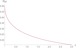
Figure 1: Numerical plot of the function $\bar{H}(p)$ for $\sigma=1$.

Example with a sextic potential.

As an illustration, let us investigate the case of a sextic potential (regarding the power of the variables $q_{i}$):

$$\mathcal{V}(x):=\frac{1}{3}h_{2}x^{3}+\frac{1}{2}h_{1}x^{2}+h_{0}x\,,$$ (33)

Furthermore, the equation for $\gamma$ is nothing but:

$$\ell(\gamma_{\pm})-2\sigma:=\frac{\partial\mathcal{V}}{\partial x}(\gamma_{\pm})\equiv 0\,,$$ (34)

and the two nonzero solutions are explicitly:

$$\gamma_{\pm}=-\frac{h_{1}}{2h_{2}}\pm\frac{\sqrt{h_{1}^{2}-4h_{2}h_{0}}}{2h_{2}}\,.$$ (35)

The coupling $h_{2}$ must be positive because of the stability requirement. Hence, if $h_{1}>0$, we have two configurations:

• For $h_{0}<0$, there is a single positive solution, $\gamma_{+}$.

• For $h_{0}>0$, the two solutions are negative or imaginary, and the low $T$ expansion does not exist.

For $h_{1}<0$ on the other hands,

• For $h_{0}>0$, as soon as $h_{1}^{2}>4h_{2}h_{0}$, there are two solutions for $\gamma_{\pm}$. There are no solutions for $h_{1}^{2}<4h_{2}h_{0}$.

• For $h_{0}<0$ finally, there are only one solution again, namely $\gamma_{+}$.

One can found on Figure 2 and illustration of this behavior for $h_{1}<0\,(=-3)$ and $h_{2}=1$, setting $\sigma=0.5$. For curves labeled from $(A)$ to $(D)$ , the value of the quadratic term $h_{0}$ decreases. Especially for the curve labeled by $(A)$, $h_{0}>0$ and the discriminant is negative, and as a result the solution set is empty ( the potential has a single minimum located for $x=0$). As $h_{0}$ decreases in $(B)$ to $(C)$, the discriminant becomes positive and two solutions appear. But as $h_{0}<0$, the first solution ultimately disappears leading us with a single solution, as the transition regime with phase coexistence is over.

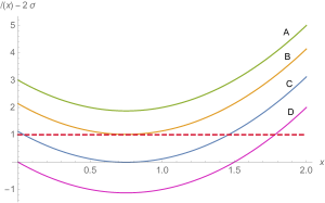
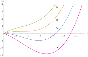
Figure 2: Solutions for $\gamma_{\pm}$ regarding the shape of the potential $\mathcal{V}(x)$ ($\sigma=1/2$).

III Convergence toward equilibrium points

In this section we investigate the validity of the previous assumptions, regarding especially the convergence toward equilibrium point for large $t$, that in particular will confirm the validity of the expected late time behavior for $G(t)$. Assuming the validity of the quenched limit, and because of the definition of $G(t)$, we have $\dot{G}(t)=2G(t)(\ell(t)-2\sigma)$, or explicitly:

$$\dot{G}(t)=2h_{K}G(t)\prod_{\mu=1}^{R}\left(\frac{H(t)+2TF(t)}{G(t)}-\gamma_{\mu}\right)^{r_{\mu}}\,,$$ (36)

where we set $h_{K}=1/2$ for simplicity, $R$ designates the number of zeros and $r_{\mu}$ their multiplicity. This is the equations that we will consider in this section.

Solution for quartic potential.

For a quartic potential, assuming $\gamma>0$ and setting $h_{1}=1/2$, the effective equation of motion for $G(t)$ reads:

$$\dot{G}(t)=-\gamma G(t)+H(t)+2TF(t)\,.$$ (37)

Once again, this equation can be solved using elementary Laplace transform techniques, and because of the initial condition $G(0)=1$, we get:

$$\bar{G}(p)=\frac{1+\bar{H}(p)}{p+\gamma-2T\bar{H}(p)}\,.$$ (38)

For small values of $p$, we find that the large-time dynamics is still dominated by the behavior of $\bar{H}(p)$, and the leading order contribution for $\bar{G}(p)$ is a slightly modified version of (29):

$$\bar{G}(p)=\frac{1/2}{T_{c}-T}\left[1+2\sigma-\frac{A(\sigma)T_{c}^{2}}{T_{c}-T}\left(1+\frac{2T}{\gamma}\right)\sqrt{p}\right]\,,$$ (39)

and again $G(t)\sim t^{-3/2}$ for late times (Theorem 1). Note that the critical temperature $T_{c}\equiv\gamma\sigma$ has the same value as in the static limit. The understanding of the global dynamics should require numerical methods. Focusing on the small temperature regime, one can make an expansion of the form:

$$G(t)=\sum_{n=0}^{\infty}\,(2T)^{n}G_{n}(t)\,,$$ (40)

and explicitly:

$$G_{0}(t)=e^{-\gamma t}+F_{0}(t)\,,$$ (41)

$$G_{1}(t)=\int_{0}^{t}G_{0}(t-t^{\prime})F_{0}(t^{\prime})\,,$$ (42)

with:

$$F_{0}(t):=\int_{0}^{t}H(t-t^{\prime})e^{-\gamma t^{\prime}}\,,$$ (43)

and for $n>0$ we have the general recursive relation:

$$G_{n}(t)=\int_{0}^{t}G_{n-1}(t-t^{\prime})F_{0}(t^{\prime})\,.$$ (44)

Figure 3 shows the behavior of $G_{0}(t)$ and $G_{1}(t)$ for $\sigma=\gamma=1$. Both have a maximum after which they decreases to $0$ as $t^{-3/2}$.

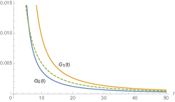
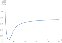
Figure 3: On the top: behavior of $G_{0}(t)$ and $G_{1}(t)$ for large time, the green dotted curve is $f(t):=0.16/t^{3/2}$. On the bottom: the behavior of $G_{0}(t)/G_{1}(t)$, that goes toward a constant for large time.

Higher potentials and degeneracy.

The case of a general potential having many minima could be difficult to investigate with elementary methods, excepts if we assume that the system is initially close to one the isolated minimums, say $\nu$,. In that case, one expect, because of the large depth of the well that the system remains close to this minimum during its dynamics. This can be achieved for instance by replacing our initial condition $q_{\lambda}(0)=1$ by $q_{\lambda}(0)=\sqrt{\Delta}$, such that $a(0)=\Delta$ and $|\Delta-\gamma_{\nu}|\ll 1$. Formally, assuming we remain close to the minimum $\gamma_{\nu}$ (that have to be checked to be self consistent) i.e. $|a(t)-\gamma_{\mu}|\equiv\epsilon(t)\ll 1$, and that spacing between minima is large enough, equation (36) rewrites as:

$$\frac{\dot{G}}{G}=2h_{K}R(\gamma_{\nu})r_{\nu}\left(\frac{\Delta H(t)+2TF(t)}{G(t)}-\gamma_{\nu}\right)+\mathcal{O}(\epsilon^{r_{\nu}+1})\,,$$ (45)

where $R(\gamma_{\nu})$ denotes the remaining of the euclidean division of $\ell(t)-2\sigma$ by $(a(t)-\gamma_{\nu})^{r_{\nu}}$, evaluated at the point $a(t)=\gamma_{\nu}$, and we can set $2h_{K}R(\gamma_{\nu})=1$ such that, close to the zero $\gamma_{\nu}$:

$$\dot{G}\approx G(t)\left(\frac{\Delta H(t)+2TF(t)}{G(t)}-\gamma_{\mu}\right)^{r_{\nu}}\,.$$ (46)

For $r_{\nu}=1$, excepts for the $\Delta$ in front of $H(t)$, we recover exactly what we obtained for the quartic case, and we investigate the case $r_{\nu}>1$ in the rest of this paragraph.

The behavior of the system will be different for odd or even values of $r_{\mu}$. Let us consider the case of an even value, and especially the case $r_{\mu}=2$:

$$\dot{G}=G(t)(a(t)-\gamma)^{2}\,.$$ (47)

In that case, because $G(t)$ is a positive function, $\dot{G}>0$ and the function $G(t)$ increases for all times. For $T=0$, it is easy to check that $G(t)=e^{\alpha t}$ is an asymptotic solution for the dynamics provided that $\alpha=\gamma^{2}$. This can be checked numerically, and the late time behavior of the system is pictured on Figure 4 ($G_{\text{num}}(t)$ denoting the numerical solution of the equation). If we assume the system converge to some finite value $a_{\infty}$, we must have: $(a_{\infty}-\gamma)^{2}=\gamma^{2}$. The condition $a_{\infty}=0$ that solve this equation means the system goes toward the zero ”vacuum” because of the disorder.

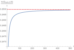
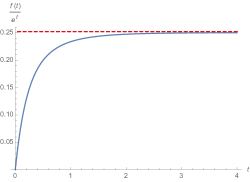
Figure 4: On the top: numerical behavior of $G(t)$ at $T=0$ for large $t$ with $\sigma=1$ and $\gamma=0.5$. On the bottom, behavior of $f(t)e^{-t}$ for $\sigma=1$ and $a^{2}=1$.

For small $T$, one expect that the exponential behavior holds, and indeed:

$$f(t):=\int_{0}^{t}H(t-t^{\prime})e^{a^{2}t^{\prime}}\sim Q(a^{2},\sigma)e^{a^{2}t}\,,$$ (48)

where explicitly:

$$Q(a^{2},\sigma):=\frac{-a\sqrt{a^{2}+8\sigma}+a^{2}+4\sigma}{8\sigma^{2}}\,.$$ (49)

Hence, asymptotially, the equilibrium value for $a^{2}$ is given by the solutions of the equation :

$$a^{2}=(2TQ(a^{2},\sigma)-\gamma)^{2}=:Y(a,\sigma,\gamma,T)\,,$$ (50)

and the dependency on $T$ of the solution is illustrated on Figure 5. The existence of a transition temperature that signal the end of the exponential regime can be proved by the following argument. Let $G(t)=\mathcal{A}(t)e^{a^{2}_{*}t}$ such that $\mathcal{A}(0)=1$ and $a^{2}_{*}$ a solution of equation $a^{2}=Y(a,\sigma,\gamma,T)$. Assuming $a(t)\ll 1$ accordingly with our zero temperature analysis, we have:

$$\dot{\mathcal{A}}\simeq-2\gamma\mathcal{A}(t)a(t)+\mathcal{A}(t)\delta\gamma^{2}\,,$$ (51)

where $\delta\gamma^{2}:=\gamma^{2}-a^{2}_{*}$. Introducing $\mathcal{B}(t):=\mathcal{A}(t)e^{-\delta\gamma^{2}t}$, the effective equation for $\mathcal{B}(t)$ can be still solved by Laplace transform; and we get:

$$\bar{\mathcal{B}}(p)\simeq\frac{1-2\gamma\Delta\bar{H}(p+\gamma^{2})}{p+4\gamma T\bar{H}(p+\gamma^{2})}\,.$$ (52)

Hence, for large $t$, one expect the following behavior:

$$\mathcal{B}(t)\sim e^{-4\gamma T\bar{H}(\gamma^{2})t}\,,$$ (53)

and $G(t)$ increases exponentially provided that:

$$T<T_{c}\simeq\frac{\gamma}{4\bar{H}(\gamma^{2})}\,.$$ (54)

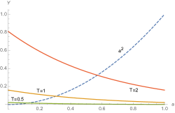
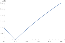
Figure 5: On the top: Graphical solution of the equation for $\sigma=1$ and $\gamma=0.1$. On the bottom: explicit dependency of $a(T)$ on the temperature for $\gamma=0.1$.

To conclude, let us investigate the case of an odd value for $r_{\mu}$, focusing on $r_{\mu}=3$ for numerical study. The typical behavior of $G_{\text{num}}(t)$ for $T=0$ is showed on Figure 6, assuming $\Delta$ such that initial condition is close enough to the degenerate vacuum. Numerically one find that the system behaves as $G_{\text{num}}(t)\sim e^{-\gamma^{3}t}$ for late time. Once again, a transition temperature can be estimated by the following argument. The equilibrium equation $(a(t)-\gamma)^{3}=-\gamma^{3}$ admits in particular the unstable zero $a=0$. Hence, assuming $a(t)\sim 0$, the equation can be linearized, and one find that the system goes toward the non zero vacuum $a=\gamma$ as $1/t$, provided that $T<T_{c}=\gamma^{3}/2\bar{H}(0)$.

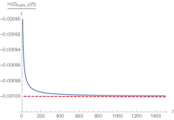
Figure 6: Behavior of $G_{\text{num}}(t)$ for late time, with $\sigma=1$ and $\Delta=\gamma=0.1$

IV Summary and outlooks

In this paper we investigated the low temperature behavior of the asymptotic quenched dynamics for a $p=2$ soft spin model with polynomial confining potential. We showed that a closed equation for $a(t)$ arises in the quenched limit, which is difficult to solve, and a first part of our analysis was devoted to a systematic analysis of the asymptotic closed equation for $G(t)$ arising from the assumption that the system relaxes toward one of the equilibrium points of the potential. The assumption that the solution of this equation provides the true asymptotic behavior for the function $G(t)$ is consistent only below a critical value $T<T_{c}$ for the temperature, and in this regime the closed equation can be solved using Laplace transform methods. This leads to a power law $G(t)\sim t^{-3/2}$, and $\ell(t)\sim 2\sigma+\mathcal{O}(t^{-1})$. Besides the assumption that the system has small fluctuations around some zero of the function $\ell(t)-2\sigma$ and that $H(t-t^{\prime})$ suppress small times contributions for $G(t^{\prime})$ on the left hand side of the closed equation, the method assumes the existence of the Laplace transform of the function $G(t)$. Hence, the failure of the method above the critical temperature ($T>T_{c}$) is interpreted as the failure of the assumption about the existence of the Laplace transform, and $G(t)$ is assumed to increases exponentially at this point, corresponding to an exponential relaxation toward equilibrium. These results accompany those of the reference Vincent , which aims to construct a reliable renormalization group for this model.

In the second part of this paper, we investigated the validity of our assumptions for the closed equations for $G(t)$, and we study the way the system converges toward equilibrium points using effective dynamics for the quenched variable $a(t)$. We thus elucidate the behavior of $\dot{G}(t)$, and especially the dependency of the previous assumption regarding the order of the zeros of the potential. In this way, we show that for zeros with multiplicity one, the conclusions of the previous section holds, and the system below the critical temperature reaches equilibrium with rate $t^{-1}$, and has power law late time correlations. In the general case however, the late time behavior is not the same for odd and even multiplicity. For odd multiplicities, the behavior is essentially the same as for multiplicity one, and after an exponential phase, $G(t)$ behaves as $t^{-3/2}$ for large times. When multiplicity is even in contrast, $G(t)$ diverges exponentially also for zero temperature, and the previous assumption regarding the role of thermal fluctuation is wrong: The system fails to have a power law decays at $T=0$, and due to elementary properties of convolutions, this holds for temperature small enough. One can furthermore provides an estimate of the temperature where the system fails to reach the effective equilibrium point $a(t)=0$.

Many of the conclusions of this paper strongly depend on the crude large $N$ limit, and it should be interesting to evaluate finite $N$ effects, regarding for instance the activation of metastable states due to thermal fluctuations (the famous Kramer’s problem, see for instance Chupeau ; Burada ; Visscher ; Berera ; Melnikov ; Kamenev . Furthermore, some approximations used in his paper allow only to provide an estimate of transitions temperature, and should be improved.

References

- (1) I. G. Cirano De Dominicis. Random Fields and Spin Glasses: A Field Theory Approach. Cambridge University Press, 2009.
- (2) L. F. Cugliandolo, David S. Dean, Full dynamical solution for a spherical spin-glass model, J. Phys. A 28 4213 (1995).
- (3) K. van Duijvendijk, R. L. Jack, and F. van Wijland, Second-order dynamic transition in a p=2 spin-glass model, Phys. Rev. E 81, 011110 – Published 8 January 2010.
- (4) K. van Duijvendijk, Robert L. Jack, and Frédéric van Wijland, Second-order dynamic transition in a p=2 spin-glass model, Phys. Rev. E 81, 011110 – Published 8 January 2010.
- (5) H. Nishimori. Statistical Physics of Spin Glasses and Information Processing: An Introduction. Oxford Scholarship Online, 2010.
- (6) L. F. Cugliandolo. Dynamics of glassy systems. In: Lecture notes, Les Houches (2002).
- (7) J. Kurchan, L. F. Cugliandolo. Analytical Solution of the Off-Equilibrium Dynamics of a Long Range Spin-Glass Model. In: Phys. Rev. Lett. (1993).
- (8) J. K. M. M. Jean Philippe Bouchaud Leticia F Cugliandolo. “Out of equilibrium dynamics in spin-glasses and other glassy systems.” In: Spin-glasses and random fields, A. P. Young Ed. (World Scientific) (1997).
- (9) C. Aron, G. Biroli, and L. F. Cugliandolo. “Symmetries of generating functionals of Langevin processes with colored multiplicative noise.” In: Journal of Statistical Mechanics: Theory and Experiment 2010.11 (2010), P11018. issn: 1742-5468.
- (10) Y. V. Fyodorov, A. Perret, and G. Schehr. Large time zero temperature dynamics of the spherical p= 2-spin glass model of finite size. In: Journal of Statistical Mechanics: Theory and Experiment 2015.11 (2015), P11017.
- (11) M. Rokni and P. Chandra. “Dynamical study of the disordered quantum p= 2 spherical model.” In: Physical Review B 69.9 (2004), p. 094403.
- (12) A.J. Bray, Theory of phase-ordering kinetics, Advances in Physics Volume 43, 1994 - Issue 3.
- (13) C. L. Emmott and A. J. Bray, Phase-ordering dynamics with an order-parameter-dependent mobility: The large-n limit, Phys. Rev. E 59, 213 – Published 1 January 1999.
- (14) M. Potters, J-P. Bouchaud, A First Course in Random Matrix Theory for Physicists, Enginneers and Data Scientifics, Cambridge University Press, 2021.
- (15) M. Mézard, G. Parisi, N. Sourlas, G Toulouse, and M. Virasoro. Nature of the spin-glass phase. Physical review letters 52.13 (1984), p. 1156.
- (16) A. Caiazzo, A. Coniglio, and M. Nicodemi. “Glass glass transition and new dynamical singularity points in an analytically solvable p-spin glass like model.” In: Phys. Rev. Lett (2004).
- (17) R. A. Handelsman, J. S. Lew, Asymptotic expansion of Laplace transforms near the origin, Siam J. Math. Anal, Vol. 1 1, 1970.
- (18) V. Lahoche, D. Ousmane Samary, M. Tamaazousti, Functional renormalization group for multilinear disordered Langevin dynamics II: Revisiting the spin dynamics for Wigner and Wishart ensembles, arXiv:2212.05649 [hep-th].
- (19) A. Altieri,G. Biroli and C. Cammarota, Dynamical mean-field theory and aging dynamics. Journal of Physics A: Mathematical and Theoretical, 53(37), 375006, (2020).
- (20) V. Lahoche, D. Ousmane Samary and M. Ouerfelli, Functional renormalization group for multilinear disordered Langevin dynamics I Formalism and first numerical investigations at equilibrium. Journal of Physics Communications, 6(5), 055002, (2022).
- (21) V. Lahoche, D. Ousmane Samary and M. Ouerfelli and M. Tamaazousti, Field theoretical approach for signal detection in nearly continuous positive spectra II: Tensorial data. Entropy, 23(7), 795, (2021).
- (22) V. Lahoche, D. Ousmane Samary, M. Tamaazousti, Signal Detection in Nearly Continuous Spectra and -Symmetry Breaking. Symmetry, 14(3), 486, (2022).
- (23) V. Lahoche, D. Ousmane Samary, M. Tamaazousti, Field theoretical approach for signal detection in nearly continuous positive spectra I: matricial data. Entropy, 23(9), 1132, (2021).
- (24) V. Lahoche, D. Ousmane Samary, M. Tamaazousti, Generalized scale behavior and renormalization group for data analysis. Journal of Statistical Mechanics: Theory and Experiment, 2022(3), 033101, (2022).
- (25) M. Chupeau, J. Gladrow, A. Chepelianskii, U.F. Keyser and E. Trizac, Optimizing Brownian escape rates by potential shaping. Proceedings of the National Academy of Sciences, 117(3), 1383-1388, (2020).
- (26) P. B .Burada and B. Lindner, Escape rate of an active Brownian particle over a potential barrier. Physical Review E, 85(3), 032102, (2012).
- (27) P. B. Visscher, Escape rate for a Brownian particle in a potential well. Physical Review B, 13(8), 3272, (1976).
- (28) A. Berera, J. Mabillard, B.W. Mintz, and R.O. Ramos, Formulating the Kramers problem in field theory. Physical Review D, 100(7), 076005, (2019).
- (29) V. I. Melnikov, The Kramers problem: Fifty years of development. Physics Reports, 209(1-2), 1-71, (1991).
- (30) A. Kamenev, Field theory of non-equilibrium systems. Cambridge University Press, (2023).