Optimal spectral lines for measuring chromospheric magnetic fields

Abstract

This paper identifies spectral lines from X-ray to infrared wavelengths which are optimally suited to measuring vector magnetic fields as high as possible in the solar atmosphere. Instrumental and Earth’s atmospheric properties, as well as solar abundances, atmospheric properties and elementary atomic physics are considered without bias towards particular wavelengths or diagnostic techniques. While narrowly-focused investigations of individual lines have been reported in detail, no assessment of the comparative merits of all lines has ever been published. Although in the UV, on balance the Mg⁺ $h$ and $k$ lines near 2800 Å are optimally suited to polarimetry of plasma near the base of the solar corona. This result was unanticipated, given that longer-wavelength lines offer greater sensitivity to the Zeeman effect. While these lines sample optical depths photosphere to the coronal base, we argue that cores of multiple spectral lines provide a far more discriminating probe of magnetic structure as a function of optical depth than the core and inner wings of a strong line. Thus, together with many chromospheric lines of Fe⁺ between 2585 and the $h$ line at 2803 Å, this UV region promises new discoveries concerning how the magnetic fields emerge, heat, and accelerate plasma as they battle to dominate the force and energy balance within the poorly-understood chromosphere.

1 Introduction

The solar atmosphere, comprising those outermost regions from which radiation freely escapes into space, exhibits many phenomena related to the emergence of magnetic fields generated in the interior. While less than 1 part in 1000 of the solar luminosity is associated with these magnetic fields, their effects can be dramatic, being dynamically dominant in the tenuous chromospheric and coronal plasmas (reviewed, for example, by Eddy, 2009). To understand mechanisms behind these phenomena, we must measure magnetic fields above the visible surface, the “photosphere”. We are obliged to measure the magnetic field vector, not merely components such as the vector projected on to the line-of-sight (LOS), because the free magnetic energy driving flares and coronal mass ejections (CMEs) depends on the electric currents $\mathbf{j}=\nabla\times\mathbf{B}$ threading the plasmas.

To determine $\mathbf{j}$ using spectral lines requires measurements of linearly and circularly polarized line profiles, as well as unpolarized intensity (Landi degl’Innocenti & Landolfi, 2004). While the line-of-sight component of j can be fixed from measurements of B in a plane perpendicular to the line-of-sight (LOS) (e.g. Pevtsov & Peregud, 1990; Metcalf et al., 1994), the perpendicular components require measuring features formed elsewhere along each LOS, preferably in a second spectral line. Different strategies can be used to map measured polarization states to magnetic field vectors. All require various assumptions and approximations. One strategy is to perform “inversions”, which iteratively modify a model magnetized atmosphere until a match to observations is found. In this way Socas-Navarro (2005a, b) inverted Zeeman-induced polarization observed in photospheric Fe and chromospheric Ca⁺ 8542.1 Å lines. With his instrumentation and choice of spectral lines, he could derive $\mathbf{j}$ only on scales $\geq$ 1Mm. The measurement is crude because the entire stratified chromosphere spans only 1.5 Mm (Vernazza et al., 1981). Examples of more recent measurements of j are photospheric work by Pastor Yabar et al. (2021) and chromospheric work by Anan et al. (2021).

Common to all such studies, the measurements must be augmented with a variety of more-or-less credible assumptions and even ad-hoc procedures to “fill in” information missing from the data themselves. “Regularization” is a well-known but subjective example employed in the inverse strategy (e.g. Craig & Brown, 1976). Pure data therefore become laden with impurities, assumptions, some explicit (e.g., in the work of Socas-Navarro, the atmosphere is in hydrostatic equilibrium), others implicit (e.g., use of a small number of “nodes” at which numerical solutions for physical quantities are sought). However, the chromosphere is incompatible with many simplifying assumptions commonly applied to the photosphere (LTE, Milne-Eddington solutions, statistical equilibrium) or the corona (optically thin). Our understanding of chromospheric magnetic fields and their interaction with plasma is accordingly rudimentary. We do not yet know how the chromosphere modulates magnetic energy emerging through the photosphere before reaching the corona.

Given these challenges, we undertook a search for information-rich lines in the solar spectrum, in the hope of maximizing the magnetic information content of remotely sensed magnetic fields. Our search is conducted without bias towards specific wavelengths or observing platforms, for the first time.

2 Requirements

We seek spectral lines only of atoms and atomic ions. Molecules, useful in the deep photosphere, will be ignored because their population densities drop to negligible values, exponentially with half of the pressure scale height of the plasma (itself just $\approx 150$ km). Photospheric magnetic fields vary from a few G, to as much as several thousand G in the cores of sunspots. Being farther from sub-photospheric sources of electric currents, chromospheric magnetic fields generally are weaker.

The lines of most interest must:

• be able to reveal signatures of solar magnetic fields down to 1G, without specialization to a specific physical origin,

• be able to constrain the vector field B, not just a component of it,

• be sufficiently opaque to form within the higher, more tenuous plasma in and above the solar chromosphere,

• have opacities simply related to atmospheric pressures and temperatures, to fix relative heights of formation,

• be readily observable with current instruments,

• be bright enough to achieve signal-to-noise ratios sufficient to interpret the magnetic signatures.

The final criterion is of first importance, because spectropolarimetry is photon-starved, even on the Sun’s bright disk (Landi Degl’Innocenti, 2013). The third criterion demands the use of very strong (i.e. opaque) lines, which traditionally have been poorly understood. However, recent work has shed light on the formation of both intensity (Judge et al., 2020) and polarization (Manso Sainz et al., 2019) of such lines. The fourth criterion is not satisfied for lines of H and He between any excited levels (e.g. H Balmer $\alpha$ and He 10830 Å).

Generally, any measured signals should also be stable against instrumental fluctuations and degradation, and the negative effects of a variable terrestrial atmosphere (extinction, scattering, seeing). Polarimetry requires multiplexed simultaneous measurements to avoid spurious noise and cross-talk, setting requirements on integration times for modulation and demodulation, which can conflict with rapid evolution of the solar plasmas and SNR requirements (Lites, 1987; Judge et al., 2004; Casini et al., 2012). Continuity and regular repeatability of observations over periods up to months is highly desirable, to follow evolution of emerging fields, wave motions, and the explosive release of magnetic free energy stored within the atmosphere over extended periods. The evolution of magnetism in active regions and coronal holes, for example, demands extended observations over hours to months. The day/night and seeing cycles, as well as weather events, present challenges at most ground-based observatories. Thus operations in space, necessary for UV and some infrared observations, should perhaps be favored.

These considerations point to the primary requirement for this study: the spectral lines must be as bright as possible.

3 Solar and atomic properties

3.1 Elemental abundances

The need for strong, opaque spectral lines limits the selection to a subset of roughly 10-15 elements. Those with abundances above $10^{\mathrm{-5}}$ of hydrogen are (Allen, 1973):

H, He,
C, N, O, Ne,
Mg, Si, S, Ar,
Ca, Fe,

where the elements are grouped according to the row that they occupy in the periodic table. Of these, all elements have stable dominant isotopes with even numbers of nucleons except for H and N. Consequently, both H and N have nuclear-spin-induced hyperfine structure, introducing higher levels of complexity into current models, which have yet to be generally implemented (Alsina Ballester et al., 2016).

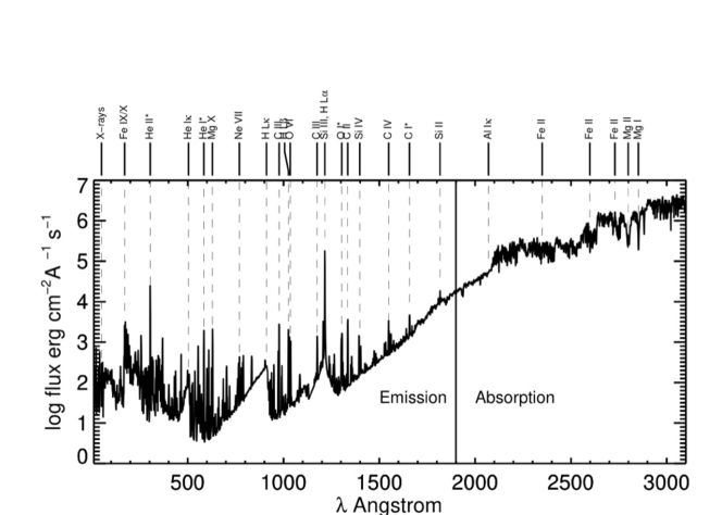
Figure 1: The solar flux spectrum as measured on Mar 25-29 2008 with various instruments, compiled by staff at LASP as part of the Whole Heliospheric Interval Campaign, from http://lasp.colorado.edu/lisird/. The spectrum is from soft X-rays to near the atmospheric cut-off, highlighting emission and absorption features. The region has a number of deep absorption lines with emission in their core. Mg II is such an example, although the emission is not observable due to the modest spectral resolution. The transitions of H, He I and He II, with $\Delta n=1$ and are labeled with asterisks are compared with $\Delta n=0$ transitions of much more highly ionized species at similar wavelengths.

3.2 Atmosphere

The Sun’s atmosphere is a continuously evolving, partially or fully ionized plasma threaded by magnetic fields. The pressure in the line-forming region of the photosphere happens to be about $10^{\mathrm{4}}$ dyne cm^-2, in the corona it varies from about $0.2$ to 10 dyne cm^-2 under conditions of extreme heating in active regions. Temperatures in these regions are $\approx$5000 K (upper photosphere), and from $10^{\mathrm{6}}$ to say $3\times 10^{\mathrm{6}}$ K (corona), outside of flares.

The intervening chromosphere, spanning about 9 pressure scale heights, is stable to temperature fluctuations driven by over- heating, most excess energy going to latent heat of ionization, powerful radiation losses and some into plasma motions. Standard models (e.g. Vernazza et al., 1981) place its temperature near 6000-8000 K ($\equiv 0.5$ eV) across these changes in pressure, with an almost constant electron pressure of $0.1$ dyne cm^-2 but with partial pressures of neutral hydrogen varying from $1000$ to $0.1$ dyne cm^-3.

The average pressure drop with height has a direct impact on our selection of spectral lines. The vast bulk of the chromosphere must be close to hydrostatically stratified given the observed sub-sonic motions (outside of a tiny fraction of area from which spicules emerge, Judge, 2010). Thus, on average, pressure supports the weight of material above it:

$$p=mg$$ (1)

where $m=\int\rho dz$ (g cm^-2) is the column mass, and $g$ the solar acceleration due to gravity. The line center optical depths $\tau_{\mathrm{0}}$ of many spectral lines are indeed simply related to the column mass $m$ (fourth requirement listed in section 2). For a given internal state of excitation of the radiating or absorbing ion (Mihalas, 1978, ignoring stimulated emission, and using standard notation):

$$\tau_{\mathrm{0}} = \frac{\pi e^{\mathrm{2}}}{m_{\mathrm{e}}c}f_{\mathrm{ij}}\ \int n_{\mathrm{i}}\phi(\nu_{\mathrm{0}})dz,\ \mathrm{where}$$ (2)

$$\int n_{\mathrm{i}}dz = \int\left\{\frac{n_{\mathrm{i}}}{n_{\mathrm{ion}}}\frac{n_{\mathrm{ion}}}{n_{\mathrm{el}}}\frac{n_{\mathrm{el}}}{n_{\mathrm{H}}}\frac{n_{\mathrm{H}}}{\rho}\right\}\ \rho dz,$$ (3)

where $\phi(\nu_{\mathrm{0}})$ is the line profile function at line center frequency $\nu_{\mathrm{0}}$, and the term in braces simply expresses the number density in the lower level as a fraction of the total plasma density. If both quantities are roughly constant along the line of sight $z$, then $\tau_{\mathrm{0}}\propto m$, thereby satisfying requirement 4 of section 2. Not all lines in the solar spectrum satisfy this criterion.

Between chromospheric and coronal plasma is the intermediate temperature “transition region” with very little plasma owing to the large average temperature gradient there. The majority of “transition region” lines are optically thin, with the exceptions of resonance transitions of H and He.

3.3 Spectrum

Most spectral lines observed from visible to infrared wavelengths (henceforth “vis-IR”) form as narrow absorption features in the photosphere. Near-LTE conditions characteristic of high pressure plasma ensure that the dominant ionization stages are neutrals (H, He, O, Ne) or, for elements with lower ionization potentials, singly ionized (e.g., Mg⁺, Ca⁺, Fe⁺). Between the lines is the near-black-body continuum, formed as the H^- ion becomes optically thin at plasma pressures near 10⁵ dyne cm^-2, with a characteristic radiation temperature near 5770 K.

Vis-IR lines are generally weak, because they mostly originate from between excited atomic levels, with small populations and little opacity. The line spectrum of neutral iron dominates by number the visual solar spectrum, yet even the resonance lines ($4s-4p$ transition array) near 3720 Å, are a factor of 500 less opaque than the $4s-4p$ transitions in Fe⁺ near 2600 Å, because of smaller oscillator strengths (see below) and different chromospheric ion populations $n_{\mathrm{ion}}/n_{\mathrm{Fe}}$.

One exception is hydrogen, which is abundant enough to generate significant photospheric opacity in transitions between excited levels (with principal quantum number $n\geq 2$) to generate deep absorption lines. Resonance lines lie at UV and vacuum UV wavelengths, except in lithium, sodium and potassium-like ions. Their $ns-np$ transitions (note the same value of $n$) are strong electric dipole (E1) transitions between levels separated only by the residual electrostatic interaction, and not the central Coulomb field. The resonance lines of Li-like sequence of ions are clearly identified as C IV, N V, O VI, Ne VIII and Mg X in Figure 1. The $3s-3p$ sodium D lines lie at 5800 Å, and the Na-like Ca⁺ $H$ and $K$ lines, the two strongest lines in the vis-UV spectrum, lie at 3969 and 3934 Å. (Throughout we use air wavelengths above 2000 Å, vacuum below). Ca⁺ also has a trio of less opaque lines near 8542 Å, sharing a common upper level with $H$ and $K$, decaying to a metastable level 1.7eV above the ground levels. These lines have cores forming in the mid chromosphere ($p\approx$ 1 dyne cm^-2).

At wavelengths below the Balmer continuum (3650 Å), absorption lines of complex ions of the iron group dominate in number, and they generally have higher opacities than vis-IR transitions. The unfilled $3d$ shell has many meta-stable levels as the equivalent hydrogen’s “ground level” is split into multiple levels with the same parity. These levels are highly populated, with modest energies $\approx 1-2$ eV above the lowest level.

Below about 2000 Å, the spectrum changes character as line opacities become mixed with photoionization continuum opacities of abundant elements, formed well above the photosphere near $p\approx 10^{\mathrm{3}}$ dyne cm^-2 (Vernazza et al., 1981). The spectrum is superposed with the well-known emission lines originating from heated and warmer plasma lying above the continuum formation regions, and at yet lower pressures.

Table LABEL:tab:calcs lists only the brightest lines in the solar spectrum which are formed well above the photosphere, for further scrutiny below. Absent are well-known weaker magnetically-sensitive lines of abundant neutrals of the iron group, and also even “chromospheric” resonance lines of neutrals, such as Ca 4227 Å. Owing largely to ionization balance (see below), the latter is formed in dense, high pressure plasma ($p_{\mathrm{plasma}}\approx 20$ dyne cm^-2), typically 1000 km beneath the corona (Bianda et al., 2011).

3.4 States of ionization

The requirement to use the strongest lines has consequences dictated by the solar plasma temperatures, and densities, which primarily determine the dominant stages of ionization in the atmosphere (factor $n_{\mathrm{ion}}/n_{\mathrm{el}}$ in equation 3). In the deepest, highest pressure chromospheric layers, ionization equilibrium is almost controlled through the principle of micro-reversibility leading to LTE. The ionization occurs via impact of ambient plasma electrons on atomic ions (one electron before, two after the collision), balanced by the reverse thermodynamic process of 3-body recombination (two electrons impacting the ion, one free electron after the collision). The ionization follows Saha’s formula, and consequently neutral atoms with ionization potentials less than about 8eV tend to be fully ionized. For other abundant elements, neutral species are also ionized by solar radiation at UV and EUV wavelengths. Except for H, He and some noble gases with high ionization potentials, the dominant stage of ionization across the chromosphere is X⁺ for most elements X.

The spectral lines of interest form in higher, much less dense plasmas where LTE does not apply. Only 2-body collisions are then important, so that ionization by electron impact is balanced by radiative plus dielectronic recombination. In this “coronal” regime, ionization fractions are essentially simple functions of electron temperature (Woolley & Allen, 1948)). The LTE and coronal ionization regimes are clearly illustrated in an early review by Cooper (1966). As a rule of thumb, atomic ions with net charge $z$ have a maximum abundance near electron temperatures

$$T_{\mathrm{e}}\approx 10^{\mathrm{4}}z^{\mathrm{2}},$$ (4)

a rough approximation when $T_{\mathrm{e}}>10^{\mathrm{4}}$ K, based upon general formulae balancing electron impact ionization and radiative recombination. Thus, 3$\times$ ionized ions would form near $10^{\mathrm{5}}$K, those $10\times$ ionized near $10^{\mathrm{6}}$K, temperatures of the mid transition region and quiet corona respectively.

3.5 Atomic physics

For solar applications we seek radiative signatures from fields as weak as $1$ G, and as strong as a few kG, within the chromosphere and corona. A field of magnitude $B=|\mathbf{B}|$ acting on a (non-degenerate) level produces an energy splitting of order $\mu_{\mathrm{B}}B$ (Zeeman splitting) where $\mu_{\mathrm{B}}$ is the Bohr magneton, and an alignment of the gyrating atom along $\mathbf{B}$. In the absence of spin-induced hyperfine structure (elements H, N) or anomalously close levels, the fine-structure splitting greatly exceeds the Zeeman splitting for most solar magnetic fields. In such cases, one can exploit the familiar perturbation formulation of the Zeeman effect. Cowan (1981) lists dependencies of fine-structure splittings under various scenarios, also as a function of net charge $z$, varying as $(z+1)^{\mathrm{\alpha}}$ with various values of $\alpha>2$.

The magnetic splitting and associated alignment (breaking of symmetry) leads to polarized spectral lines even if the lines are far narrower than the thermal line width. Then, the magnitude of the Zeeman-induced polarization depends on the quantity $\varepsilon\approx\mu_{\mathrm{B}}B/\Delta E$, where $\Delta E$ is the width of the spectral line in energy units. For a plasma temperature of $T$ K and an ion of mass $m$, we have for a Doppler dominated line

$$\varepsilon\approx\frac{\mu_{\mathrm{B}}B}{\Delta E}=\frac{\mu_{\mathrm{B}}B}{\sqrt{kT/m}}\frac{\lambda}{h}\ll 1.$$ (5)

For energy splittings small compared with fine structure and line widths, Zeeman-induced circularly polarized light varies as $\varepsilon^{\mathrm{1}}$, linear polarization varies as $\varepsilon^{\mathrm{2}}$ (Landi degl’Innocenti & Landolfi, 2004). This familiar result favors longer-wavelength lines of heavier ions formed in lower temperature plasmas. All three factors lead to a higher sensitivity to the Zeeman effect.

Sometimes $\mu_{\mathrm{B}}B$ is comparable to fine structure energies when accidental atomic level crossings are present, as occurs in some complex ions. In this case, the mixing of two otherwise “pure” atomic states by even a modest magnetic field can give rise to an otherwise completely absent spectral line (magnetically induced transition, or MIT). The new line’s intensity varies as $B^{\mathrm{2}}$. Such a mixing has led to a proposal (Grumer et al., 2014; Li et al., 2016; Si et al., 2020a) to examine the EUV spectrum of chlorine-like ion Fe X, and Si et al. (2020b); Landi et al. (2020) have recently used this method to estimate magnetic field strengths in coronal plasmas. This method has several practical challenges such as line blending in the EUV, sensitivity to $B=|{\mathbf{B}}|$ and using lines which are optically thin so that information along the LOS is almost absent. Thus we seek other diagnostic techniques.

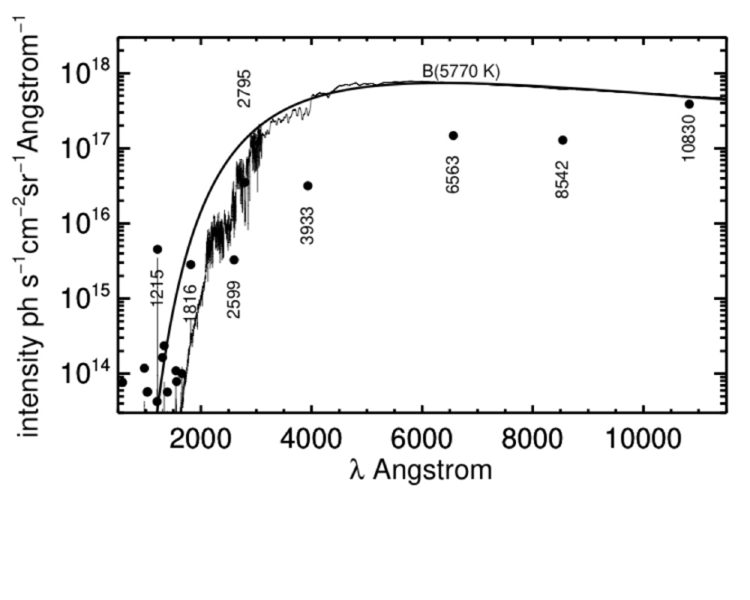
Figure 2: Intensities in the cores of the strongest lines are plotted, together with a black body spectrum at the solar effective temperature for reference. Also shown is a modest (typically 2Å) resolution intensity spectrum from the Whole Heliosphere Interval campaign (https://lasp.colorado.edu/lisird/data/whi$_{–r}}$ef$_{–s}}$pectra), derived as $1/\pi$ of the irradiance spectrum scaled to the solar surface. Line core intensities (filled circles) used here and their sources are listed in Table LABEL:tab:calcs.

The less familiar Hanle effect exploits the modification by magnetic fields of pre-existing spectral-line polarization produced by resonance scattering. Scattering polarization originates even in the absence of external fields, through excitation processes that are anisotropic, such as irradiation of atoms by light coming from a preferred direction, or by non-isotropic collisions. Further, the associated atomic sub-levels evolve coherently as their wavefunctions are mixed (entangled), their levels being degenerate in the absence of external fields.

While a rigorous treatment of the Hanle effect requires quantum electrodynamics (Landi degl’Innocenti & Landolfi, 2004), a classical picture illustrates the energy regime in which magnetic fields influence the polarization of the scattered radiation. During a time of order $A^{\mathrm{-1}}$ necessary for an excited level to decay radiatively (where $A$ is the Einstein coefficient for spontaneous emission), the classical damped electron oscillator precesses around the magnetic field with the Larmor frequency

$$\omega_{\mathrm{B}}=\frac{\mu_{\mathrm{B}}}{\hbar}B,$$ (6)

where $\mu_{\mathrm{B}}$ is Bohr’s magneton, Then the mean linear polarization of the radiation emitted by the damped oscillator will generally be rotated and reduced in amplitude with respect to the field-free case. The Hanle effect is thus sensitive to magnetic field strengths $B$ of order

$$B_{\mathrm{H}}\sim\frac{\hbar A}{\mu_{\mathrm{B}}}$$ (7)

With $A\sim 10^{\mathrm{8}}$ s^-1 for a typical E1 transition, $\mu_{\mathrm{B}}\approx 10^{\mathrm{-20}}$ erg G^-1, then

$$B_{\mathrm{H}}\sim 10^{\mathrm{-7}}A\,\ \ \ \mathrm{Gauss}.$$ (8)

For lines of ions in an isoelectronic sequence, $B_{\mathrm{H}}$ values can be estimated in plasmas at temperatures given by eq. (4) from

$$A(z)\approx A(z=0)z^{\mathrm{\alpha}},$$ (9)

with $\alpha=4$ or 2 for E1 transitions with (a or no) change in principal quantum number respectively. In the L_α line of He⁺, formed near 10⁵ K for example, the critical fields are larger than for H L_α by a factor of 16 (see Table LABEL:tab:calcs, which also contains $\overline{G}$, the Zeeman factor for linear polarization of Landi degl’Innocenti & Landolfi, 2004).

4 Analysis

In bringing together the previous sections we can identify the most promising spectral lines for measuring those magnetic configurations well above the photosphere, which cause flares, heating, and plasma eruptions.

4.1 A first cut

Figure 2 shows estimates of the line core intensities, in photon units, compiled in Table LABEL:tab:calcs. The cores are our focus for two reasons: they form highest, and the Hanle effect operates in the Doppler cores. By far the lines with highest photon fluxes are, in order, He 10830, Mg⁺ 2795 and 2803, H B$\alpha$ 6563, Ca⁺ 3933 and 8542, H L$\alpha$ 1216, a multiplet of Si$+$ whose strongest line is at 1817 Å, and resonance lines of Fe⁺ between 2585 and 2632 Å. These are all chromospheric lines, not surprising because the chromosphere radiates far more energy than the transition region and corona (Withbroe & Noyes, 1977). Our first cut therefore includes only these lines, all of which, when observed against the solar disk, are optically thick in the chromosphere. The exception is He 10830, a weak absorption line, barely visible outside of active regions, whose origin is still a subject for debate (compare abstracts of papers by Judge & Pietarila, 2004 “the spatio-temporal properties of the He I 584 Å… are qualitatively unlike other chromospheric and transition region lines”, and that of Leenaarts et al., 2016), “the basic formation of the line in one-dimensional models is well understood”. Although the first paper focuses on resonance lines and the latter on 10830, both EUV and IR lines of helium require excitation to levels inaccessible to electrons at local thermal energies. Further, Leenaarts et al. (2016) did not recognize the failure of one-dimensional models to explain anomalous Doppler shifts of the 10830 Å line (Fleck et al., 1994) which are in phase with the well understood Ca II $K$ line. The optical depths listed in Table LABEL:tab:calcs can be scaled to solar values, they are all relative to H L$\alpha$, computed from identical geometrical depth of 100 km and electron and hydrogen densities of 10¹¹ particles cm^-3 with the additional assumption that each ion listed has $n_{\mathrm{ion}}/n_{\mathrm{el}}=1$ (equation 3). No microturbulence was included in the line profiles. In the Sun the plasma path lengths vary from Mm in the chromosphere, which also has higher neutral densities, to below 100 km in the steepest part of the transition region, with at least 10$\times$ smaller densities. The arbitrary choice to normalize optical depths using a path length of 100 km is useful, but one must remember to scale optical depths from those given in the table.

Of the strong lines, we discount that of Si⁺ owing to an unusually low oscillator strength, consequently an optical depth 500 times smaller than Mg⁺, and a low Hanle field strength $B_{\mathrm{H}}$.

Table 1: Strong spectral lines in the solar spectrum

Ion	$\lambda$	Iso	I.P.	I0	$-\log\frac{\tau}{\tau_{\mathrm{L\alpha}}}$	$\overline{g}$	$\overline{G}$	$g_{\mathrm{L}}$	$B_{\mathrm{H}}$	Notes
	Å		eV			Zeeman		Hanle	G
H	1215.674		13.6	7.4(4)	0.3	1.33	1.33
	1215.688				0	1.17	1.33	1.33	53a
	1025.722			1.1(3)	0.8	1.17	1.33	1.33	14a
	1025.723				1.1	1.33	1.33
	6563			3.5(5)	$\approx$ 5.5-7.6	0.83-1.33	0.69-1.33	0.67-2.00	1.5-7.7	6 blended lines
He	584.334		24.6	2.6(3)	1.1	1.00	1.00	1.00	200
	10829.084			8(5)	$\approx 10.2$	2.00	4.01
	10830.243			7(5)	$\approx 9.8$	1.75	2.88	1.50	0.87
	10830.333			7(5)	$\approx 9.5$	1.25	1.53	1.50	0.87
He+	304.780	H	54.4	1.6(3)	2.1	1.33	1.33
	304.786				1.8	1.17	1.33	1.33	850
C	1560		11.3	1.0(3)	4.2-6.1	0.5-2.0	0.25-3.86	0.50-1.33	0.74-15	6 blended lines
C	1657			1.2(3)	3.9-4.5	1.5	2.25	1.00-1.50	6.5-19	6 blended lines
C+	1334.532	B	24.4	3.5(3)	4.2	0.83	0.69	0.80	34
	1335.663				4.9	1.07	0.72	0.80	6.8
	1335.708				3.9	1.10	1.21	1.20	27
C2+	977.020	Be	47.9	2.4(3)	3.5	1.0	1.0	1.00	200
C3+	1548.187	Li	64.5	1.4(3)	3.8	1.17	1.33	1.33	23
N4+	1238.821	Li	77.5	2.2(2)	5.0	1.17	1.33	1.33	29
O	1302.168		13.6	2.5(3)	3.6	1.25	1.53	2.00	19
	1304.858			2.5(3)	3.8	1.75	2.88	2.00	12
	1306.029			2.5(3)	4.3	2.00	4.01	2.00	3.8
O5+	1031.912	Li	138	1.1(3)	4.2	1.17	1.33	1.33	36
Ne7+	770.409	Li	239	2.4(2)	5.7	1.17	1.33	1.33	50
Mg+	2795.528	Na	15.0	2.5(5)	3.7	1.17	1.33	1.33	23	Mg II $k$ line
Mg9+	609.973	Li	367	5.2(1)	6.0	1.17	1.33	1.33	65
Si+	1816.926	Al	16.3	3.0(4)	6.4	1.10	1.21	1.20	0.28
Si2+	1206.500	Mg	33.5	7.0(2)	3.9	1.00	1.00	1.00	300
Si3+	1393.775	Na	45.1	8.1(2)	4.9	1.17	1.33	1.33	79
Ca+	3933.663	K	11.9	2.5(5)	4.7	1.17	1.33	1.33	13	Fraunhofer $K$ line
	8542.086			2.0(5)	6.1	1.10	1.21	1.33	0.84
Fe+	2585-2633	Mn	16.2	2.5(4)	5.0-6.9	1.50-1.87	2.25-2.75	1.55-1.87	0.2-11	11 unblended lines

4.2 H Lyman and Balmer series

H L$\alpha$ has been fruitfully used to determine plasma properties including magnetic fields using the Hanle effect, relatively high in coronal plasma (e.g., see the review by Raouafi et al., 2016), and more recently in the chromosphere, using data from the rocket experiment of the Chromosphere Lyman-Alpha Spectro-Polarimeter (CLASP, Ishikawa et al., 2011; Trujillo Bueno et al., 2018). The Zeeman effect is ill-suited owing to the short wavelength, moderate photon flux, and thermally broad lines. Below 2000 Å, instrument degradation by stray contaminants exposed to intense solar radiation is a concern, but available data are difficult to assess. The IRIS UV channel centered at 1335 Å degraded by a factor of 8 over 4 years, compared with a factor 1.3 at 2800 Å (see Figure 24 of Wülser et al., 2018). This degradation occurred predominantly in the first months apparently due incomplete outgassing and is related more to detector issues than optics (Wülser et al., 2018). The SUMER instrument on SOHO (in orbit around L1) also experienced degradadation, although in a lesser degree. The overall degradation was about 20% over 3 years, most likely due to contaminants on optics (Lemaire, 2002). The origin of these degradations might also be related to the SOHO attitude loss event. Thus, far UV degradation might be mitigated even at shorter UV wavelenghts. There are few data on polarization characteristics of such issues (Santi et al., 2021). Alsina Ballester et al. (2022) recently made calculations of the Lyman $\alpha$ wings including magneto-optical effects. They showed that linear polarization of a few percent in $P/I$ in the wings ($\pm 5$Å) is sensitive to magnetic fields of order $100$ G or higher. The wings form in the middle chromosphere (Vernazza et al., 1981), thus the line should be useful to probe the stronger magnetic fields in active regions.

The six blended components of H Balmer $\alpha$ are strong, with a combined line center depth 0.17 of the continuum. Line wings form in the photosphere, the core forms in the upper chromosphere. They pose significant challenges for Zeeman and Hanle polarimetry, in addition to blending. Firstly, the optical depth scale depends not on column mass $m\propto n_{\mathrm{H}}(n=1)+n_{\mathrm{p}}$ (equation 3, population densities of the $n=1$ level of neutral H and protons respectively), but on $n_{\mathrm{H}}(n=2)$ levels lying 10.2 eV above the $n=1$ level. The $n=2$ level populations are sensitive to non-LTE and also non-equilibrium effects, owing to hydrogen’s unusually small rate of recombination (explained in basic terms by Judge, 2005). Within the chromosphere it takes $\approx 10^{\mathrm{2}}$ seconds for hydrogen to recombine once ionized (the Lyman continuum ionization and recombination rates cancel, “case B” of Baker & Menzel, 1938), comparable to the natural chromospheric oscillation period of 3 minutes. The degeneracy of the levels with respect to angular momentum quantum numbers leads to more, well-known complications, such as a linear Stark effect which broadens the lines in plasmas even above the already thermally broadened lines. Both the Zeeman and Hanle effects found little if any success in measuring magnetic fields using any Balmer lines, until recently. Jaume Bestard et al. (2022) used the unique ZIMPOL instrument to record Stokes signals of H$\alpha$ at a very low noise level ($10^{\mathrm{-4}}$ of continuum brightness) in 5-8 minutes with a 45 cm telescope. Fractional Stokes polarization signals of $\approx$0.1% were achieved by binning over 8 detector pixels. All in all, while interesting, the currently low signals that hinder interpretation together with the poorly-constrained formation conditions of H$\alpha$ make it less desirable as a prime diagnostic of vector magnetic fields.

4.3 He 10830

The helium line at 10830 Å has been usefully employed by many authors to diagnose solar plasma including magnetic fields. Codes have even been developed to invert polarized light from this transition, albeit with highly simplified assumptions (Asensio Ramos et al., 2011, who adopt a slab geometry), (Lagg et al., 2004, a simplifying Milne-Eddington approach). These approaches yield essentially no information on the heights of formation of the lines, except high above the photosphere far from our regions of interest. Like H Balmer lines, the $1s2s^{\mathrm{3}}S$ and $1s2p^{\mathrm{3}}P$ lower levels lie 20 eV above the singlet ground state, rendering optical depths again sensitive to nLTE, non-equilibrium effects. Further, the 20 eV energy of the lower level contrasts with the mean kinetic energy of electrons below $2\times 10^{\mathrm{4}}$ K, rendering the lower level populations and hence opacities sensitive to high energy tails of distributions in electrons and photons, and dynamical non-equilibrium effects, again like hydrogen (Pietarila & Judge, 2004).

In short, the heights of formation of the 10830 line are essentially undetermined. Also like hydrogen, the low atomic mass generates broad lines, lowering Zeeman polarization signals (equation 5). The critical Hanle field strength is just 0.87G, making this line insensitive to magnetic fields over active regions where the line is strongest, and perhaps most interesting for energetic events.

4.4 Mg II vs. Ca II

We are left to discuss the strong lines of Mg⁺ and Ca⁺. The term structure of these two elements is similar but with notable differences. Ca⁺ is K-like with a $n=4$ outer shell, so that between the $3p^{\mathrm{6}}4s~{}^{\mathrm{2}}S_{\mathrm{1/2}}$ ground level and $3p^{\mathrm{6}}4p~{}^{\mathrm{2}}P^{\mathrm{o}}_{\mathrm{1/2,3/2}}$ upper levels of the $H$ and $K$ lines, there are two metastable levels. These $3p^{\mathrm{6}}3d^{\mathrm{2}}D_{\mathrm{1/2,3/2}}$ levels lie near 1.7eV above the ground level, no equivalent levels can exist in Mg⁺ which has no $2p^{\mathrm{6}}2d$ sub-shell. Consequently, the lower level populations of Ca⁺ transitions are spread among these 3 levels, and the individual line opacities are lower per ion than in Mg⁺. The 8542 Å line ($3p^{\mathrm{6}}4p~{}^{\mathrm{2}}P^{\mathrm{o}}_{\mathrm{3/2}}$ to $3p^{\mathrm{6}}3d~{}^{\mathrm{2}}D_{\mathrm{5/2}}$) has been used frequently for chromospheric spectropolarimetry, but the 1.7 eV lower level energies lead to opacities smaller than $H$ and $K$ by a factor of 20. Mg⁺ ions also survive in plasmas with higher electron temperatures with higher EUV radiation levels than Ca⁺, owing to the 3.1 eV difference in ionization potentials. Ca⁺ is 50% ionized at about 8500 K, Mg⁺ at 17,000 K in the models of Vernazza et al. (1981).

Other considerations might favor the Ca⁺ transitions: Mg⁺ observations must be conducted from a very high altitude balloon (Staath & Lemaire, 1995) or from space, whereas all the Ca⁺ lines are observed from the ground. Ground-based observations of the $H$ and $K$ lines (3968 Å and 3934 Å, respectively) are notoriously difficult to correct for atmospheric seeing compared with those obtained at longer wavelengths. This can reduce the spatial resolution advantage offered by shorter visible wavelengths at the $H$ and $K$ lines. Figure 11 of the instrument paper for the Visible Spectro-Polarimeter on DKIST (de Wijn et al., 2022) clearly illustrates this problem: the simultaneous scans of the photospheric continuum around the three observed wavelengths of Ca II H, Fe I 6302, and Ca II 8542, show the stronger influence of seeing, plus the lower efficiency of adaptive optics corrections at shorter wavelengths. DKIST adaptive optics are optimized for wavelengths around 4750-5750 Å (Rimmele et al., 2021) and seeing (or more exactly the Fried parameter) is proportional to $\lambda^{\mathrm{6/5}}$ (Rimmele & Marino, 2011).

The relatively low photon fluxes in these line cores (Figure 2) demand larger telescope apertures where seeing effects become more challenging for fixed seeing conditions, and/or longer integration times. Both of these demands conflict with the fast modulation cycles needed to reduce noise and crosstalk inherent in polarization measurements which must be made before the solar features themselves also change (e.g. Judge et al., 2014). These arguments would seem to dictate use of a space platform for the $H$ and $K$ lines, even though the strong Ca⁺ chromospheric lines are visible from the ground.

In conclusion, if Ca⁺ requires a space platform, then one may as well immediately turn to Mg⁺, at least an order of magnitude more opaque and with opacity extending into plasma hotter by a factor of 2. Further, lines of Fe⁺ exist with diverse opacities similar to and less than those of Ca⁺, but at wavelengths relatively close to Mg⁺. While Judge et al. (2021) argued for the combination of Mg⁺ and Fe⁺ lines at wavelengths between 2560 and 2810 Å as a critical wavelength range to perform chromospheric polarimetry, here we confirm and extend this result to show that it is also optimal, no matter the wavelength region selected for observations.

While it is clear that Mg⁺ $k$ is the optimal single line, and that a 2-level treatment of the radiative scattering problem in this ion might be applied to the Hanle effect, the Ca⁺ and Fe⁺ ions require a multi-level treatment. The scale of calculations needed to supplement Mg⁺ work increases far more than quadratically than the square of the number of levels (such as 5 for Ca⁺, many more for Fe⁺), owing to the need to solve for off-diagonal elements of the atomic density matrices in statistical equilibrium (Landi degl’Innocenti & Landolfi, 2004). Such large-scale calculations are not currently routine, but are being implemented (e.g. Li et al., 2022).

5 conclusions

The best lines for chromospheric polarimetry in the whole X-ray-infrared solar spectrum are the resonance lines of Mg⁺. Quantitative polarimetry using these lines was already achieved in the 1980s with the UVSP instrument on SMM (Henze & Stenflo, 1987). It has received yet more attention with a recent CLASP-2 rocket flight (Ishikawa et al., 2021; Rachmeler et al., 2022). Data from this flight demonstrated the first qualitative agreement of existing theories of scattering polarization in these strong lines, (Belluzzi & Trujillo Bueno, 2012), modifications to $k$ line core polarization due to the Hanle effect (Alsina Ballester et al., 2016; del Pino Alemán et al., 2016, 2020), and emphasized the suitability of these lines for polarimetry using modest telescopes, and just 150 seconds of exposure time.

However, the interpretation of Hanle signals from the core of one strong line presents known difficulties. In analyzing H Lyman $\alpha$ data from the first CLASP flight, Trujillo Bueno et al. (2018) demonstrated the failure of 1D models to account for center-to-limb behavior of the polarized line core. Thus they were obliged to propose non-planar corrugated optical surfaces to explain the observations. Such hypotheses can be explored further by using multiple lines. While a single line’s profile does form over multiple depths, the source functions of strong lines are non-locally controlled (Mihalas, 1978; Ayres, 1979), being influenced by radiation from a huge range in optical depth. Ideally a series of lines with different opacities is desirable to constrain and better understand the hydromagnetic state across the chromosphere. This approach was suggested with particular use of the Mg⁺ lines, shown here to be optimal, together with neighboring lines of Fe⁺, all lying between 2585 and 2810 Å, by Judge et al. (2021)

Observed together with these other lines, the Mg⁺ lines have compelling advantages: large photon fluxes, reliable knowledge of relative depths of formation, the minor role of blends, combined sensitivity to Hanle and Zeeman effects, and continuity of time-series data that accompanies stable space platforms. Such observations hold potential to answer many outstanding questions arising from several ground- and space- based instruments, from the eras of the OSO missions and SKYLAB, to today after the routine use of adaptive optics for solar physics around 2000 (Rimmele et al., 1999; Scharmer et al., 1999).

Finally, we note that detailed analysis of polarized light in strong ground-based lines continues, with diverse goals. Recent works have studied individual chromospheric multiplets with photospheric lines. As well as H$\alpha$ (see Section 4 of Jaume Bestard et al., 2022), the 8542 Å line of Ca⁺ continues to attract attention as a diagnostic of chromospheric magnetism. Gošić et al. (2021) detected upward extensions of photospheric internetwork fields, and Vissers et al. (2022) tested extrapolated fields using this line. Chromospheric magnetic fields inferred from polarization measurements of helium 10830 Å were combined with intensity data from GREGOR and IRIS. Interstingly, no correlation of magnetic properties (including electric currents) with enhanced heating was found.

To date, these and most previously published polarimetric studies used data from one chromospheric line or multiplet, often observed with photospheric lines. The work presented here emphasizes the need to study the optimal lines (Mg⁺) simultaneously with multiple other lines, probing magnetic and thermal structure along each line of sight through the chromosphere. The combination of Mg⁺ and Fe⁺ polarimetry therefore deserves serious consideration for future experimental efforts (Judge et al., 2021).

Data availability statement

The research reported here used IDL-based software developed by the first author without documentation. The “data” produced are exploratory in nature. Interested readers can request outputs from PJ.

References

- Allen (1973) Allen, C. W. 1973, Astrophysical quantities (Athlone Press, Univ. London)
- Alsina Ballester et al. (2016) Alsina Ballester, E., Belluzzi, L., & Trujillo Bueno, J. 2016, ApJL, 831, L15, doi: 10.3847/2041-8205/831/2/L15
- Alsina Ballester et al. (2022) —. 2022, arXiv e-prints, arXiv:2204.12523. https://arxiv.org/abs/2204.12523
- Anan et al. (2021) Anan, T., Schad, T. A., Kitai, R., et al. 2021, ApJ, 921, 39, doi: 10.3847/1538-4357/ac1b9c
- Asensio Ramos et al. (2011) Asensio Ramos, A., Trujillo Bueno, J., & Landi Degl’Innocenti, E. 2011, HAZEL: HAnle and ZEeman Light, Astrophysics Source Code Library, record ascl:1109.004
- Ayres (1979) Ayres, T. R. 1979, ApJ, 228, 509
- Ayres (2010) Ayres, T. R. 2010, ApJS, 187, 149, doi: 10.1088/0067-0049/187/1/149
- Ayres et al. (1976) Ayres, T. R., Linsky, J. L., Rodgers, A. W., & Kurucz, R. L. 1976, ApJ, 210, 199, doi: 10.1086/154818
- Baker & Menzel (1938) Baker, J. G., & Menzel, D. H. 1938, ApJ, 88, 52, doi: 10.1086/143959
- Belluzzi & Trujillo Bueno (2012) Belluzzi, L., & Trujillo Bueno, J. 2012, ApJL, 750, L11, doi: 10.1088/2041-8205/750/1/L11
- Bianda et al. (2011) Bianda, M., Ramelli, R., Anusha, L. S., et al. 2011, A&A, 530, L13, doi: 10.1051/0004-6361/201117047
- Casini et al. (2012) Casini, R., de Wijn, A. G., & Judge, P. G. 2012, ApJ, 757, 45, doi: 10.1088/0004-637X/757/1/45
- Cooper (1966) Cooper, J. 1966, Reports on Progress in Physics, 29, 35
- Cowan (1981) Cowan, R. D. 1981, The Theory of Atomic Structure and Spectra (Berkeley CA: University of California Press)
- Craig & Brown (1976) Craig, I. J. D., & Brown, J. C. 1976, A&A, 49, 239
- Curdt et al. (2001) Curdt, W., Brekke, P., Feldman, U., et al. 2001, A&A, 375, 591
- de Wijn et al. (2022) de Wijn, A. G., Casini, R., Carlile, A., et al. 2022, Sol. Phys., 297, 22, doi: 10.1007/s11207-022-01954-1
- del Pino Alemán et al. (2016) del Pino Alemán, T., Casini, R., & Manso Sainz, R. 2016, ApJL, 830, L24
- del Pino Alemán et al. (2020) del Pino Alemán, T., Trujillo Bueno, J., Casini, R., & Manso Sainz, R. 2020, ApJ, 891, 91
- Eddy (2009) Eddy, J. A. 2009, The Sun, the Earth and Near-Earth Space: A Guide to the Sun-Earth System (NASA)
- Fleck et al. (1994) Fleck, B., Deubner, F.-L., Hofmann, J., & Steffens, S. 1994, in Chromospheric Dynamics, ed. M. Carlsson, Proc. Miniworkshop (Oslo: Inst. Theor. Astrophys.), 103–109
- Gošić et al. (2021) Gošić, M., De Pontieu, B., Bellot Rubio, L. R., Sainz Dalda, A., & Pozuelo, S. E. 2021, ApJ, 911, 41, doi: 10.3847/1538-4357/abe7e0
- Grumer et al. (2014) Grumer, J., Brage, T., Andersson, M., et al. 2014, Phys. Scr, 89, 114002, doi: 10.1088/0031-8949/89/11/114002
- Henze & Stenflo (1987) Henze, W., & Stenflo, J. O. 1987, Sol. Phys., 111, 243, doi: 10.1007/BF00148517
- Ishikawa et al. (2011) Ishikawa, R., Bando, T., Fujimura, D., et al. 2011, in Astronomical Society of the Pacific Conference Series, Vol. 437, Solar Polarization 6, ed. J. R. Kuhn, D. M. Harrington, H. Lin, S. V. Berdyugina, J. Trujillo-Bueno, S. L. Keil, & T. Rimmele, 287
- Ishikawa et al. (2021) Ishikawa, R., Bueno, J. T., del Pino Alemán, T., et al. 2021, Science Advances, 7, doi: 10.1126/sciadv.abe8406
- Jaume Bestard et al. (2022) Jaume Bestard, J., Trujillo Bueno, J., Bianda, M., Štěpán, J., & Ramelli, R. 2022, A&A, 659, A179, doi: 10.1051/0004-6361/202141834
- Jordan (1969) Jordan, C. 1969, MNRAS, 142, 501, doi: 10.1093/mnras/142.4.501
- Judge (2021) Judge, P. 2021, ApJ, 914, 70, doi: 10.3847/1538-4357/abf8ad
- Judge (2005) Judge, P. G. 2005, JQSRT, 92, 479
- Judge (2010) Judge, P. G. 2010, Mem. S. Astr. Italia, 81, 543
- Judge et al. (2004) Judge, P. G., Elmore, D. F., Lites, B. W., Keller, C. U., & Rimmele, T. 2004, Appl. Opt., 43, 3817, doi: 10.1364/AO.43.003817
- Judge et al. (2014) Judge, P. G., Kleint, L., Donea, A., Sainz Dalda, A., & Fletcher, L. 2014, ApJ, 796, 85
- Judge et al. (2020) Judge, P. G., Kleint, L., Leenaarts, J., Sukhorukov, A. V., & Vial, J.-C. 2020, ApJ, 901, 32, doi: 10.3847/1538-4357/abadf4
- Judge & Pietarila (2004) Judge, P. G., & Pietarila, A. 2004, ApJ, 606, 1258, doi: 10.1086/383182
- Judge et al. (2021) Judge, P. G., Rempel, M., Ezzeddine, R., et al. 2021, ApJ, 917, 27
- Lagg et al. (2004) Lagg, A., Woch, J., Krupp, N., & Solanki, S. K. 2004, A&A, 414, 1109
- Landi et al. (2020) Landi, E., Hutton, R., Brage, T., & Li, W. 2020, ApJ, 904, 87, doi: 10.3847/1538-4357/abbf54
- Landi Degl’Innocenti (2013) Landi Degl’Innocenti, E. 2013, Memorie della Societa Astronomica Italiana, 84, 391
- Landi degl’Innocenti & Landolfi (2004) Landi degl’Innocenti, E. L., & Landolfi, M. 2004, Astrophysics and Space Library, Vol. 307, Polarization in Spectral Lines (Dordrecht: Kluwer Academic Publishers)
- Leenaarts et al. (2016) Leenaarts, J., Golding, T., Carlsson, M., Libbrecht, T., & Joshi, J. 2016, A&A, 594, A104, doi: 10.1051/0004-6361/20162849m
- Lemaire (2002) Lemaire, P. 2002, ISSI Scientific Reports Series, 2, 265
- Li et al. (2022) Li, H., del Pino Alemán, T., Trujillo Bueno, J., & Casini, R. 2022, arXiv e-prints, arXiv:2205.15666. https://arxiv.org/abs/2205.15666
- Li et al. (2016) Li, W., Yang, Y., Tu, B., et al. 2016, ApJ, 826, 219, doi: 10.3847/0004-637X/826/2/219
- Lites (1987) Lites, B. W. 1987, Appl. Opt., 26, 3838, doi: 10.1364/AO.26.003838
- Manso Sainz et al. (2019) Manso Sainz, R., del Pino Alemán, T., & Casini, R. 2019, in Astronomical Society of the Pacific Conference Series, Vol. 526, Solar Polariation Workshop 8, ed. L. Belluzzi, R. Casini, M. Romoli, & J. Trujillo Bueno, 145
- Metcalf et al. (1994) Metcalf, T. R., Canfield, R. C., Hudson, H. S., et al. 1994, ApJ, 428, 860, doi: 10.1086/174295
- Mihalas (1978) Mihalas, D. 1978, Stellar Atmospheres (San Francisco (second edition): W. H. Freeman and Co.)
- Nicolas et al. (1977) Nicolas, K. R., Brueckner, G. E., Tousey, R., et al. 1977, SP, 55, 305, doi: 10.1007/BF00152575
- Pastor Yabar et al. (2021) Pastor Yabar, A., Borrero, J. M., Quintero Noda, C., & Ruiz Cobo, B. 2021, A&A, 656, L20, doi: 10.1051/0004-6361/202142149
- Pevtsov & Peregud (1990) Pevtsov, A. A., & Peregud, N. L. 1990, Washington DC American Geophysical Union Geophysical Monograph Series, 58, 161, doi: 10.1029/GM058p0161
- Pietarila & Judge (2004) Pietarila, A., & Judge, P. G. 2004, ApJ, 606, 1239
- Rachmeler et al. (2022) Rachmeler, L. A., Bueno, J. T., McKenzie, D. E., et al. 2022, ApJ, 936, 67, doi: 10.3847/1538-4357/ac83b8
- Raouafi et al. (2016) Raouafi, N. E., Riley, P., Gibson, S., Fineschi, S., & Solanki, S. K. 2016, Frontiers in Astronomy and Space Sciences, 3, 20, doi: 10.3389/fspas.2016.00020
- Rimmele et al. (1999) Rimmele, T., Dunn, R., Richards, K., & Radick, R. 1999, in Astronomical Society of the Pacific Conference Series, Vol. 183, High Resolution Solar Physics: Theory, Observations, and Techniques, ed. T. R. Rimmele, K. S. Balasubramaniam, & R. R. Radick, 222
- Rimmele et al. (2021) Rimmele, T., Marino, J., Schmidt, D., & Woeger, F. 2021, Solar Adaptive Optics, 345–373, doi: 10.1142/9789811203787_0019
- Rimmele & Marino (2011) Rimmele, T. R., & Marino, J. 2011, Living Reviews in Solar Physics, 8, 2, doi: 10.12942/lrsp-2011-2
- Santi et al. (2021) Santi, G., Corso, A. J., & Pelizzo, M. G. 2021, in Society of Photo-Optical Instrumentation Engineers (SPIE) Conference Series, Vol. 11776, Society of Photo-Optical Instrumentation Engineers (SPIE) Conference Series, 1177606, doi: 10.1117/12.2589709
- Scharmer et al. (1999) Scharmer, G., Owner-Petersen, M., Korhonen, T., & Title, A. 1999, in Astronomical Society of the Pacific Conference Series, Vol. 183, High Resolution Solar Physics: Theory, Observations, and Techniques, ed. T. R. Rimmele, K. S. Balasubramaniam, & R. R. Radick, 157
- Si et al. (2020a) Si, R., Brage, T., Li, W., et al. 2020a, ApJl, 898, L34, doi: 10.3847/2041-8213/aba18c
- Si et al. (2020b) Si, R., Li, W., Brage, T., & Hutton, R. 2020b, Journal of Physics B Atomic Molecular Physics, 53, 095002, doi: 10.1088/1361-6455/ab787e
- Socas-Navarro (2005a) Socas-Navarro, H. 2005a, ApJl, 631, L167, doi: 10.1086/497334
- Socas-Navarro (2005b) —. 2005b, ApJl, 633, L57, doi: 10.1086/498145
- Staath & Lemaire (1995) Staath, E., & Lemaire, P. 1995, A&A, 295, 517
- Trujillo Bueno et al. (2018) Trujillo Bueno, J., Štěpán, J., Belluzzi, L., et al. 2018, ApJL, 866, L15, doi: 10.3847/2041-8213/aae25a
- Vernazza et al. (1981) Vernazza, J., Avrett, E., & Loeser, R. 1981, ApJS, 45, 635
- Vernazza & Reeves (1978) Vernazza, J. E., & Reeves, E. M. 1978, ApJS, 37, 485
- Vissers et al. (2022) Vissers, G. J. M., Danilovic, S., Zhu, X., et al. 2022, A&A, 662, A88, doi: 10.1051/0004-6361/202142087
- Withbroe & Noyes (1977) Withbroe, G. L., & Noyes, R. W. 1977, ARA&A, 15, 363, doi: 10.1146/annurev.aa.15.090177.002051
- Woolley & Allen (1948) Woolley, R. D. V. R., & Allen, C. W. 1948, MNRAS, 108, 292
- Wülser et al. (2018) Wülser, J. P., Jaeggli, S., De Pontieu, B., et al. 2018, Sol. Phys., 293, 149, doi: 10.1007/s11207-018-1364-8