Uncertainty-quantified phenomenological optical potentials for single-nucleon scattering

Abstract

Optical-model potentials (OMPs) continue to play a key role in nuclear reaction calculations. However, the uncertainty of phenomenological OMPs in widespread use — inherent to any parametric model trained on data — has not been fully characterized, and its impact on downstream users of OMPs remains unclear. Here we assign well-calibrated uncertainties for two representative global OMPs, those of Koning-Delaroche and Chapel Hill ’89, using Markov-Chain Monte Carlo for parameter inference. By comparing the canonical versions of these OMPs against the experimental data originally used to constrain them, we show how a lack of outlier rejection and a systematic underestimation of experimental uncertainties contributes to bias of, and overconfidence in, best-fit parameter values. Our updated, uncertainty-quantified versions of these OMPs address these issues and yield complete covariance information for potential parameters. Scattering predictions generated from our ensembles show improved performance both against the original training corpora of experimental data and against a new “test” corpus comprising many of the experimental single-nucleon scattering data collected over the last twenty years. Finally, we apply our uncertainty-quantified OMPs to two case studies of application-relevant cross sections. We conclude that, for many common applications of OMPs, including OMP uncertainty should become standard practice. To facilitate their immediate use, digital versions of our updated OMPs and related tools for forward uncertainty propagation are included as Supplemental Material.

I Introduction

For more than fifty years, optical-model potentials (OMPs) have played an important role in nuclear scattering calculations by providing effective projectile-target interactions. Early successes in fitting basic phenomenological OMPs to elastic scattering data Becchetti and Greenlees (1969) motivated continuing theoretical improvements on several fronts, including construction of (semi-)microscopic OMPs via the local density approximation Jeukenne et al. (1977, 1976); Bauge et al. (1998, 2001), extension to deformed and actinide systems Nobre et al. (2015); Soukhovitskiĩ et al. (2016), and formal connection with the single-particle Green’s function via application of relevant dispersion relations Mahaux and Sartor (1991); Quesada et al. (2003); Morillon and Romain (2004, 2007); Mueller et al. (2011); Mahzoon et al. (2014); Atkinson and Dickhoff (2019); Zhao et al. (2020). The recent development of a global microscopic OMP Whitehead et al. (2021) based on several $\chi$EFT nucleon-nucleon (NN) potentials opens a promising new avenue for making predictions of scattering on unstable nuclides with a minimum of phenomenology. For recent reviews of OMP topics, see Dickhoff et al. (2017); Dickhoff and Charity (2018).

Despite these advances, a number of basic questions remain about the uncertainty and generality of OMPs. First are questions of interpolation and extrapolation: how far can OMPs be trusted to generate reliable scattering predictions where experimental data are not available, especially away from $\beta$-stability? As new rare isotope beam facilities come online, reliable estimates of scattering on unstable targets will be needed to make sense of the wealth of new data that are anticipated. For meaningful comparison with these new data, OMP predictions should come equipped with well-calibrated uncertainty estimates, estimates that are typically absent from widely used phenomenological OMPs, such as the Chapel-Hill 89’ OMP Varner et al. (1991) (intended for $40\leq A\leq 209$ from 10 to 65 ) and Koning-Delaroche OMP Koning and Delaroche (2003) (intended for $24\leq A\leq 209$ from 0.001 to 200 ). In principle, a global microscopic OMP based on a $\chi$EFT-derived NN potential, such as Whitehead et al. (2021), come “naturally” equipped with uncertainties from truncation in the chiral expansion and should be less prone to under- or overfitting problems that affect phenomenological potentials. To date, however, microscopic models do not achieve the accuracy of phenomenological OMPs in regions where experimental data do exist, especially for inelastic scattering observables, which may diminish their utility for nuclear data applications. Were it available, knowledge of OMP uncertainties would help evaluators rank the relative importance of OMPs among other sources of uncertainty that enter reaction models, such as nuclear level densities and $\gamma$-ray strength functions Koning (2015).

The second type of questions concern the functional form of potentials and their capacity to realistically describe the underlying physics. As a simple example, the Koning-Delaroche OMP includes an imaginary spin-orbit term, but the Chapel Hill ’89 OMP does not. Does inclusion of this term result in meaningful differences in scattering predictions, and if so, which experimental data actually constrain its parameters? The form of nonlocal terms Arellano and Blanchon (2018, 2019, 2021), shape of the hole potential and relation to dispersive correctness Mahzoon et al. (2014), and the correct dependence of parameters on nuclear asymmetry Goriely and Delaroche (2007) are important open topics that would benefit from a firmer understanding of uncertainty in extant OMPs.

To clarify these issues, several recent studies have investigated uncertainty-quantification (UQ) techniques for phenomenological OMPs, including direct comparisons of frequentist and Bayesian methods for model calibration King et al. (2019); Lovell et al. (2020), introduction of Gaussian process priors for energy-dependent parameters Schnabel et al. (2021), and introduction of an ad-hoc dedicated “model uncertainty” term in a dispersive OMP analysis Pruitt et al. (2020a). The ambitious study of Koning (2015) confronts the mature reaction code TALYS Koning and Rochman (2012) with virtually the entire EXFOR experimental reaction database Experimental Nuclear Reaction Data () (EXFOR) with the specific intent of generating uncertainties for evaluations. Such theoretical studies are being complemented by the creation of templates for experimentalists for capturing the many (often undercharacterized) sources of uncertainty in experimental measurement Smith and Otuka (2012); Neudecker, Denise et al. (2018); Neudecker et al. (2020), designed specifically so that newly collected data will be maximally useful for theory and evaluation efforts going forward. Most recently, the work of Schnabel et al. (2021) proposes a statistically sound, reproducible pipeline for nuclear data evaluations, including characterization of OMP uncertainties, demonstrating the potential to accelerate and standardize the challenging process of evaluation.

Despite these methodological improvements over the last decade, many OMP users do not yet consider the OMP contribution to the uncertainty budget of their applications, either because it is assumed to be negligible or because tools to do so are difficult to use. Those that do (e.g. Harissopulos et al. (2021); Gyürky et al. (2001)) typically estimate uncertainty qualitatively by manually varying a handful of parameters thought to be important and by comparing predictions from a handful non-UQ OMPs against each other by eye. Even when OMP parameter uncertainty estimates are available (e.g., Koning and Rochman (2012)), they are more often based on hard-earned evaluator intuition rather than on detailed tests of empirical performance. In the ideal case, each OMP would ship with complete covariance information for potential parameters, be tested against trusted, easily-accessed data libraries, be based on reproducible statistical practices and stated assumptions, and make it easy for any downstream user to forward-propagate OMP uncertainty into their research application. Robust OMP UQ of this type would be a building block for larger UQ efforts such as the evaluation efforts mentioned earlier Koning (2015); Schnabel et al. (2021) or improved experimental analysis pipelines. Motivating and demonstrating such a framework for phenomenological OMP UQ is the main goal of the present work.

To demonstrate our approach, we apply it to both the Koning-Delaroche global OMP (KD) Koning and Delaroche (2003) and the Chapel-Hill ’89 OMP (CH89) Varner et al. (1991), yielding two new uncertainty-quantified OMP ensembles we designate KDUQ and CHUQ, respectively. To train these OMPs, we recompiled the same training data corpora as used in the original treatments (we refer to our recompilations as the CHUQ corpus and KDUQ corpus). The resulting UQ OMPs can be directly inserted into existing user codes to incorporate the parametric uncertainty of these OMPs. By applying our approach to multiple OMPs and comparing with microscopic and semi-microscopic alternatives, we can develop insight into how the next generation of uncertainty-equipped potentials can be gainfully constructed. In particular, we will emphasize the importance of two key steps in fitting phenomenological OMPs — managing outliers and experimental uncertainty underestimation — that are paramount for empirical UQ, both in OMPs and otherwise.

Our findings are organized in the following sections. Section II introduces the generic parameter inference problem and its application to OMP fitting, including challenges faced in the original CH89 and KD analyses. Section III proposes a new likelihood function and inference strategy based on Markov-Chain Monte Carlo (MCMC) that we argue is better suited for generating realistic OMP uncertainties. Section IV applies this strategy to retrain the KD and CH89 OMP forms against their original training data, yielding updated, uncertainty-quantified OMPs: KDUQ and CHUQ. Section V illustrates the impact of KDUQ and CHUQ both on Hauser-Feshbach calculations for two radiative capture test cases and on the reliability of OMP extrapolation along neutron-proton asymmetry. Section VI summarizes our findings. Following the main text, further technical details appear in the Appendix and three sections of Supplemental Material Sup , including explicit definitions of the OMPs and scattering formulae, all experimental data used for training and testing, and our recommended KDUQ and CHUQ parameter values for future use. We hope that by providing thorough documentation, readers will be able to reproduce or extend our results without guesswork.

II Challenges in OMP parameter inference

In this section, we first present a generic parameter inference problem, illustrating some common challenges with a pedagogical example. We then turn to the original KD and CH89 analyses, showing that certain assumptions, while necessary for making these canonical analyses tractable, can result in overconfidence in the fitted parameters.

II.1 Generic parameter inference

The goal of a parameter inference problem is to determine optimal parameters for a given functional form, where “optimal” usually means best matching a corpus of training data. In the specific case of OMP optimization, the OMP constitutes a model $M$ with unknown, possibly correlated potential parameters $\bm{\theta}$, and the task is to determine an optimal set of parameters $\bm{\theta_{opt}}$ that minimizes the residuals between experimental scattering data and scattering-code predictions made using $M$. (In these and all following definitions, we use bold typeface to denote a vector or matrix quantity.) A natural starting point for the probability density function of $\bm{\theta}$ is to use a $k$-dimensional normal distribution:

$$\begin{split}p(\bm{\theta})&=\frac{1}{\sqrt{(2\pi)^{k}|\bm{\Sigma}|}}e^{-\frac{1}{2}\bm{r}^{\intercal}\bm{\Sigma}^{-1}\bm{r}}\\ \bm{r}&=\bm{\theta}-\bm{\theta_{opt}}.\end{split}$$ (1)

Here, $\bm{\Sigma}$ is the $k\times k$ covariance matrix associated with $\bm{\theta}$. If $\bm{\theta_{opt}}$ and $\bm{\Sigma}$ were known, the inference problem would be solved (at least up to the assumption of multivariate normality), with $\bm{\Sigma}$ holding the variance information enabling downstream uncertainty propagation. Because we do not have direct measurements of $\bm{\theta}$, only experimental scattering measurements, we cannot use Eq. 1 directly to train the model. Instead, we need to construct a likelihood function that connects the probability of observing a given experimental value given a candidate parameter vector. For OMP optimization, this involves mapping a candidate $\bm{\theta}$ to predicted scattering observables via a scattering code, evaluated at the relevant experimental indices (e.g, scattering energy, angle, target). This mapping is highly nonlinear in $\bm{\theta}$ as it involves, among other things, solving for the scattering matrix. Because the covariance matrix between experimental measurements is rarely known (discussed in detail in Koning (2015)), connecting OMP parameters with experimental data via selection of a likelihood function requires making certain assumptions about the scattering data. The overwhelming majority of past OMP analyses (including CH89 and KD) use a maximum likelihood approach based on some version of weighted-least-squares for their likelihood function:

$$\begin{split}L(\bm{y}|\bm{x,\delta_{y},\theta})&=e^{-\frac{1}{2}\sum\limits_{i}\frac{r_{i}^{2}}{{{\delta_{y}}_{i}}^{2}}}\\ r_{i}&=y_{i}-M(\bm{\theta},x_{i}).\end{split}$$ (2)

In this expression, for the $i^{th}$ training data point, $x_{i}$ are the experimental conditions (such as energy, angle, etc.), $y_{i}$ is the observed value, such as the cross section, and ${\delta_{y}}_{i}$ is the reported uncertainty of the observed value. Thus ($\bm{x,y,\delta_{y}}$) denotes the entire training corpus. Experimental data also often include an estimate of uncertainty in the experimental conditions $\bm{\delta_{x}}$ but these are usually omitted from the OMP analysis as they are more difficult to incorporate using standard optimization approaches. The predicted values, $M(\bm{\theta},\bm{x})$, are an output of the scattering code evaluated at each $\bm{x}$ and using the OMP realization $M(\bm{\theta})$ for the projectile-target interaction.

If several conditions apply, including model linearity in the parameters, experimental uncertainties characterized by a known, positive-definite covariance matrix, and measurement samples being drawn from the same underlying distribution, the weighted least-squares estimator (Eq. 2) guarantees an analytic solution that minimizes bias in $\bm{\theta_{opt}}$ Aitken (1936). Unfortunately for OMP analysts, each of these conditions is violated in traditional OMP optimization analyses that are concerned primarily with $\bm{\theta}$, and these violations are especially problematic for the present UQ task ($\bm{\Sigma}$ estimation). Most impactful is the weighted-least-squares assumption that experimentally reported uncertainties are independent and complete (that is, that the vector of individual data point uncertainties $\bm{\delta_{y}}$ fully represents the true, unknown data covariance matrix). In effect, this assumption assigns more independent information to residuals than they actually have, making the inference problem erroneously overdetermined and causing bias in $\bm{\theta_{opt}}$ and underestimation of $\bm{\theta_{opt}}$ uncertainty. Even if the full experimental data covariance were known, the OMP, by definition, is a projection of the true projectile-target interaction onto a reduced space of simple potential forms. As such we should expect it to suffer at least somewhat from “model defects” that, if unaccounted for during inference, may lead to overconfidence in an incorrect $\bm{\theta_{opt}}$, as demonstrated for a simple physical model in Brynjarsdóttir and O’Hagan (2014). Further, model nonlinearity in $\bm{\theta}$ means that the likelihood function surface is not guaranteed to be convex, which can stymie simple optimization approaches such as gradient descent but which may be tractable with other optimization algorithms such as, e.g., simulated annealing.

II.2 A toy model

To illustrate how outliers and uncertainty underestimation impact parameter inference, we present a toy problem using a simple linear model. Imagine we wish to describe some generic phenomenon, $T(x)$, that occurs on a domain $x\in[-1,1]$. The true $T(x)$ is:

$$T(x)=2.5P_{0}(x)+2.0P_{1}(x)+1.5P_{2}(x)+1.0P_{3}(x),$$ (3)

where $P_{n}$ is the $n^{th}$ Legendre polynomial. Suppose we know the functional form of $T(x)$ but not the values of the coefficients, which we would like to learn through inference against data. So we collect $i$ observations $\bm{y}$ at experimental conditions $\bm{x}$, using a device subject to measurement uncertainty. Aware of this uncertainty, we estimate measurement imprecision for each data point as $\bm{\delta_{y}}$. We then define a model, $M$, and compare model predictions $\bm{M(x,\theta)}$ to the measured data, where $\bm{\theta}$ are the $n$ unknown coefficients that we want to learn. Because our model is linear in $\bm{\theta}$ and our data measurements are independent and uncorrelated, Eq. 2 provides the best unbiased estimator of the true coefficients, denoted $\bm{\theta_{true}}$. We can find an optimum set of parameter values $\bm{\theta_{opt}}$ analytically using maximum likelihood estimation or numerically using, e.g., gradient descent until we reach some threshold for convergence. The covariance matrix at $\bm{\theta_{opt}}$ is the inverse of the Hessian matrix $\mathcal{H}(\bm{\theta_{opt}})$, which can be easily assessed numerically.

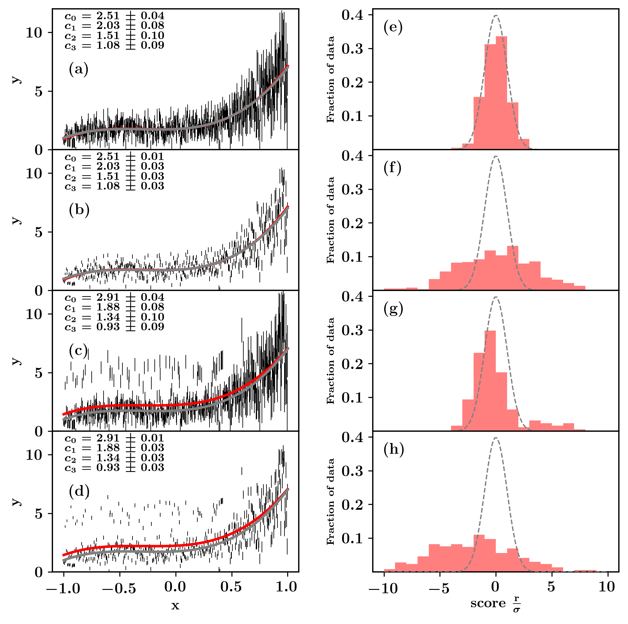
Figure 1: The four data-fitting scenarios for the toy model discussed in the text are compared. Panel (a) shows a fit to data with accurate uncertainty estimates and no outliers. Panel (b) shows a fit to data with underestimated uncertainties and no outliers. Panel (c) shows a fit to data with accurate uncertainty estimates but with outliers. Panel (d) shows a fit using data with both underestimated uncertainties and with outliers. The simulated data used for fitting are shown as black bars, the “true” underlying function used to generate the data is shown as a gray line, and the fit to the “experimental” data is shown in red. In panels (e) to (h), the normalized residuals for data in the corresponding plots are histogrammed. A normal distribution with $\mu=0$ and $\sigma^{2}=1$ (gray dashed line) is shown for reference.

So far, we have described a simple, generic inference problem and its solution. We now consider four possible scenarios for solving this problem, each involving a different possible distribution for $\bm{y}$ and $\bm{\delta_{y}}$. These differing distributions are plotted in panels (a) to (d) of Fig. 1, and defined according to:

$$\begin{split}y_{i}&\sim\mathcal{N}(T(x_{i}),0.32^{2})\\ {\delta_{y}}_{i}&=0.32T(x_{i})\\ \end{split}$$ (4)

$$\begin{split}y_{i}&\sim\mathcal{N}(T(x_{i}),0.32^{2})\\ {\delta_{y}}_{i}&=0.10T(x_{i})\\ \end{split}$$ (5)

$$\begin{split}y_{i}&\sim\mathcal{N}(T(x_{i}),0.32^{2})+\alpha\\ {\delta_{y}}_{i}&=0.32T(x_{i})\\ \end{split}$$ (6)

$$\begin{split}y_{i}&\sim\mathcal{N}(T(x_{i}),0.32^{2})+\alpha\\ {\delta_{y}}_{i}&=0.10T(x_{i}),\end{split}$$ (7)

for each $i$, where

$$\alpha\begin{cases}\sim\mathcal{N}(3,0.6^{2}),&\text{ 10\% probability},\\ =0,&\text{ 90\% probability}.\end{cases}$$

In this notation, $\sim\mathcal{N}(\mu,\sigma^{2})$ refers to sampling from a normal distribution of mean $\mu$ and variance $\sigma^{2}$.

We begin with the first scenario, shown in panel (a) of 1. This is the best-case scenario, given the assumptions appropriate for weighted-least-squares: our measuring device suffers from zero bias and the true mean measurement uncertainties $\bm{\delta_{y}}$ are known (Eq. 4). For example, our measuring device exhibits independent statistical and systematic uncertainties of $10\%$ and $30\%$, yielding a total $32\%$ total uncertainty via addition in quadrature. Because both the measured data and their uncertainties are faithful to the true underlying distribution, our estimated $\bm{\theta_{opt}}$ match $\bm{\theta_{true}}$, up to the estimated uncertainty of $\bm{\theta_{opt}}$. Panel (e) shows that the distribution of standardized residuals between our model’s predictions and the corresponding experimental data are distributed according to a normal distribution with unit variance.

Panel (b) of Fig. 1 shows the outcome of the second scenario: our measuring device performs identically as in the first scenario, but now our estimates of $\bm{\delta_{y}}$ are too small (Eq. 5). This could arise if, for instance, both statistical and systematic uncertainty contribute to the overall uncertainty of our measuring device, but we have only recognized and reported the statistical uncertainty. Because the minimum of our weighted-least-squares likelihood function is not affected by overall rescalings of $\bm{\delta_{y}}$, we recover the same $\bm{\theta_{opt}}$ as in the first scenario. However, our uncertainty estimates of $\bm{\theta_{opt}}$ have shrunk by a factor of three — the same factor by which we underestimated the measurement uncertainty – because the Hessian $\mathcal{H}(\bm{\theta_{opt}})$ scales proportionally with $\bm{\delta_{y}}$. Panel (f) shows that while the standardized residuals remain normally distributed with a mean of zero, they are more dispersed than the reference distribution. Thus, underestimation of experimental uncertainties directly causes underestimation of parametric uncertainties. This is a generic feature of parameter inference and, as we will show in the following section, affects most previous OMP analyses.

Panel (c) of Fig. 1 presents a third scenario: as in the first scenario, we have accurately estimated the experimental uncertainty $\delta$, but now our experimental device occasionally returns anomalous measurements (so-called “outliers”). The simulated data $\bm{y}$ have been drawn according to 6: each measurement has a 10% chance of being shifted upward by $\alpha$, which is an artificial “outlier factor”. This is meant to represent a more realistic situation in which some fraction of experimental data are inconsistent with the model, either because of model defects or because of problems during experimental data collection. The outliers “pull” on the likelihood function, causing our recovered $\bm{\theta_{opt}}$ to differ from those of the previous scenarios, but, because our $\bm{\delta_{y}}$ are the same as in the first scenario, our uncertainty estimates of $\bm{\theta_{opt}}$ do not change. The parameter bias appears in panel (g) as asymmetry in the standardized residuals with respect to the reference distribution, even as the variance of the residuals is the same as in the first scenario. We note that even if our measuring device returned no outliers, if our underlying model was incorrect (i.e., model defect), certain data would appear to be outliers, and we would obtain a similar result.

Finally, panel (d) of Fig. 1 combines the second and third scenarios: $\bm{y}$ contains occasional outliers and $\bm{\delta_{y}}$ are overconfident (Eq. 7). Accordingly, our estimated $\bm{\theta_{opt}}$ is biased and our uncertainty estimates of $\bm{\theta_{opt}}$ are overconfident about the biased estimates. Both the bias and the dispersion of the normalized residuals are visible in panel (h). This scenario is the best analog to the OMP optimization task. For us to obtain well-calibrated uncertainties that span the experimental data, our loss function and optimization strategy must address both challenges: namely, underestimation of experimental (co)variances, and fundamental discrepancies between the model and data either due to model defects or problems with experimental data collection (which we do not attempt to disentangle).

II.3 Challenges for CH89 and KD

The difficulties of using weighted-least-squares estimators are well-known to OMP designers, including those of CH89 and KD. A common symptom is that initial fits to experimental data are often grossly unsatisfactory, clearly missing “the physics” present in the scattering data, leading to manual parameter adjustment. The authors of CH89 comment that, early in their analysis, there were often “significant contributions from the data that the model is not able to describe” even when training to a single scattering data set. They tested several alternative loss functions but found that in “reduc[ing] the emphasis of outlying points” they “lost sensitivity to even the good data”. After testing various functions, their compromise was to introduce a weight factor to their likelihood function for each data set $s$, equal to the minimum loss for that data set obtained in a fit to only that data set, i.e.,

$$L(\bm{y}|\bm{x,\delta_{y},\theta})=\sum_{s}\frac{L_{s}(\bm{\theta}|\bm{x_{s}},\bm{y_{s}})}{min(L_{s}^{loc}(\bm{\theta}|\bm{x_{s}},\bm{y_{s}}))},$$ (8)

where $L_{s}$ is the contribution from data set $s$ to the overall weighted-least-squares fit as in Eq. 2. By deemphasizing data sets that were poor matches to the form of their OMP, they achieved a better visual fit to their training data. However, this solution also introduces problems: the introduced weights are not easily interpreted nor do they preserve the normalization of the likelihood function, which is important for estimating $\bm{\Sigma}$. However, because finding $\bm{\theta_{opt}}$ is insensitive to overall rescalings of $L$, most past authors have been willing to sacrifice the possibility of accurately estimating $\bm{\Sigma}$ in order to improve their single “best-fit” parameter vector.

Koning and Delaroche identified this issue in their global OMP characterization as well and also provided extensive quantitative evidence that traditional OMPs are incapable of reproducing the bulk of experimental data within the range of reported experimental uncertainties. In Table 12 of their OMP analysis Koning and Delaroche (2003), they present sums of uncertainty-weighted square residuals per degree of freedom (a reduced-$\chi^{2}$ metric) for several prominent OMPs against a variety of experimental data sets. In their analysis, a value near unity was taken as an indication of good model-data agreement. For the widely used global OMPs they considered, they found values of $\chi^{2}/N$ ranging from 6.3 to 11.2 for differential elastic scattering cross sections and from 2.3 to 9.2 for neutron total cross sections. Using their new potential (KD), they found values of $\chi^{2}/N$ ranging from 4.5 to 7.4 for differential elastic scattering cross sections and from 1.2 to 6.7 for neutron total cross sections, depending on the experimental data corpus tested against. They echoed the comments of the CH89 authors, noting that “the optimization procedure is very sensitive” to underestimations in reported experimental uncertainties such that “even a slightly incorrect error estimation can easily vitiate an automated fitting procedure”. In Koning (2015), Koning further analyzed model-experiment discrepancies across the EXFOR database and combined several proposed remedies into an “evaluated” $\chi^{2}$ expression meant to overcome the issues of using naïve weighted least squares.

To better understand these discrepancies between the trained model and training data, we began by reproducing the original CH89 and KD analyses. Figure 2 summarizes the performance of the standard CH89 and KD potentials against the experimental data used to train them, as reconstructed in the present work. For each experimental datum, the normalized residual for that datum ($r/\delta_{y}$) was tabulated, then all residuals histogrammed according to data type. In addition, in panel (b), two dotted curves show the performance of CH89 when the CH89 parameters are resampled according to the parameter covariance matrix presented in the original publication. If the assumptions underpinning weighed-least-squares were fulfilled, each line should follow the gray dashed line (a normal distribution with unit variance), indicating that the CH89 and KD predictions match the mean of the experimental data used to train them, and that the training data are dispersed about the predictions in keeping with their reported uncertainties. In reality, all types of scattering data show a variance several times larger than unity, an indication either of underestimation of experimentally reported uncertainties or of significant model deficiencies, or both. The means of the distributions are offset to varying degree, indicating that the canonical $\bm{\theta_{opt}}$ for these OMPs retain some bias with respect to the underlying experimental data. Table 1 lists the mean, standard deviation, and skewness of these observed distributions for each data type used to train the CH89 and KD OMPs. This confirms the issues identified by past authors: clearly, these OMPs do not span the variance of their training data, and for some data types, predictions show systematic bias with respect to experiment.

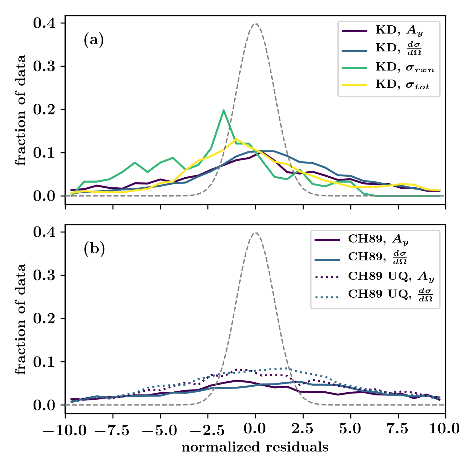
Figure 2: The distribution of normalized residuals ($r$/$\delta_{y}$) between the original CH89 and KD OMPs and their training data as reconstructed in this work are shown in panels (a) and (b), respectively. Residuals are histogrammed by data type, with all available proton and neutron data for that data type included (in contrast with Table 1 which discriminates by projectile). The curves labeled CH89 UQ refer to the UQ assessment of the original CH89 work, which we have sampled here as $\bm{\theta}\sim\mathcal{N}(\bm{\theta}_{CH89},\bm{\Sigma}_{CH89})$, where $\bm{\theta}_{CH89}$ is the canonical CH89 “best fit” parameter vector, and $\bm{\Sigma}_{CH89}$ is the canonical CH89 covariance matrix published in the original treatment.

Table 1: Mean ($\mu_{1}$), standard deviation ($\mu_{2}$), and skewness ($\mu_{3}$) for the distribution of standardized residuals between the original KD and CH89 OMPs and their training data, as reconstructed in this work. Results are tabulated separately for protons and neutrons. The columns labeled CH89 UQ refer to the UQ assessment of the original CH89 work, which we have sampled here as $\bm{\theta}\sim\mathcal{N}(\bm{\theta}_{CH89},\bm{\Sigma}_{CH89})$, where $\bm{\theta}_{CH89}$ is the canonical CH89 “best fit” parameter vector, and $\bm{\Sigma}_{CH89}$ is the canonical CH89 covariance matrix estimate published in the original treatment.

	Proton data
	CH89		CH89 UQ		KD
	$\frac{d\sigma}{d\Omega}$	$A_{y}$	$\frac{d\sigma}{d\Omega}$	$A_{y}$	$\frac{d\sigma}{d\Omega}$	$A_{y}$	$\sigma_{rxn}$
$\mu_{1}$	0.5	-3.2	1.1	0.7	0.7	-0.4	-2.4
$\mu_{2}$	29.8	30.7	9.6	7.0	18.6	18.4	3.7
$\mu_{3}$	-2.1	-3.2	-1.6	0.6	-1.0	-3.3	-1.0

	Neutron data
	CH89		CH89 UQ		KD
	$\frac{d\sigma}{d\Omega}$	$A_{y}$	$\frac{d\sigma}{d\Omega}$	$A_{y}$	$\frac{d\sigma}{d\Omega}$	$A_{y}$	$\sigma_{tot}$
$\mu_{1}$	-1.9	1.4	-1.7	1.2	-2.1	0.8	-0.3
$\mu_{2}$	5.0	6.5	4.0	4.4	4.8	6.8	25.2
$\mu_{3}$	-0.7	0.5	-0.8	0.3	-0.7	-19.9	-17.5

The comparison of these canonical OMPs with their training data led us to investigate the self-consistency of the training data themselves. We discovered that these training data sets were often inconsistent, in the sense that no plausible model could simultaneously fit them. This implies that for data routinely used in OMP training, the reported experimental uncertainties may be significantly underestimated. Figure 3 illustrates the problem: in panel (a), five independent, representative elastic scattering data sets for neutrons on ⁴⁰Ca at $14\pm 0.1$  from the EXFOR database Experimental Nuclear Reaction Data () (EXFOR) are shown. Each is comparable to the elastic scattering data sets used to train the KD and CH89 OMPs. To facilitate comparison between these data sets, which were measured at different angles, we describe their mean behavior as:

$$f(\theta)=\sum\limits_{n=0}^{10}c_{n}p_{n}(\theta)$$ (9)

where $p_{n}(x)$ are Legendre polynomials. A simple weighted-least-squares fit was performed to optimize the polynomial coefficients $c_{n}$. When the fit and training data are compared, the normalized residuals are inconsistent with one another at the several-$\sigma$ level, as shown in panel (b) of the same figure, due to underestimation of experimental uncertainties. Considering that these data were all collected for the same projectile-target system and at the same energy but are inconsistent at the several-$\sigma$ level, even larger discrepancies may be expected when comparing many types of scattering observables on different nuclei and energies during global OMP parameter inference. (It is worth mentioning that, of the data types considered for training OMPs, such experimental uncertainty underestimation appears to be most acute for differential elastic scattering data.) To be reliable, any data-driven assessment of OMP uncertainty must address this unaccounted-for dispersion of the experimental data. Moreover, if we can determine how large such unaccounted-for uncertainty must be to bring the optimized OMP and experimental data into agreement, we gain insight into the degree of mutual consistency between the OMP and the data libraries used to train the OMP.

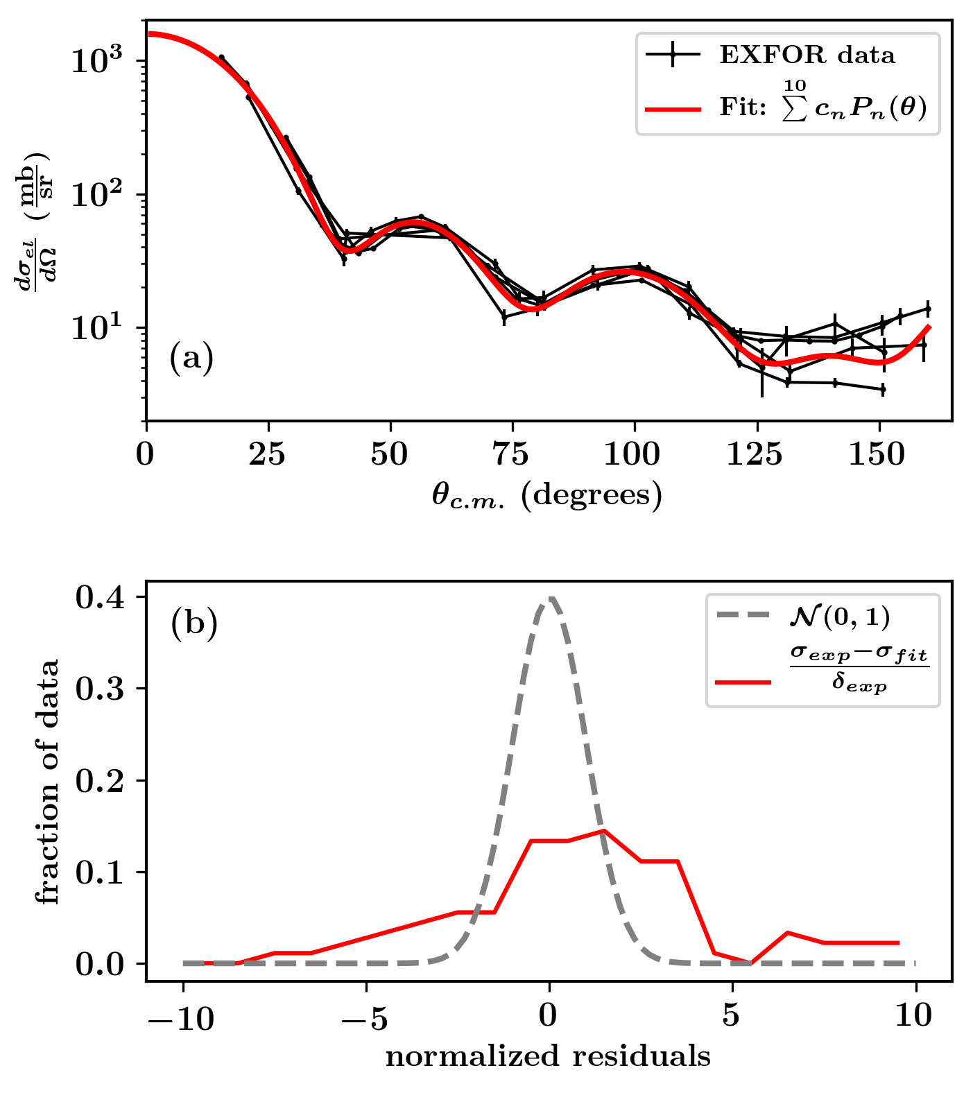
Figure 3: Five experimental data sets for ⁴⁰Ca(n,n)⁴⁰Ca at 14  show significant variability, despite being collected under similar kinematic conditions. In panel (a), each data set is shown as a series of black points with the reported experimental uncertainties. A weighted-least-squares fit of all points, using the sum of the first ten Legendre polynomials as a model, is shown in gray. Panel (b) shows the normalized residuals for the experimental data points as a histogram (red line). A Gaussian distribution with unit variance is shown for reference (gray dashed line).

III Improved inference for OMPs

In this section, we present our implementation for improved OMP parameter inference. We propose a modified likelihood function that addresses the problems of canonical OMP analysis as identified in the previous section. We then describe our implementation of the CH89 and KD OMPs, our scattering code, and the MCMC tools we used for performing parameter inference.

III.1 Likelihood function

For a training corpus consisting of $N$ experimental data, denoted ($\bm{x,y,\delta_{y}}$), and an OMP with $k$ free parameters $\bm{\theta}$, we define our likelihood function as follows:

$$\begin{split}L(\bm{y}|\bm{x,\delta_{y},\theta,\delta_{u}})&=\frac{1}{\sqrt{(2\pi)^{k}|\bm{\tilde{\Sigma}}|}}e^{-\frac{1}{2}\bm{r}^{\intercal}\bm{\tilde{\Sigma}}^{-1}\bm{r}},\\ \bm{r}&\equiv\bm{y}-M(\bm{\theta},\bm{x}).\end{split}$$ (10)

In place of the true (unknown) data covariance matrix $\bm{\Sigma}$, we have introduced a diagonal covariance matrix ansatz $\bm{\tilde{\Sigma}}$:

$$\bm{\tilde{\Sigma}}\equiv\frac{k}{N}\begin{bmatrix}\Delta_{1}&&\\ &\ddots&\\ &&\Delta_{N}\\ \end{bmatrix};\Delta_{1,\ldots,N}\in\bm{\Delta}.$$ (11)

In this prescription, the augmented variances $\bm{\Delta}$ combine the experimentally reported uncertainties $\bm{\delta_{y}}$ with an new unaccounted-for uncertainty for each datum, $\bm{\delta_{u}}$:

$$\bm{\Delta}=\{(\delta_{y}^{2}+\delta_{u}^{2}):\delta_{y}\in\bm{\delta_{y}},\delta_{u}\in\bm{\delta_{u}}\},$$ (12)

where each $\delta_{u}$ is calculated as follows:

$$\bm{\delta_{u}}=\{\frac{y+M(\bm{\theta},x)}{2}\times\delta_{t}:x\in\bm{x},y\in\bm{y},\delta_{t}\in\bm{\delta_{T=\hat{t}(y)}}\}.$$ (13)

To clarify these expressions, we start with the terms in Eq. 13. As discussed in the previous section, the reported uncertainties for experimental measurements are often too small to be self-consistent, hindering robust OMP UQ assessment. As such, we need a way of increasing our uncertainty in the experimental data that is consistent with the expectation that different types of experimental data (differential elastic cross sections, neutron total cross sections) will have different degrees of uncertainty underestimation. At the same time, we want to respect the reported experimental uncertainty, as it represents the measurer’s informed judgement about uncertainty affecting the measurement, even if in aggregate, they are often underestimated. Our solution is to create a random variable $\delta_{T}$, representing unaccounted-for uncertainty, for each type of experimental data appearing in the training corpus. For example, in the CHUQ training corpus, there are four types of experimental data: differential elastic scattering cross sections and analyzing powers, each for protons and neutrons. As such, we create four random variables, each representing some degree of unaccounted-for uncertainty for measured data of that type. At present, we do not know the value of these random variables $\bm{\delta_{T}}$, so we treat them as parameters to be learned alongside the OMP parameters $\bm{\theta}$.

Returning to Eq. 13, for each experimental datum in the training set, we calculate a datum-specific unaccounted-for uncertainty term $\delta_{u}$, which is the product of the average of the model prediction $M(\bm{\theta},x)$ and the experimental datum value $y$ with the unaccounted-for uncertainty $\delta_{T}$ of that datum’s data type. (The term $\bm{\delta_{T=\hat{t}(y)}}$ should be read as “a $N$-long vector of $\delta_{T}$ values, each corresponding to the data type of experimental measurement $y$”.) Thus for each datum of the same type, the individual unaccounted-for uncertainty $\delta_{u}$ is calculated using the same $\delta_{T}$.

With $\bm{\delta_{u}}$ defined, we proceed to Eq. 12. For each experimental training datum, the reported uncertainty $\delta_{y}$ is added in quadrature with that datum’s $\delta_{u}$ yielding the overall uncertainty $\Delta$ for that training datum. The vector of these augmented uncertainties, $\bm{\Delta}$, enters Eq. 11, which defines the covariance matrix ansatz. The entries of $\bm{\tilde{\Sigma}}$ are scaled by $k/N$ in recognition that, by replacing the $k\times k$-matrix $\bm{\Sigma}$ with an $N\times N$ covariance matrix ansatz $\bm{\tilde{\Sigma}}$, a scaling factor is required to approximately preserve the matrix determinant that features in the overall normalization. This is equivalent to saying that the $N$ training data cannot all be independent random variables, as the information they contain can span, most, the $k$ dimensions of $\bm{\theta}$.

In sum, our likelihood function (Eq. 10) replaces the unknown covariance matrix $\bm{\Sigma}$ with a diagonal matrix of variance terms $\bm{\Delta}$, each of which has been augmented based on the unaccounted-for-uncertainty $\delta_{T}$ for each data type. If reasonable values can be learned for unaccounted-for uncertainties $\bm{\delta_{T}}$ in tandem with $\bm{\theta}$, this approach will yield both a fitted OMP with good coverage of the training data and also a sense of the missing uncertainty required to bring the experimental data into agreement with the model. We remain agnostic about about the source of the unaccounted-for uncertainty, be it underestimation of experimental uncertainty, model deficiencies, errors in the tabulation of experimental results, insufficient numerical precision during model calculations, or an “unknown unknown”. The practical effect of each $\Delta$ is the same as in traditional weighted-least-squares, namely, to reduce the contribution of residuals to the overall likelihood.

If we place the likelihood function in the the log-likelihood form relevant for optimization,

$$\log{L(\bm{y}|\bm{x,\delta_{y},\theta,\delta_{T}})}=-\frac{1}{2}\left[\frac{\bm{r^{T}r}}{|\bm{\tilde{\Sigma}}|}+\log{|\bm{\tilde{\Sigma}}|}+k\log{(2\pi)}\right].$$ (14)

it becomes clear that minimizing the log-likelihood involves a competition between the first and second terms inside the brackets. Larger $\bm{\delta_{T}}$ values make for larger $\bm{\Delta}$ and a larger covariance determinant $|\bm{\tilde{\Sigma}}|$, which reduces the first term but increases the second term. At the optimum, where $\bm{\theta}$ minimizes the contribution from residuals, both terms should be equal,

$$\bm{r^{T}r}=|\bm{\tilde{\Sigma}}|\log{|\bm{\tilde{\Sigma}}}|.$$ (15)

This implies that, at the start of training our OMP, our unaccounted-for uncertainty random variables $\bm{\delta_{T}}$ will grow rapidly, to counterbalance the large residuals between model and data, but, as the fit improves and the residuals shrink, $\bm{\delta_{T}}$ will grow smaller.

We note that the factor $k/N$ in the covariance ansatz is the simplest but not the only choice to account for the unknown degree of correlation between individual data. For example, one might expect a priori that experimental data of each type (such as proton reaction cross section, neutron analyzing powers, etc.) will correlate strongly with each other, due to common features of the experimental design or ease of certain types of measurement, but correlate more weakly with data of other data types. Accordingly, one might want to ensure that each data type contributes equally to the overall likelihood, independent of how many data points it contains, so that data types with fewer data points are not outvoted by data types with better experimental coverage. In that case, $\bm{\tilde{\Sigma}}$ could be modified to be:

$$\bm{\tilde{\Sigma}}\equiv\frac{k}{n_{t}}\begin{bmatrix}\frac{1}{N_{1}}\Delta_{1}\\ \vdots\\ \frac{1}{N_{1}}\Delta_{N_{1}}\\ \frac{1}{N_{2}}\Delta_{N_{1}+1}\\ \vdots\\ \frac{1}{N_{2}}\Delta_{N_{1}+N_{2}}\\ \frac{1}{N_{3}}\Delta_{N_{1}+N_{2}+N_{3}}\\ \vdots\\ \frac{1}{N_{T}}\Delta_{N}\\ \end{bmatrix}\times I_{N}$$ (16)

where $n_{t}$ is the number of unique data types $t$, and $N_{t}$ is the number of data points of type $t$, and $I_{N}$ is the identity matrix of dimension $N$. With this choice for $\bm{\tilde{\Sigma}}$, all data points of a given data type would be given equal influence for that type, and each data type would be given equal influence on the overall likelihood. Any additional information about the covariance structure of the experimental data, such as knowledge of the systematic error for one or more specific data sets, can be directly inserted to turn $\bm{\tilde{\Sigma}}$ into a more-realistic block-diagonal matrix. We experimented with a handful of alternatives, including Eq. 16, and found that their impact on the final uncertainty-quantified OMPs was small except in situations where one training data type had far fewer data points than the other types (see Fig. 13 in Section IV.3). Unless noted otherwise, all results in the following sections were generated using Eq. 10 as the likelihood function.

Finally, as discussed in toy-model scenarios two and four of Section II.2, we still need a way of identifying outliers in the training data corpora. By outlier, we mean a datum that should not be used to train the model, either because the model is missing physics that the data capture (e.g., effects of deformation if the model assumes sphericity), or because the data are erroneous. In either of these cases, training the model to the datum would bias model parameters. To identify outliers, we implemented a procedure similar to that by Pérez, Amaro, and Arriola in their analysis of the NN interaction via partial wave analysis of NN scattering data Pérez et al. (2013), and first suggested by Gross and Stadler Gross and Stadler (2008). Briefly, in a standard NN scattering database they examined, they found that certain data collected in similar kinematic conditions were mutually inconsistent up to the experimentally reported uncertainties. Rather than reject all inconsistent data as outliers, they used an iterative procedure to simultaneously train a model to these data while updating the outlier status of each datum used for training. In the initial step, their model was fit to the full corpus of NN-scattering data. Any data lying $>3\sigma$ away from the model, where $\sigma$ was taken to be the reported experimental uncertainty, were flagged as outliers and not included in the following round of fitting. In the second round, the model was fitted to the smaller set of “inlier” data, then the outlier status of each datum was assessed again, based on the second fit. The process was repeated until the model fit and the outlier status of each data point became stable, yielding a mutually-consistent database, up to the fitted model. Certain data that were initially incompatible with the others were thus recovered as the model fit improved over multiple iterations.

Our procedure was the same except in two respects. In our case, for $\sigma$ we included both the variance of the model prediction from MCMC and the experimental uncertainty, summed in quadrature:

$$\bm{\sigma}^{2}=\{\delta_{y}^{2}+var[M(\bm{\theta},x)]:\delta_{y}\in\bm{\delta_{y}},x\in\bm{x}\}$$ (17)

Second, because MCMC involves sampling noise, many walker steps are often required before walkers have time to react to changes in the outlier status of the experimental data. Thus, we updated the outlier status of the training data only at 100-step intervals during MCMC, rather than at every step.

III.2 CH89 and KD implementation

We turn now to the implementation of the OMPs we retrained according to our proposed approach. Both the CH89 and KD OMPs assume a spherical optical potential, smooth in scattering energy $E_{lab}$ and target $A$, for modeling the projectile-target interaction. CH89 Varner et al. (1991) was restricted to proton and neutron elastic scattering cross sections and analyzing powers on nuclei “in the valley of stability” with $40\leq A\leq 209$ and for scattering energies of $10\leq E\leq 65$  (assumed to be the lab frame). The potential consists of five terms: a real central potential, an imaginary central potential, an imaginary surface potential, a real spin-orbit potential, and for protons, a Coulomb potential (see the Appendix for detailed functional forms). In all, these components employ 22 free parameters. To perform comparisons with experimental data, the authors of CH89 used a joint scattering-optimization code called MINOPT, a hybrid of the scattering code OPTICS Eastgate et al. (1973) and the CERN optimization code MINUIT James and Roos (1975). For the wave equation, the original treatment used the non-relativistic Schrödinger equation. Because the lowest considered scattering data energy was $10$ , the original treatment took the compound-nucleus contribution to be zero.

The KD global OMP Koning and Delaroche (2003) was fitted not only to proton and neutron elastic scattering cross sections and analyzing powers, but also to proton reaction (or “non-elastic”) and neutron total cross sections. The authors define its domain as “(near)-spherical” nuclei with $24\leq A\leq 209$ for incident scattering energies of $0.001\leq E\leq 200$  in the lab frame. In addition to the potential component types used in CH89, KD adds an imaginary spin-orbit component. Each component was made substantially more flexible in energy- and asymmetry-dependence, bringing the total number of free parameters to 46. To perform comparisons with experimental data, the developers used the scattering code ECIS-97, as accessed through a visual interface called ECISVIEW. For the wave equation, the authors “[employed] the relativistic Schrödinger equation throughout”, using “the true masses of the projectile and target expressed in atomic mass units”. To manage optimization in this higher-dimensional space, they developed a new approach they called “computational steering”: a user manually adjusted parameters in real time to achieve a good visual fit, which was followed by an automated simulated annealing procedure using the program SIMANN to achieve a quantitative optimum.

For our recharacterization of these OMPs, we adhered to the original potential forms and scattering assumptions as described above but with a few minor differences. First, scattering calculations for CH89 were performed according to the same relativistic-equivalent Schrödinger equation used for KD calculations rather than the non-relativistic treatment of the original. The effect was to slightly improve the fidelity of calculated cross sections at the highest scattering energies included in the CHUQ corpus (65 MeV). Second, for differential elastic scattering cross sections at scattering energies below roughly 10-15   the elastic contribution from the compound nucleus becomes significant compared to the direct contribution from the OMP and must be included for comparison to experimental data. The authors of CH89 restricted their data corpus to scattering energies $\geq 10$ for this reason. For the KDUQ corpus, however, roughly 10% of the elastic scattering data were collected below $10$ . To enable comparison with these data, Koning and Delaroche used the compound cross section values generated by ECIS-97, the same code they used for direct scattering calculations. In our case, we generated compound elastic cross sections using the LLNL Hauser-Feshbach code YAHFC Ormand , using the canonical parameters of KD to generate the transmission coefficients needed for the calculation.

III.3 Scattering code and MCMC

For scattering calculations and parameter inference, we combined the MCMC utility emcee Foreman-Mackey et al. (2013) with a new, lightweight C++ and Python library, tomfool, that we developed to perform single-nucleon scattering calculations. Cross sections were generated via a calculable-$R$-matrix Lagrange-mesh method after Descouvement and Baye (2010); Baye (2015) detailed in the Appendix. The use of a Lagrange-Legendre basis instead of a radial basis accelerates calculations severalfold but at the cost of a small loss of precision, depending on the number of basis elements and chosen $R$-matrix channel radius. To ensure fair comparison with the original CH89 and KD analyses, we applied several measures to validate our calculation pipeline. First, wherever possible, we drew mathematical functions from the Gnu Scientific Library (GSL) Galassi, M. et al. . Any necessary functions unavailable in GSL (such as optical potential functional forms and relativistic kinematics equations) were subjected to a suite of unit and integration tests, including comparison against results from the well-tested scattering code frescox Thompson (1988, ) and lise++ Tarasov and Bazin (2016); Tarasov . For relativistic calculations, in addition to treating scattering energies and angles relativistically, we use the wavenumber and optical-potential rescaling approximations given by Eqs. 17 and 20/21 of Ingemarsson (1974), the same formulae used for this purpose in frescox and talys. Using frescox we prepared a set of cross section benchmarks covering a range of scattering energies, angles and targets representative of the KDUQ corpus. Using an $N=30$ Lagrange-Legendre basis, an $R$-matrix channel radius of 15 f , a maximum partial wave angular momentum $l_{max}=80$, and a convergence threshold of $10^{-6}$ for the magnitude of $S$-matrix elements, we achieved agreement with the frescox benchmarks to 1% or better, both for our relativistic and non-relativistic implementations for CH89 and KD. This configuration was used for all scattering calculation results in our analysis. Finally, we performed numerous spot checks against the figures in the original CH89 and KD papers to confirm that our implementation of their OMPs generates the same cross sections to within the graphical resolution of the original publications.

For each OMP parameter, we assigned a weakly informative truncated Gaussian prior centered on the canonical parameter value (that is, centered on the parameter values from the original KD and CH89 publications). For each prior we set the variance based on our estimates about the sensitivity of scattering observables to changes in that type of parameter. For example, a change of 20% in a Woods-Saxon radius or diffuseness would result in large changes to the location of elastic scattering diffraction minima and would thus be relatively unlikely, but not impossible, given the level of consistency among the experimental data. In contrast, the energy-dependence of the depth of the imaginary spin-orbit potential is likely only very weakly sensitive to available experimental data, so a deviation by a factor of 2 or more from the canonical value in KD would not be surprising. Absolute upper and lower limits of the truncated Gaussian priors were set to prevent any single parameter from becoming non-physical, resulting in, for example, a negative radius. For the unaccounted-for uncertainty random variables $\bm{\delta_{T}}$, we assigned truncated Gaussian priors as

$$\delta_{t}\sim\mathcal{N}(\mu=0.2,\sigma=0.2;\delta_{t}>0),$$ (18)

for differential elastic observables and

$$\delta_{t}\sim\mathcal{N}(\mu=0.02,\sigma=0.02;\delta_{t}>0),$$ (19)

for integral observables $\sigma_{rxn}$ and $\sigma_{tot}$. This corresponds to an expectation of 20% unaccounted-for uncertainty in differential data types and 2% unaccounted-for uncertainty in integral data types. We based these priors on the observed degree of agreement of the canonical KD and CH89 potentials against their training corpora and on the typical range experimentally reported uncertainties for these types of data. To begin MCMC, $8\times k$ walkers were initialized according to

$$\bm{\theta},\bm{\delta_{t}}\sim\mathcal{N}(\mu=\mu_{prior},\sigma=0.1\sigma_{prior})$$ (20)

for CHUQ and

$$\bm{\theta},\bm{\delta_{t}}\sim\mathcal{N}(\mu=\mu_{prior},\sigma=0.01\sigma_{prior})$$ (21)

for KDUQ, with $k$ the number of parameters subject to inference. For the MCMC proposal distribution, we used the emcee Foreman-Mackey et al. (2013) default proposal distribution, the affine-invariant Goodman-Weare sampling prescription, but with a scaling parameter $a=1.4$, reduced from the default value of $a=2$ to improve the acceptance fraction given the high dimensionality of the parameter space. Sampling continued for roughly 10,000 samples until ensemble means no longer exhibited movement in any parameter dimension and the percentage of each data type that were flagged as outliers ceased to change (excepting $\approx 0.1\%$ fluctuations due to the Monte Carlo nature of sampling). Due to our expectation of very long autocorrelation times among walkers, we used only the terminal sample from each walker for all results shown below.

Our reassembly of the training data corpora used to train the canonical OMPs is detailed in the Supplemental Material Sup . While we were able to recompile and verify almost all of the training data as originally used, there were a handful of discrepancies between data as reported in the referenced literature, the data as listed in the canonical CH89 and KD treatments, and the data as listed in the EXFOR experimental reaction database. Details of these differences and references to the EXFOR accession number for the data set in question (or, if the data were not available through EXFOR, to the original literature) are provided in the Supplemental Material Sup . Because our approach involves outlier-rejection and unaccounted-for uncertainties that were as large or larger than experimentally reported uncertainties, the few discrepancies were unlikely to have any appreciable effect on our analysis.

IV Results

Our results are organized in three parts. First, we compare the performance of CHUQ against that of CH89 with respect to their training data. To assess predictive power, CHUQ and CH89 are compared against a Test corpus of new scattering data collected from 2003-2020 (after the publication of the original treatment). Next, we present a similar comparison for KDUQ and KD. Last, we discuss the comparative uncertainty of the potentials, including comparison of volume integrals and how alternative likelihood functions could affect our results.

IV.1 CH89 vs CHUQ performance

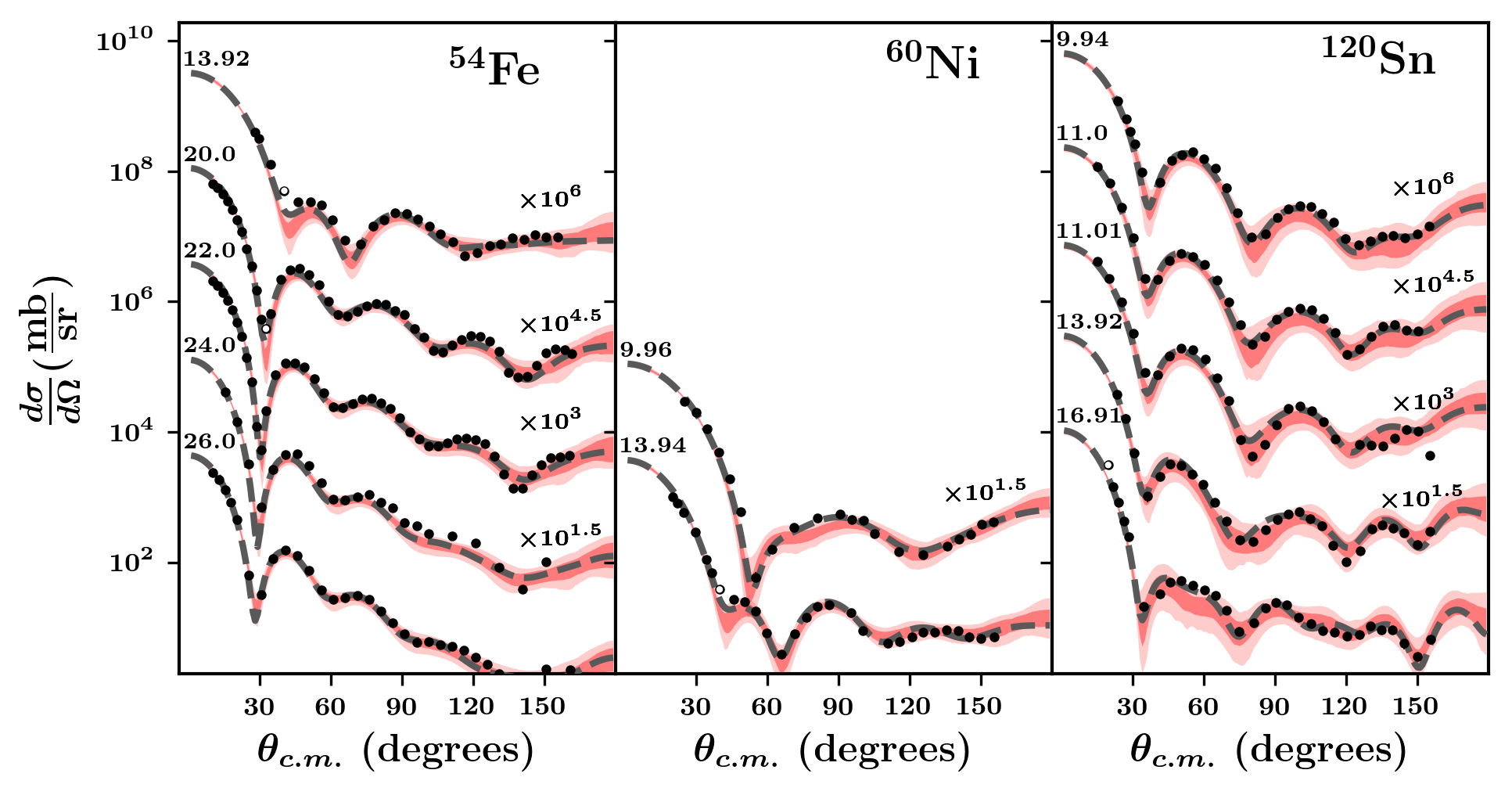
Figure 4: Representative experimental and calculated neutron differential elastic cross sections are plotted for ⁵⁴Fe, ⁶⁰Ni and ¹²⁰Sn at selected energies. Experimental data are shown as points with reported experimental uncertainties. The outlier status of each point (as defined previously) is indicated by color: black points are inliers, and white points are outliers. Calculations from the canonical CH89 parameters are shown as a gray dashed line. The CHUQ 68% and 95% uncertainty intervals are shown as dark and light red bands, respectively. The data sets are labeled by scattering energy (MeV, in the lab frame) and offset vertically for legibility.

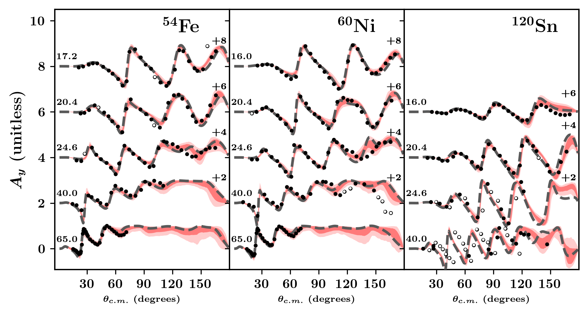
Figure 5: Representative experimental and calculated proton analyzing powers are plotted for ⁵⁴Fe, ⁶⁰Ni and ¹²⁰Sn at selected energies. See caption of Fig. 4 for key.

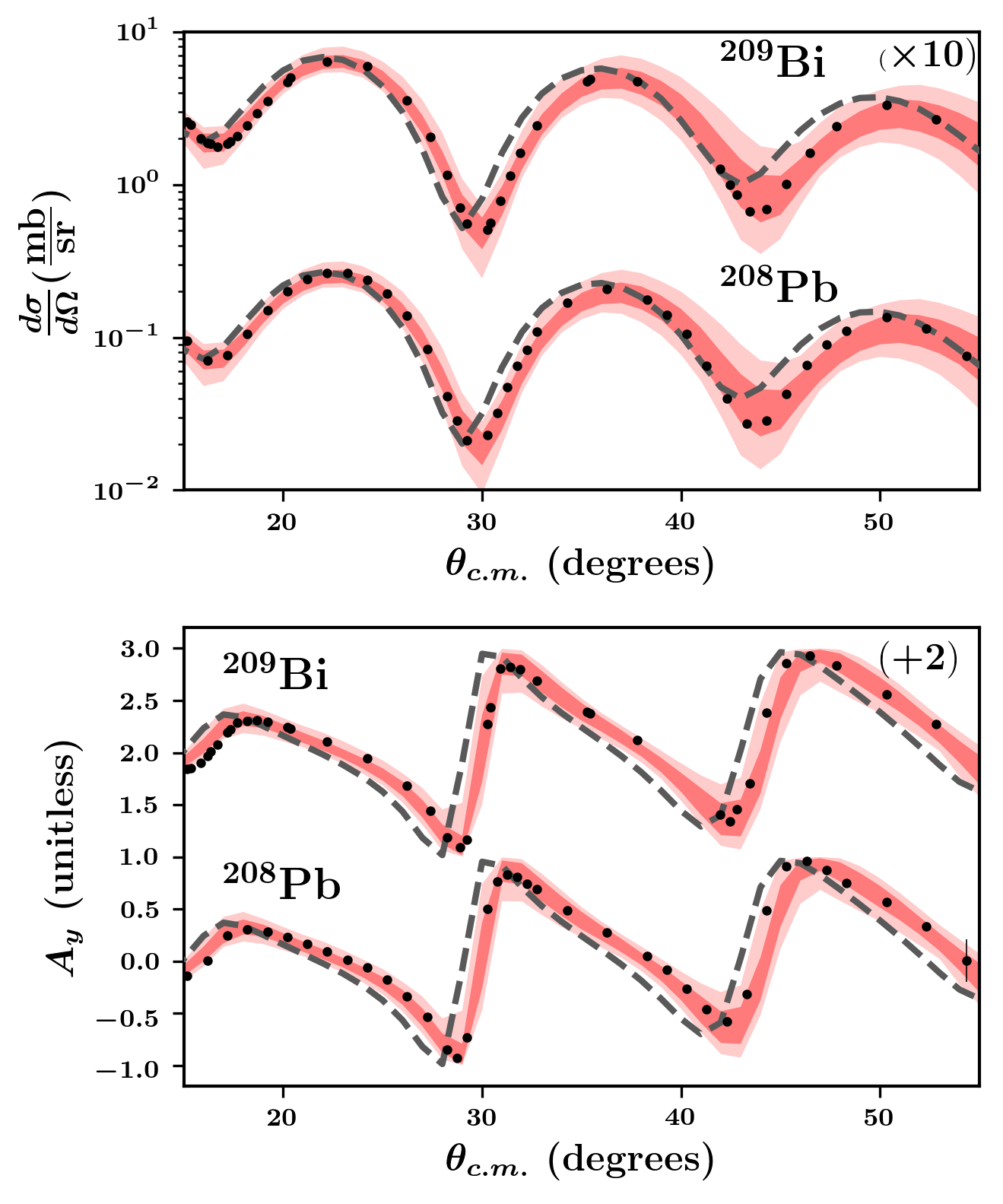
Figure 6: CH89 and CHUQ predictions are compared against experimental proton elastic scattering observables on ²⁰⁸Pb and ²⁰⁹Bi at 65 . See caption of Fig. 4 for key.

Figure 7: Normalized residuals ($r_{i}$/$\delta_{i}$) between CHUQ’s predictions and the CHUQ corpus and Test corpus are histogrammed by data type. Panel (a) shows performance against the CHUQ corpus. Panel (b) shows performance against the Test corpus.

Figures 4 and 5 show the performance of CHUQ and the canonical CH89 OMP with respect to several representative experimental data sets in the CHUQ training corpus. Figures comparing CHUQ and CH89 over the entire CHUQ corpus are provided in the Supplemental Material Sup . Overall, the median predictions of CHUQ are very similar to the canonical CH89 predictions, with the largest differences being slightly lower predicted differential elastic cross sections from CHUQ compared to those from CH89 around 10-11 , the lowest scattering energies considered in the CHUQ corpus. Compared to the canonical CH89 analysis, our use of a fully relativistic-equivalent Schrödinger equation in the present work and our relaxation of the fixed Coulomb radius parameters $r_{c}$ and $r_{c}^{(0)}$ for CHUQ improves the angular dependence of proton differential elastic scattering predictions at higher energies on high-$A$ targets, as shown in Fig. 6.

Figure 7 summarizes the overall performance of CHUQ against the full CHUQ corpus and against the Test corpus. The means, standard deviations, and skewnesses of the residual distributions shown in Fig. 7 are listed in Table 2. Using the CHUQ corpus, we can directly compare the original treatment’s uncertainty estimation (CH89 UQ in Fig. 2 and Table 1) and that of the present work (CHUQ in Fig. 7, panel (a), and Table 7). Across the data types in the CHUQ corpus, CHUQ yields similar mean residuals: between -1.0 and 1.0, versus -1.7 to 1.1 for CH89 UQ. This suggests that both the canonical CH89 parameters and CHUQ’s central parameter values do well at reproducing average trends of training data. In CHUQ, there is apparent tension between neutron differential elastic scattering cross sections, which are slightly underpredicted ($\mu_{1}=-1.0$) and proton and neutron differential elastic scattering analyzing powers, which are slightly overpredicted ($\mu_{1}=1.0$ and $\mu{1}=0.9$).

The main difference is that compared to CH89 UQ, CHUQ yields much smaller residual standard deviations: between 1.7 to 2.1 across data types, versus 4.0 to 9.6 for CH89 UQ. That the variance of the residuals is much closer to unity indicates that the larger parametric uncertainty of CHUQ more faithfully represents the spread of the experimental data in the CHUQ corpus. Further, the fact that the variance of CHUQ-corpus residuals remains larger than unity shows that the priors we assigned to the unaccounted-for uncertainties $\delta_{T}$ are preventing $\delta_{T}$ from becoming even larger, which would further reduce the constraining power of the training data.

Panel (b) of Fig. 7 illustrates performance of CHUQ against the Test corpus. The Test corpus includes many scattering data far beyond the prescribed range of validity given by the authors of CH89, including data collected at scattering energies from 1-10  and from 65-295 , proton $\sigma_{rxn}$ and neutron $\sigma_{tot}$ data, and data from targets with $A<40$. The performance of CHUQ is moderately degraded on the Test corpus compared to the CHUQ corpus, with mean residuals ranging from -1.8 to 2.0 across data types, and residual standard deviations ranging from 1.3 to 3.1 for elastic observables. Though the CHUQ corpus used for training did not include either proton $\sigma_{rxn}$ or neutron $\sigma_{tot}$ data, CHUQ’s average performance against the Test corpus in these data sectors is surprisingly good, with mean residuals of 0.3 for proton $\sigma_{rxn}$ and -0.3 for neutron $\sigma_{tot}$. This indicates that despite substantial unaccounted-for uncertainty in the training data, fits that employ only elastic scattering data can still provide meaningful constraints on the imaginary terms in the potential.

Table 2: Mean ($\mu_{1}$), standard deviation ($\mu_{2}$), and skewness ($\mu_{3}$) for the distributions of standardized residuals between CHUQ and experimental data, as shown in Fig. 7. Here the distributions are tabulated separately for protons and neutrons (cf. with Tables 3 and 1).

	Proton data
	CHUQ Corpus		Test Corpus
	$\frac{d\sigma}{d\Omega}$	$A_{y}$	$\frac{d\sigma}{d\Omega}$	$A_{y}$	$\sigma_{rxn}$
$\mu_{1}$	0.0	1.0	-0.3	-1.8	0.3
$\mu_{2}$	2.1	2.1	3.1	1.3	0.2
$\mu_{3}$	-0.1	1.6	-0.9	-2.8	0.1

	Neutron data
	CHUQ Corpus		Test Corpus
	$\frac{d\sigma}{d\Omega}$	$A_{y}$	$\frac{d\sigma}{d\Omega}$	$A_{y}$	$\sigma_{tot}$
$\mu_{1}$	-1.0	0.9	-1.2	2.0	-0.3
$\mu_{2}$	1.7	1.9	1.8	2.3	2.2
$\mu_{3}$	-0.7	0.5	-0.2	0.1	-2.1

IV.2 KD vs KDUQ performance

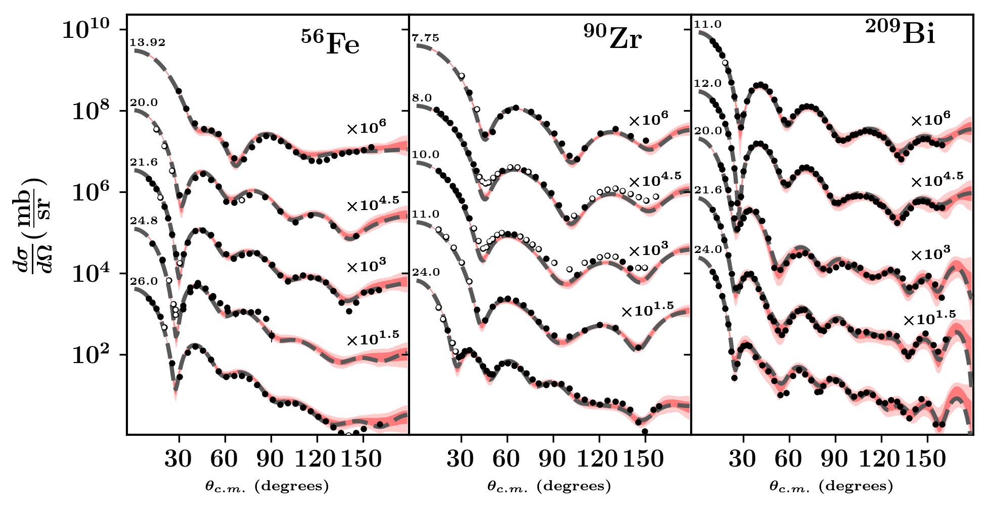
Figure 8: Representative experimental and calculated neutron differential elastic cross sections are plotted for ⁵⁶Fe, ⁹⁰Zr and ²⁰⁹Bi at selected energies. Experimental data are shown as points with associated uncertainties. The outlier status of each point (as defined previously) is indicated by color: black points are inliers, and white points are outliers. Cross sections calculated using the original KD formulation are shown via gray dashed line. The KDUQ 68% and 95% uncertainty intervals are shown as dark and light red bands, respectively. The data sets are labeled by scattering energy (MeV, in the lab frame) and offset vertically for legibility.

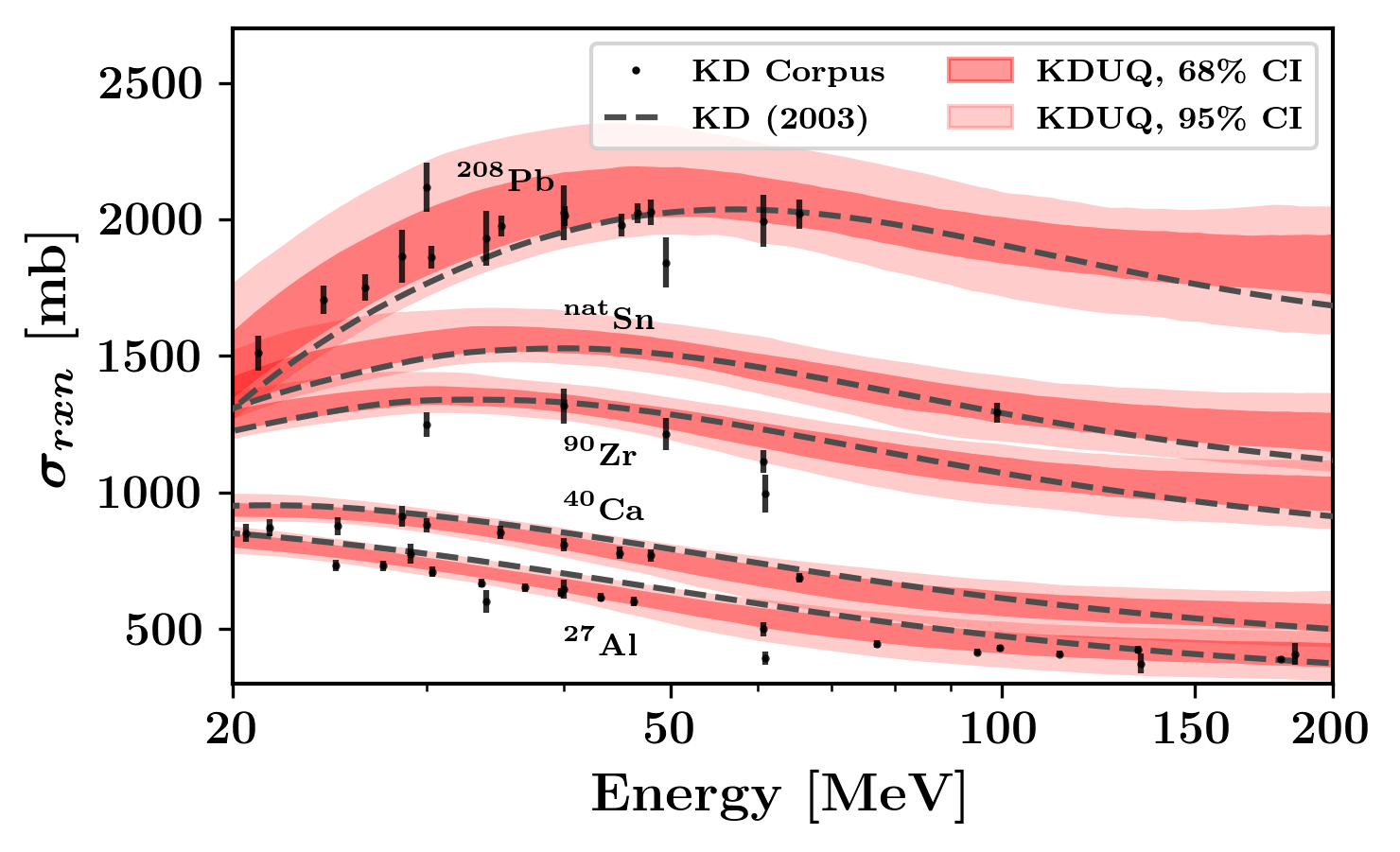
Figure 9: Representative experimental proton reaction cross section data and KD and KDUQ calculations are plotted for selected nuclei in the KDUQ corpus. See caption of Fig. 8 for additional information on the legend.

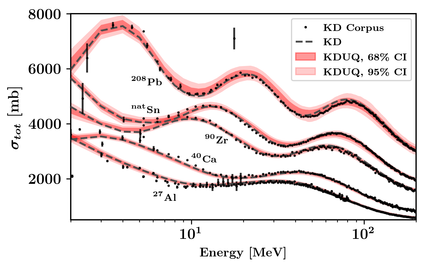
Figure 10: Representative experimental neutron total cross section data and KD and KDUQ calculations are plotted for selected nuclei in the KDUQ corpus. See caption of Fig. 8 for additional information on the legend.

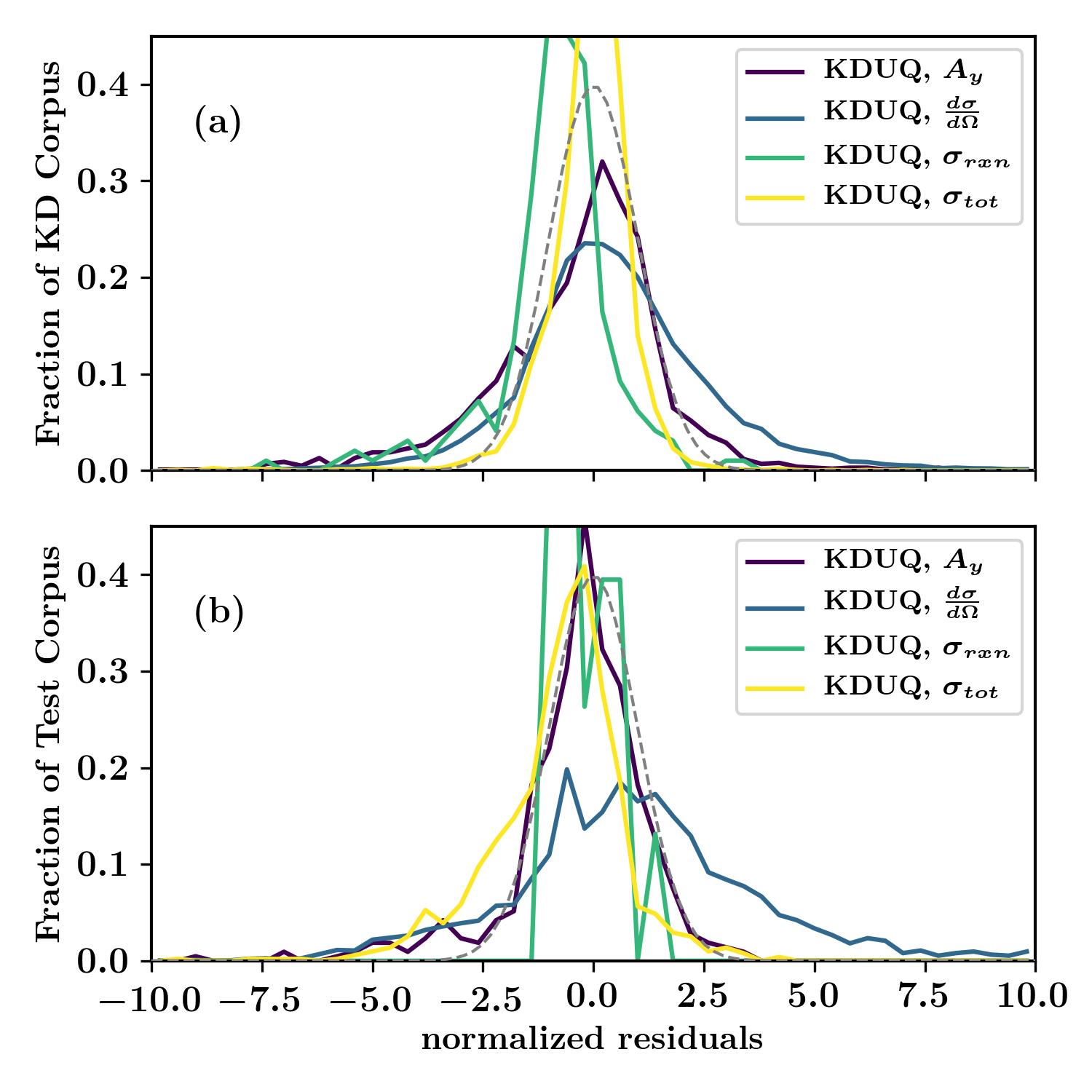
Figure 11: Normalized residuals ($r_{i}$/$\delta_{i}$) between KDUQ’s predictions and the KDUQ corpus and Test corpus are histogrammed by data type. Panel (a) shows performance against the KDUQ corpus. Panel (b) shows performance against the Test corpus.

Table 3: Mean ($\mu_{1}$), standard deviation ($\mu_{2}$), and skewness ($\mu_{3}$) for the distributions of standardized residuals shown in Fig. 11, shown separately for protons and neutrons (cf. with Tables 2 and 1).

	Proton data
	KDUQ Corpus			Test Corpus
	$\frac{d\sigma}{d\Omega}$	$A_{y}$	$\sigma_{rxn}$	$\frac{d\sigma}{d\Omega}$	$A_{y}$	$\sigma_{rxn}$
$\mu_{1}$	-0.1	0.5	-0.9	0.1	-0.8	-0.2
$\mu_{2}$	2.2	2.1	1.5	0.9	1.8	0.7
$\mu_{3}$	-0.6	1.5	-2.5	0.6	9.3	0.6

	Neutron data
	KDUQ Corpus			Test Corpus
	$\frac{d\sigma}{d\Omega}$	$A_{y}$	$\sigma_{tot}$	$\frac{d\sigma}{d\Omega}$	$A_{y}$	$\sigma_{tot}$
$\mu_{1}$	-1.1	0.5	-0.1	-1.5	1.2	-0.8
$\mu_{2}$	2.1	2.3	1.2	2.0	3.3	1.5
$\mu_{3}$	-0.6	0.3	-5.3	-0.8	1.1	-0.7

Figures 8, 9, and 10 show the performance of KDUQ and the canonical KD Global OMP with respect to several representative experimental data sets in the KDUQ corpus used for training. Figures comparing KDUQ and KD over the entire KDUQ corpus are provided in the Supplemental Material Sup . For elastic scattering observables, the median predictions of KDUQ are very similar to the canonical KD predictions at low angles, with moderate deviations appearing at higher angles and scattering energies. Predicted neutron $\sigma_{tot}$ of KDUQ and KD are nearly identical, and both achieve excellent agreement with the training data above the resolved-resonance region. (At lower energies where resonance structure is resolved, the OMP assumption of smooth, resonance-averaged behavior is no longer expected to hold). The most significant difference between KDUQ and KD is the improved reproduction of proton $\sigma_{rxn}$ cross sections in KDUQ, where predictions are roughly 10% smaller for low-$A$ targets such as ²⁷Al and ⁴⁰Ca compared to the predictions of KD. In addition, at scattering energies $>100$  across all masses, the slope of predicted proton $\sigma_{rxn}$ cross sections differs between KDUQ and KD, with KD predictions exhibiting a steeper decrease with respect to energy, whereas KDUQ predictions remain roughly flat with respect to energy. Past analyses with dispersive optical potentials have connected the energy dependence of $\sigma_{rxn}$ cross sections in this region with the behavior of deeply bound, highly correlated nucleons, as probed in (e,e’p) reactions Atkinson and Dickhoff (2019), and potentially correlated with neutron skins in neutron-rich nuclei Atkinson et al. (2020); Pruitt et al. (2020b). Such a relationship could be quantitatively assessed with a global dispersive OMP (à la Morillon and Romain (2006)), but treated fully non-locally to maintain good particle number and equipped with UQ as shown here.

Figure 11 summarizes the performance of KDUQ against both the KDUQ corpus training data and the Test corpus. The mean, standard deviation, and skewness of the distribution of residuals shown in Fig. 11 are listed in Table 3 for both protons and neutrons. Overall, KDUQ performance differs little between the KDUQ corpus and Test corpus, an indication that our MCMC-based approach has avoided overfitting the training data. Compared to KD, KDUQ has a lower bias with respect to proton reaction cross section data (mean normalized residual of -0.9; cf. with -2.4 for KD in Table 1). Both KD and KDUQ exhibit minimal bias for neutron total cross sections (mean normalized residuals of -0.3 and -0.1, respectively). Apparently, our inclusion of unaccounted-for uncertainty terms in KDUQ is sufficient to account for almost all of the excess data variance seen for KD in Fig. 2 (neutron $\sigma_{tot}$ normalized residual standard deviations of 1.2 for KDUQ, compared to 25.2 for KD). For differential elastic observables, the mean predictions from KDUQ perform similarly to those of KD against both the KDUQ corpus and the Test corpus, with the parametric uncertainty of KDUQ reducing the normalized residual standard deviations to approximately 2 for both protons and neutrons. That the normalized residual variances for differential elastic quantities are still larger than one indicates additional variance among the experimental data that the assumptions of our analysis are unable to account for. One likely source is assumption of sphericity leading to poorer agreement with differential data on more-deformed targets in the KDUQ corpus. It is well-known that, especially at low energies, only a deformation-cognizant, dispersive OMP such as those introduced by Soukhovitskii et al. Soukhovitskiĩ et al. (2016) and Capote et al. Capote et al. (2008) will be capable of reproducing scattering behavior. Equipping these deformed OMPs with UQ is a natural, if labor-intensive, extension. In the meantime, by examining which data are flagged as outliers in our approach, one could garner a quantitative idea of how where, and how badly, a spherical OMP fails to capture the effects of deformation on scattering.

IV.3 Parameter comparison and discussion

Table 4: The CH89 and CHUQ central parameter values and uncertainty intervals are listed. For CH89, the central values are the mean values reported in the original treatment, and the uncertainties are the estimated parameter standard deviations as calculated from a bootstrap analysis in the original treatment. For CHUQ, the central values are the posterior 50^th percentile value and the uncertainties are the difference between the central value and the posterior 16^th and 84^th percentile values. The final row lists the determinant of the parameter covariance.

	CH89	CHUQ
$V_{0}$	$52.9_{-0.2}^{+0.2}$	$56.19_{-1.82}^{+1.43}$
$V_{t}$	$13.1_{-0.8}^{+0.8}$	$13.82_{-5.25}^{+7.03}$
$V_{e}$	$-0.299_{-0.004}^{+0.004}$	$-0.36_{-0.02}^{+0.03}$
$r_{0}$	$1.25_{-0.002}^{+0.002}$	$1.20_{-0.03}^{+0.03}$
$r_{0}^{(0)}$	$-0.225_{-0.009}^{+0.009}$	$-0.20_{-0.13}^{+0.12}$
$a_{0}$	$0.69_{-0.006}^{+0.006}$	$0.73_{-0.02}^{+0.03}$
$r_{c}$	$1.24_{-0}^{+0}$	$1.25_{-0.12}^{+0.12}$
$r_{c}^{(0)}$	$0.12_{-0}^{+0}$	$0.13_{-0.12}^{+0.09}$
$V_{so}$	$5.9_{-0.1}^{+0.1}$	$5.58_{-0.58}^{+0.52}$
$r_{so}$	$1.34_{-0.03}^{+0.03}$	$1.29_{-0.11}^{+0.11}$
$r_{so}^{(0)}$	$-1.2_{-0.1}^{+0.1}$	$-1.12_{-0.51}^{+0.45}$
$a_{so}^{(0)}$	$0.63_{-0.02}^{+0.02}$	$0.61_{-0.04}^{+0.04}$
$W_{v0}$	$7.8_{-0.3}^{+0.3}$	$9.92_{-2.92}^{+4.63}$
$W_{ve0}$	$35.0_{-1}^{+1}$	$33.15_{-19.82}^{+25.03}$
$W_{vew}$	$16.0_{-1}^{+1}$	$24.00_{-9.52}^{+11.32}$
$W_{s0}$	$10.0_{-0.2}^{+0.2}$	$10.59_{-3.39}^{+3.99}$
$W_{st}$	$18.0_{-1}^{+1}$	$27.09_{-8.72}^{+12.28}$
$W_{se0}$	$36.0_{-2}^{+2}$	$20.00_{-20.82}^{+21.69}$
$W_{sew}$	$37.0_{-2}^{+2}$	$36.38_{-13.66}^{+23.75}$
$r_{ws}$	$1.33_{-0.01}^{+0.01}$	$1.32_{-0.08}^{+0.08}$
$r_{ws}^{(0)}$	$-0.42_{-0.03}^{+0.03}$	$-0.41_{-0.32}^{+0.36}$
$a_{ws}$	$0.69_{-0.01}^{+0.01}$	$0.69_{-0.05}^{+0.05}$
$|\bf{\Sigma}|$	$5.76\times 10^{-49}$	$1.08\times 10^{-12}$

Table 5: The KD and KDUQ parameter values are compared and the KDUQ uncertainties listed. For KDUQ, the listed values are the posterior 50^th percentile (median) value and the uncertainties are the difference between the median value and the posterior 16^th and 84^th percentile values.

	KD	KDUQ
$V_{1,0}$	$5.93\times 10^{1}$	$5.86_{-0.18}^{+0.21}\times 10^{1}$
$V_{1,\alpha}$	$2.10\times 10^{1}$	$1.34_{-0.47}^{+0.54}\times 10^{1}$
$V_{1,A}$	$2.40\times 10^{-2}$	$2.61_{-0.99}^{+1.06}\times 10^{-2}$
$V_{2,0}^{n}$	$7.23\times 10^{-3}$	$6.35_{-1.05}^{+0.71}\times 10^{-3}$
$V_{2,A}^{n}$	$1.48\times 10^{-6}$	$1.82_{-4.74}^{+5.44}\times 10^{-6}$
$V_{3,0}^{n}$	$1.99\times 10^{-5}$	$1.08_{-0.93}^{+0.88}\times 10^{-5}$
$V_{3,A}^{n}$	$2.00\times 10^{-8}$	$1.45_{-2.77}^{+3.30}\times 10^{-8}$
$V_{2,0}^{p}$	$7.07\times 10^{-3}$	$6.76_{-1.32}^{+1.12}\times 10^{-3}$
$V_{2,A}^{p}$	$4.23\times 10^{-6}$	$2.91_{-8.20}^{+6.99}\times 10^{-6}$
$V_{3,0}^{p}$	$1.73\times 10^{-5}$	$1.40_{-0.94}^{+1.00}\times 10^{-5}$
$V_{3,A}^{p}$	$1.14\times 10^{-8}$	$1.43_{-4.47}^{+4.53}\times 10^{-8}$
$V_{4,0}$	$7.00\times 10^{-9}$	$-4.30_{-20.30}^{+25.60}\times 10^{-9}$
$r_{0}$	$1.30\times 10^{0}$	$1.27_{-0.04}^{+0.03}\times 10^{0}$
$r_{A}$	$4.05\times 10^{-1}$	$3.61_{-1.34}^{+1.55}\times 10^{-1}$
$a_{0}$	$6.78\times 10^{-1}$	$6.89_{-0.27}^{+0.24}\times 10^{-1}$
$a_{A}$	$1.49\times 10^{-4}$	$-0.42_{-2.69}^{+2.56}\times 10^{-4}$
$r_{C,0}$	$1.20\times 10^{0}$	$1.19_{-0.12}^{+0.11}\times 10^{0}$
$r_{C,A}$	$6.97\times 10^{-1}$	$6.72_{-6.60}^{+7.36}\times 10^{-1}$
$r_{C,A2}$	$1.30\times 10^{1}$	$1.30_{-1.26}^{+1.40}\times 10^{1}$
$V_{1,0}$	$5.92\times 10^{0}$	$5.99_{-0.90}^{+0.96}\times 10^{0}$
$V_{1,A}$	$3.00\times 10^{-3}$	$1.95_{-8.55}^{+9.63}\times 10^{-3}$
$V_{2,0}$	$4.00\times 10^{-3}$	$4.75_{-2.17}^{+4.07}\times 10^{-3}$
$r_{0}$	$1.19\times 10^{0}$	$1.21_{-0.06}^{+0.06}\times 10^{0}$
$r_{A}$	$6.47\times 10^{-1}$	$7.35_{-2.58}^{+2.58}\times 10^{-1}$
$a_{0}$	$5.90\times 10^{-1}$	$6.00_{-0.39}^{+0.39}\times 10^{-1}$
$W_{1,0}$	$-3.10\times 10^{0}$	$-3.79_{-2.10}^{+2.08}\times 10^{0}$
$W_{2,0}$	$1.60\times 10^{2}$	$2.19_{-0.89}^{+0.84}\times 10^{2}$
$W_{1,0}^{n}$	$1.22\times 10^{1}$	$2.09_{-0.42}^{+0.39}\times 10^{1}$
$W_{1,A}^{n}$	$1.67\times 10^{-2}$	$0.61_{-2.94}^{+3.35}\times 10^{-2}$
$W_{1,0}^{p}$	$1.47\times 10^{1}$	$1.86_{-0.49}^{+0.56}\times 10^{1}$
$W_{1,A}^{p}$	$9.63\times 10^{-3}$	$32.50_{-36.72}^{+45.92}\times 10^{-3}$
$W_{2,0}$	$7.35\times 10^{1}$	$10.29_{-2.58}^{+3.45}\times 10^{1}$
$W_{2,A}$	$7.95\times 10^{-2}$	$2.43_{-16.23}^{+19.45}\times 10^{-2}$
$D_{1,0}$	$1.60\times 10^{1}$	$1.67_{-0.39}^{+0.72}\times 10^{1}$
$D_{1,\alpha}$	$1.60\times 10^{1}$	$1.11_{-0.79}^{+1.01}\times 10^{1}$
$D_{2,0}$	$1.80\times 10^{-2}$	$2.34_{-3.29}^{+2.56}\times 10^{-2}$
$D_{2,A}$	$3.80\times 10^{-3}$	$3.73_{-26.67}^{+30.69}\times 10^{-3}$
$D_{2,A2}$	$8.00\times 10^{0}$	$8.57_{-7.36}^{+7.31}\times 10^{0}$
$D_{2,A3}$	$1.56\times 10^{2}$	$2.51_{-2.48}^{+1.21}\times 10^{2}$
$D_{3,0}$	$1.15\times 10^{1}$	$1.38_{-0.31}^{+0.39}\times 10^{1}$
$r_{0}$	$1.34\times 10^{0}$	$1.35_{-0.08}^{+0.07}\times 10^{0}$
$r_{A}$	$1.58\times 10^{-2}$	$1.75_{-1.63}^{+1.72}\times 10^{-2}$
$a_{0}^{n}$	$5.45\times 10^{-1}$	$5.43_{-0.38}^{+0.41}\times 10^{-1}$
$a_{A}^{n}$	$1.66\times 10^{-4}$	$-2.14_{-4.51}^{+4.06}\times 10^{-4}$
$a_{0}^{p}$	$5.19\times 10^{-1}$	$5.08_{-0.42}^{+0.42}\times 10^{-1}$
$a_{A}^{p}$	$5.21\times 10^{-4}$	$14.10_{-6.57}^{+6.55}\times 10^{-4}$

In this section, we interpret the mean parameter values and uncertainties of our new UQ OMPs. Besides providing a natural way to forward-propagate OMP uncertainty via resampling, the parameter (co)variances provide information about the extrapolability of CH89- and KD-like OMPs away from their training data (e.g., away from $\beta$-stability). The optimized parameter estimates and associated uncertainties are compared in Table 4 for CH89 and CHUQ and in Table 5 for KD and KDUQ. In addition, for a metric for the overall degree of parametric uncertainty in CH89 and CHUQ, we list the determinants of the covariance matrices for CH89 UQ and CHUQ (excluding the Coulomb radius parameters, which were fixed in the original CH89 treatment) at the bottom of Table 4.

Overall, the estimated central parameter values CHUQ are similar to the original values of CH89, but in most cases, the median value from CHUQ lies well outside the estimated uncertainty of CH89 UQ. In addition, CHUQ’s parametric uncertainty estimates are between two and twenty times larger than the estimates from CH89 UQ. Most notable are changes in terms affecting the potential magnitudes, including the asymmetry-dependent parameters $V_{t}$ and $W_{st}$ and the imaginary central and surface terms’ $A$-dependent parameters $W_{ve0}$, $W_{vew}$, $W_{se0}$, and $W_{sew}$, all of which indicate far greater uncertainty with respect to target asymmetry and $A$ than in the canonical treatment. These increased uncertainties manifest as uncertainty in the imaginary-part volume integrals as shown in Fig. 12.

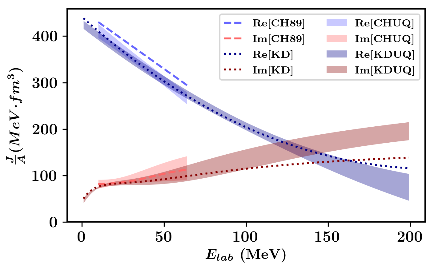
Figure 12: Volume integrals $J/A$ are plotted for CH89, KD, CHUQ, and KDUQ evaluated for neutron scattering on ⁹⁰Zr (all spin-orbit terms are excluded). The CHUQ and KDUQ bands show the 68% uncertainty interval. The ranges of CH89 and CHUQ are restricted to the nominal validity range of CH89 of 10-65 MeV.

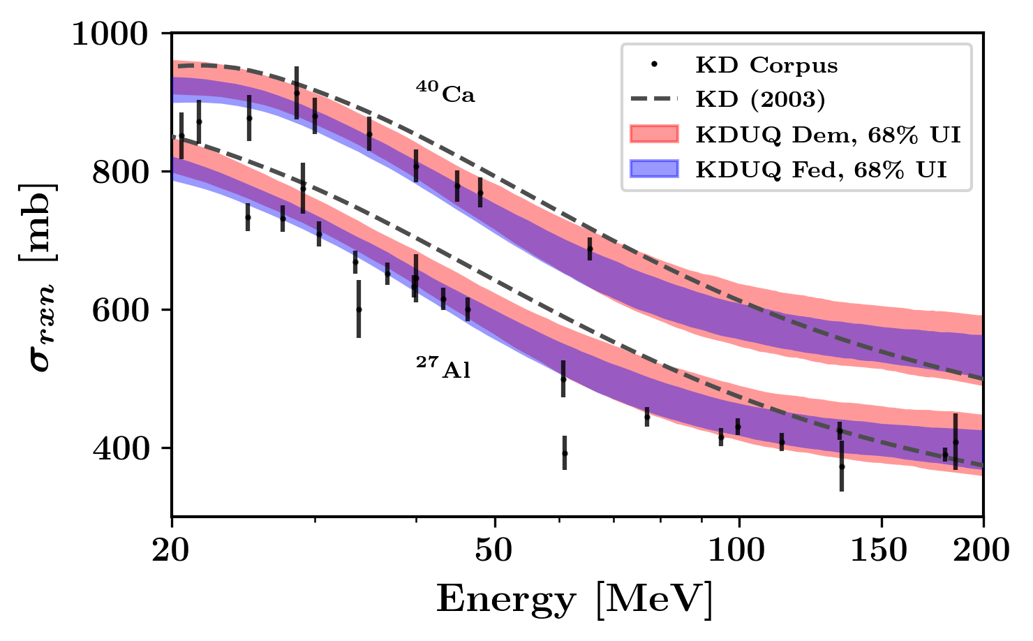
Figure 13: A comparison of KDUQ versions trained using Eq. 11 and Eq. 16 is shown for proton $\sigma_{rxn}$ on ⁴⁰Ca. The 68% and 95% credible intervals of appear as the dark and light bands, respectively. The experimental data of Shane et al. (2010), Pruitt et al. (2020a), and Dietrich et al. (2003) appear as black points with associated errors.

The much-larger uncertainty recovered in CHUQ vs CH89 UQ is indicative of a better match of CHUQ to the breadth of the CHUQ corpus compared to the canonical CH89. However, some important details of the CHUQ corpus and Test corpus are still not captured by CHUQ, due to the relative simplicity of the CH89 potential form. The choice of likelihood in the canonical analysis (Eq. 8) made for good performance of the canonical CH89 parameters with respect to the experimental data, but the lack of normalization in their likelihood function resulted in an underestimation of parametric uncertainty. CHUQ performs moderately well against the Test corpus, considering that the majority of Test corpus data lie outside the nominal validity range of the CH89 potential form, but it is clear that other OMPs should be preferred at energies below 10 .

We now turn to KD and KDUQ. For forty-two out of forty-six parameters, the the canonical value of KD lies within one estimated standard deviation of the KDUQ mean value; of the remaining four, three ($V_{1,\alpha}$, $V_{2,0}^{n}$, and $V_{3,0}^{n}$) are within two estimated standard deviations, and the most discrepant, $W_{1,0}^{n}$, lies just over two estimated standard deviations away. Notably, many sub-term parameters which are coefficients in $E$- and $A$-dependent polynomial expansions are strongly anti-correlated (see KDUQ parameter correlogram in the Supplemental Material Sup ), and their estimated uncertainties are many times larger than their median values. Both these observations indicate overparameterization of $E$- and $A$-dependence in those subterms, so some of these higher-order expansion terms could likely be eliminated without impacting observables. Taken as a whole, the parameter estimates we recover are highly consistent with the canonical ones, which we take as evidence that our replication attempt, though not identical to the canonical treatment, was successful. Further, it confirms that even without the benefit of the computational advances of the last twenty years, the canonical KD analysis was remarkably close to global minimum we recover here.

In the KD/KDUQ functional form, Lane-like asymmetry-dependence appears only in two terms: the first-order energy dependence of the depth of the real volume potential as a function of asymmetry, $V_{1,\alpha}$, and the first-order energy-dependence of the depth of the imaginary surface potential as a function of asymmetry, $D_{1,\alpha}$. For each of these parameters, KDUQ recovers significantly smaller median asymmetry-dependences than those from the canonical treatment. This implies that KD’s real and imaginary surface asymmetry-dependences are weaker than previously assumed, and that the real and imaginary-surface parts of the OMP may be more reliable than previously thought when extrapolated to exotic (near-spherical) targets. At the same time, for $D_{1,\alpha}$, the uncertainties we estimate are almost as large as the median value we recover, indicating that the training data we used (coupled with our analysis assumptions) provides only a weak constraint on the behavior of the imaginary surface term away from the valley of $\beta$-stability. Considering that many downstream applications, such as $r$-process nucleosythesis calculations, fission neutron spectra modeling, and planned transfer and knockout studies at NSCL and FRIB, rely on OMP-informed evaluations of low-energy inelastic cross sections on neutron-rich targets, the fact that $D_{1,\alpha}$ is poorly constrained is a pressing problem. A global, UQ-equipped phenomenological OMP analysis that incorporates isovector-sensitive observables, such as quasi-elastic charge exchange cross sections that have already yielded insight into OMP isovector dependence (e.g., Danielewicz et al. (2017)), is a natural next step.

Besides these terms with explicit asymmetry-dependence, the imaginary volume term, which is separately parameterized for protons and neutrons, contains information about isovector dependence of imaginary strength. For both neutrons and protons, our median-value estimates for first-order imaginary volume strength ($W_{1,0}^{n}$ and $W_{1,0}^{p}$ terms) are moderately larger than the canonical KD value, suggesting enhanced imaginary volume strength overall. Coupled with the smaller overall imaginary surface depth $D_{1,0}$, these result in a reduction in predicted neutron/proton reaction cross sections at low energies (associated with the surface) and an increase at higher energies associated with the volume — in improved agreement with experimental trends for protons shown in Fig. 9. This trend is also visible for neutrons in Fig. 12, where above 100 , the imaginary volume integral grows more rapidly for KDUQ than for KD. If verified, this additional imaginary volume strength would further quench bound-state spectroscopic factors available from dispersive optical models, as discussed in Atkinson and Dickhoff (2019); Pruitt et al. (2020b).

Lastly, to assess the effect of our data covariance matrix ansatz on these interpretations, we compared two different versions of KDUQ: one trained using the “democratic” covariance ansatz of Eq. 11 and one trained using the “federal” covariance ansatz of Eq. 16. Figure 13 shows results from both treatments on predictions of proton $\sigma_{rxn}$ above 50 , where the differences are largest. Overall, these different ansatzes have little effect on the mean parameter values. However, in the case where one training data type has far fewer data than others, the federal ansatz leads to a moderate reduction of unaccounted-for uncertainty required to reproduce data of that type, which leads to more precise predictions for data of that type. This agrees with our expectation that the more realistic the experimental data covariance matrix ansatz is, the less unaccounted-for uncertainty is required to achieve good reproduction of the data.

V Impact

In this section, we apply our UQ-equipped OMPs to two case studies: predicting neutron $\sigma_{tot}$ evolution with respect to asymmetry, and propagation of OMP UQ into Hauser-Feshbach calculations of of (n,$\gamma$) on ⁹⁵Mo and (p,$\gamma$) on ⁸⁷Sr.

V.1 Case study 1: evolution of neutron total cross sections in isotopic pairs

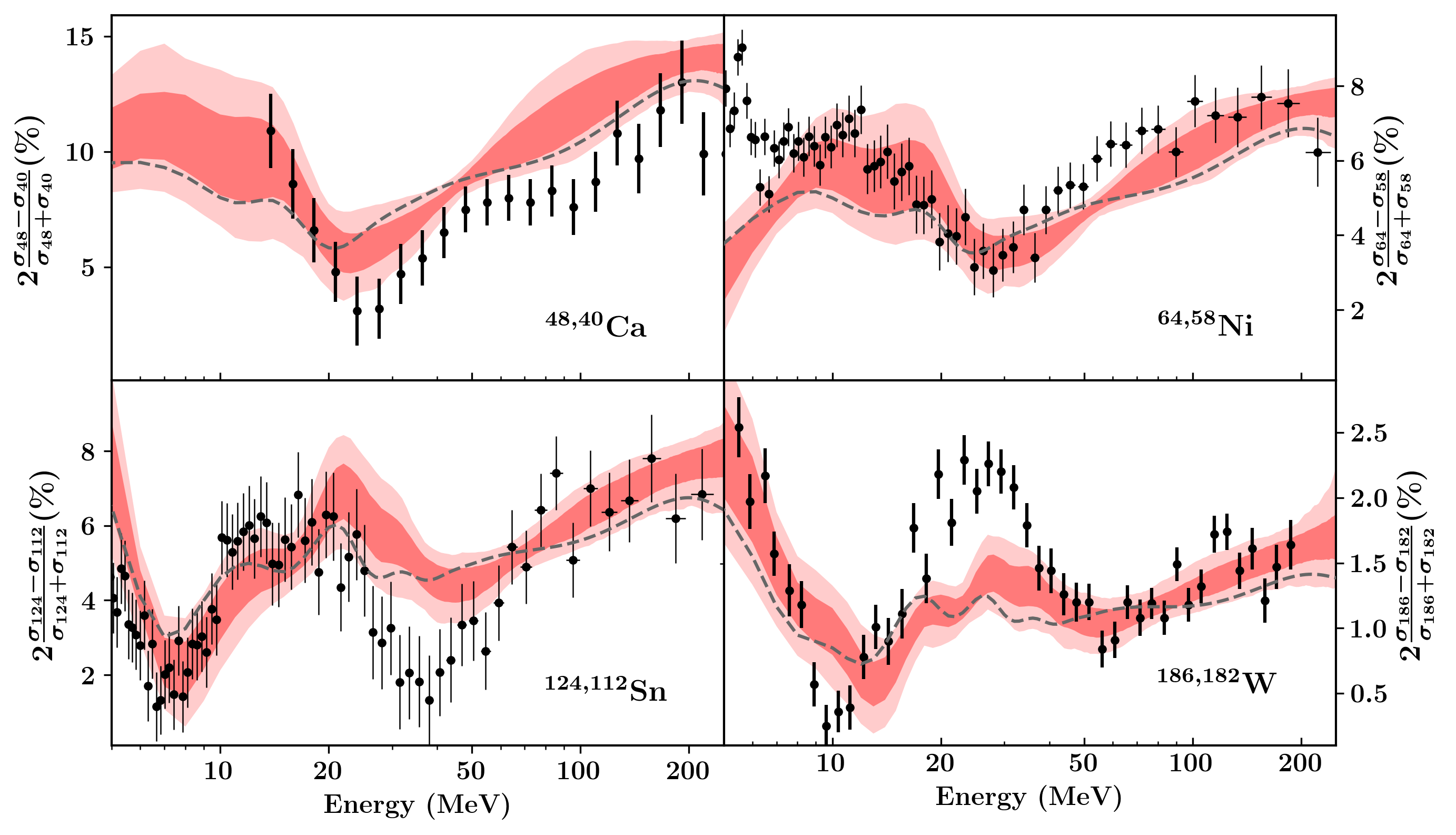
Figure 14: Relative differences of neutron total cross sections from 5 to 250  for several isotopic pairs are plotted. Calculations using the standard Koning-Delaroche global potential are shown via the gray dashed line. The 68% and 95% credible intervals of KDUQ appear as the dark and light red bands, respectively. The experimental data of Shane et al. (2010), Pruitt et al. (2020a), and Dietrich et al. (2003) appear as black points with associated errors.

Cross sections for neutron-induced reactions on $\beta$-unstable targets are a key input for several nuclear data applications, e.g., $r$-process nucleosynthesis network calculations Surman et al. (2014). Because of the experimental difficulty in performing cross section measurements in this regime, cross sections estimations rely on either (semi-)microscopic OMPs Jeukenne et al. (1977); Bauge et al. (2001) or phenomenological potentials fitted solely to stable-target data, such as the KD global OMP, that are then extrapolated according to their assumed asymmetry-dependence. For incident neutrons at lower energies ($<10$ ), the asymmetry-dependence of the imaginary surface term strongly affects capture cross sections Goriely and Delaroche (2007), but the magnitude of this asymmetry-dependence remains poorly known. More broadly, such isovector components of optical potentials are connected to other poorly constrained but important nuclear quantities, such as neutron skins in finite nuclei Dietrich et al. (2003); Atkinson and Dickhoff (2019); Pruitt et al. (2020b) and the density-dependence of the symmetry energy, $L$, in nuclear matter, which influences both the theoretical limit to neutron star radii and the dynamics of neutron star mergers, among other properties Thiel et al. (2019). As such, improving our knowledge of the appropriate asymmetry-dependence of OMPs remains an important task.

To constrain asymmetry-dependent terms of phenomenological OMPs, past analyses have focused mainly on two types of experimental data: quasielastic charge exchange cross sections to the isobaric analog state (as analyzed in Danielewicz et al. (2017) using a KD-like potential), and ratios of neutron cross sections measured on different isotopes along an isotopic or isotonic chain (as studied by Camarda et al. (1984); Shamu et al. (1980); Dietrich et al. (2003); Shane et al. (2010); Pruitt et al. (2020a)). Quasielastic charge exchange is an ideal probe in that measured cross sections are sensitive specifically to isovector strength, but analysis of these data may require more sophisticated theoretical machinery (as compared to straightforward elastic and total cross section calculations) to correct for contamination from $\Delta J^{\pi}\neq 0^{+}$ channels, as demonstrated in Jon et al. (1997). The second type, ratios of neutron cross sections, has the advantage that by taking a cross section ratio, many systematic uncertainties (such as detector efficiency) are divided out. Further, if more than two isotopic targets are available, multiple ratios can be constructed and additional quantities, such as degree of deformation, can be extracted Camarda et al. (1984); Shamu et al. (1980). In addition, because neutron total cross sections can be simultaneously collected from a few to a few hundred Finlay et al. (1993); Abfalterer et al. (2001) at precisions of $\approx 1\%$, ratios of neutron total cross sections can provide information about OMP isovector features across broad regime of energies relevant for OMP construction and application. The main drawback of this type of measurement is the often-prohibitive expense of obtaining large, isotopically pure targets with precisely known areal densities. Even when isotopically pure targets are available along an isobar or isotopic chain, because they must be stable or at least long-lived to be suitable for target fabrication, they can span only a small range of asymmetries, which diminishes the isovector signal in the cross section ratio.

The importance of constraining isovector terms warrants a future, global OMP analysis including both of these data types as well as neutron strength functions (as used by Bauge et al. (2001)) to characterize isovector dependence. As a precursor to such an analysis, in Fig. 14 we consider canonical KD OMP and KDUQ predictions against neutron total cross section isotopic ratios on ^40,48Ca Shane et al. (2010), ^58,64Ni, ^112,124Sn, Pruitt et al. (2020a), ^182,186W Dietrich et al. (2003). In all instances, the median predicted value from KDUQ closely follows the canonical KD predictions. Due to the small reported uncertainties of the experimental data shown in Fig. 14, the canonical KD predictions are discrepant with the experimental data at the several-$\sigma$ level in many places, e.g., the ⁶⁴Ni-⁵⁸Ni relative difference below 20  in panel (b). As such, if one considers just the canonical KD curve, one might conclude that the KD potential form is missing some important asymmetry-dependent physics that are present in the data. However, when OMP parametric uncertainties are considered (as shown in the KDUQ curve), it is clear that most of the discrepancies between the canonical KD predictions and experimental data are not statistically meaningful. That is, once parameter uncertainties are included, the KD potential form is quite effective at predicting these cross section ratios to which it was never trained. Moreover, any discrepancies that remain after parametric uncertainty is considered (for example, the overprediction of the Sn isotopic ratios, shown in panel (c), between 30 and 50 ), become even more interesting: they do indicate residual physics that has been captured by the measurement, but not by the assumptions of our OMP. In the specific case of Sn and W isotopic ratios, the likely cause for the significant discrepancy between predictions and measurements is that the KD form, by definition, neglects the differing density profiles for neutron and protons in the Sn and W isotopes. Indeed, Dietrich et al. Dietrich et al. (2003) who collected the W data found that accurately reproducing the W isotopic ratio data between 20 and 40  required a Jeukenne-Lejeune-Mahaux-inspired coupled-channel OMP analysis that featured an increasing neutron skin from ¹⁸²W to ¹⁸⁶W. If more isotopically resolved neutron total cross section ratios were available, a similar analysis across many isotopic chains could provide neutron skin thicknesses and additional information on $L$, though the potential would need to be deformation-aware and not spherical, as assumed here. The apparent (but, in light of the parametric uncertainty, insignificant) discrepancy between the canonical KD calculation and the Ni isotopic ratio data is an example of how well-calibrated UQ helps avoid mistaking noise in the experimental data for signal. At the very least, the KDUQ predictions make clear that in order for neutron total cross section ratios to constrain asymmetry-dependent OMP terms for a KD-like potential, the relative difference measurement must achieve 1% precision or better.

V.2 Case study 2: ⁹⁵Mo(n,$\gamma$)⁹⁶Mo and ⁸⁷Sr(p,$\gamma$)⁸⁸Y cross sections

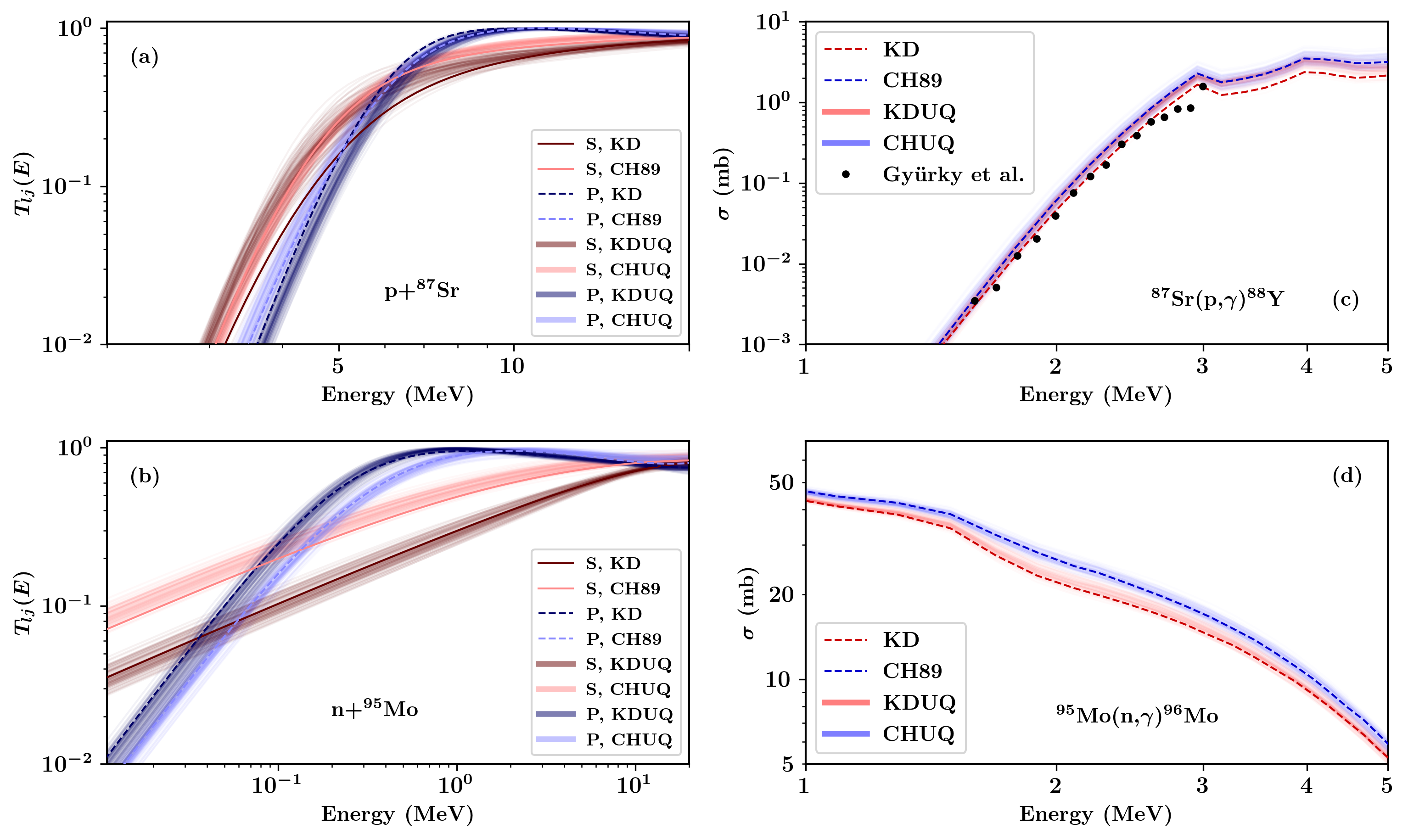
Figure 15: Transmission coefficients and cross sections for ⁸⁷Sr(p,$\gamma$)⁸⁸Y and ⁹⁵Mo(n,$\gamma$)⁹⁶Mo are plotted. All calculations were performed using the statistical reaction code YAHFC Ormand with default structure inputs. Calculations using the canonical Koning-Delaroche OMP are shown via blue lines; calculations using CH89 are shown as red lines. Calculations using 100 samples each from the KDUQ and CHUQ posterior distributions are shown as diffuse blue and red bands, respectively. In panels (a) and (b), both $S$-wave (L=0, J=$\frac{1}{2}$) and $P$-wave (L=1, J=$\frac{3}{2}$) transmission coefficient curves are shown. Panel (c) includes experimental data from Gyürky et al. Gyürky et al. (2001) (scaled upward by a factor of 2.5 to agree with the ⁸⁸Sr(p,$\gamma$)⁸⁹Y data of Galanopoulos et al. (2003), as indicated by Vagena et al. Vagena et al. (2021)).

One of the most common applications for OMPs is as an input for radiative capture calculations. While direct and pre-equilibrium capture mechanisms play an important role for light and near-dripline nuclei Xu et al. (2014), the Hauser-Feshbach model, which assumes equilibration of the excited composite nucleus before de-excitation, is appropriate for most nucleon capture reactions. In this picture, both the probability of creating a compound nucleus in the entrance channel and the evaporation of nucleons from an excited nucleus depend on energy- and angular-momentum-dependent transmission coefficients $T_{lj}(E)$ that are determined by an OMP. To illustrate the relative impact of OMP uncertainty on nucleon capture within the Hauser-Feshbach model, we propagated CHUQ and KDUQ uncertainties through two representative reactions: ⁹⁵Mo(n,$\gamma$)⁹⁶Mo and ⁸⁷Sr(p,$\gamma$)⁸⁸Y at incident nucleon energies up to 5 . Calculations were carried out using the LLNL Hauser-Feshbach code YAHFC Ormand , modified to accept KD-like and CH89-like potentials with arbitrary parameters, and using YAHFC default configuration information, discrete level data, nuclear level densities (LDs), and $\gamma$-ray strength functions ($\gamma$SFs). For each reaction, we ran YAHFC once using the canonical KD and once using the canonical CH89 potential and then performed one hundred YAHFC runs each for CHUQ and KDUQ, with each run using a unique sample of the OMP parameter posterior. Results of these calculations are shown in Fig. 15. Panels (a) and (b) show transmission coefficients $T_{lj}(E)$ generated by YAHFC’s invocation of frescox Thompson for protons incident on ⁸⁷Sr and for neutrons incident on ⁹⁵Mo. Panels (c) and (d) display the corresponding capture cross sections, where the uncertainty shown is due to the transmission coefficients of panels (a) and (b). As YAHFC uses a Monte Carlo approach for de-exciting compound nuclei, we drew $10^{6}$ samples at each scattering energy to ensure that YAHFC’s statistical uncertainty due to Monte Carlo sampling was less than 1% for the calculated capture cross sections.

For p+⁸⁷Sr, the CH89, CHUQ, and KDUQ transmission coefficients show overall consistency across all depicted energies, whereas the KD transmission coefficients are slightly lower than the other OMPs between 3 and 10 . The principle difference for KD was reduced $s$-wave strength and a more rapid rise in $p$-wave strength. Below 3   the Coulomb barrier manifests as a steep reduction across the board. Above 10  (the minimum energy included in the CHUQ corpus), the $T_{lj}(E)$ generated from all four OMPs are consistent within approximately 10%, an indication that the OMP uncertainty is likely a minor source of uncertainty in cross section predictions above this energy.

This reaction was one of those considered by Vagena et al. in their recent study Vagena et al. (2021) of systematic effects of the proton OMP on $p$-process nucleosynthesis. In their approach, using talys they sought to improve the Bruyére-le-Châtel version of the Jeukenne-Lejeune-Mahaux semi-microscopic proton OMP Bauge et al. (2001) by tuning its parameters to better reproduce experimental cross sections for specific reactions. In the case of ⁸⁷Sr(p,$\gamma$)⁸⁸Y, experimental data were available from 1.6 to 3  as collected by Gyürky et al., shown here in panel (c) of Fig. 15. Following Vagena et al., we have scaled the data up by a factor of 2.5 from the original publication to comport with ⁸⁸Sr(p,$\gamma$)⁸⁹Y data subsequently published by Galanopoulos et al. (2003). In their analysis, they argued that below roughly 3 , this reaction can be considered independent of the ⁸⁸Sr LD and $\gamma$SF, so any remaining discrepancy between predictions and measured data serves as a basis for adjusting OMP parameters. In our case, while we did not perform calculations using any microscopic OMPs, all four global phenomenological OMPs we did consider – CH89, CHUQ, KD, and KDUQ – generate predictions within a few tens of percent of the experimental cross sections. This suggests that unless both the LD and $\gamma$SF are known within a few tens of percent precision for a given reaction, constraining OMP parameters by working backwards from measured capture cross sections may not be feasible. A consistent joint treatment combining all of these sources of uncertainty is a next step in which the yet-unknown correlations between OMPs, LDs, and $\gamma$SFs will be critically important. We hope to engage in a systematic study following the logic of Vagena et al. (2021) that compares microscopic OMPs with UQ-equipped phenomenological ones for astrophysically relevant reactions. At the very least, we argue that the intuition provided here on standard phenomenological OMPs can guide analysts interested in manually tuning microscopic OMP parameters to reproduce experimental scattering observables. Given our finding that the CH89 and KD uncertainty effect on capture cross sections between 1-5  that we examined is on the order of tens of percent, a practitioner who encounters a larger discrepancy between their prediction and experimental data should consider other sources of uncertainty beyond the OMP parameters, such as deformation or level density uncertainty.

Finally, we consider n+⁹⁵Mo in panels (b) and (d). Throughout the depicted energy range, CHUQ calculations are highly consistent with CH89 and KDUQ calculations with KD, but both KD-type OMPs have a much slower rise in $s$-wave strength with respect to energy than do the CH89-type OMPs. At energies above 100   the slower $s$-wave rise is offset by a correspondingly faster rise in $p$-wave strength such that resulting neutron cross section predictions, which include contributions over all incident partial waves, differ by only 20-30%, highly consistent with the degree of uncertainty seen for p+⁸⁷Sr. Importantly, for any reactions at energies below 100  involving primarily the $s$-wave transmission coefficients, CH89 and CHUQ are expected to yield a cross section two to three times higher than KD and KDUQ. In such case, the OMP uncertainty should indeed dominate the cross section, as uncertainty in the LDs and $\gamma$SFs have minimum impact at lower energies (again shown in Fig. 1 and 2 of Vagena et al. Vagena et al. (2021)). Such OMP-driven uncertainty could impact both weak and strong $r$-process network calculations. Comparison of the canonical KD OMP’s $s$- and $p$-wave strength functions against experimental data, as shown in Fig. 47 of Koning and Delaroche’s original analysis, suggest that at energies below 100 , KD-type OMPs may have a more realistic energy dependence than the CH89-type OMPs. A detailed study of OMPs uncertainty at nucleosynthetic “bottlenecks” seems a worthy follow-up.

VI Conclusions

Phenomenological OMPs continue to play an important role in nuclear reaction calculations but lack well-calibrated UQ. Without reliable uncertainty estimates, it is difficult to assess the relative importance of OMPs on the overall uncertainty budget of applications dependent on reaction data. To address this issue, we identified two main obstacles – systematic underestimation of experimental (co)variance and a lack of outlier rejection – and developed a generic pipeline for performing UQ on phenomenological OMPs. We then applied it to the widely-used CH89 and KD global OMPs, yielding two new potential ensembles, CHUQ and KDUQ, with full covariance information between potential parameters. CHUQ and KDUQ perform favorably against their training corpora, with KDUQ showing superior performance on the Test corpus, especially for proton $\sigma_{rxn}$ and neutron $\sigma_{tot}$. Accordingly, we recommend using KDUQ over CHUQ for non-elastic calculations and for calculations below 10  (the stated threshold of validity for CH89). In the case of proton $\sigma_{rxn}$ data, KDUQ shows improved performance compared to the canonical KD global OMP. Further, by training two versions of KDUQ with different assumed forms of data covariance, we demonstrated how small changes in underlying covariance assumptions can impact the uncertainty of predictions in data-sparse regions, as shown for high-energy proton $\sigma_{rxn}$ in Fig. 13. These results caution against naïve use of a weighted-least-squares likelihood function when experimental data used for training are known to have underestimated uncertainties and non-trivial covariance structure. In the case we presented, an MCMC-based inference strategy made sense so that we could include our unaccounted-for uncertainty estimates as priors, but the need for a defensible likelihood function is just as important in any approach, Bayesian or not, involving training a model to data.

As a demonstration of their utility, we forward-propagated CHUQ and KDUQ’s parameter covariances in two case studies. In the first, we showed that KDUQ accurately predicts neutron $\sigma_{tot}$ evolution with respect to asymmetry, auguring well for neutron-scattering predictions beyond the valley of $\beta$-stability, at least along closed shells in $Z$. Because our uncertainty-quantified model was designed to incorporate the observed variance of its training data, a discrepancy between our model and experimental data is not easily explained away as arbitrariness in the model parameters. For example, in our examination of isotopic relative differences of neutron $\sigma_{tot}$, we saw KDUQ underpredicted the oscillations present in the experimental relative differences for Sn and W isotopes between $20$ and $50$  (panels (c) and (d) of Fig. 14). These oscillations can be reproduced by an OMP analysis only if the different proton and neutron density distributions of the target are taken into account, as shown in Dietrich et al. (2003). Although this physics is absent from the KD or CH89 pictures, it implies that, provided one uses an uncertainty-quantified OMP and fits to relative $\sigma_{tot}$ differences rather than absolute cross sections, neutron $\sigma_{tot}$ data are useful for extracting neutron skin thickness information. As new reactions are pursued at modern radioactive beam facilities, this kind of comparison between uncertainty-equipped data and uncertainty-equipped models is important for calibrating our “degree of surprise” to avoid chasing down spurious signals. Systematic comparison against isovector data, including (p,n) cross sections and $\sigma_{tot}$ relative differences along isotopic and isotonic chains, is a promising meeting-ground for phenomenological and microscopic OMPs.

Finally, we explored the impact of KDUQ and CHUQ on representative radiative capture calculations for ⁸⁷Sr and ⁹⁵Mo. The capture cross sections between 1-5  computed using KDUQ are somewhat lower ($\approx 20-30\%$) than those using CHUQ, though with substantial uncertainty overlap. Given the systematic assessment of proton capture rate uncertainty of Vagena et al. (2021), we argue that in the few- range, the fraction of overall cross section uncertainty due to the OMP is comparable to that in the $\gamma$-ray strength function and level density, and at energies below 1  the OMP uncertainty may dominate. Moreover, while the partition of strength between $s$- and $p$-wave below 10  are different, particularly for neutrons, the contributions from each to the overall cross sections were countervailing for ⁹⁵Mo. If angular momentum transfer is restricted to a single partial wave, the differences between (and uncertainty in) OMPs can be much larger, as shown for n+⁹⁵Mo below 100 , and the effect on cross sections correspondingly larger. This is another region where comparison between (semi)-microscopic and phenomenological OMPs is likely to be fruitful, both for improving existing OMPs and for providing more stringent reaction rates to astrophysical nucleosynthesis calculations. To support such efforts, we enclose copies of CHUQ and KDUQ in the Supplemental Material Sup .

Appendix A Definition of optical potentials and scattering formulae

Reproduced here are the definition of the Chapel Hill ’89 Varner et al. (1991) and Koning-Delaroche Koning and Delaroche (2003) optical potentials, starting from the overall potential form and ending with the definitions for form subterms. Free parameters (those subject to Bayesian inference via MCMC) are denoted in this section using a bold typeface. For brevity we set $\hbar=c=1$.

A.1 CH89 definition

The CH89 global optical potential for single-nucleon scattering consists of five terms:

$$\begin{split}\mathcal{U}(r,E)=&\mathcal{V}_{r}(r,E)-i\mathcal{W}_{v}(r,E)-i\mathcal{W}_{s}(r,E)\\ -&\mathcal{V}_{so}(r,E)(\ell\cdot\sigma)+\mathcal{V}_{C}(r),\end{split}$$ (22)

where

• $\mathcal{V}_{r}$ is the real central potential,

• $\mathcal{W}_{v}$ is the imaginary central (or “volume”) potential,

• $\mathcal{W}_{s}$ is the imaginary surface potential,

• $\mathcal{V}_{so}$ is the real spin-orbit potential, and

• $\mathcal{V}_{C}$ is the Coulomb potential (for protons only).

As with the Koning-Delaroche potential defined below, each component (except Coulomb) consists of an energy-dependent depth coupled with a radius-dependent spatial form:

$$\begin{split}\mathcal{V}_{r}(r,E)&=V_{r}(E)\times f(r,R_{0},\mathbf{a_{0}}),\\ \mathcal{W}_{v}(r,E)&=W_{v}(E)\times f(r,R_{w},\mathbf{a_{w}}),\\ \mathcal{W}_{s}(r,E)&=W_{s}(E)\times-4\mathbf{a_{w}}\frac{d}{dr}f(r,R_{w},\mathbf{a_{w}}),\\ \mathcal{V}_{so}(r,E)&=2V_{so}\times\frac{-1}{r}\frac{d}{dr}f(r,R_{so},\mathbf{a_{so}}),\\ \mathcal{V}_{C}(r)&=\begin{cases}\frac{Zze^{2}}{2R_{C}}\left(3-\frac{r^{2}}{R_{C}^{2}}\right),&\text{if }r<R_{C}\\ \frac{Zze^{2}}{r},&\text{if }r\geq R_{C}\end{cases}.\end{split}$$ (23)

The spatial form $f(r,R,a)$ is the standard Woods-Saxon potential

$$\begin{split}f(r,R,a)&=\frac{1}{1+e^{(r-R)/a}},\\ \frac{d}{dr}f(r,R,a)&=\frac{1}{a}\left[\frac{-e^{(r-R)/a}}{(1+e^{(r-R)/a})^{2}}\right].\end{split}$$ (24)

Here $R$ and $a$ are radius and diffuseness parameters, respectively. The usual $R=r_{0}A^{1/3}$ dependence is assumed (see Eq. 27 below for equations defining $r_{0}$ for each component), with $A$ the nucleon number of the target. We note that for a natural-abundance target, the value that should be taken for $A$ is not explicitly discussed in the original formulation of CH89 or KD. A simple choice would be to use the $A$ of the most abundant isotope, which works well for many elements but is unsatisfying in cases where the lightest or heaviest isotope is most abundant. For example, in ${}^{\text{nat}}$Ni the most abundant isotope is ⁵⁸Ni, but the abundance-weighted nucleon number is 58.76 (a difference of 1.3% from 58). In this work, for natural targets we took for $A$ the target’s atomic weight, which for the targets we used agrees with the abundance-weighted nucleon number to within $\approx 0.1\%$.

The CH89 energy-dependent depths are given by:

$$\begin{split}V_{r}(E)&=\mathbf{V_{0}}+\mathbf{V_{e}}\Delta E\pm\alpha\mathbf{V_{t}}\\ W_{v}(E)&=\mathbf{W_{v0}}\left[1+e^{\frac{\mathbf{W_{ve0}}-\Delta E}{\mathbf{W_{vew}}}}\right]^{-1}\\ W_{s}(E)&=(\mathbf{W_{s0}}+\alpha\mathbf{W_{st}})\left[1+e^{\frac{\Delta E-\mathbf{W_{se0}}}{\mathbf{W_{sew}}}}\right]^{-1}\\ V_{so}(E)&=\mathbf{V_{so0}}\end{split}$$ (25)

The nuclear asymmetry $\alpha$ is defined $(N-Z)/A$. As with the definition of $A$, for natural targets a definition for $\alpha$ is not given in the original potential formulation. For these targets, we took $\alpha=(A-2Z)/Z$, consistent with our definition of $A$. The energy argument $\Delta E$ is the difference between the scattering energy and the volume-averaged Coulomb energy:

$$\begin{split}\Delta E&=E_{lab}-E_{c}\\ E_{c}&=\begin{cases}\frac{6Ze^{2}}{5R_{c}},&\text{for protons}\\ 0,&\text{for neutrons}\end{cases}.\end{split}$$ (26)

Lastly, the radial form parameters $R_{i}$ are defined as follows:

$$\begin{split}R_{0}=\mathbf{r_{0}}A^{1/3}+\mathbf{r_{0}^{0}},\\ R_{w}=\mathbf{r_{w}}A^{1/3}+\mathbf{r_{w}^{0}},\\ R_{so}=\mathbf{r_{so}}A^{1/3}+\mathbf{r_{so}^{0}},\\ R_{C}=\mathbf{r_{c}}A^{1/3}+\mathbf{r_{c}^{0}}.\end{split}$$ (27)

In total there are 22 free potential parameters: 11 associated with the potential depths and 16 associated with the radius-dependent spatial forms. We comment that in the original CH89 treatment, only 20 parameters were free, as the authors fixed the Coulomb parameters $r_{c}$ and $r_{c}^{(0)}$ based on a separate assessment.

A.2 Koning-Delaroche definition

Similar to CH89, the Koning-Delaroche optical potential for single-nucleon scattering is defined as a function of radius $r$ and energy $E$:

$$\begin{split}\mathcal{U}(r,E)&=-\mathcal{V}_{V}(r,E)-i\mathcal{W}_{V}(r,E)-i\mathcal{W}_{D}(r,E)\\ &+\mathcal{V}_{SO}(r,E)(\ell\cdot\sigma)+i\mathcal{W}_{SO}(r,E)(\ell\cdot\sigma)+\mathcal{V}_{C}(r),\end{split}$$ (28)

where

• $\mathcal{V}_{V}$ is the real central potential,

• $\mathcal{W}_{V}$ is the imaginary central potential,

• $\mathcal{W}_{D}$ is the imaginary surface potential,

• $\mathcal{V}_{SO}$ is the real spin-orbit potential,

• $\mathcal{W}_{SO}$ is the imaginary spin-orbit potential, and

• $\mathcal{V}_{C}$ is the Coulomb potential (for protons only).

In the spin-orbit components, $\ell$ is the orbital angular momentum quantum number for each partial wave associated with the incident projectile and $\sigma$ is the spin of the incident projectile. Except Coulomb, each component consists of an energy-dependent depth coupled with a radius-dependent spatial form:

$$\begin{split}\mathcal{V}_{V}(r,E)&=V_{V}(E)\times f(r,R_{V},a_{V}),\\ \mathcal{W}_{V}(r,E)&=W_{V}(E)\times f(r,R_{V},a_{V}),\\ \mathcal{W}_{D}(r,E)&=W_{D}(E)\times-4a_{D}\frac{d}{dr}f(r,R_{D},a_{D}),\\ \mathcal{V}_{SO}(r,E)&=V_{SO}(E)\left(\frac{\hbar}{m_{\pi}c}\right)^{2}\times\frac{1}{r}\frac{d}{dr}f(r,R_{SO},a_{SO}),\\ \mathcal{W}_{SO}(r,E)&=W_{SO}(E)\left(\frac{\hbar}{m_{\pi}c}\right)^{2}\times\frac{1}{r}\frac{d}{dr}f(r,R_{SO},a_{SO}),\\ \mathcal{V}_{C}(r)&=\begin{cases}\frac{Zze^{2}}{2R_{C}}\left(3-\frac{r^{2}}{R_{C}^{2}}\right),&\text{if }r<R_{C}\\ \frac{Zze^{2}}{r},&\text{if }r\geq R_{C}\end{cases}.\end{split}$$ (29)

The spatial form $f(r,R,a)$ is the same Woods-Saxon defined earlier in the CH89 case (Eq. 24), with $R=r_{0}A^{1/3}$. In the spin-orbit subcomponent definitions, $m_{\pi}$ is the charged pion mass. In the Coulomb component definition, $z$ is the projectile charge, $Z$ is the target charge, and $e^{2}$ is the elementary charge squared ($\approx$ 1.44 $\cdot$ f ).

Depending on whether the user is modeling neutron or proton scattering, the energy-dependent depths appearing in Eq. 29 are given by:

$$\begin{split}V_{V}(E)=v_{1}^{n,p}&[1-v_{2}^{n,p}\Delta E^{n,p}\\ &+v_{3}^{n,p}(\Delta E^{n,p})^{2}-v_{4}^{n,p}(\Delta E^{n,p})^{3}]\\ +\overline{V}_{C}&\times v_{1}^{p}[v_{2}^{p}-2v_{3}^{p}\Delta E^{p}+3v_{4}^{p}(\Delta E)^{2}]\\ W_{V}(E)&=w_{1}^{n,p}\frac{(\Delta E)^{2}}{(\Delta E)^{2}+(w_{2}^{n,p})^{2}},\\ W_{D}(E)&=d_{1}^{n,p}\frac{(\Delta E)^{2}}{(\Delta E)^{2}+(d_{3}^{n,p})^{2}}e^{-d_{2}^{n,p}\Delta E},\\ V_{SO}(E)&=v_{so1}^{n,p}e^{-v_{so2}^{n,p}\Delta E},\\ W_{SO}(E)&=w_{so1}^{n,p}\frac{(\Delta E)^{2}}{(\Delta E)^{2}+(w_{so2}^{n,p})^{2}},\end{split}$$ (30)

where the superscripts $n,p$ denote different parameters used for neutrons and protons, respectively. The energy variable $\Delta E^{n,p}$ is the difference between the incident scattering energy in  in the lab frame and the Fermi energy for neutrons or protons:

$$\begin{split}\Delta E^{n,p}&=E-E_{f}^{n,p}\\ E_{f}^{n}&=-11.2814+0.02646A\\ E_{f}^{p}&=-8.4075+1.01378A.\end{split}$$ (31)

The potential depth parameters from Eq. 30 are defined as:

$$\begin{split}v_{1}^{n,p}&=\mathbf{v_{1,0}}-\mathbf{v_{1,A}}A\pm\mathbf{v_{1,\bm{\alpha}}}\alpha\\ v_{2}^{n,p}&=\mathbf{v_{2,0}^{n,p}}\pm\mathbf{v_{2,A}^{n,p}}\\ v_{3}^{n,p}&=\mathbf{v_{3,0}^{n,p}}\pm\mathbf{v_{3,A}^{n,p}}\\ v_{4}^{n,p}&=\mathbf{v_{4,0}}\\ w_{1}^{n,p}&=\mathbf{w_{1,0}^{n,p}}+\mathbf{w_{1,A}^{n,p}}A\\ w_{2}^{n,p}&=\mathbf{w_{2,0}}+\mathbf{w_{2,A}}A\\ d_{1}^{n,p}&=\mathbf{d_{1,0}}\pm\mathbf{d_{1,\bm{\alpha}}}\alpha\\ d_{2}^{n,p}&=\mathbf{d_{2,0}}+\frac{\mathbf{d_{2,A}}}{1+e^{(A-\mathbf{d_{2,A3}})/\mathbf{d_{2,A2}}}}\\ d_{3}^{n,p}&=\mathbf{d_{3,0}}\\ v_{so1}^{n,p}&=\mathbf{v_{so1,0}}+\mathbf{v_{so1,A}}A\\ v_{so2}^{n,p}&=\mathbf{v_{so2,0}}\\ w_{so1}^{n,p}&=\mathbf{w_{so1,0}}\\ w_{so2}^{n,p}&=\mathbf{w_{so2,0}}\\ \overline{V}_{C}&=\frac{V_{C}Z}{r_{C}A^{1/3}}=\frac{6Ze^{2}}{5r_{C}A^{1/3}}.\end{split}$$ (32)

In these expressions, $\pm$ should be taked as $-$ for neutrons and $+$ for protons. Our definitions for $A$ and for the nuclear asymmetry $\alpha$ for natural targets are the same as used above for CH89.

Finally, the radial form parameters entering Eqs. 24 and 29 are defined

$$\begin{split}r_{V}&=\mathbf{r_{V,0}}-\mathbf{r_{V,A}}A^{-1/3}\\ a_{V}&=\mathbf{a_{V,0}}-\mathbf{a_{V,A}}A\\ r_{D}&=\mathbf{r_{D,0}}-\mathbf{r_{D,A}}A^{-1/3}\\ a_{D}&=\mathbf{a_{D,0}^{n,p}}\pm\mathbf{a_{D,A}^{n,p}}A\\ r_{SO}&=\mathbf{r_{SO,0}}-\mathbf{r_{SO,A}}A^{-1/3}\\ a_{SO}&=\mathbf{a_{SO,0}}\\ r_{C}&=\mathbf{r_{C,0}}+\mathbf{r_{C,A}}A^{-2/3}+\mathbf{r_{C,A2}}A^{-5/3}.\end{split}$$ (33)

As in Eq. 32, $\pm$ should be taken as $-$ for neutrons and $+$ for protons. In total there are 47 free potential parameters: 31 associated with the energy-dependent depths and 16 associated with the radius-dependent spatial forms.

A.3 Scattering formulae

In this section we list the expressions we used to calculate proton and neutron scattering observables. Our procedure follows the calculable $R$-matrix method outlined in Descouvement and Baye (DB) Descouvement and Baye (2010), but modified (as discussed below) to be suitable for relativistic-equivalent calculations. The scattering observables we considered can all be calculated from the scattering matrix for incident partial waves. The $S$ matrix for the incident projectile partial wave with angular momentum $l$ is (DB Eq. 3.24):

$$S_{l}=e^{2i\delta_{l}}=e^{2i\phi_{l}}\frac{1-(L_{l}^{*}-B)R_{l}(E,B)}{1-(L_{l}-B)R_{l}(E,B)}.$$ (34)

The $S$-matrix terms are equivalent to the partial wave phase shifts $\delta_{l}$. Here $L_{l}$ is the logarithmic derivative of the outgoing partial wave, evaluated at channel radius $a$. It can be expressed in terms of Coulomb functions (DB Eqs. 3.28-3.30):

$$\begin{split}L_{l}&=\frac{ka}{F_{l}(ka)^{2}+G_{l}(ka)^{2}}\\ &\times\left[F_{l}(ka)F_{l}^{\prime}(ka)+G_{l}(ka)G_{l}^{\prime}(ka)+i\right].\end{split}$$ (35)

The hard-sphere phase shift, $\phi_{l}$, is (DB Eq. 3.26)

$$\phi_{l}=-\tan^{-1}(F_{l}(ka)/G_{l}(ka)).$$ (36)

In these expressions, $F_{l}$ and $G_{l}$ are the regular and irregular Coulomb functions, with $F^{\prime}_{l}$ and $G^{\prime}_{l}$ their derivatives. (In the Coulomb function notation, we have omitted the implied Sommerfeld parameter $\eta$.) $R_{l}(E,B)$ are the $R$-matrix elements, discussed below, and $B$ is a dimensionless boundary parameter associated with the Bloch operator. As shown in Eq. 3.27 and appendix B of DB, the scattering matrix is unaffected by the choice of boundary parameter $B$, so $B$ can be set to 0 to simplify the $S$- and $R$-matrix calculation algebra.

To calculate the $R$ matrix, we used the finite-basis approximation (Eq. 3.15 in DB):

$$R_{l}(E,B)=\frac{1}{2\mu a}\sum^{N}_{i,j=1}\phi_{i}(a)(\bm{C}^{-1})_{ij}\phi_{j}(a).$$ (37)

Here $E$ is the center-of-mass energy, $\mu$ is the reduced mass, $a$ is the channel radius, $N$ is the number of basis states $\phi$, and $\bm{C}$ is the symmetric matrix containing solutions to the inhomogenous Bloch-Schrödinger equation (Eq. 3.7 in DB),

$$\bm{C}_{i,j}(E,B)=\bra{\phi_{i}}T_{l}+\mathcal{L}(B)+V-E\ket{\phi_{j}}$$ (38)

To solve this equation, we employed the Lagrange-mesh method of Baye Baye (2015) on an $N=30$ Legendre-polynomial mesh. The kinetic energy $T_{l}$ and Bloch $\mathcal{L}(B)$ operators on this Lagrange-Legendre mesh (which we do not reproduce here) are given by Eqs. 3.127 and 3.129 of Baye (2015). In our case, $V$ is the optical potential, with $E$ the center-of-mass energy. Note, however, that the energy argument of the optical potential, e.g., $E$ in $U(r,E)$ of Eq. 28, is the projectile energy in the lab frame, per the definition of CH89 and KD.

The above formulation is appropriate for the non-relativistic limit, but above a few tens of , an approximate relativistic-equivalent version should be used, requiring modification of several elements in the calculation. First, the center-of-mass energies, angles, and the relative velocity appearing in the Sommerfeld parameter should be calculated according to relativistic kinematics. Second, in the relativistic picture the reduced mass and center-of-mass wavenumber are no longer suitable to describe the relative motion between projectile and target, so approximations are required. We used the relativistic approximations of Eqs. 17 and 20 in Ingemarsson’s topical study Ingemarsson (1974) that base the wavenumber on the relativistic momentum in the center-of-momentum frame and treat the center-of-momentum motion of the target as non-relativistic. These approximations modify the wavenumber and reduced mass appearing throughout this section as:

$$\begin{split}k&\rightarrow\frac{m_{1}[E(E+2m_{2})]^{1/2}}{[(m_{1}+m_{2})^{2}+2m_{1}E)]^{1/2}}\\ \mu&\rightarrow k^{2}\frac{E^{\prime}}{{E^{\prime}}^{2}-{m_{2}}^{2}}.\end{split}$$ (39)

Here, $m_{1}$ is the target rest mass, $m_{2}$ is the projectile rest mass, $E$ is the incident projectile energy in the laboratory frame, and $E^{\prime}$ is the sum of center of mass energies of the target and projectile, plus the rest mass of the projectile. These approximations for $k$ and $\mu$ can be inserted in the preceding equations to yield the relativistic-approximate forms that we actually used to perform calculations.

To generate scattering observables for spin-1/2 particles, two $S$-matrix terms, corresponding to $j=l\pm 1/2$, must be calculated for each partial wave $l>0$. From these terms the non-spinflip amplitude $A(\theta)$ and spinflip amplitude $B(\theta)$ can be calculated for scattering angle $\theta$:

$$\begin{split}A(\theta)&=\frac{i}{2k}\sum_{l=0}^{\infty}e^{2i\sigma_{l}}(2l+1-(l+1)S_{l}^{+}-lS_{l}^{-})P_{l}(\cos{\theta})\\ &-\frac{\eta}{2k\sin^{2}\frac{1}{2}\theta}e^{2i(\sigma_{0}-\eta\log\sin\frac{1}{2}\theta)}\end{split}$$ (40)

$$B(\theta)=\frac{i}{2k}\sum_{l=0}^{\infty}e^{2i\sigma_{l}}(S_{l}^{-}-S_{l}^{+})P_{l}^{1}(\cos{\theta}).$$ (41)

Here, $S_{l}^{+}$ is the $S$-matrix element for $j=l+\frac{1}{2}$ and $S_{l}^{-}$ is the $S$-matrix element for $j=l-\frac{1}{2}$ (setting $S_{0}^{-}\equiv 0$). $P_{l}$ is the Legendre polynomial of degree $l$, $P_{l}^{1}$ is the associated Legendre polynomial of degree $l$ and order $m$, and $\sigma_{l}$ is the Coulomb phase shift:

$$\sigma_{l}=\arg\Gamma(l+1+i\eta),$$ (42)

$\Gamma$ being the gamma function. Equations 40 and 41 combine Eqs. 8 and 9 of Ingemarsson, which are for spin-1/2 neutral particles, with the spinless, charged particle scattering amplitudes of DB Eq. 2.23. Specifically, the final term of Eq. 40 that involves $\eta$ is the Coulomb scattering amplitude (DB Eq. 2.13).

Finally, from the scattering amplitudes, the differential elastic cross section is simply

$$\frac{d\sigma(\theta)}{d\Omega}=|A(\theta)|^{2}+|B(\theta)|^{2},$$ (43)

and the analyzing power is

$$A_{y}=\frac{A^{*}(\theta)B(\theta)+A(\theta)B^{*}(\theta)}{\frac{d\sigma(\theta)}{d\Omega}},$$ (44)

per Eqs. 10 and 11 of Ingemarsson. The reaction (non-elastic) and total cross sections can be computed directly from the $S$ matrix:

$$\sigma_{rxn}=\frac{\pi}{k^{2}}\sum_{l=0}^{\infty}(l+1)(1-|S_{l}^{+}|^{2})+l(1-|S_{l}^{-}|^{2})$$ (45)

$$\sigma_{tot}=\frac{2\pi}{k^{2}}\sum_{l=0}^{\infty}(l+1)(1-\text{Re}[S_{l}^{+}])+l(1-\text{Re}[S_{l}^{-}]).$$ (46)

Supplemental Material A: Posterior samples for CHUQ and KDUQ

This section of the supplemental material describes how to access and use CHUQ and KDUQ. For functional forms of the potentials and additional information on their construction, see the main text.

CHUQ and KDUQ each consist of an ensemble of samples of potential parameters. Each OMP sample is the terminal position of one MCMC walker at the end of training against the appropriate training data corpus. For both CHUQ and KDUQ, two versions of the uncertainty-quantified potential are provided: one trained using the “democratic” covariance ansatz, and one trained using the “federal” ansatz as described in the main text. The resulting potential ensembles are denoted CHUQDemocratic/CHUQFederal and KDUQDemocratic/KDUQFederal. With the exception of Fig. 13 in the main text, which compares the democratic and federal ansatze, all figures were created with the democratic versions of the potentials. Given that the federal ansatz is (arguably) a more realistic representation of the unknown data covariance, we recommend that practitioners use the federal versions of CHUQ and KDUQ for their applications, though comparison of observables calculated using the two versions suggests that the differences are small. (The largest differences were for proton reaction cross sections at energies above 50 MeV, as shown in Fig. 13 in the main text).

In the attached file supplement_parameters.tar, each ensemble is placed in a separate directory. The samples comprising the ensembles are placed in separate subdirectories, each labeled by the index of the corresponding walker, starting with 0. Within each numbered subdirectory, there are two files: parameters.json and modelErrors.json. The potential parameters are stored in parameters.json. For example, the file KDUQFederal/10/parameters.json includes the eleventh posterior sample for the KDUQFederal ensemble.

In the parameter file, the potential subterms and their constituent parameters represented as key-value pairs. For example, the canonical CH89 potential parameter values would be represented as:

⬇

{

“CH89RealCentral”: {

“V_0”: 52.90,

“V_t”: 13.10,

“V_e”: -0.299,

“r_o”: 1.250,

“r_o_0”: -0.225,

“a_0”: 0.690

},

“CH89Coulomb”: {

“r_c”: 1.24,

“r_c_0”: 0.12

},

“CH89SpinOrbit”: {

“V_so”: 5.9,

“r_so”: 1.34,

“r_so_0”: -1.2,

“a_so”: 0.63

},

“CH89ImagCentral”: {

“W_v0”: 7.8,

“W_ve0”: 35.0,

“W_vew”: 16.0,

“W_s0”: 10.0,

“W_st”: 18.0,

“W_se0”: 36.0,

“W_sew”: 37.0,

“r_w”: 1.33,

“r_w0”: -0.42,

“a_w”: 0.69

}

}

and the canonical KD potential parameter values would be represented as:

⬇

{

“KDHartreeFock”: {

“V1_0”: 59.30,

“V1_asymm”: 21.0,

“V1_A”: 0.024,

“V2_0_n”: 0.007228,

“V2_A_n”: 1.48e-6,

“V3_0_n”: 1.994e-5,

“V3_A_n”: 2.0e-8,

“V2_0_p”: 0.007067,

“V2_A_p”: 4.23e-6,

“V3_0_p”: 1.729e-5,

“V3_A_p”: 1.136e-8,

“V4_0”: 7e-9,

“r_0”: 1.3039,

“r_A”: 0.4054,

“a_0”: 0.6778,

“a_A”: 1.487e-4

},

“KDCoulomb”: {

“r_C_0”: 1.198,

“r_C_A”: 0.697,

“r_C_A2”: 12.994

},

“KDRealSpinOrbit”: {

“V1_0”: 5.922,

“V1_A”: 0.0030,

“V2_0”: 0.0040,

“r_0”: 1.1854,

“r_A”: 0.647,

“a_0”: 0.59

},

“KDImagSpinOrbit”: {

“W1_0”: -3.1,

“W2_0”: 160

},

“KDImagVolume”: {

“W1_0_n”: 12.195,

“W1_A_n”: 0.0167,

“W1_0_p”: 14.667,

“W1_A_p”: 0.009629,

“W2_0”: 73.55,

“W2_A”: 0.0795

},

“KDImagSurface”: {

“D1_0”: 16.0,

“D1_asymm”: 16.0,

“D2_0”: 0.0180,

“D2_A”: 0.003802,

“D2_A2”: 8.0,

“D2_A3”: 156.0,

“D3_0”: 11.5,

“r_0”: 1.3424,

“r_A”: 0.01585,

“a_0_n”: 0.5446,

“a_A_n”: 1.656e-4,

“a_0_p”: 0.5187,

“a_A_p”: 5.205e-4

}

}

In addition to the potential parameters, the “unaccounted-for uncertainties” described in the main text are provided in the modelErrors.json file in a similar format. For example, the following structure contains four such uncertainties: differential elastic scattering unaccounted-for uncertainties of 50% (both for protons and for neutrons) and analyzing power unaccounted-for uncertainties of 60% (both for protons and for neutrons):

⬇

{

“ECS_p”: 0.5,

“ECS_n”: 0.5,

“APower_p”: 0.6,

“APower_n”: 0.6,

}

Two example Python scripts are included to serve as a reference for those wishing to use CHUQ/KDUQ in their applications. The first, accessExample.py, demonstrates access and inspection of KDUQDemocratic samples. The second, newSampleExample.py, illustrates one approach for calculating the KDUQDemocratic sample mean and covariance and generation of an arbitrary number of new KDUQDemocratic samples using the mean and covariance. To simplify this process, the script defines two flattening methods that map the nested potential parameter structures (shown above) into one-dimensional lists. For convenience, the second script also makes use of the numpy and pandas Python modules, available at the Python Package Index.

Finally, in the CHUQDemocratic and KDUQDemocratic directories, we include correlogram figures to illustrate the covariance structure over ensemble samples. In each figure, the degree of correlation is indicated by the cell size and color intensity, with blue indicating positive correlation and red indicating negative correlation. The black dashed lines denote groupings of related parameters (those belonging to the same potential subterm).

Supplemental Material B: KDUQ, CHUQ, and Test corpora

In this section, we list the experimental data used to train and test the UQ OMPs described in the main text. To enable direct comparison with the original KD and CH89 treatments, we re-assembled (as faithfully as possible) the same corpora of experimental training data listed in the original publications, which we refer to the “KD corpus” and “CH89 corpus”, respectively. To distinguish these corpora as listed in the original publications from our present reconstruction of these corpora, we use the names “KDUQ corpus ” and “CHUQ corpus” to refer to the corpora codified in this section. Also tabulated are the data comprising the “Test corpus”, all of which post-date the publication of the original CH89 Varner et al. (1991) and KD Koning and Delaroche (2003) treatments.

Before detailing the assembly of these corpora, a few methodological comments are worth making. Wherever possible, for the data sets listed in the KD and CH89 corpora, we drew on experimental data as tabulated in the EXFOR experimental reaction database Experimental Nuclear Reaction Data () (EXFOR). In the instances where we could not locate the data in EXFOR, we turned to the original publication (as listed in the canonical KD or CH89 papers) and retrieved the data from that source. In the few remaining cases where the data either could not be found in the original literature or were missing critical features (such as experimental errors), we omitted the data set from our reconstructed corpora and documented the discrepancy. For consistency, we prioritized the labels and metadata from the EXFOR entries, as they existed at the time of our accession of those data. If a data set was unavailable or incomplete in EXFOR, we then used the labels and metadata as we interpreted from the original literature source. We justify this as an attempt to make our analysis as reproducible as possible: because EXFOR is regularly updated as errors are identified and corrected, our hope is that future investigators wishing to use the same data corpus need only refer to the EXFOR accession numbers we provide here and not start “from scratch”. A consequence of this approach is that our reconstructed corpora span slightly fewer data compared to the the original corpora because we were unable to locate, either in EXFOR or in the original literature, some data sets that were nominally included in the original corpus. These few instances we attribute either to typographic errors in the references as listed in the KD and CH89 publications or our own error in searching the available literature. For construction of the Test corpus, all data were drawn from EXFOR.

Once the data sets were collected and metadata assigned, we applied a series of munging steps to prepare the corpus for OMP analysis. First, units were homogenized: scattering energies, scattering angles, integral cross sections, and differential cross sections were transformed to  (lab frame), degrees (center-of-momentum frame), m , and m /, respectively. All proton differential elastic cross section data sets that were provided relative to Rutherford scattering were rescaled into absolute terms (assuming relativistic kinematics). Any datum that was missing a “necessary feature” was flagged and removed from the KDUQ/CHUQ corpora. For example, for differential elastic cross sections, these necessary features were: scattering energy, scattering angle, cross section, and cross section error. Many EXFOR-based data list more than one type of error, for instance, digitization error, statistical error, etc. For a given datum, we assigned the overall error according to the following list of EXFOR error labels, in order of preference: ERR-T (total error), (+DATA-ERR + -DATA-ERR)/2 (average of positive and negative error), ERR-S (statistical error), ERR-DIG (digitization error), ERR-SYS (systematic error). Absent a covariance matrix for each data set (none were available for the data sets in the KDUQ/CHUQ corpus), our assignment of overall error is not unique, but is at least reproducible. Additionally, in the KD corpus, many of the neutron total cross section data sets had an unnecessarily large number of energy bins for the requirements of optical potential optimization. For instance, the data set from 250  to 20  for ²⁷Al (EXFOR Acc. No. 22331004) includes nearly 50,000 unique energy bins. Calculating cross sections for each of these energies in our analysis would be computationally expensive for negligible benefit, given the slowly-varying nature of the total cross section in this energy regime. For these neutron total cross section data sets, rather than include the full complement of neutron total cross section data, we downsampled each data set to have one datum per  — an energy step still sufficiently fine under the smoothness assumptions inherent to a global optical potential.

Due to rounding and discrepancies in tabulation, the scattering energies listed here do not always exactly match those reported from the KD corpus or the references therein. The scattering energies listed here are as provided in EXFOR, or, if not available there, transcribed directly from the literature reference. To facilitate others’ use of the KDUQ corpus for future optical model work, we list the EXFOR accession number the data sets that we drew from EXFOR. For the few data sets that were not available in EXFOR, this field is filled with “-” in the following tables, and the original reference listed in the Comments following each table. The Comments also document special cases and notable differences between the original corpora and our reconstructions. In the tables, all listed energies are in units of .

Assembling the KDUQ corpus

Tables 1, 2, and 7 of Koning and Delaroche (2003) list five of the six sectors of experimental data used in the original Koning-Delaroche analysis: neutron differential elastic scattering cross sections and analyzing powers, neutron total cross sections, and proton differential elastic scattering cross sections and analyzing powers. The sixth sector, proton reaction cross sections, was drawn from Carlson (1996) and Ingemarsson et al. (1999), following the original analysis.

During data assembly we noted two general types of discrepancy between the labeling and citations given in the original Koning-Delaroche analysis, the data currently available in EXFOR, and the labeling as reported in the original experimental literature. The first type of discrepancy was a difference in target nucleus listed for a given data set. In some cases, this involved a data set being labeled as being for an elemental (natural abundance) target in one source but for an isotopic target in another (e.g., ⁶³Cu in EXFOR and the original reference, but ${}^{\text{nat}}$Cu in the KD corpus). In one case, the KD corpus lists a neutron differential elastic scattering data set on ${}^{\text{nat}}$La at 7.8 MeV, but the cited reference lists the scattering target as ${}^{\text{nat}}$Al, likely a typographic error. Because both the target $A$ and asymmetry $(N-Z)/A$ enter the potential definition, errors in these metadata could bias the potential parameters, especially those with exponential dependence on $A$. The second type of discrepancy concerned several data sets listed in the original KD corpus as having scattering energies we were unable to locate either in EXFOR or in the original literature. In a few of these cases, the issue was inaccessibility of the original literature source (e.g., unpublished work, conference proceedings, or older PhD theses). In other cases, we located experimental data in the original source, but could not find data points or sets at the specified scattering energies. These data sets were omitted from the KDUQ corpus. While the number of data sets affected by this issue was small, because many KD potential depth parameters depend on the scattering energy to the second and third power, any incorrect scattering energy labels could have significant effect unless an outlier procedure, such as that detailed in the main text, is applied.

Assembling the CHUQ corpus

Table 5 of Varner et al. (1991) lists the four sectors of experimental data used in the original CH89 analysis: differential elastic scattering cross sections and analyzing powers for both neutrons and protons. Proton data were collected at four facilities: the Triangle Universities Nuclear Laboratory (TUNL), the Eindhoven University of Technology, Oak Ridge National Laboratory (ORNL), and the Research Center for Nuclear Physics (RCNP) in Osaka. Neutron data were collected at two facilities: TUNL and the Ohio University Accelerator Laboratory (OUAL). As the authors of CH89 point out, the fact that only a few laboratories were used reduces the likelihood of systematic discrepancies between data sets, a potential advantage for their OMP analysis. During assembly, the main discrepancy between the metadata as listed the original analysis and the data in EXFOR were a handful of missing (p,p) data sets on ⁵⁸Ni, ¹⁴²Nd, ¹⁴⁸Sm, and ¹⁵⁰Sm from Eindhoven. Neither EXFOR nor the primary literature cited for these data sets refer to these targets, or if the target is included, these sources give a different scattering energy for the target in question. We struck these data sets from the CHUQ corpus. Given that these data sets comprise a small fraction of the overall corpus, it is unlikely their omission impacted our analysis.

A more difficult obstacle was faithful assignment of experimental uncertainties. For thirty-six of the proton data sets and twelve of the neutron data sets used for CH89, the corresponding EXFOR entry included multiple columns of partial experimental uncertainty. For many proton data sets, one or more error columns consisted of almost all “null” values and no additional information was available on whether the multiple columns of experimental uncertainties were correlated or independent. For consistency across all data sets, we dropped entirely any mostly-“null” columns and accepted the uncertainties from the other column as the overall uncertainty. Consequently, for a few of the proton scattering data in the CHUQ corpus, the associated experimental uncertainties may differ than those used in the original CH89 corpus. In the 12 neutron data sets with multiple experimental uncertainty columns, neither column had “null” values. We chose to combine the columns in quadrature into a new “overall uncertainty” column. Such cases are documented in the notes following the CHUQ corpus tables below. Regardless of these potential differences, because we employed both outlier rejection and a residual unaccounted-for uncertainty term in our OMP characterizations, we expect that these differences had negligible impact on the present analysis.

Lastly, rather than fit the analyzing power data directly (as in Koning-Delaroche), the authors of CH89 chose to fit proton analyzing power data as “analyzing cross sections” $A_{y}\times\sigma_{el}$ (analyzing powers times elastic cross sections). They explained that “this observable is preferable to $A_{y}$, since theoretically $A_{y}$ is computed from it by dividing by $\sigma$.” They estimated the uncertainty of $A_{y}\times\sigma_{el}$ by combining the individual uncertainties of $A_{y}$ and $\sigma_{el}$ according to uncorrelated propagation of uncertainties, which they noted was justified by a separate analysis. The practical effect was to give “polarization observables in the $A_{y}\times\sigma_{el}$ form…a more equitable weighting in the fitting process.” In our analysis, we chose to fit analyzing powers directly to avoid treating neutron and proton analyzing data differently. At low angles, the low-angle proton differential elastic cross sections are dominated by Coulomb and are often orders of magnitude larger than those cross sections at higher angles. Thus, low-angle proton cross sections typically have far smaller reported statistical uncertainties than neutron cross sections at the same angles. As such, it is possible that using “analyzing cross sections” could result in bias to asymmetry-dependent terms, so we elected to fit analyzing powers directly. However, due to our employment of outlier-rejection and unaccounted-for uncertainties, our judgment was that treating the analyzing powers directly versus rescaling them into “analyzing cross sections” would not appreciably impact our results.

Assembling the Test corpus

Our general criteria for populating the Test corpus were as follows:

• Data should be directly measured, not a derived or calculated quantity

• Data collection should post-date the publication of the original KD and CH89 treatments

• Data should be of the same types (e.g., absolute neutron total cross sections, differential elastic cross sections) used in the training corpora

• Data should be plausibly describable by a low-to-intermediate-energy optical potential treatment (excluding, for example, scattering measurements at 1 , or proton elastic scattering measurements probing resonances below the Coulomb barrier)

• Data should have the minimum essential features and meta-data enabling consistent treatment beside the CH89 and KD corpora, including experimental uncertainties, and be free of plain typographic or methodological issues

We canvassed the EXFOR database for data sets subject to the above constraints and recovered roughly 250 data sets. Among data fulfilling these criteria, several special cases were encountered; our treatment of these data is detailed in the Comments following each data table. Overall, we note that compared to the four decades prior to the publication of the KD global potential (1960-2003), the rate of scattering data measurements has declined in the last two decades, at least as indicated by the number of new EXFOR entries. As the reach and number of radioactive beam facilities expand, smaller cyclotron facilities are closed, digital data acquisition becomes the norm, and funding preferences change, the selection of scattering targets and energies has also shifted. Due to these factors it seems likely that the data comprising the Test Corpus represent a somewhat different underlying distribution than those comprising the KD and CH89 corpora; analysts wishing to compare the performance of their OMPs against these corpora should keep this in mind.

KDUQ corpus

Neutron differential elastic cross sections

Isotope	Energy	EXFOR Acc.
24Mg	3.4	30463008
	6.1	21490002
	9.76	21773002
	14.83	21773010
${}^{\text{nat}}$Mg	1.969	11493004
	2.958	11493004
	3.948	11493004
	4.958	11493004
	5.44	10105006
	6.44	10105006
	7.55	10105006
	7.97	11455002
	8.56	10105006
	11.01	10633002
	14.1	11286009
	21.6	22048002
27Al	3.2	11511002
	5.44	10106025
	6.44	10106025
	7.54	10106025
	7.62	22532002
	8.56	10106025
	10.873	12875002
	13.883	12875002
	16.883	12875002
	18	12973005
	20	12973005
	22	12973005
	25	12973005
	26	12973005
	84	11472002
	96	21123003
	136	21374007
28Si	21.7	13125002
${}^{\text{nat}}$Si	5.44	10107006
	6.37	10107006
	6.44	10107006
	7.55	10107006
	7.958	12927006
	8.56	10107006
	9.948	12927006
	11	10697002
	11.936	12927006
	13.965	12927006
	16.917	12927006
	20	10697003
	26	10697003
	30.3	13902002
	40	13902002
	55	22480003
	65	22480003
	75	22480003
31P	3.5	20341010
	3.85	20341010
	4.2	20341010
	4.5	20341010
	4.8	20341010
	5.95	21046008
	7.79	10263006
	9.05	10263006
32S	21.7	13125004
${}^{\text{nat}}$S	3	20019020
	4	20019020
	5.5	10108008
	6.37	10108008
	7.05	20019020
	7.6	10108008
	7.956	12927008
	8.52	10108008
	9.947	12927008
	11.01	10633004
	11.933	12927008
	13.922	12927008
	16.917	12927008
	20	10697004
	26	10697004
	30.3	12871002
	40.3	12871002
${}^{\text{nat}}$Cl	14.1	41003002
${}^{\text{nat}}$K	3	21098002
	3.74	11618004
	4.33	11618004
	6.52	11618004
	7.91	11618004
${}^{\text{nat}}$Ar	7.75	22121004
	14	11418005
40Ca	2.06	11618009
	3.29	11618009
	5.3	11618009
	5.88	11618009
	6.52	11618009
	7.91	11618009
	9.91	12785002
	11.01	10633005
	11.91	12785002
	13.9	12785002
	16.916	12996002
	19.0	13127002
	20.0	10697005
	21.6	22048010
	26.0	10697005
	30.3	12724002
	40.0	12724002
${}^{\text{nat}}$Ca	65.0	13510004
45Sc	2.62	13547002
	2.86	13547002
	3.83	13547002
	5.0	13547003
	5.9	13547003
	6.5	13547003
	7.14	13547003
	8.03	13547003
	9.06	13547003
	10.0	13547003
${}^{\text{nat}}$Ti	4.5	13689002
	5.5	13689002
	6.5	13689002
	7.55	13689002
	8.08	13689002
	8.41	13689002
	9.06	13689002
	9.5	13689002
	9.99	13689002
	13.95	11486011
51V	5.44	10110002
	6.44	10110002
	7.99	22409002
	8.56	10110002
	9.01	22409002
	10.07	22409002
	10.91	22409002
	11.9	22409002
	13.03	22409002
	14.37	22409002
52Cr	3.0	20019063
	4.0	20019063
	4.34	10413002
	4.92	10413002
	6.44	10413002
	7.54	10413002
	7.95	22408002
	8.56	10413002
	9.0	22408002
	9.8	22408002
	10.79	22408002
	11.44	22408002
	12.01	22408002
	12.7	22408002
	13.65	22408002
	14.1	22408002
	14.76	22408002
	21.6	22048012
54Fe	7.0	10469002
	8.5	10469002
	9.94	10958002
	11	12862002
	11.93	10958002
	13.92	10958002
	16.929	12997002
	20	12862002
	24	12862002
	26	12862002
55Mn	2.47	20019082
	3.0	20019082
	3.49	20019082
	4.0	20019082
	4.56	20019082
	6.09	20019082
	7.05	20019082
	8.05	20019082
	11.01	10633007
${}^{\text{nat}}$Fe	55.0	22480004
	65.0	22480004
	75.0	22480004
56Fe	4.6	11708006
	5.0	11708006
	5.05	10037024
	5.56	11708006
	6.53	11708006
	7.55	11708006
	7.96	10958004
	9.94	10958004
	11	12862003
	11.93	10958004
	13.92	10958004
	20	12862003
	21.6	22048014
	24.8	11490003
	26	12862003
58Ni	7.904	12930002
	9.958	12930002
	11.952	12930002
	13.941	12930002
	16.934	12997006
	24.0	10953002
${}^{\text{nat}}$Ni	3.0	20019132
	3.49	20019132
	4.0	20019132
	4.56	20019132
	4.92	10113002
	6.09	20019132
	6.44	10113002
	7.05	20019132
	7.54	10113002
	11.01	10633010
	21.6	22048018
59Co	2.0	20019112
	2.47	20019112
	3.0	20019112
	3.49	20019112
	4.0	20019112
	4.56	20019112
	5.0	10112012
	5.44	10112012
	6.09	20019112
	6.44	10112012
	7.05	20019112
	7.55	10112012
	8.05	20019112
	8.56	10112012
	11.01	10633009
	13.95	11486015
	21.6	22048016
	23.0	12962004
60Ni	4.34	10113007
	4.92	10113007
	6.44	10487002
	7.54	10487002
	7.904	12930004
	8.56	10487002
	9.958	12930004
	11.952	12930004
	13.941	12930004
	24.0	10953004
63Cu	5.5	10414002
	7.0	10414002
	7.96	10958006
	8.5	10414002
	9.94	10958006
	11.93	10958006
	13.92	10958006
${}^{\text{nat}}$Cu	1.6	12869003
	2.0	12869003
	2.2	12869003
	2.6	12869003
	3.0	12869003
	3.4	12869003
	3.8	12869003
	84.0	11472003
	96.0	21123006
	155	-
${}^{\text{nat}}$Ge	7.55	11202016
${}^{\text{nat}}$As	8.05	20162006
${}^{\text{nat}}$Se	1.0	11637022
	3.2	11511017
	3.66	11617019
	14.1	20199003
80Se	4.0	40221014
	8.0	12887003
	10.0	12887003
${}^{\text{nat}}$Sr	3.2	11511018
	3.66	11617024
	4.37	40101008
	14.76	20223006
88Sr	11.0	10729004
89Y	3.83	12835003
	4.5	12979002
	5.0	12979002
	5.5	10130002
	5.9	12979002
	6.5	12979002
	7.14	12979002
	7.5	12979002
	7.962	12994002
	8.4	12979002
	9.06	12979002
	9.5	12979002
	9.954	12994002
	11.0	12774002
	11.944	12994002
	13.934	12994002
	16.928	12994002
	21.6	22048020
90Zr	2.0	10468003
	2.11	10621002
	2.6	10468003
	3.0	10468003
	3.5	10468003
	4.0	10468003
	5.17	10621002
	5.9	21638002
	6.95	21638002
	7.75	21638002
	8.0	13160002
	10.0	13160003
	11.0	10729002
	24.0	13160004
91Zr	8.0	13160007
	10.0	13160008
	24.0	13160009
${}^{\text{nat}}$Zr	55.0	22480005
	65.0	22480005
	75.0	22480005
92Mo	1.5	10391018
	1.8	10524002
	2.0	10524002
	2.2	10524002
	2.4	10524002
	2.6	10524002
	2.8	10524002
	3.0	10524002
	3.2	10524002
	3.4	10524002
	3.6	10524002
	3.8	10524002
	4.0	10524002
	6.0	12782002
	9.0	10867002
	11.0	10867002
	20.0	10867002
	26.0	10867002
92Zr	2.0	10468006
	3.0	10468006
	4.0	10468006
	5.9	21638004
	6.95	21638004
	7.75	21638004
	8.0	13160012
	10.0	13160013
	24.0	13160014
93Nb	2.55	12797003
	2.85	12797003
	4.5	12937002
	5.0	12937002
	5.5	12937002
	5.9	12937002
	6.5	12937002
	7.14	12937002
	7.5	12937002
	8.03	12937002
	8.4	12937002
	9.06	12937002
	9.941	12995002
	11.01	10633011
	11.928	12995002
	13.915	12995002
	16.91	12995002
	20.0	13532002
94Zr	1.5	10391010
	8.0	13160017
	10.0	13160018
	24.0	13160019
96Mo	1.5	10391023
	1.8	10524003
	2.0	10524003
	2.2	10524003
	2.4	10524003
	2.6	10524003
	2.8	10524003
	3.0	10524003
	3.2	10524003
	3.4	10524003
	3.6	10524003
	3.8	10524003
	4.0	10524003
	6.0	12782010
	9.0	10867003
	11.0	10867003
	20.0	10867003
	26.0	10867003
98Mo	1.8	10524004
	2.0	10524004
	2.2	10524004
	2.4	10524004
	2.6	10524004
	2.8	10524004
	3.0	10524004
	3.2	10524004
	3.4	10524004
	3.6	10524004
	3.8	10524004
	4.0	10524004
	9.0	10867004
	11.0	10867004
	20.0	10867004
	26.0	10867004
100Mo	1.5	10391028
	1.8	10524005
	2.0	10524005
	2.2	10524005
	2.4	10524005
	2.6	10524005
	2.8	10524005
	3.0	10524005
	3.2	10524005
	3.4	10524005
	3.6	10524005
	3.8	10524005
	4.0	10524005
	6.0	12782014
	9.0	10867005
	11.0	10867005
	20.0	10867005
	26.0	10867005
103Rh	1.5	12796003
	1.8	12796003
	2.3	12796003
	2.8	12796003
	3.25	12796004
	3.75	12796004
	4.505	13589002
	5.005	13589002
	5.505	13589002
	5.905	13589002
	6.505	13589002
	7.14	13589002
	7.505	13589002
	8.03	13589002
	8.405	13589002
	9.06	13589002
	9.505	13589002
	9.995	13589002
${}^{\text{nat}}$Pd	1.5	12757003
	1.8	12757003
	2.3	12757003
	2.8	12757003
	3.25	12757003
	3.75	12757003
	5.9	13182002
	7.14	13182002
	8.03	13182002
107Ag	1.6	10876003
	2.2	10876003
	2.8	10876003
	3.4	10876003
	4.0	10876003
${}^{\text{nat}}$Ag	4.51	13638002
	5.01	13638002
	5.51	13638002
	5.91	13638002
	6.51	13638002
	7.14	13638002
	7.51	13638002
	8.03	13638002
	8.41	13638002
	9.06	13638002
	9.51	13638002
	9.99	13638002
${}^{\text{nat}}$Cd	2.25	12804002
	2.85	12804002
	3.4	12804003
	4.0	12804003
	4.5	13585002
	5.0	13585002
	5.5	13585002
	5.9	13585002
	6.5	13585002
	7.14	13585002
	7.5	13585003
	8.08	13585002
	8.41	13585002
	9.06	13585002
	9.5	13585002
	9.99	13585002
	14.6	11465007
	96.0	21123007
${}^{\text{nat}}$In	4.5	13193002
	5.0	13193002
	5.9	13193002
	7.14	13193002
	8.03	13193002
	9.06	13193002
	9.5	13193002
	9.99	13193002
	11.01	10633016
	14.0	11568004
116Sn	9.945	13158005
	11.0	10817006
	13.925	13158005
	24.0	10817006
118Sn	11.0	10817007
	24.0	10817007
${}^{\text{nat}}$Sn	6.04	11287037
	24.0	11490004
	65.0	13510006
120Sn	1.55	12795002
	2.03	12795002
	2.15	12795002
	2.25	12795002
	2.45	12795002
	2.65	12795002
	2.75	12795002
	3.0	12795003
	3.4	12795003
	3.8	12795003
	4.0	12795003
	9.943	13158007
	13.923	13158007
	16.905	13158007
123Sb	1.55	12805003
	2.05	12805003
	2.55	12805003
	3.0	12805004
	3.4	12805004
	4.0	12805004
	4.5	13802002
	5.5	13802002
	5.9	13802002
	6.5	13802002
	7.14	13802002
	7.55	13802002
	8.08	13802002
	8.41	13802002
	9.06	13802002
	9.5	13802002
	9.99	13802002
	14.0	11806004
124Sn	11.0	10817010
	24.0	10817010
127I	4.0	40221029
	16.1	21664012
${}^{\text{nat}}$Te	3.2	11511027
	14.0	40793008
${}^{\text{nat}}$Ba	1.0	11637055
	4.1	11621023
	5.0	11321009
${}^{\text{nat}}$La	2.545	20337002
	3.07	20337002
	3.578	20337002
${}^{\text{nat}}$Ce	0.98	21110007
	3.2	11511030
	5.0	11877006
	21.6	22048022
141Pr	1.2	21292003
	1.5	20337008
	2.03	20337008
	2.545	20337008
	3.07	20337008
	3.2	11511031
	3.578	20337008
	5.0	11877007
	8.0	12054005
142Nd	7.0	21338002
144Nd	7.0	21338003
${}^{\text{nat}}$Nd	0.98	21110009
148Sm	2.47	10718002
	6.25	10528002
	7.0	21337002
197Au	4.1	11215049
	5.0	11877009
	7.0	20346018
	8.05	20162024
${}^{\text{nat}}$Hg	3.0	22029003
	3.2	11511034
	14.1	20199006
	16.1	21664014
206Pb	7.0	20346025
	7.71	22121012
	8.05	20162030
	11.01	10633020
	13.7	40288002
	21.6	22048024
${}^{\text{nat}}$Pb	155	-
208Pb	1.8	400750041
	4.0	12903002
	4.5	12903002
	5.0	12903002
	5.5	12903002
	7.97	13531002
	9.0	10871002
	11.0	10871002
	13.9	13685002
	16.9	13685002
	20.0	10871002
	22.0	12865002
	23.0	12962006
	24.0	12865002
	26.0	10871002
	30.3	12701005
	40	12701005
	55.0	22480006
	65.0	22480006
	75.0	22480006
	84	11472004
	96.0	21123008
	136.0	21374010
209Bi	2	10846003
	2.5	10846003
	3.0	22029006
	3	10846003
	3.53	10846003
	4	12903003
	4.5	12903003
	5	12903003
	5.5	12903003
	6	12903003
	6.5	12903003
	7	12903003
	7.5	13199003
	7.82	22121014
	8	13199003
	9	13199003
	10	13199003
	11	13199003
	12	13199003
	20	13199003
	21.6	22048026
	24	13199003

Comments

• ²⁸Si: The data sets at 30.3 and 40 MeV from (Phys. Rev. C 28 p.2530 (1983)) listed as being for ²⁸Si are actually from ${}^{\text{nat}}$Si; we assigned them to ${}^{\text{nat}}$Si for the KDUQ corpus.

• ${}^{\text{nat}}$Si: There are 2 unique datasets at 6.4 MeV from ORNL Report 4517 (1970); which was used in the KD corpus is not specified. We kept both in the KDUQ corpus.

• ⁴⁰Ca: The data set at 11.0 MeV from NP/A 286 (1977) 232 was not available in EXFOR. In original literature, it was presented in a figure that was difficult to digitize; we omitted this dataset from the KDUQ corpus.

• ${}^{\text{nat}}$Cu: We were unable to locate the data set at 155 MeV in EXFOR. For these data we used the same reference as listed in the KD corpus: R. S. Harding (Physical Review, Vol.111, p.1164 (1958)).

• ${}^{\text{nat}}$Sr: The data set at 0.9 MeV from Cox and Dowling (ANL Report No. ANL-7935 (1972)) includes no errors; we omitted this dataset from the KDUQ corpus.

• ⁸⁹Y: The data set at 3.8 MeV is apparently from Budtz-Jorgensen et al. (Zeitschrift für Physik A, Hadrons and Nuclei, Vol.319, p.47 (1984)), not PRC 34 (1986) 1599 as listed in the KD corpus.

• ⁹³Nb: The data sets 2.6 and 2.9 MeV ascribed to Smith, Guenther, and Whalen (Nucl. Phys. A vol 415 issue 1, page 1 (1984) are apparently available only in an earlier, separate report by the same authors (ANL Report No. 70 (1982)). For the KDUQ corpus, we used the data as listed in the earlier report. Additionally, the data set at 14.6 MeV does not appear to exist in the reference cited by the KD corpus (Pedroni et al. (PRC 43 2336 (1991))); we omitted this dataset from the KDUQ corpus.

• ${}^{\text{nat}}$Cd: The data set at 7.5 MeV from NP/A 568 221 (1994) is actually the sum of elastic scattering and inelastic scattering to the first excited state (this state is low-lying and could not be resolved from the ground state in the scattering experiment). This quantity was described as “pseudo-elastic” and apparently analyzed as elastic in the original KD corpus. For consistency, we included it in the KDUQ corpus.

• ¹²⁰Sn: The data set at 6.04 MeV from Wilenzick et al., Nucl. Phys. vol. 62, p. 511 (1965) listed as being for ¹²⁰Sn is actually from ${}^{\text{nat}}$Sn; we assigned them to ${}^{\text{nat}}$Sn for the KDUQ corpus. The data set at 11 MeV listed in the KD Corpus as being for ¹²⁰Sn apparently does not exist in Guss et al. (PRC 39 (1989) 405); we omitted this dataset from the KDUQ corpus.

• ${}^{\text{nat}}$La: The data set at 7.8 MeV is listed in the KD corpus as being from Dagge et al. (PRC 39 (1989) 1768), but this reference reports scattering measurements on ²⁷Al, not ${}^{\text{nat}}$La. As we were unable to locate any data set in EXFOR at this scattering energy for ${}^{\text{nat}}$La that might correspond to the experimental data shown in Fig. 28 of the canonical KD treatment, we omitted this dataset from the KDUQ corpus.

• ¹⁴²Nd: The data set at 2.5 MeV from Bull. Am. Phys. Soc. 24 (1979) 854 includes no errors; we omitted this dataset from the KDUQ corpus.

• ¹⁴⁴Nd: The data set at 2.5 MeV from Bull. Am. Phys. Soc. 24 (1979) 854 includes no errors; we omitted this dataset from the KDUQ corpus.

• ¹⁹⁷Au: The data set at 2.5 MeV from Day (Priv. comm. (1965)) includes no errors; we omitted this dataset from the KDUQ corpus.

• ${}^{\text{nat}}$Hg: The data set listed in the KD corpus as having a scattering energy of 14.8 MeV from Nauta et al. (Nucl. Phys. 2 (1956) 124) is actually at 14.1 MeV, as reported in the original publication. We assigned a scattering energy of 14.1  for the KDUQ corpus.

• ${}^{\text{nat}}$Pb: We were unable to locate the data set at 155 MeV in EXFOR. For these data we used the same reference as listed in the KD corpus: R. S. Harding (Physical Review, Vol.111, p.1164 (1958)).

• ²⁰⁸Pb: The data set at 21.6 MeV from Olsson et al. (NP/A 472 (1987) 237) was apparently from a target 88.2% enriched in ²⁰⁶Pb, and already appears as a dataset in the KD corpus under ²⁰⁶Pb. As such, we omitted it from ²⁰⁸Pb in the KDUQ corpus. The data set at 155 MeV from Phys. Rev. 111 (1958) 1164) listed in the KD corpus as being for ²⁰⁸Pb is actually from ${}^{\text{nat}}$Pb; we assigned it to ${}^{\text{nat}}$Pb for the KDUQ corpus.

• ²⁰⁹Bi: For the data sets from 2-3.53 MeV from Das and Finlay (PRC 42 (1990) 1013), we used data from Nucl. Sci. Engrg. 75 69 (1980) (reference 220 in the KD Corpus) for the KDUQ corpus. For the data sets from 4.0-7.0 MeV from Das and Finlay (PRC 42 (1990) 1013), we used data from NP/A 443 249 (1985) (reference 23 in the KD Corpus) for the KDUQ corpus.

Neutron analyzing powers

Isotope	Energy	EXFOR Acc.
27Al	7.62	22532004
	14	13684002
	17	13684002
40Ca	9.91	12785003
	11.91	12785003
	13.9	12785003
	16.923	12996004
54Fe	9.941	12997004
	13.937	12997004
	16.93	12997004
58Ni	9.906	12997008
	13.94	12997008
	16.934	12997008
65Cu	9.96	12844003
	13.9	12844003
89Y	9.954	12994003
	13.934	12994003
	16.93	12994003
93Nb	9.941	12995003
	13.915	12995003
120Sn	9.907	13158002
	13.894	13158002
208Pb	1.8	400750051
	5.969	13531003
	6.967	13531003
	7.962	13531003
	8.958	13531003
	9.95	13531003
209Bi	4.5	10855002
	6	13680002
	9	13680002

Comments

No discrepancies were identified between the KD and KDUQ corpora for neutron analyzing powers. For related information, see the Comments for neutron differential elastic cross sections above (note that the formatting of the original KD corpus did not explicitly distinguish between inclusion of differential elastic cross section data sets and analyzing power data sets).

Neutron total cross sections

Isotope	Energy	EXFOR Acc.
${}^{\text{nat}}$Mg	5.293-297.8	13753010
	0.008-39.807	10791002
27Al	1.999-80.62	12882005
	5.293-297.772	13569008
	0.935	21926003
	0.25-19.286	22331004
${}^{\text{nat}}$Si	0.187-47.68	10377005
	1.996-79.828	12882006
	5.293-297.772	13569009
${}^{\text{nat}}$S	2.259-14.888	10047018
	0.102	11540002
	5.293-297.8	13753012
40Ca	0.04-6.058	10721002
	5.293-297.772	13569010
48Ti	0.974-4.025	10669002
	5.293-297.8	13753015
${}^{\text{nat}}$Cr	0.185-29.306	10342004
52Cr	1.0-4.15	12750002
	5.293-297.8	13753017
	0.021	20435003
${}^{\text{nat}}$Fe	2.268	13727002
56Fe	0.187-48.608	10377007
	5.293-297.8	13753019
	1.0-18.026	22258002
58Ni	0.003-67.481	12972008
	5.293-297.8	13753021
	0.5-19.54	22314006
${}^{\text{nat}}$Cu	1.2-4.5	12869002
	5.293-297.772	13569011
89Y	1.822-19.52	12853010
	5.293-297.8	13753022
90Zr	0.433-1.54	10338004
	0.933-5.054	10468002
	5.293-297.772	13569012
	2.349	13736003
93Nb	0.75-3.963	12797002
	0.215-1.32	12853018
	5.293-297.772	13569013
${}^{\text{nat}}$Mo	2.253-14.713	10047047
	0.103-1.105	10277034
	0.215-1.32	12853021
	1.822-19.28	12853022
	0.985-4.195	12853023
	5.293-297.8	13753023
${}^{\text{nat}}$Sn	0.002	10639005
	0.215-1.32	12853042
	5.293-297.772	13569014
${}^{\text{nat}}$Ce	2.26-14.866	10047062
	17.5-27.8	11108033
	2.253-56.92	12891002
	0.182	20819002
	160.0-280.0	22117011
	1.013	30134005
197Au	0.048-4.389	10935003
	5.293-297.8	13753026
${}^{\text{nat}}$Hg	2.255-14.873	10047087
	0.04	11953009
	5.293-297.8	13753027
	1.007-2.007	30134010
208Pb	2.491-14.137	10047089
	0.717-1.719	12215003
	17.665	13735002
	5.293-297.772	13569018
209Bi	2.376-13.977	10047093
	0.011-1.013	10449003
	1.237-3.353	108460021
	69.547	13199004
	5.293-297.772	13569019

Comments

• ${}^{\text{nat}}$Mg: a data set from the  range to 39 MeV is referenced in the KD corpus as being from Lawson et al. (ORNL Report 6420), but these data were not available on EXFOR. For the KDUQ corpus, we used what are ostensibly the same data as published by Weigmann et al. (PRC 14 (1976) 1328).

• ²⁷Al: The data for this nucleus we sourced from EXFOR, where they are assigned slightly different references compared to the references given in the KD corpus (the scattering energy ranges listed in EXFOR match those as shown in the KD corpus).

• ${}^{\text{nat}}$Si: The data set from Larson et al. (ORNL Report No. ORNL-TM-5618 (1976)) only has data up to 0.7 MeV, making it of limited value to OMP analysis that assumes a degree of smoothness in the imaginary strength not fulfilled in the resolved-resonance region. As such, we omitted this from the KDUQ corpus. The remaining TCS data we sourced from EXFOR, where they are listed under slightly different references compared to the KD corpus.

• ${}^{\text{nat}}$S: The KD corpus refers to Finlay et al. (PRC 47 (1993) 237) for this data set, but this reference has no data for natural S. We assume that the KD corpus meant to reference Abfalterer et al. (PRC 63 (2001) 44608), the other large-scale experimental campaign of neutron total cross sections conducted at LANSCE. In the KDUQ corpus, we use the data from that source.

• ⁴⁰Ca: the data set from Johnson et al. (Bull. Am. Phys. Soc. 23 (1978) 636) is on EXFOR listed under Int. Conf. on Nucl. Phys., Munich 1 525 (1973); we used the latter reference and data set for the KDUQ corpus.

• ⁵²Cr: the data set from Perey (Priv. Comm. (1973)) listed as being for ⁵²Cr in the KD corpus is actually for ${}^{\text{nat}}$Cr; we assigned it to ${}^{\text{nat}}$Cr for the KDUQ corpus.

• ⁵⁶Fe: the data set from U.S. D.O.E. Nuclear Data Committee Reports, No.33, p.142 (1984) listed as being for ⁵⁶Fe is actually for ${}^{\text{nat}}$Fe; we assigned it to ${}^{\text{nat}}$Fe for the KDUQ corpus.

• ⁵⁸Ni: EXFOR doesn’t appear to contain the data set with maximum scattering energy of 67.5  from Perey et al. (ORNL Report No. ORNL-TM-10841 (1988)); for the KDUQ corpus, we used the data set from Perey et al. (PRC 47 (1993) 1143).

• ${}^{\text{nat}}$Cu: the data set from Pandey et al. (PRC 15 (1977) 600) only has data up to 1.12 MeV for ⁶³Cuand ⁶⁵Cu, making it of limited value to OMP analysis that assumes some degree of smoothness in the imaginary strength not fulfilled in the resonance region. As such, we omitted these from the KDUQ corpus.

• ${}^{\text{nat}}$Ce: We sourced these data from EXFOR, where they are assigned slightly different references compared to the KD corpus.

Proton differential elastic cross sections

Isotope	Energy	EXFOR Acc.
27Al	17.0	O0262004
	28.0	C1208002
	35.2	O0083019
	61.4	O0211003
	142.0	O0247006
	156.0	O0049003
	160.0	D0283004
	183.0	O0365008
28Si	17.8	O0254009
	28.0	C1208003
	30.4	O0124002
	40.0	O0162021
	65.0	E0166008
	80	C0084002
	100	C0084002
	135	C0084002
	179	C0084002
	180.0	C0152002
40Ca	16.0	C0893002
	40.0	O02080061
	45.5	C0076002
	61.4	O0211012
	65.0	O0032002S
	75.0	O0553010
	80.0	T0101002
	135.0	T0101002
	152.0	O0553004
	156.0	O0049004
	160.0	T0101002
	181.5	T0108005
	201.4	C0148006
54Fe	9.69	O03930021
	12.0	C1024002
	16.0	C0893008
	17.2	O0091002
	18.6	D0286015
	19.6	O0079006
	20.4	O0091004
	24.6	O0091006
	30.4	O12430031
	35.2	O1198020
	39.8	O0456002
	49.35	O0788007
	65.0	O0032061S
${}^{\text{nat}}$Fe	182.4	O0365012
56Fe	10.93	-
	11.7	-
	16.0	C0893010
	18.6	D0286016
	19.1	O0167006
	30.3	O0142005
	35.2	O0083016
	39.8	O0456003
	49.35	O0788006
	65.0	E1201002
	156.0	O0049006
58Ni	10.7	O0446002
	11.7	-
	14.4	O0446002
	15.4	O0446002
	16.0	C0893012
	17.0	O0262007
	18.6	D0286017
	21.3	O0434008
	22.2	C1019017
	30.3	O0142007
	35.2	O1198021
	39.6	O04360031
	40.0	O02080071
	61.4	O0211013
	65.0	O0032008S
	100.4	O0300003
	160.0	O0302005
	178.0	D0189002
	192.0	E1704002
60Ni	14.4	O0446003
	15.4	O0446003
	16.0	C0893014
	18.6	D0286018
	30.3	O0142008
	30.8	O0157002
	39.6	O04360021
	65.0	O0032063S
90Zr	9.7	O03930071
	12.7	O03890021
	14.71	O0372013
	16.0	C0893028
	18.8	O0370002
	22.5	C0085002
	30.0	D0295002
	40.0	O02080081
	49.35	O0788017
	61.4	O0211015
	65.0	O0032021S
	80.0	T0101003
	100.4	O0300004
	135.0	T0101003
	156.0	O0049009
	160.0	T0101003
120Sn	9.7	O03930081
	16.0	C0893032
	20.4	O0169020
	24.6	O0169026
	30.3	O0142010
	40.0	O0328007
	100.4	O0300005
	156.0	O0049010
	160.0	O0479004
208Pb	16.0	C0893042
	21.0	O0287011
	24.1	O0287012
	26.3	O0287013
	30.3	O0142011
	35.0	O0287015
	40.0	O02080091
	45.0	O0287016
	47.3	O0287017
	49.35	O0788009
	61.4	O0211017
	65.0	O0032025S
	80.0	T0101004
	121.0	T0101004
	156.0	O0049012
	160.0	O0302002
	182.0	T0101004
	185.0	O0287002
	200.0	C0081005
209Bi	16.0	C0893044
	65.0	E0773008
	78.0	O0553014
	153.0	O0553006
	156.0	O0049013

Comments

• ²⁸Si: The data set listed in the KD corpus as having a scattering energy of 198.1 MeV and being from Olmer et al. (PRC 29 (1984) 361) does not appear in the referenced publication; instead, there are data sets at 179 MeV for elastic scattering and 175 MeV for analyzing powers that are listed in EXFOR for this reference. We used these latter data sets in the KDUQ corpus. The data set at 134.2 MeV and listed in the KD corpus as being from Schwandt et al. (PRC 26 (1982) 55) is instead listed in EXFOR as being from Olmer et al. (PRC 29 (1984) 361). We used this latter reference for the KDUQ corpus.

• ⁴⁰Ca: The data sets at 14.5, 18.6 and 21 MeV from Boschitz, Bercaw, and Vincent (Phys. Lett. 13 (1964) 322) were not available in EXFOR and apparently have not been digitized. We omitted these data sets from the KDUQ corpus.

• ⁵⁴Fe: The data set at 11 MeV from Beneviste, Mitchel, and Fulmer (Phys. Rev. 133 (1964) B317) listed in the KD corpus as being from ⁵⁴Fe is actually from ⁵⁶Fe; it already is referenced under ⁵⁶Fe in the KD corpus. We included it as being from ⁵⁶Fe in the KDUQ corpus. The data set at 35.0 MeV from Colombo et al. (J. Phys. Soc. Jpn. 44 (1978) 543) was not available in EXFOR; for the KDUQ corpus, we used the EXFOR data set at 35.2 MeV associated with most of the same authors (PRC 21 844 (1980)).

• ⁵⁶Fe: The data sets at 17.2, 20.4, and 24.6 listed in the KD corpus as being from J.P.M.G. Melssen’s PhD thesis (Technische Hogeschool Eindhoven, 1978) are instead listed in EXFOR as being from Van Hall et al. (NP/A 291 63 (1977)); we used this latter reference and its data sets for the KDUQ corpus. The data set listed in the KD corpus as having a scattering energy of 15.3 MeV was not available in the listed Van Hall et al. reference; as such, we omitted it from the KDUQ corpus. The data set at 14.5 MeV from Rosen et al. (Ann. Phys. (N.Y.) 34 (1965) 96) was not available in EXFOR; for the KDUQ corpus, we used the data set at 14.0 MeV from Rosen et al. (PRL 10 246 (1963)) from EXFOR. We were unable to locate the data sets at 10.93 and 11.7  in EXFOR. For these data we used the same reference as listed in the KD corpus: Benveniste, Mitchell, and Fulmer (Phys. Rev. 133 B317).

• ⁵⁸Ni: The data set listed in the KD corpus as having a scattering energy of 17.8 MeV from Payton and Schrank (PR 101 1358 (1956)) was apparently collected at 17.0 MeV, per the original publication and EXFOR. We used the latter energy in the KDUQ corpus. The data set at 35.2 MeV listed in the KD corpus as being from Eliyakut-Roshko et al. (PRC 51 1295 (1995)) is apparently from Fabrici et al. (PRC 21 844 (1980)) and is available in EXFOR; we used the latter reference and EXFOR data sets for the KDUQ corpus. The data set at 200 MeV from Sakaguchi et al. (RCNP Annual Report, 1993, p.4) was not available in EXFOR; for the KDUQ corpus, we used EXFOR data at 192 MeV from Sakaguchi et al. (PRC 57 1749 (1998)). We were unable to locate the data set 11.7  in EXFOR. For these data we used the same reference as listed in the KD corpus: Benveniste, Mitchell, and Fulmer (Phys. Rev. 133 B317).

• ${}^{\text{nat}}$Ni: The data set listed in the KD corpus as having scattering energy of 17 MeV and being from Devins et al. (Nucl. Phys. 35 (1962) 617) was apparently actually collected at a scattering energy of 30.8 MeV, and using a ⁶⁰Ni target. For the KDUQ corpus, we assigned this latter energy and target to this data set.

• ⁶⁰Ni: The data set at 40 MeV from Blumberg et al. (PR 147 812 (1966)) listed in the KD corpus as being from ⁶⁰Ni are actually from ⁵⁸Ni; we assigned it to ⁵⁸Ni for the KDUQ corpus.

• ⁹⁰Zr: The data sets listed in the KD corpus as having scattering energies of 12.7 and 14.7  do not appear in Greenlees et al. (PRC 3 1231 (1971)); for the KDUQ corpus, we used the data set at 12.7 MeV from Dickens et al. (PR 168 1355 (1968)) and at 14.7 MeV from Matsuda et al. (JPJ 22 1311 (1967)), as listed in EXFOR. The data set at 180 MeV from Nadasen et al. (PRC 23 1023 (1981)) is not available on EXFOR, only in a difficult-to-parse figure from the original paper. As such, we omitted this dataset from the KDUQ corpus.

• ²⁰⁸Pb: The data sets at 11, 12, and 13 MeV from Kretschmer et al. (PLB 87 343 (1979)) are not available in EXFOR, only in a difficult-to-parse figure in the original paper. As such, we omitted these data sets from the KDUQ corpus. The data set at 100 MeV doesn’t appear to originate from Nadasen et al. (PRC 23 (1981) 1023); there is a data set at 98 MeV from a related publication Schwandt et al. (PRC 26 55 (1982)) for analyzing powers. We included the latter data set in the KDUQ corpus.

• ²⁰⁹Bi: The data set at 57 MeV from Yamabe et al. (JPJ 17 729 (1962)) does not include errors; we omitted it from the KDUQ corpus.

Proton analyzing powers

Isotope	Energy	EXFOR Acc.
28Si	17.8	O0254003
	65	E0166009
	80	C0084003
	100	C0084003
	135	C0084003
	175	C0084003
	180	C0152004
40Ca	16	C0893003
	26.3	O0490006
	30.05	O0490003
	40	O02080062
	45.5	C0076003
	65	E0166013
	75	O0553011
	80.2	T0108004
	152	O0553005
	181.5	T0108004
	201.4	C0148008
54Fe	9.69	O03930022
	16	C0893009
	17.2	O0091003
	18.6	D0286005
	20.4	O0091005
	24.6	O0091007
${}^{\text{nat}}$Fe	155	O0218002
	179	D0285008
56Fe	14	C1100005
	17.2	O0091009
	18.6	D0286006
	20.4	O0091011
	24.6	O0091013
	65	E1201003
58Ni	18.6	D0286007
	20.4	O0091015
	20.9	O0434009
	24.6	O0091017
	30.04	O0490004
	40	O02080072
	65	E1201007
	178	D0189003
	192	E1704005
${}^{\text{nat}}$Ni	155	O0218003
60Ni	20.4	O0091019
	24.6	O0091021
	65	E1201009
90Zr	9.7	O03930072
	20.25	O0392007
	30	D0295003
	40	O02080082
120Sn	9.7	O03930082
	20.4	O0169021
	24.6	O0169027
	40	O0328011
208Pb	26.3	O0490008
	40	O02080092
	49.35	O0788025
	65	E1201015
	79.8	T0108010
	98	T0108010
	182	T0108010
	200	C0081006

Comments

No discrepancies were identified between the KD and KDUQ corpora for proton analyzing powers. For related information, see the Comments for proton differential elastic cross sections above (note that the formatting of the original KD corpus did not explicitly distinguish between inclusion of differential elastic cross section data sets and analyzing power data sets).

Proton reaction cross sections

Isotope	Energy	EXFOR Acc.
27Al	8.87-10.39	D0314002
	8.8	D0535002
	9.89	C1042003
	9.9-10.12	O0741004
	16.29	O0368004
	24.8-46.3	O0325003
	29	O0369003
	34	O0732003
	40-60.8	O0081008
	61	O0475003
	77-133	C1211003
	99.7	O0340006
	134	O1947003
	179.6	D0533005
	185	-
	234	O0213004
${}^{\text{nat}}$Si	20.7-38.1	C1862005
	24.7-47.8	O0325006
	65.5	O0579005
40Ca	10.34-21.59	O0341003
	24.9-48	O0330003
	28.5	O0150002
	65.5	O0579006
${}^{\text{nat}}$Ca	99.3	O0340007
	179.6	D0533006
${}^{\text{nat}}$Fe	8.8	D0535004
	9.21-11.25	D0314003
	9.89	C1042006
	9.97-10.2	O0741013
	15.8	C1864004
	28	C1212007
	34	O0732004
	61	O0475004
	98.7	O0340011
	179.6	D0533007
	230	O0213005
56Fe	14.5	C1217004
	20.8-47.8	T0100004
	28.5	O0150003
	40-60.8	O0081013
63Cu	6.75	-
	8.7	D0535009
	9.1	D0534004
	9.11-11.18	D0314010
	9.85	-
	9.89	C1042009
	14.5	C1217010
${}^{\text{nat}}$Cu	8.78-11.21	D0337003
	8.8	D0535008
	8.9	C0067002
	9.05	D0534006
	9.3	O1948003
	9.9-10.12	O0741006
	15.8	C1864003
	16.37	O0368006
	28	C1212016
	77-133	C1211004
	99	O0340014
	134	O1947004
	185	-
	225	O0213006
90Zr	14.5	C1217014
	30-60.8	O0081004
${}^{\text{nat}}$Zr	9.2	D0534007
	10.03-10.25	O0741016
	98.8	O0340016
${}^{\text{nat}}$Sn	9.99-10.21	O0741015
	34	O0732005
	61	O0475005
	99.1	O0340023
	221	O0213009
120Sn	14.5	C1217022
	22.8-47.9	C0424006
	28.5	O0150007
	30-49.5	O0081005
	65.5	O0579012
${}^{\text{nat}}$Pb	9.92	O0741019
	16.31	O0368007
	34	O0732006
	61	O0475006
	77-133	C1211006
	99.2	O0340040
	134	O1947006
	185	-
	226	O0213010
208Pb	21.1-48	O0330004
	28.5	O0150008
	30-60.8	O0081007
	65.5	O0579014

Comments

• ²⁷Al: we were unable to locate the datum at 185  in EXFOR. For this datum we used the same reference as listed in the KD corpus: Millburn et al. (Phys. Rev. 95 1268 (1954)).

• ⁴⁰Ca: the data from 99.3 and 179.6  listed as being for ⁴⁰Ca in the KD corpus are actually from ${}^{\text{nat}}$Ca; we assigned them to ${}^{\text{nat}}$Ca for the KDUQ corpus.

• ⁵⁶Fe: many of the data listed as being for ⁵⁶Fe in the KD Corpus are actually for ${}^{\text{nat}}$Fe; we assigned them to ${}^{\text{nat}}$Fe for the KDUQ corpus.

• ⁶³Cu: many of the data listed as being for ⁶³Cu in the KD Corpus are actually for ${}^{\text{nat}}$Cu; we assigned them to ${}^{\text{nat}}$Cu for the KDUQ corpus. We were unable to locate the data at 6.75 and 9.85  in EXFOR. For these data we used the same references as listed in the KD corpus: Dell, Ploughe, and Hausman (Nucl. Phys. 64 (1965) p. 513), and Albert and Hansen (PRL 6 (1961) p. 13), respectively.

• ${}^{\text{nat}}$Cu: we were unable to locate the datum at 185  in EXFOR. For this datum we used the same reference as listed in the KD corpus: Millburn et al. (Phys. Rev. 95 1268 (1954)).

• ⁹⁰Zr: several of the data listed as being for ⁹⁰Zr in the KD Corpus are actually for ${}^{\text{nat}}$Zr; we assigned them to ${}^{\text{nat}}$Zr for the KDUQ corpus.

• ¹²⁰Sn: several of the data listed as being for ¹²⁰Sn in the KD Corpus are actually for ${}^{\text{nat}}$Sn; we assigned them to ${}^{\text{nat}}$Sn for the KDUQ corpus.

• ${}^{\text{nat}}$Pb: we were unable to locate the datum at 185  in EXFOR. For this datum we used the same reference as listed in the KD corpus: Millburn et al. (Phys. Rev. 95 1268 (1954)).

• ²⁰⁸Pb: several of the data listed as being for ²⁰⁸Pb in the KD Corpus are actually for ${}^{\text{nat}}$Pb; we assigned them to ${}^{\text{nat}}$Pb for the KDUQ corpus.

CHUQ corpus

Neutron differential elastic cross sections

Isotope	Energies	EXFOR Acc. #
40Ca	13.905	12996002
	16.916	12996002
${}^{\text{nat}}$Ca	11.01	10633005
51V	11.01	10633006
54Fe	9.94	10958002
	11.0	12862002
	13.92	10958002
	20.0	12862002
	22.0	12862002
	24.0	12862002
	26.0	12862002
55Mn	11.01	10633007
56Fe	11.0	12862003
	20.0	12862003
	26.0	12862003
58Ni	9.958	12930002
	13.941	12930002
59Co	11.01	10633009
60Ni	9.958	12930004
	13.941	12930004
65Cu	9.94	10958008
	13.92	10958008
88Sr	11.0	10729004
89Y	11.0	12774002
	11.0	12790002
90Zr	11.0	10729002
92Mo	11.0	10729007
	11.0	10867002
	11.01	10633012
	20.0	10867002
	26.0	10867002
93Nb	11.01	10633011
96Mo	11.0	10867003
	11.01	10633013
	20.0	10867003
	26.0	10867003
98Mo	11.0	10867004
	11.01	10633014
	20.0	10867004
	26.0	10867004
100Mo	11.0	10867005
	11.01	10633015
	20.0	10867005
	26.0	10867005
116Sn	9.945	13158005
	11.0	10817006
	13.925	13158005
	24.0	10817006
118Sn	11.0	10817007
	24.0	10817007
120Sn	9.943	13158007
	11.0	10817008
	11.01	10633017
	13.923	13158007
	16.905	13158007
122Sn	11.0	10817009
124Sn	11.0	10817010
	24.0	10817010
165Hg	11.01	10633018
206Pb	11.01	10633020
208Pb	11.0	10871002
	13.9	13685002
	16.9	13685002
	20.0	10871002
	26.0	10871002
209Bi	11.01	10633022

Comments

• ${}^{\text{nat}}$Ca, ⁵¹V, ⁵⁵Mn, ⁵⁹Co, ⁹³Nb, ⁹²Mo, ⁹⁶Mo, ⁹⁸Mo, ¹⁰⁰Mo, ¹²⁰Sn, ¹⁶⁵Hg, ²⁰⁶Pb, ²⁰⁹Bi: as listed in EXFOR, the data sets for these nuclei from the publication of Ferrer et al. (Nucl. Phys. A 275, p. 325 (1977)) had both a DATA-ERR1 column containing a partial error in absolute units, and a DATA-ERR2 column containing a separate partial error in percent. It was unclear (to us) the relationship between these sources of error, and we were unable to determine how these data sets were treated in the canonical CH89 fit. For these data sets, we converted the percent error to absolute units and summed both sources of partial error in quadrature to yield an overall error, which was then used in the CHUQ corpus.

• ¹¹⁸Sn: For the data sets at 11 and 24  Rapaport et al. (Nucl. Phys. A 341 p. 56 (1980)) listed on EXFOR, a “null” value was listed in the DATA-ERR column; we elected to use the following column ERR-T, which listed a 5% relative uncertainty for all data points, for the error of these data in the CHUQ corpus.

• ⁵⁴Fe, ⁵⁶Fe: For the data sets at 11, 20, 22, 24, and 26  by Mellema et al. (Phys. Rev. C 28 p. 2267 (1983)) listed in EXFOR, the first and second DATA-ERR columns listed errors in percent and in absolute units, respectively. The first column contained mostly “null” values. To combine the data from both columns for use in the CHUQ corpus, we converted the percent errors that did exist in the first DATA-ERR column into absolute units, then merged the two columns into one absolute DATA-ERR column.

Neutron analyzing powers

Isotope	Energies	EXFOR Acc. #
40Ca	10.935	12996004
	13.904	12996004
	16.923	12996004
58Ni	9.92	12930010
	13.91	12930010
116Sn	9.907	13158002
	13.894	13158002
120Sn	9.906	13158003
	13.894	13158003
208Pb	9.97	12844007
	13.9	12844007

Comments

• ⁶⁴Ni: In the data set at 65  by Sakaguchi et al. (Memoirs Faculty of Sci., Kyoto Univ. Ser. Phys. 36 p.305 (1983)) as listed in EXFOR, the first datum possessed an unphysical error of 3.0034 (the analyzing power can only assume a value between -1 and 1). As this is likely a transcription or tabulation error, for the CHUQ corpus we changed this to 0.0034, which is consistent with the other listed errors from this data set.

Proton differential elastic cross sections

Isotope	Energies	EXFOR Acc. #
40Ca	40.0	O0328003
	65.0	O0032002S
44Ca	65.0	O0032056S
46Ti	65.0	O0032058S
48Ca	65.0	O0032057S
48Ti	16.0	C0893004
	65.0	O0032059S
50Ti	16.0	C0893006
	65.0	O0032060S
54Fe	16.0	C0893008
	17.2	O0091002
	20.4	O0091004
	24.6	O0091006
	40.0	O0162023
	65.0	O0032061S
56Fe	17.2	O0091008
	20.4	O0091010
	24.6	O0091012
	65.0	O0032062S
58Ni	16.0	C0893012
	20.4	O0091014
	24.6	O0091016
	40.0	O0162025
	65.0	O0032008S
59Co	40.0	O0328004
	65.0	O0032015S
60Ni	16.0	C0893014
	20.4	O0091018
	24.6	O0091020
	40.0	O0162027
	65.0	O0032063S
62Ni	20.4	O0091022
	24.6	O0091024
	65.0	O0032064S
63Cu	16.0	C0893016
64Ni	20.4	O0169004
	65.0	O0032065S
64Zn	20.4	O1109002
65Cu	16.0	C0893018
66Zn	20.4	O1109004
68Zn	20.4	O1109006
	40.0	O0328005
70Zn	20.4	O1109008
72Ge	22.3	O1103004
74Ge	22.3	O1103006
76Se	16.0	C0893020
78Se	16.0	C0893022
	22.3	O1103012
80Se	16.0	C0893024
	22.3	O1103014
82Se	16.0	C0893026
86Sr	24.6	O0169006
88Sr	24.6	O0169008
89Y	65.0	O0032066S
90Zr	16.0	C0893028
	40.0	O0328006
	65.0	O0032021S
98Mo	65.0	O0032067S
100Mo	65.0	O0032068S
106Cd	22.3	O1104002
108Cd	22.3	O1104004
110Cd	20.4	O0169010
	22.3	O1104006
112Cd	20.4	O0169012
	22.3	O1104008
114Cd	20.4	O0169014
	22.3	O1104010
116Cd	22.3	O1104012
116Sn	16.0	C0893030
	20.4	O0169016
118Sn	20.4	O0169018
120Sn	16.0	C0893032
	20.4	O0169020
	24.6	O0169026
	40.0	O0328007
122Sn	20.4	O0169022
124Sn	16.0	C0893034
	20.4	O0169024
134Ba	16.0	C0893036
136Ba	16.0	C0893038
138Ba	16.0	C0893040
144Sm	65.0	O0032069S
208Pb	40.0	O0328008
	65.0	O0032025S
209Bi	65.0	O0032070S

Comments

• ¹³⁴Ba, ¹³⁶Ba: the data sets for these nuclei from Varner, PhD thesis (1986) are listed in the CH89 Corpus as being from ¹³²Ba and ¹³⁴Ba, but instead listed in EXFOR as being from ¹³⁴Ba and ¹³⁶Ba. As ¹³²Ba is 0.1% naturally abundant, it is highly unlikely this was actually used as a target. For the CHUQ corpus, we assigned the data sets to ¹³⁴Ba and ¹³⁶Ba, respectively.

• ⁵⁸Ni: we were unable to locate the data set listed in the CH89 corpus as having a scattering energy of 27.2 . This scattering energy was not reported (to our knowledge) in any of the references cited in the CH89 corpus for the Eindhoven (p,p) scattering data sets.

• ⁹⁸Mo: in the data set from Sakaguchi et al. (Memoirs Faculty of Sci., Kyoto Univ. Ser. Phys. 36 p.305 (1983)), the cross section value recorded in EXFOR at an angle of 58.03 degrees is anomalously lower than the adjacent cross sections reported at 55.52 and 60.54 degrees, possibly due to a tabulation error. For the CHUQ corpus we retained the anomalous value.

• ¹⁴²Nd: we were unable to locate the data set listed in the CH89 corpus with a scattering energy of 17.2 . To our knowledge, no data for proton scattering on ¹⁴²Nd are available in EXFOR, nor is ¹⁴²Nd listed as a target under any of the references cited in the CH89 corpus for the Eindhoven (p,p) scattering data sets.

• ¹⁴⁸Sm, ¹⁵⁰Sm: we were unable to locate the data sets listed in the CH89 corpus with a scattering energy of 20.4 . To our knowledge, no data for proton scattering on Sm isotopes at or around 20 MeV are available in EXFOR, nor are any Sm isotopes listed as a target under any of the references cited in the CH89 corpus for the Eindhoven (p,p) scattering data sets.

• ⁴⁰Ca, ⁵⁴Fe, ⁵⁸Ni, ⁶⁰Ni, ⁵⁹Co, ⁶⁸Zn, ⁹⁰Zr, ¹²⁰Sn, ²⁰⁸Pb: as listed in EXFOR, the data sets for these nuclei, associated with two publications by Fricke et al. (Phys. Rev. 163 p.1153 (1967); Phys. Rev. 156 p.1207 (1967)) have mostly null values in the ERR-T column. It was unclear to us how to combine or assess the few given ERR-T data with the error data in the other provided error columns. As such, we ignored the ERR-T column in these cases and took the DATA-ERR column for the total error.

Proton analyzing powers

Isotope	Energies	EXFOR Acc. #
40Ca	65.0	O0032002A
44Ca	65.0	O0032056A
46Ti	65.0	O0032058A
48Ca	65.0	O0032057A
48Ti	16.0	C0893005
	65.0	O0032059A
50Ti	16.0	C0893007
	65.0	O0032060A
54Fe	16.0	C0893009
	17.2	O0091003
	20.4	O0091005
	24.6	O0091007
	40.0	O0162024
	65.0	O0032061A
56Fe	17.2	O0091009
	20.4	O0091011
	24.6	O0091013
	65.0	O0032062A
58Ni	16.0	C0893013
	20.4	O0091015
	24.6	O0091017
	40.0	O0162026
	65.0	O0032008A
59Co	40.0	O0328009
	65.0	O0032015A
60Ni	16.0	C0893015
	20.4	O0091019
	24.6	O0091021
	40.0	O0162028
	65.0	O0032063A
62Ni	20.4	O0091023
	24.6	O0091025
	65.0	O0032064A
63Cu	16.0	C0893017
64Ni	20.4	O0169005
	65.0	O0032065A
64Zn	20.4	O1109003
65Cu	16.0	C0893019
66Zn	20.4	O1109005
68Zn	20.4	O1109007
	40.0	O0328010
70Zn	20.4	O1109009
72Ge	22.3	O1103005
74Ge	22.3	O1103007
76Se	16.0	C0893021
78Se	16.0	C0893023
	22.3	O1103013
80Se	16.0	C0893025
	22.3	O1103015
82Se	16.0	C0893027
86Sr	24.6	O0169007
88Sr	24.6	O0169009
89Y	65.0	O0032066A
90Zr	16.0	C0893029
	65.0	O0032021A
98Mo	65.0	O0032067A
100Mo	65.0	O0032068A
106Cd	22.3	O1104003
108Cd	22.3	O1104005
110Cd	20.4	O0169011
	22.3	O1104007
112Cd	20.4	O0169013
	22.3	O1104009
114Cd	20.4	O0169015
	22.3	O1104011
116Cd	22.3	O1104013
116Sn	16.0	C0893031
	20.4	O0169017
118Sn	20.4	O0169019
120Sn	16.0	C0893033
	20.4	O0169021
	24.6	O0169027
	40.0	O0328011
122Sn	20.4	O0169023
124Sn	16.0	C0893035
	20.4	O0169025
134Ba	16.0	C0893037
136Ba	16.0	C0893039
138Ba	16.0	C0893041
144Sm	65.0	O0032069A
208Pb	65.0	O0032025A
209Bi	65.0	O0032070A

Comments

• ¹³⁴Ba, ¹³⁶Ba: the data sets for these nuclei from Varner, PhD thesis (1986) are listed in the CH89 Corpus as being from ¹³²Ba and ¹³⁴Ba, but instead listed in EXFOR as being from ¹³⁴Ba and ¹³⁶Ba. As ¹³²Ba is 0.1% naturally abundant, it is highly unlikely this was actually used as a target. For the CHUQ corpus, we assigned the data sets to ¹³⁴Ba and ¹³⁶Ba, respectively.

• ⁵⁸Ni: we were unable to locate the data set listed in the CH89 corpus with a scattering energy of 27.2 . This scattering energy was not reported (to our knowledge) in any of the references cited in the CH89 corpus for the Eindhoven (p,p) scattering data sets.

• ¹⁴²Nd: we were unable to locate the data set listed in the CH89 corpus with a scattering energy of 17.2 . To our knowledge, no data for proton scattering on ¹⁴²Nd are available in EXFOR, nor is ¹⁴²Nd listed as a target under any of the references cited in the CH89 corpus for the Eindhoven (p,p) scattering data sets.

• ¹⁴⁸Sm, ¹⁵⁰Sm: we were unable to locate the data sets listed in the CH89 corpus with a scattering energy of 20.4 . To our knowledge, no data for proton scattering on Sm isotopes at or around 20 MeV are available in EXFOR, nor are any Sm isotopes listed as a target under any of the references cited in the CH89 corpus for the Eindhoven (p,p) scattering data sets.

• ⁵⁴Fe, ⁵⁸Ni, ⁶⁰Ni, ⁶⁴Ni, ⁵⁹Co, ⁶⁴Zn, ⁶⁶Zn, ⁶⁸Zn, ⁷⁰Zn, ⁷²Ge, ⁷⁴Ge, ⁷⁸Se, ⁸⁰Se, ⁸⁶Sr, ⁸⁸Sr, ¹¹⁰Cd, ¹¹²Cd, ¹¹⁴Cd, ¹¹⁶Sn, ¹¹⁸Sn, ¹²⁰Sn, ¹²²Sn, ¹²⁴Sn: as listed in EXFOR, the data sets for these nuclei, associated with two publications by Fricke et al. (Phys. Rev. 163 p.1153 (1967); Phys. Rev. 156 p.1207 (1967)), one publication by Moonen et al. (J. Phys. G 19, p.635 (1993)), and one publication by Wassenaar et al. (J. Phys. G 15, p.181 (1989)) have mostly (or many) null values in the ERR-T column. It was unclear to us how to combine or assess the given ERR-T data with the error data in the other provided error columns. As such, we ignored the ERR-T column in these cases and took the DATA-ERR column for the total error.

Test corpus

Neutron differential elastic cross sections

Isotope	Energies	EXFOR Acc.
27Al	15.431	13903002
28Si	15.43	14345002
	18.9	14345002
32S	7.96	14345004
	9.95	14345004
	11.93	14345004
	13.92	14345004
	15.44	14345004
	16.92	14345004
	18.9	14345004
${}^{\text{nat}}$Ar	6.0	14371004
40Ca	11.9	14303002
	16.9	14303003
	65.0	13946003
	75.0	13946003
	85.0	13946003
	95.0	13946003
	107.5	13946003
	127.5	13946003
	155.0	13946003
	185.0	13946003
	225.0	13946003
48Ca	11.9	14303004
	16.8	14303005
54Fe	2.0	14451008
	2.25	14451008
	2.5	14451008
	2.75	14451008
	3.0	14451008
	3.5	14451008
	4.0	14451008
	5.0	14451008
	6.0	14451008
${}^{\text{nat}}$Fe	1.75	14451003
	8.17	32673002
56Fe	1.3	14462002
	1.5	14462002
	1.8	14462002
	2.0	14462002
	2.25	14462002
	2.5	14462002
	2.75	14462002
	3.0	14462002
	3.5	14462002
	4.0	14462002
	4.5	14462002
	4.9	14462002
	5.94	14462002
	6.96	14462002
	7.96	14462002
	96.0	22987002
	96.0	22987005
	96.0	23059003
59Co	9.953	13903004
	11.944	13903004
	15.425	13903004
	16.879	13903004
	18.862	13903004
${}^{\text{nat}}$Cu	6.95	22974002
	8.07	22974002
	8.96	22974002
	9.9	22974002
	10.86	22974002
	11.9	22974002
	12.93	22974002
	14.18	22974002
89Y	96.0	22987003
112Sn	11.0	14662002
	17.0	14662003
124Sn	11.0	14662004
	17.0	14662005
${}^{\text{nat}}$Gd	0.334	13894002
	0.456	13894002
	0.55	13894002
	0.649	13894002
	0.785	13894002
	0.919	13894002
	1.08	13894002
	1.264	13894002
	1.432	13894002
	4.51	13894004
	5.01	13894004
	5.51	13894004
	5.91	13894004
	6.51	13894004
	7.14	13894004
	7.51	13894004
	8.03	13894004
	8.41	13894004
	9.06	13894004
	9.51	13894004
	9.99	13894004
181Ta	0.323	13965002
	0.37	13965002
	0.414	13965002
	0.469	13965002
	0.522	13965002
	0.568	13965002
	0.615	13965002
	0.666	13965002
	0.719	13965002
	0.767	13965002
	0.815	13965002
	0.867	13965002
	0.911	13965002
	0.967	13965002
	1.015	13965002
	1.068	13965002
	1.11	13965002
	1.163	13965002
	1.213	13965002
	1.261	13965002
	1.309	13965002
	1.359	13965002
	1.415	13965002
	1.465	13965002
	4.51	13965002
	5.01	13965002
	5.51	13965002
	5.91	13965002
	6.51	13965002
	7.14	13965002
	7.51	13965002
	8.03	13965002
	8.41	13965002
	9.06	13965002
	9.51	13965002
	9.99	13965002
${}^{\text{nat}}$W	7.19	22962002
	8.08	22962002
	9.08	22962002
	10.11	22962002
	11.04	22962002
	12.12	22962002
	13.1	22962002
	14.1	22962002
${}^{\text{nat}}$Re	0.352	13878002
	0.446	13878002
	0.544	13878002
	0.643	13878002
	0.748	13878002
	0.846	13878002
	0.944	13878002
	1.034	13878002
	1.144	13878002
	1.241	13878002
	1.345	13878002
	1.44	13878002
	4.51	13878004
	5.01	13878004
	5.51	13878004
	5.91	13878004
	6.51	13878004
	7.14	13878004
	7.51	13878004
	8.03	13878004
	8.41	13878004
	9.06	13878004
	9.51	13878004
	9.99	13878004
197Au	4.51	14033002
	5.01	14033002
	5.51	14033002
	5.91	14033002
	6.51	14033002
	7.14	14033002
	7.51	14033002
	8.03	14033002
	8.41	14033002
	9.06	14033002
	9.51	14033002
	9.99	14033002
${}^{\text{nat}}$Pb	2.24	23156002
	2.71	23156003
	2.9	31687002
	2.94	23156004
	3.0	31687002
	3.1	31687002
	3.2	31687002
	3.4	31687002
	4.02	23156005
208Pb	30.4	14317002
	40.0	14317003
	65.0	13946004
	75.0	13946004
	85.0	13946004
	95.0	13946004
	96.0	22987004
	96.0	22987007
	96.0	23059002
	107.5	13946004
	127.5	13946004
	155.0	13946004
	185.0	13946004
	225.0	13946004
209Bi	3.99	23156006

Comments

• ${}^{\text{nat}}$Fe: We did not include the data set of E. Pirovano et al. (Phys. Rev. C 99 (2019) 024601), as it included over 100 scattering energies but only a few angles for each energy.

• ⁵⁴Fe: We reduced the cross section values and reported errors of J. R. Vanhoy et al. (Nucl. Phys. A 972 (2018) 107) by a factor of 1000; the data as listed in EXFOR appear to be 1000 too small, possible due to a units mismatch.

• ${}^{\text{nat}}$W: We combined the data set of 0-degree elastic scattering of Schmidt et al. (EXFOR Acc. No. 22962024) with the non-0-degree elastic scattering data at the same energies by the same authors (EXFOR Acc. No. 22962002), to avoid duplicate calculations/figures of these data while using the Test corpus.

• ⁸⁹Y: We combined the data set of 0-degree elastic scattering of Oehrn et al. (EXFOR Acc. No. 22987006) with the non-0-degree elastic scattering data at the same energies by the same authors (EXFOR Acc. No. 22987003), to avoid duplicate calculations/figures of these data while using the Test corpus.

Neutron analyzing powers

Isotope	Energies	EXFOR Acc.
27Al	15.425	13903003
28Si	15.4	14345003
	18.6	14345003
32S	9.9	14345005
	13.9	14345005
	15.4	14345005
	16.9	14345005
59Co	15.273	13903005

Comments

No special cases were encountered in assembling neutron analyzing powers for the Test corpus.

Neutron total cross sections

Isotope	Energies	EXFOR Acc.
${}^{\text{nat}}$S	14.1	31807004
40Ca	12.04-276.13	14269004
${}^{\text{nat}}$Ti	0.4-24.75	14576004
	0.401-24.69	14576005
48Ca	12.04-276.13	14269003
58Ni	2.505-290.209	14661007
${}^{\text{nat}}$Ni	2.505-290.209	14661008
64Ni	2.505-290.209	14661006
${}^{\text{nat}}$Zr	0.4-24.74	14576008
	0.4-24.74	14576009
103Rh	2.505-290.209	14661005
112Sn	3.006-299.233	14661004
${}^{\text{nat}}$In	14.1	31807005
${}^{\text{nat}}$Sn	3.006-299.233	14661002
124Sn	3.006-299.233	14661003
${}^{\text{nat}}$Te	14.1	31807006
${}^{\text{nat}}$Ta	0.2-9.121	23199004
	0.732-1.853	30831002
181Ta	0.4-24.72	14576002
	0.4-24.72	14576003
182W	5.48-299.34	13887002
184W	5.48-299.34	13887003
186W	5.48-299.34	13887004
197Au	0.2-9.121	23199002
204Pb	26.993-26.993	13907002
${}^{\text{nat}}$Pb	2.505-290.209	14661015
	14.1	31807007
209Bi	0.682	30831003

Comments

• ⁴⁰Ar: We did not include the data set of B. Bhandari et al. (Phys. Rev. Lett. 123 (2019) 042502) because the very large reported energy uncertainties made the data unsuitable for comparison against OMP predictions. For example, the reported scattering energy uncertainty for one cross section datum was approximately $\pm$50 .

• ¹⁹⁷Au, ${}^{\text{nat}}$W, ${}^{\text{nat}}$Fe: We did not include the data sets of R. Beyer et al. (Eur. Phys. J. A 54 (2018) 81), as the scattering energies used were only up to 8 , making the data only marginally useful for comparison against an optical potential.

• ${}^{\text{nat}}$Fe: We did not include the data set of G. D. Kim et al. (J. Rad. and Nucl. Chem.271 (2007) 541), as the scattering energies used were from 1.1 to 2 , making the data only marginally useful for comparison against an optical potential.

• ¹²⁷I: We did not include the data set of G. Noguere et al. (Priv. Comm: Noguere (2005)), as the scattering energies used were from a few keV to less than 2 , making the data only marginally useful for comparison against an optical potential.

• ${}^{\text{nat}}$Pb: We did not include the data set of A. B. Laptev (Thesis: Laptev (2004)); the data appear not to have been corrected for dead time and are inconsistent with many other measurements of the same quantity.

Proton differential elastic cross sections

Isotope	Energies	EXFOR Acc.
24Mg	7.4	F1277002
58Ni	172.0	D0350003
	250.0	E2042003
64Zn	24.0	O2165003
116Sn	295.0	E2098002
118Sn	295.0	E2098003
120Sn	200.0	E2042007
	250.0	E2042010
	295.0	E2098004
	300.0	E2042012
122Sn	295.0	E2098005
124Sn	295.0	E2098006

Comments

• ²⁷Al: we did not include the data sets of Zdravko Siketic et al. (Nucl. Instrum. Meth. 261 (2007) 414) and K. Shahzad et al. (Nucl. Sci. Techn. (Shanghai) 27 (2016) 33), as they included over 100 scattering energies but only a few angles for each energy. We also did not include the data set of S. T. Pittman et al. (Phys. Rev. C 85 (2012) 065804), as it had arbitrary (non-normalized) units.

• ⁴⁴Ca: we did not include the data set of S. J. Lokitz et al. (Phys. Lett. B, 599, (2004) 223), as it included over 100 scattering energies but only a few angles for each energy.

• ${}^{\text{nat}}$K: we did not include the data set of M. Kokkoris et al. (Nucl. Instrum. Meth. 268 (2010) 1797), as it included over 100 scattering energies but only a few angles for each energy.

• ${}^{\text{nat}}$Mg: we did not include the data set of Xiaodong Zhang et al. (Nucl. Instrum. Meth. 201 (2003) 551), as it included over 100 scattering energies but only a few angles for each energy.

• ⁵⁸Ni, ²⁰⁴Pb, ²⁰⁶Pb, ²⁰⁸Pb: we did not include the data sets of J. Zenihiro et al. (Phys. Rev. C 82 (2010) 044611), as they had no associated cross section errors.

• ⁴⁵Sc: we did not include the data set of G. Provatas et al. (Nucl. Instrum. Meth. 269 (2011) 2994), as it included over 100 scattering energies but only a few angles for each energy.

• ${}^{\text{nat}}$Si: we did not include the data set of L. Csedreki et al. (Nucl. Instrum. Meth. 443 (2019) 48), as it included over 100 scattering energies but only a few angles for each energy. We did not include the data sets of Becker (Private communication (2008)), as these elastic scattering data are dominated by resonances, making them categorically distinct from the other cross section and analyzing power data considered in this work.

• ¹¹⁶Sn: There were several null values in the data set of S. Terashima et al. (Phys. Rev. C 77 (2008) 024317) for the “flag” column in the EXFOR data file; we mapped these to zero, to silence the parsing error into JSON, and included the full data set for analysis.

• ${}^{\text{nat}}$Ti: There were several null values in the data set of P. Hu et al. (Nucl. Instrum. Meth. 217 (2004) 551) for the “flag” column in the EXFOR data file; we mapped these to zero, to silence the parsing error into JSON, and included the full data set for analysis.

• ${}^{\text{nat}}$V: We did not include the data set of X. Zhang et al. (J. Rad. Nucl. Chem. 266, (2005) 149), as it included over 100 scattering energies but only a few angles for each energy.

• ⁵²Cr: We did not include the data set of K. G. Leach et al. (Phys. Rev. C 100 (2019) 014320); the data as listed in EXFOR are likely subject to a tabulation error and do not correspond with the values in the referenced publication.

• ⁶⁴Zn: We reduced the cross section values and reported errors of K. G. Leach et al. (Phys. Rev. C 100 (2019) 014320) by a factor of 1000; the data as listed in EXFOR appear to be a factor of 1000 too large, possibly due to a units mismatch.

Proton analyzing powers

Isotope	Energies	EXFOR Acc.
58Ni	172.0	D0350004
	250.0	E2042004
	295.0	E2291009
116Sn	295.0	E2098007
118Sn	295.0	E2098008
120Sn	200.0	E2042008
	250.0	E2042011
	295.0	E2098009
	300.0	E2042013
122Sn	295.0	E2098010
124Sn	295.0	E2098011
204Pb	295.0	E2291006
206Pb	295.0	E2291007
208Pb	295.0	E2291008

Comments

No special cases were encountered in assembling proton analyzing powers for the Test corpus.

Proton reaction cross sections

Isotope	Energies	EXFOR Acc.
40Ca	81.0-180.0	D0356003
58Ni	81.0	D0356004
90Zr	81.0-180.0	D0356005
208Pb	81.0-180.0	D0356006

Comments

No special cases were encountered in assembling proton reaction cross sections for the Test corpus.

Supplemental Material C: OMP performance against experimental data

This section details how to interpret the attached figures comparing the CH89 and KD OMPs and their UQ counterparts CHUQ and KDUQ against the experimental training corpora and the Test corpus. All figures are included in the file supplement_performance.tar. Figures showing performance of the CH89/CHUQ and KD/KDUQ OMPs against their respective training data appear in directories CHUQCorpus and KDUQCorpus, respectively. Figures showing performance of the CH89/CHUQ and KD/KDUQ OMPs against the Test corpus appear in the TestCorpus directory, within which there are two subdirectories CHUQ and KDUQ containing figures for these OMPs. Within each of these directories, figures for each target nucleus are organized into separate subdirectories, inside of which the figures are listed by data type and projectile. For example, after expanding the tar file supplement_performance.tar, the user could locate a figure comparing the CH89 and CHUQ OMPs against the CHUQ corpus ${}^{\text{nat}}$Ca neutron elastic cross section data at CHUQCorpus/ca0/ECS_n.pdf. The data plotted in the figures correspond to the data tabulated in Supplemental Material A.

To eliminate the need for separate captions for each figure, a consistent format is applied for all figures of each sector of experimental data. Each figure displays experimental data and predictions only for a single data type for a given nucleus and projectile. Differential data (proton and neutron elastic cross sections and analyzing powers) are plotted in columns within each figure, with up to five scattering energies shown in a single column. The scattering energy for each experimental data set (and the corresponding OMP predictions) is listed in  immediately above the lowest-angle cross section data. For legibility, data sets at different energies are offset by a factor of 100 from the adjacent data sets, as indicated by the labels on the right-hand-side of each column. Experimental data with their associated uncertainties are shown as black symbols with error bars. For the training corpora, black circles are used, and for the Test corpus, black diamonds are used. For the data in the training corpora only, any data points that were identified as outliers with respect to the uncertainty-quantified OMPs are plotted as white circles, enabling visual identification of points qualifying as outliers (see the main text for details on the outlier identification approach).

Predictions made using the CH89 and KD OMPs are indicated with the dashed gray line. Predictions made using the CHUQDemocratic and KDUQDemocratic OMPs are indicated with dark and light bands, which represent the 68% and 95% uncertainty intervals. To avoid confusion between CHUQ and KDUQ, calculations made using CHUQDemocratic are colored in blue and those made using KDUQDemocratic are colored in red. For protons, the cross sections and cross section uncertainties have been divided by the Rutherford cross section, to facilitate visual comparison between neutron and proton data. In the handful of instances where the reported experimental uncertainty was greater than or equal to the experimental cross section, the experimental uncertainty plotted in the figure was reduced to 99% of the cross section value, to reduce visual clutter from lines plunging to (unphysical) negative cross sections. Finally, for differential elastic scattering data sets at energies above roughly 75 , cross sections fall so rapidly with angle that high-angle cross sections are difficult to plot on the same scale as the lower-energy, low-angle cross sections. (There were no high-angle, high-energy experimental data, so this issue only impacted calculated values). A similar situation appears in plotting analyzing powers, which oscillate rapidly at high energies and large angles ($>90$ degrees). To improve legibility, for the highest-energy differential cross sections and analyzing powers, figures show predicted cross sections only at forward center-of-momentum angles (typically up to 90 degrees) where experimental data exist, not to the maximum possible angle of 180 degrees.

For integral quantities (proton reaction cross section and neutron total cross section), we use the same color conventions and uncertainty intervals for plotting experimental data and OMP predictions.

Finally, a word of caution about assessing performance against the Test corpus. The original CH89 OMP was intended to be used only for targets with $A\geq 40$ and for energies $10\leq E\leq 65$ . As a significant fraction of the Test corpus lies at lower and (much) higher energies than this range, it is unsurprising that extrapolation of CHUQ beyond its intended limits yields very poor reproduction of certain experimental data in the Test corpus (for example, for proton scattering on ¹²⁰Sn from 200-300 ). Still, we include figures depicting CHUQ’s performance against the entire Test corpus in part to illustrate how OMP predictions (even uncertainty-equipped ones) may rapidly degrade when pushed beyond their limits. This provides some indication of the peril of extrapolation in other dimensions, for example, away from $\beta$-stability. For the KD OMP, the nominal validity range is with targets of $A\geq 27$ and $0.001\leq E\leq 200$ , which has much larger overlap with the Test corpus coverage. As such, the performance of KD and KDUQ against the Test Corpus is far better than CHUQ in certain regimes, for example, proton elastic scattering cross sections at 300  even though they are also well beyond the nominal KD validity range.

References

- Becchetti and Greenlees (1969) F. D. Becchetti and G. W. Greenlees, Phys. Rev. 182, 1190 (1969), URL https://link.aps.org/doi/10.1103/PhysRev.182.1190.
- Jeukenne et al. (1977) J.-P. Jeukenne, A. Lejeune, and C. Mahaux, Phys. Rev. C 16, 80 (1977), URL https://link.aps.org/doi/10.1103/PhysRevC.16.80.
- Jeukenne et al. (1976) J. Jeukenne, A. Lejeune, and C. Mahaux, Physics Reports 25, 83 (1976), ISSN 0370-1573, URL https://www.sciencedirect.com/science/article/pii/037015737690017X.
- Bauge et al. (1998) E. Bauge, J. P. Delaroche, and M. Girod, Phys. Rev. C 58, 1118 (1998), URL https://link.aps.org/doi/10.1103/PhysRevC.58.1118.
- Bauge et al. (2001) E. Bauge, J. P. Delaroche, and M. Girod, Phys. Rev. C 63, 024607 (2001), URL https://link.aps.org/doi/10.1103/PhysRevC.63.024607.
- Nobre et al. (2015) G. P. A. Nobre, A. Palumbo, M. Herman, D. Brown, S. Hoblit, and F. S. Dietrich, Phys. Rev. C 91, 024618 (2015), URL https://link.aps.org/doi/10.1103/PhysRevC.91.024618.
- Soukhovitskiĩ et al. (2016) E. S. Soukhovitskiĩ, R. Capote, J. M. Quesada, S. Chiba, and D. S. Martyanov, Phys. Rev. C 94, 064605 (2016), URL https://link.aps.org/doi/10.1103/PhysRevC.94.064605.
- Mahaux and Sartor (1991) C. Mahaux and R. Sartor, Adv. Nucl. Phys. 20, 1 (1991).
- Quesada et al. (2003) J. M. Quesada, R. Capote, A. Molina, M. Lozano, and J. Raynal, Phys. Rev. C 67, 067601 (2003), URL https://link.aps.org/doi/10.1103/PhysRevC.67.067601.
- Morillon and Romain (2004) B. Morillon and P. Romain, Phys. Rev. C 70, 014601 (2004), URL https://link.aps.org/doi/10.1103/PhysRevC.70.014601.
- Morillon and Romain (2007) B. Morillon and P. Romain, Phys. Rev. C 76, 044601 (2007), URL https://link.aps.org/doi/10.1103/PhysRevC.76.044601.
- Mueller et al. (2011) J. M. Mueller, R. J. Charity, R. Shane, L. G. Sobotka, S. J. Waldecker, W. H. Dickhoff, A. S. Crowell, J. H. Esterline, B. Fallin, C. R. Howell, et al., Phys. Rev. C 83, 064605 (2011), URL https://link.aps.org/doi/10.1103/PhysRevC.83.064605.
- Mahzoon et al. (2014) M. H. Mahzoon, R. J. Charity, W. H. Dickhoff, H. Dussan, and S. J. Waldecker, Phys. Rev. Lett. 112, 162503 (2014), URL https://link.aps.org/doi/10.1103/PhysRevLett.112.162503.
- Atkinson and Dickhoff (2019) M. Atkinson and W. Dickhoff, Physics Letters B 798, 135027 (2019), ISSN 0370-2693, URL https://www.sciencedirect.com/science/article/pii/S037026931930749X.
- Zhao et al. (2020) X. Zhao, W. Sun, R. Capote, E. S. Soukhovitskiĩ, D. S. Martyanov, and J. M. Quesada, Phys. Rev. C 101, 064618 (2020), URL https://link.aps.org/doi/10.1103/PhysRevC.101.064618.
- Whitehead et al. (2021) T. R. Whitehead, Y. Lim, and J. W. Holt, Phys. Rev. Lett. 127, 182502 (2021), URL https://link.aps.org/doi/10.1103/PhysRevLett.127.182502.
- Dickhoff et al. (2017) W. H. Dickhoff, R. J. Charity, and M. H. Mahzoon, Journal of Physics G: Nuclear and Particle Physics 44, 033001 (2017), URL https://doi.org/10.1088/1361-6471/44/3/033001.
- Dickhoff and Charity (2018) W. H. Dickhoff and R. J. Charity, Prog. Part. Nucl. Phys. (2018).
- Varner et al. (1991) R. Varner, W. Thompson, T. McAbee, E. Ludwig, and T. Clegg, Physics Reports 201, 57 (1991), ISSN 0370-1573, URL https://www.sciencedirect.com/science/article/pii/037015739190039O.
- Koning and Delaroche (2003) A. Koning and J. Delaroche, Nuclear Physics A 713, 231 (2003), ISSN 0375-9474, URL https://www.sciencedirect.com/science/article/pii/S0375947402013210.
- Koning (2015) A. Koning, Eur. Phys. J. A 51, 184 (2015).
- Arellano and Blanchon (2018) H. F. Arellano and G. Blanchon, Phys. Rev. C 98, 054616 (2018), URL https://link.aps.org/doi/10.1103/PhysRevC.98.054616.
- Arellano and Blanchon (2019) H. Arellano and G. Blanchon, Physics Letters B 789, 256 (2019), ISSN 0370-2693, URL https://www.sciencedirect.com/science/article/pii/S0370269318309274.
- Arellano and Blanchon (2021) H. Arellano and G. Blanchon, Eur. Phys. J. A 57, 27 (2021), URL https://doi.org/10.1140/epja/s10050-020-00328-0.
- Goriely and Delaroche (2007) S. Goriely and J.-P. Delaroche, Physics Letters B 653, 178 (2007), ISSN 0370-2693, URL https://www.sciencedirect.com/science/article/pii/S0370269307009069.
- King et al. (2019) G. B. King, A. E. Lovell, L. Neufcourt, and F. M. Nunes, Phys. Rev. Lett. 122, 232502 (2019), URL https://link.aps.org/doi/10.1103/PhysRevLett.122.232502.
- Lovell et al. (2020) A. E. Lovell, F. M. Nunes, M. Catacora-Rios, and G. B. King, Journal of Physics G: Nuclear and Particle Physics 48, 014001 (2020), URL https://doi.org/10.1088/1361-6471/abba72.
- Schnabel et al. (2021) G. Schnabel, H. Sjöstrand, J. Hansson, D. Rochman, A. Koning, and R. Capote, Nuclear Data Sheets 173, 239 (2021), ISSN 0090-3752, Special Issue on Nuclear Reaction Data, URL https://www.sciencedirect.com/science/article/pii/S009037522100017X.
- Pruitt et al. (2020a) C. D. Pruitt, R. J. Charity, L. G. Sobotka, J. M. Elson, D. E. M. Hoff, K. W. Brown, M. C. Atkinson, W. H. Dickhoff, H. Y. Lee, M. Devlin, et al., Phys. Rev. C 102, 034601 (2020a), URL https://link.aps.org/doi/10.1103/PhysRevC.102.034601.
- Koning and Rochman (2012) A. Koning and D. Rochman, Nuclear Data Sheets 113, 2841 (2012), ISSN 0090-3752, Special Issue on Nuclear Reaction Data, URL https://www.sciencedirect.com/science/article/pii/S0090375212000889.
- Experimental Nuclear Reaction Data () (EXFOR) Experimental Nuclear Reaction Data (EXFOR), online. Accessed 2022-07-06., URL https://www-nds.iaea.org/exfor/exfor.htm.
- Smith and Otuka (2012) D. Smith and N. Otuka, Nuclear Data Sheets 113, 3006 (2012), ISSN 0090-3752, Special Issue on Nuclear Reaction Data, URL https://www.sciencedirect.com/science/article/pii/S0090375212000907.
- Neudecker, Denise et al. (2018) Neudecker, Denise, Hejnal, Brooke, Tovesson, Fredrik, White, Morgan C., Smith, Donald L., Vaughan, Diane, and Capote, R., EPJ Nuclear Sci. Technol. 4, 21 (2018), URL https://doi.org/10.1051/epjn/2018026.
- Neudecker et al. (2020) D. Neudecker, D. Smith, F. Tovesson, R. Capote, M. White, N. Bowden, L. Snyder, A. Carlson, R. Casperson, V. Pronyaev, et al., Nuclear Data Sheets 163, 228 (2020), ISSN 0090-3752, URL https://www.sciencedirect.com/science/article/pii/S0090375219300729.
- Harissopulos et al. (2021) S. Harissopulos, E. Vagena, P. Dimitriou, M. Axiotis, S. Galanopoulos, V. Foteinou, and A. Lagoyannis, Phys. Rev. C 104, 025804 (2021), URL https://link.aps.org/doi/10.1103/PhysRevC.104.025804.
- Gyürky et al. (2001) G. Gyürky, E. Somorjai, Z. Fülöp, S. Harissopulos, P. Demetriou, and T. Rauscher, Phys. Rev. C 64, 065803 (2001), URL https://link.aps.org/doi/10.1103/PhysRevC.64.065803.
- (37) See Supplemental Material at [URL will be inserted by publisher] for optical potential parameter values (Supplement A), training and test data used in our analysis (Supplement B), and figures comparing potential performance against these data (Supplement C).
- Aitken (1936) A. C. Aitken, Proceedings of the Royal Society of Edinburgh 55, 42b (1936).
- Brynjarsdóttir and O’Hagan (2014) J. Brynjarsdóttir and A. O’Hagan, Inverse Problems 30 (2014).
- Pérez et al. (2013) R. N. Pérez, J. E. Amaro, and E. R. Arriola, Phys. Rev. C 88, 064002 (2013), URL https://link.aps.org/doi/10.1103/PhysRevC.88.064002.
- Gross and Stadler (2008) F. Gross and A. Stadler, Phys. Rev. C 78, 014005 (2008), URL https://link.aps.org/doi/10.1103/PhysRevC.78.014005.
- Eastgate et al. (1973) R. Eastgate, W. Thompson, and R. Hardekopf, Computer Physics Communications 5, 69 (1973), ISSN 0010-4655, URL https://www.sciencedirect.com/science/article/pii/0010465573900131.
- James and Roos (1975) F. James and M. Roos, Computer Physics Communications 10, 343 (1975), ISSN 0010-4655, URL https://www.sciencedirect.com/science/article/pii/0010465575900399.
- (44) W. E. Ormand, Yahfc, URL https://github.com/LLNL/Yet-Another-Hauser-Feshbach-Code.
- Foreman-Mackey et al. (2013) D. Foreman-Mackey, D. W. Hogg, D. Lang, and J. Goodman, Publications of the Astronomical Society of the Pacific 125, 306 (2013), URL https://doi.org/10.1086/670067.
- Descouvement and Baye (2010) P. Descouvement and D. Baye, Rep. Prog. Phys. 73, 036301 (2010), URL https://iopscience.iop.org/article/10.1088/0034-4885/73/3/036301.
- Baye (2015) D. Baye, Physics Reports 565, 1 (2015), ISSN 0370-1573, the Lagrange-mesh method, URL https://www.sciencedirect.com/science/article/pii/S0370157314004086.
- (48) Galassi, M. et al., GNU Scientific Library Reference Manual (3rd Ed.), URL https://www.gnu.org/software/gsl.
- Thompson (1988) I. J. Thompson, Computer Physics Reports 7, 167 (1988), ISSN 0167-7977, URL https://www.sciencedirect.com/science/article/pii/0167797788900056.
- (50) I. J. Thompson, Frescox, URL https://github.com/LLNL/Frescox.
- Tarasov and Bazin (2016) O. Tarasov and D. Bazin, Nucl. Instrum. Meth. B 376, 185 (2016), ISSN 0168-583X, URL https://www.sciencedirect.com/science/article/pii/S0168583X1600224X.
- (52) O. Tarasov, Lise++, URL http://lise.nscl.msu.edu/lise.html.
- Ingemarsson (1974) A. Ingemarsson, Physica Scripta 9, 156 (1974), URL https://doi.org/10.1088/0031-8949/9/3/004.
- Atkinson et al. (2020) M. C. Atkinson, M. H. Mahzoon, M. A. Keim, B. A. Bordelon, C. D. Pruitt, R. J. Charity, and W. H. Dickhoff, Phys. Rev. C 101, 044303 (2020), URL https://link.aps.org/doi/10.1103/PhysRevC.101.044303.
- Pruitt et al. (2020b) C. D. Pruitt, R. J. Charity, L. G. Sobotka, M. C. Atkinson, and W. H. Dickhoff, Phys. Rev. Lett. 125, 102501 (2020b), URL https://link.aps.org/doi/10.1103/PhysRevLett.125.102501.
- Morillon and Romain (2006) B. Morillon and P. Romain, Phys. Rev. C 74, 014601 (2006), URL https://link.aps.org/doi/10.1103/PhysRevC.74.014601.
- Capote et al. (2008) R. Capote, S. Chiba, E. S. Soukhovitskii, J. M. Quesada, and E. Bauge, Journal of Nuclear Science and Technology 45, 333 (2008).
- Shane et al. (2010) R. Shane, R. J. Charity, J. M. Elson, L. G. Sobotka, M. Devlin, N. Fotiades, and J. M. O‘Donnell, Nucl. Instrum. Meth. 614, 468 (2010), URL http://dx.doi.org/10.1016/j.nima.2010.01.005.
- Dietrich et al. (2003) F. S. Dietrich, J. D. Anderson, R. W. Bauer, S. M. Grimes, R. W. Finlay, W. P. Abfalterer, F. B. Bateman, R. C. Haight, G. L. Morgan, E. Bauge, et al., Phys. Rev. C 67, 044606 (2003), URL https://link.aps.org/doi/10.1103/PhysRevC.67.044606.
- Danielewicz et al. (2017) P. Danielewicz, P. Singh, and J. Lee, Nuclear Physics A 958, 147 (2017), ISSN 0375-9474, URL https://www.sciencedirect.com/science/article/pii/S0375947416302895.
- Surman et al. (2014) R. Surman, M. Mumpower, R. Sinclair, K. L. Jones, W. R. Hix, and G. C. McLaughlin, AIP Advances 4, 041008 (2014), eprint https://doi.org/10.1063/1.4867191, URL https://doi.org/10.1063/1.4867191.
- Thiel et al. (2019) M. Thiel, C. Sfienti, J. Piekarewicz, C. J. Horowitz, and M. Vanderhaeghen, Journal of Physics G: Nuclear and Particle Physics 46, 093003 (2019), URL https://doi.org/10.1088/1361-6471/ab2c6d.
- Camarda et al. (1984) H. S. Camarda, T. W. Phillips, and R. M. White, Phys. Rev. C 29, 2106 (1984), URL https://link.aps.org/doi/10.1103/PhysRevC.29.2106.
- Shamu et al. (1980) R. E. Shamu, E. M. Bernstein, J. J. Ramirez, and C. Lagrange, Phys. Rev. C 22, 1857 (1980), URL https://link.aps.org/doi/10.1103/PhysRevC.22.1857.
- Jon et al. (1997) G. C. Jon, H. Orihara, T. Niizeki, M. Oura, K. Ishii, A. Terakawa, M. Hosaka, K. Itoh, C. C. Yun, Y. Fujii, et al., Phys. Rev. C 56, 900 (1997), URL https://link.aps.org/doi/10.1103/PhysRevC.56.900.
- Finlay et al. (1993) R. W. Finlay, W. P. Abfalterer, G. Fink, E. Montei, T. Adami, P. W. Lisowski, G. L. Morgan, and R. C. Haight, Phys. Rev. C 47, 237 (1993), URL http://dx.doi.org/10.1103/PhysRevC.47.237.
- Abfalterer et al. (2001) W. P. Abfalterer, F. B. Bateman, F. S. Dietrich, R. W. Finlay, R. C. Haight, and G. L. Morgan, Phys. Rev. C 63, 044608 (2001), URL http://dx.doi.org/10.1103/PhysRevC.63.044608.
- Galanopoulos et al. (2003) S. Galanopoulos, P. Demetriou, M. Kokkoris, S. Harissopulos, R. Kunz, M. Fey, J. W. Hammer, G. Gyürky, Z. Fülöp, E. Somorjai, et al., Phys. Rev. C 67, 015801 (2003), URL https://link.aps.org/doi/10.1103/PhysRevC.67.015801.
- Vagena et al. (2021) E. Vagena, M. Axiotis, and P. Dimitriou, Phys. Rev. C 103, 045806 (2021), URL https://link.aps.org/doi/10.1103/PhysRevC.103.045806.
- Xu et al. (2014) Y. Xu, S. Goriely, A. J. Koning, and S. Hilaire, Phys. Rev. C 90, 024604 (2014), URL https://link.aps.org/doi/10.1103/PhysRevC.90.024604.
- Carlson (1996) R. F. Carlson, Atom. Data Nucl. Data Tables 63, 93 (1996), URL http://www.sciencedirect.com/science/article/pii/S0092640X96900108.
- Ingemarsson et al. (1999) A. Ingemarsson, J. Nyberg, P. Renberg, O. Sundberg, R. Carlson, A. Auce, R. Johansson, G. Tibell, B. Clark, L. Kurth Kerr, et al., Nuclear Physics A 653, 341 (1999), ISSN 0375-9474, URL https://www.sciencedirect.com/science/article/pii/S0375947499002365.