Monte Carlo Planning in Hybrid Belief POMDPs
Supplementary Material

This document provides supplementary material to [1]. Therefore, it should not be considered a self-contained document, but instead regarded as an appendix of [1]. Throughout this report, all notations and definitions are with compliance to the ones presented in [1].

1 Theoretical analysis

Lemma 1.

HB-MCP state-dependent reward estimator, $\hat{\mathcal{R}}_{X}\triangleq\frac{1}{N}\sum_{i,j=1}^{N}\lambda_{t}^{i,j}\frac{1}{n_{X}}\sum_{k=1}^{n_{X}}r(X_{t}^{i,j,k},a_{t})$, is unbiased.

Proof.

If states are sampled i.i.d. for each hypothesis, then the expected value of the reward estimator, $\hat{\mathcal{R}}_{X}$, is,

$$\mathbb{E}[\hat{\mathcal{R}}]=\int\mathbb{Q}(\hat{\mathcal{R}}_{X}\mid H_{t})\hat{\mathcal{R}}_{X}d\hat{\mathcal{R}}_{X}$$

$$=\int\int\int\mathbb{Q}(\hat{\mathcal{R}}_{X},b,x_{1:n}\mid H_{t})\hat{\mathcal{R}}_{X}dx_{1:n}dbd\hat{\mathcal{R}}_{X}$$

$$=\int\int\int\mathbb{Q}(\hat{\mathcal{R}}_{X}\mid x_{1:n})\mathbb{Q}(b,x_{1:n}\mid H_{t})\hat{\mathcal{R}}_{X}dx_{1:n}dbd\hat{\mathcal{R}}_{X}$$

$$=\int\int\int\mathbb{Q}(\hat{\mathcal{R}}_{X}\mid x_{1:n})\mathbb{Q}(x_{1:n}\mid b,H_{t})\mathbb{Q}(b\mid H_{t})\hat{\mathcal{R}}_{X}dx_{1:n}dbd\hat{\mathcal{R}}_{X}$$

$$=\int\int\mathbb{Q}(\hat{\mathcal{R}}_{X}\mid x_{1:n})\mathbb{Q}(x_{1:n}\mid b_{t},H_{t})\hat{\mathcal{R}}_{X}dx_{1:n}d\hat{\mathcal{R}}_{X}$$

$$=\int\int\mathbb{Q}(\hat{\mathcal{R}}_{X}\mid x_{1:n})\left[\sum_{i,j}\mathbb{Q}(x_{1:n}\mid b_{t},\beta_{0:t}^{i,j},H_{t})\mathbb{Q}(\beta_{0:t}^{i,j}\mid b_{t},H_{t})\right]\hat{\mathcal{R}}_{X}dx_{1:n}d\hat{\mathcal{R}}_{X}$$

$$=\int\int\mathbb{Q}(\hat{\mathcal{R}}_{X}\mid x_{1:n})\left[\sum_{i,j}\mathbb{Q}(x_{1:n}\mid b_{t},\beta_{0:t}^{i,j},H_{t})\mathbb{Q}(\beta_{0:t}^{i,j}\mid H_{t})\right]\hat{\mathcal{R}}_{X}dx_{1:n}d\hat{\mathcal{R}}_{X}$$

$$=\int\hat{\mathcal{R}}_{X}(x_{1:n})\left[\sum_{i,j}\mathbb{Q}(x_{1:n}\mid b_{t},\beta_{0:t}^{i,j},H_{t})\mathbb{Q}(\beta_{0:t}^{i,j}\mid H_{t})\right]dx_{1:n}$$

$$=\sum_{i,j}\mathbb{Q}(\beta_{0:t}^{i,j}\mid H_{t})\int\mathbb{Q}(x_{1:n}\mid b_{t},\beta_{0:t}^{i,j},H_{t})\hat{\mathcal{R}}_{X}(x_{1:n})dx_{1:n}$$

$$=\sum_{i,j}\mathbb{Q}(\beta_{0:t}^{i,j}\mid H_{t})\int\mathbb{Q}(x_{1:n}\mid\beta_{0:t}^{i,j},H_{t})\hat{\mathcal{R}}_{X}(x_{1:n})dx_{1:n}$$

$$=\mathbb{E}_{\mathbb{Q}}\mathbb{E}_{b[X_{t}]_{\beta_{0:t}}}\hat{\mathcal{R}}_{X}(x_{1:n})=\mathbb{E}\left[\frac{1}{N}\sum_{i,j=1}^{N}\lambda_{t}^{i,j}\frac{1}{n_{X}}\sum_{k=1}^{n_{X}}r(X_{t}^{i,j,k},a_{t})\right]$$

$$=\mathbb{E}_{\mathbb{Q}}\left[\frac{1}{N}\sum_{i,j=1}^{N}\lambda_{t}^{i,j}\mathbb{E}_{b[X_{t}]_{\beta_{0:t}}^{i,j}}\left[\frac{1}{n_{X}}\sum_{k=1}^{n_{X}}r(X_{t}^{i,j,k},a_{t})\right]\right]$$

$$=\frac{1}{N}\sum_{i,j=1}^{N}\mathbb{E}_{\mathbb{Q}}\left[\frac{\mathbb{P}}{\mathbb{Q}}\frac{1}{n_{X}}\sum_{k=1}^{n_{X}}\mathbb{E}_{b[X_{t}]_{\beta_{0:t}}}\left[r(X_{t}^{i,j,k},a_{t})\right]\right]$$

$$=\mathbb{E}_{\mathbb{P}}\left[\mathbb{E}_{b[X_{t}]_{\beta_{0:t}}}r(X_{t},a_{t})\right]\triangleq\mathcal{R}_{X}$$

where $\mathbb{P}\!=\!\mathbb{P}(\beta_{0:t}\mid H_{t})$, $\mathbb{Q}\!=\!\mathbb{Q}(\beta_{0:t}\mid H_{t})$, and $N$ and $n_{X}$ denote the number of samples from $\mathbb{Q}$ and $b[X_{t}]^{i,j}_{\beta_{0:t}}$ respectively. ∎

Lemma 2.

Given an unbiased reward estimator, $\hat{\mathcal{R}}$, the value-function estimator used in HB-MCP is unbiased.

Proof.

First, note that the value function of time step $t+1$ can be written as,

$$\mathbb{E}_{z_{t+1:\tau}}[\sum_{\tau=t+1}^{\mathcal{T}}\mathcal{R}_{\tau}]\!=\!\mathbb{E}_{z_{t+1}}\left[\mathcal{R}_{t+1}+\mathbb{E}_{z_{t+2:\tau}}\left[V^{\pi}_{t+2}\right]\right]$$ (1)

$$=\underbrace{\mathbb{E}_{\beta_{0:t}}\mathbb{E}_{\beta_{t+1}\mid\beta_{0:t}}\mathbb{E}_{z_{t+1}\mid\beta_{0:t+1}}\left[\mathcal{R}_{t+1}\right]}_{\triangleq\alpha_{t+1}}+\mathbb{E}\left[V^{\pi}_{t+2}\right]\!.$$

and its corresponding estimator,

$$\hat{\alpha}_{t+1}\triangleq\hat{\mathbb{E}}_{\mathbb{Q}}\!\!\left[\frac{\mathbb{P}\left(\beta_{t+1}^{i}\mid\beta_{0:t}^{j},H_{t+1}^{-}\right)}{\mathbb{Q}\left(\beta_{t+1}^{i}\mid\beta_{0:t}^{j},H_{0}\right)}\lambda_{t}^{j}\hat{\mathbb{E}}_{z_{t+1}\mid\beta_{0:t+\!1},H_{t+\!1}^{-}}[\hat{\mathcal{R}}_{t+1}]\right].$$ (2)

Then,

$$\mathbb{E}[\hat{\alpha}_{t+1}]=\mathbb{E}\left[\hat{\mathbb{E}}_{\beta_{0:t+1}^{i,j}\mid H_{t+1}^{-}\sim\mathbb{Q}}\left[\frac{\mathbb{P}\left(\beta_{t+1}^{i}\mid\beta_{0:t}^{j},H_{t+1}^{-}\right)}{\mathbb{Q}\left(\beta_{t+1}^{i}\mid\beta_{0:t}^{j},H_{0}\right)}\lambda_{t}^{j}\cdot\hat{\mathbb{E}}_{z_{t+1}\mid\beta_{0:t+1},H_{t+1}^{-}}[\hat{\mathcal{R}}_{t+1}]\right]\right]$$

$$=\mathbb{E}\left[\frac{1}{N}\sum_{i=1}^{N}\frac{\mathbb{P}\left(\beta_{t+1}^{i}\mid\beta_{0:t}^{j},H_{t+1}^{-}\right)}{\mathbb{Q}\left(\beta_{t+1}^{i}\mid\beta_{0:t}^{j},H_{0}\right)}\frac{\mathbb{P}\left(\beta_{0:t}^{j}\mid H_{t}\right)}{\mathbb{Q}\left(\beta_{0:t}^{j}\mid H_{0}\right)}\cdot\frac{1}{n_{z}}\sum_{k=1}^{n_{z}}\hat{\mathcal{R}}_{t+1}\right]$$

$$=\frac{1}{N}\sum_{i=1}^{N}\mathbb{E}_{\mathbb{Q}}\left[\frac{\mathbb{P}\left(\beta_{0:t+1}^{i,j}\mid H_{t+1}^{-}\right)}{\mathbb{Q}\left(\beta_{0:t+1}^{i,j}\mid H_{0}\right)}\frac{1}{n_{z}}\sum_{k=1}^{n_{z}}\mathbb{E}_{z}\mathbb{E}_{\mathcal{R}}[\hat{\mathcal{R}}_{t+1}]\right]$$

$$=\mathbb{E}_{\beta_{0:t+1}\mid H_{t+1}^{-}\sim\mathbb{P}}[\mathbb{E}_{z_{t+1}\mid\beta_{0:t+1},H_{t+1}^{-}}[\mathcal{R}_{t+1}]]=\mathbb{E}_{z_{t+1}\mid H_{t+1}^{-}}[\mathcal{R}_{t+1}]$$

Continuing recursively on the value function yields the desired result. ∎

2 Implementation details - vanilla-HB-MCTS

Algorithm 1 vanilla-HB-MCTS

Procedure:Simulate($b,h,d$)

1: if d = 0 then

2:    return  0

3: end if

4: $a\xleftarrow{}\underset{\bar{a}}{\arg\max}\ Q(b\bar{a})+c\sqrt{\frac{log(N(b))}{N(b\bar{a})}}$

5: if $|C(ba)|\leq k_{o}N(ba)^{\alpha_{o}}$  then

6:    $b^{\prime}\xleftarrow{}$ PrunedPosterior$(b,a)$

7:    $r\xleftarrow{}$ Reward$(b,a)$

8:    $C(ba)\cup\{(b^{\prime},r)\}$

9:    $R\xleftarrow{}r+$Rollout$(b^{\prime},d-1)$

10: else

11:    $b^{\prime},r\xleftarrow{}$ Sample uniformly from $C(ba)$

12:    $R\xleftarrow{}r+$Simulate$(b^{\prime},d-1)$

13: end if

14: $N(b)\xleftarrow{}N(b)+1$

15: $N(ba)\xleftarrow{}N(ba)+1$

16: $Q(ba)\xleftarrow{}Q(ba)+\frac{R-Q(ba)}{N(ba)}$

17: return $R$

Algorithm 2 PrunedPosterior

Procedure:PrunedPosterior($b,a$)
          // $b\triangleq\{b_{t}^{j},\omega_{t}^{j}\}_{j=1}^{M}$

1: $z\leftarrow$ SampleObservation$(b,a)$

2: $\{\omega_{t+1}^{i,j}\}_{i=1,j=1}^{L,M}\xleftarrow{}\!$ ComputeWeights$(b,a,z)$ //eq.(LABEL:eq:_recursive_weight_update)

3: $\{\omega_{t+1}^{i,j}\}_{i=1,j=1}^{L^{s}(j),M}\xleftarrow{}$ Prune$(\{\omega_{t+1}^{i,j}\}_{i=1,j=1}^{L,M})$

4: $\{\bar{\omega}_{t+1}^{i,j}\}_{i=1,j=1}^{L^{s}(j),M}\xleftarrow{}$ Normalize$(\{\omega_{t+1}^{i,j}\}_{i=1,j=1}^{L^{s}(j),M})$

5: for $j\in[1,M]$ do

6:    for $i\in[1,L^{s}(j)]$ do

7:       $b^{i,j}_{t+1}\xleftarrow{}\Psi(b^{j}_{t},a,z,i)$ // eq. (LABEL:eq:_conBeliefUp)

8:       $b^{\prime}$.append($\{b^{i,j}_{t+1},\bar{\omega}^{i,j}_{t+1}\}$)

9:    end for

10: end for

11: return  $b^{\prime}$

Algorithms 1 and 2 describe the main procedures of vanilla-HB-MCTS. Algorithm 1 follows PFT-DPW [2] closely. Line 3 in Algorithm 1 performs action selection based on the UCT exploration bonus. In our experimental setting, we assumed discrete action space, and thus avoided action progressive widening, which can otherwise be replaced with Line 3. Line 4 performs observation progressive widening, which resamples previously seen observations. This step is required to avoid shallow trees due to a continuous observation space, see [2] for further details. Algorithm 2 computes the pruned-posterior belief, given the multi-hypotheses posterior belief from the previous time-step and the selected action.

3 Results

This section is intended to provide more information about the experiments that appear in the paper. Specifically, we provide the trajectories performed by HB-MCP and attempt to interpret the results below. In table 1 we provide the hyperparameters used in our experiments and in table 2 we provide a numeric values for the average cumulative reward of our experiments.

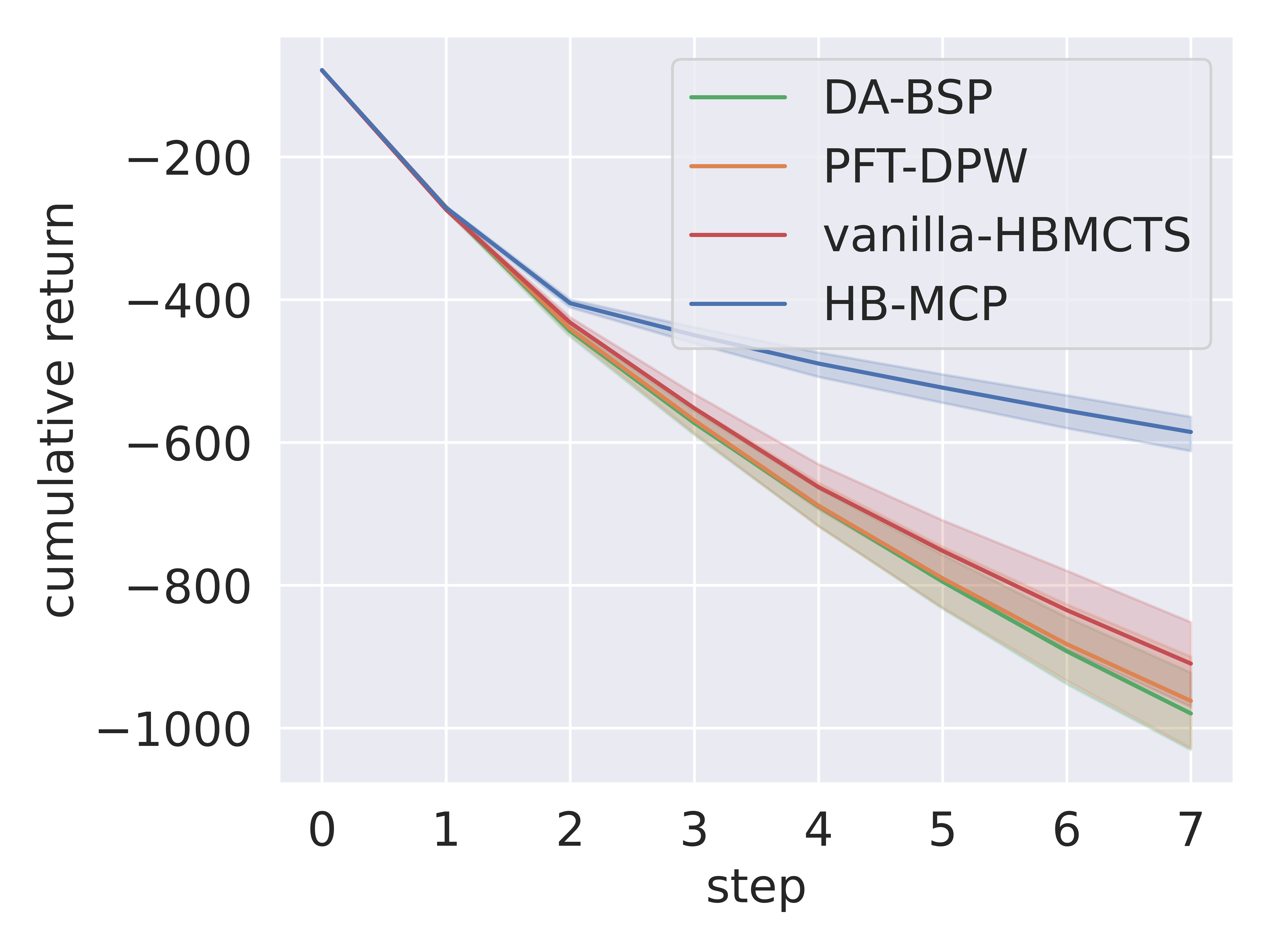
(a) cumulative return

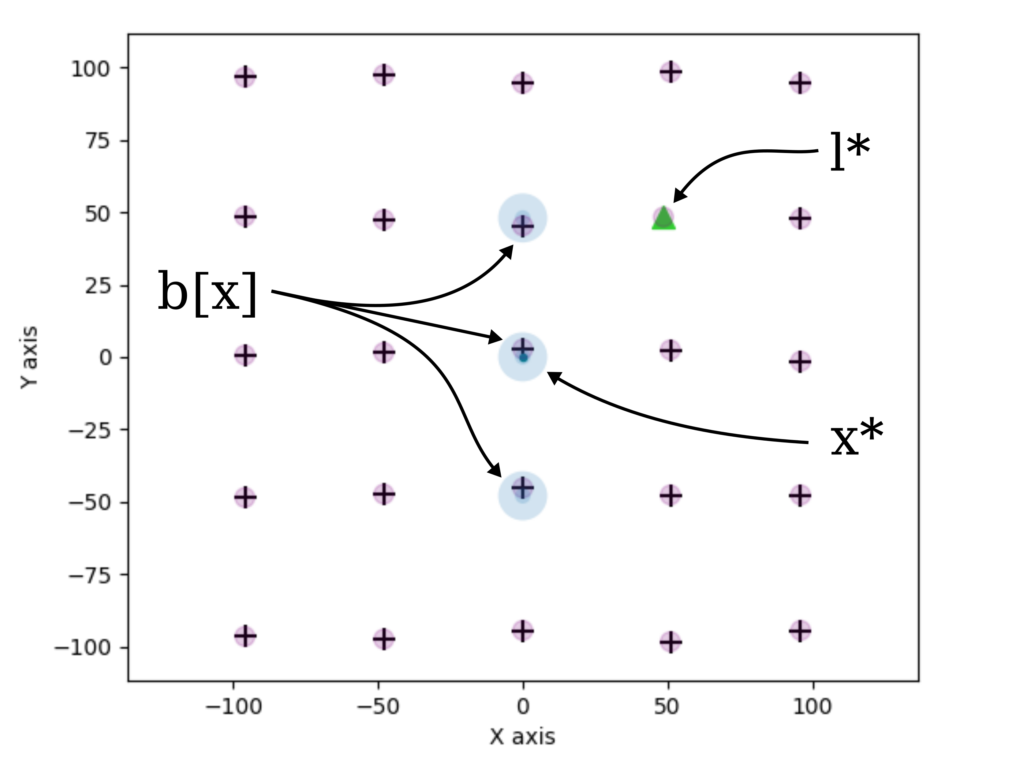
(b) initial belief

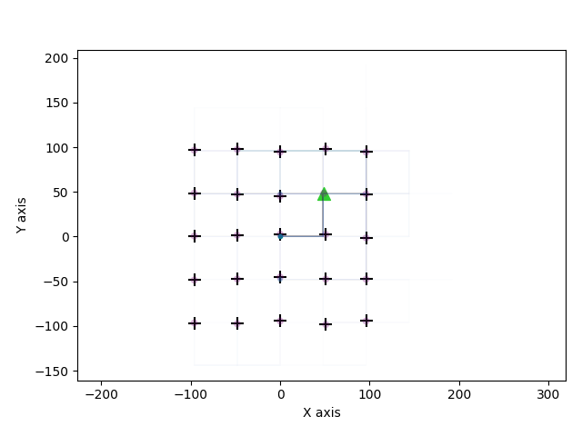
(c) trajectories

Figure 1: The goal of the agent is to minimize the uncertainty of its pose and the location of all landmarks. (a) Mean and standard deviation of the cumulative reward, over 100 trials (higher is better). (b) Illustration of the initial belief of the agent. $x^{*}$ denotes the ground truth pose of the agent. $l^{*}$ denotes a unique landmark. The agent receives as a prior three hypotheses at different locations, drawn as blue ellipses. (c) Ground-truth trajectories are visualized in transparent color, illustrated on top of the initial belief, such that multiple similar trajectories appear in a moreopaque color.

Aliased matrix. There are many ambiguous, evenly spaced landmarks around the agent, along with its ambiguous initial pose, as shown in figure 1(b). The intuitive way to reduce the uncertainty of the belief would be to first disprove wrong hypotheses, and then pass near as many landmarks as possible, such that they would be within the sensing range. The easiest way to disambiguate hypotheses would be to use the unique landmark (see figure 1(b)). It is clearly shown in figure 1(c) that the agent indeed prioritizes the unique landmark before passing near landmarks. Note that the unique landmark would only be visible (and thus provide observation) if the ground-truth position of the landmark is within the sensing range of the ground-truth pose of the agent. It can also be seen from figure 1(a) that after two macro-steps, which is the distance from the unique landmark, the descent in cumulative reward becomes less steep, and significantly outperform other algorithms.

(a) cumulative return

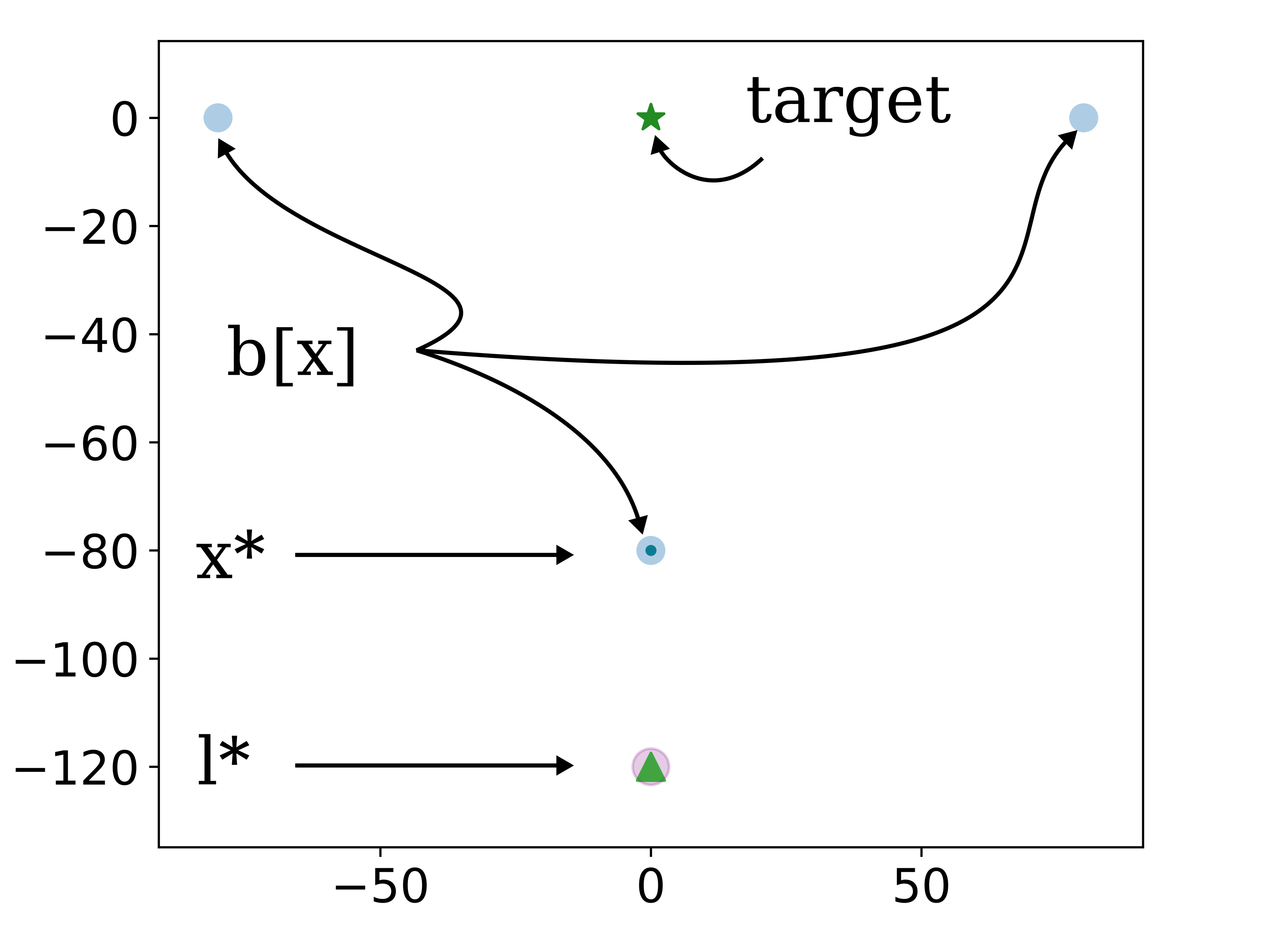
(b) initial belief

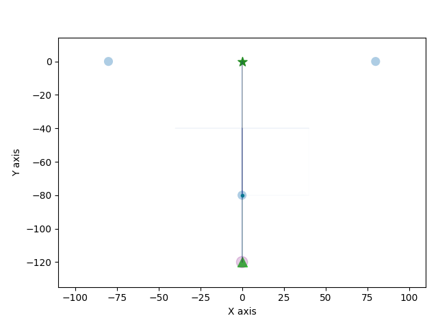
(c) trajectories

Figure 2: The goal of the agent is to reach the target location while minimizing uncertainty. (a) Mean and standard deviation of the cumulative reward, over 100 trials. (b) Illustration of the initial belief of the agent. $x^{*}$ denotes the ground truth pose of the agent. $l^{*}$ denotes a unique landmark. The agent receives as a prior three hypotheses at different locations. (c) Ground-truth trajectories are visualized in transparent color, illustrated on top of the initial belief, such that multiple similar trajectories appear in a moreopaque color.

Goal reaching. As shown in 2(c), most of the trajectories performed by the agent only walk through a simple straight line. Due to the multi-modal hypotheses, the agent first prioritizes the unique landmark (figure 2(b)), which practically disambiguates wrong hypotheses due to their large distance from the unique landmark. Then, the agent chooses to reach the goal region to maximize the cumulative reward.

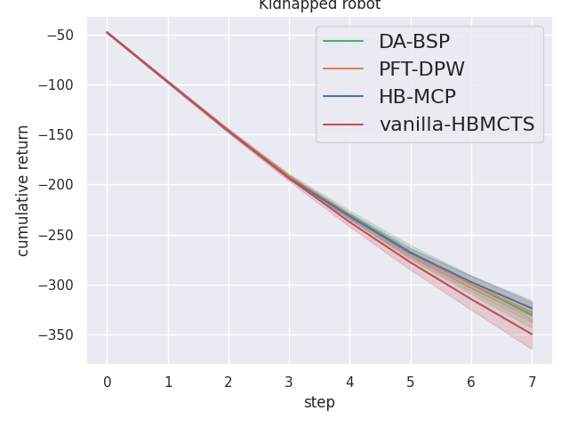
(a) cumulative return

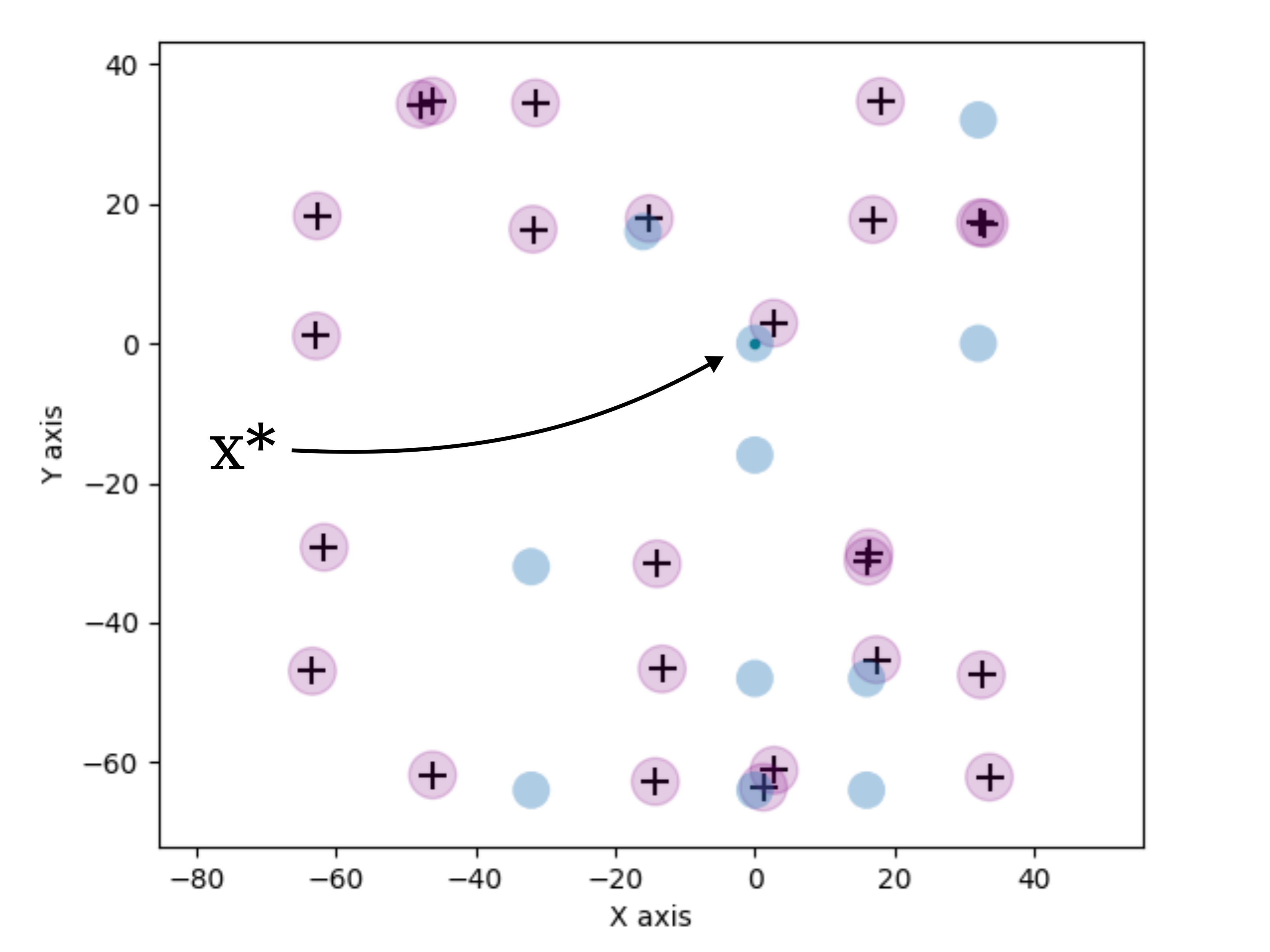
(b) initial belief

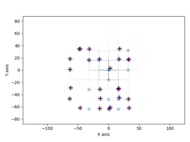
(c) trajectories

Figure 3: The goal of the agent is to minimize the uncertainty of its pose. (a) Mean and standard deviation of the cumulative reward, over 100 trials. (b) Illustration of the initial belief of the agent, blue circles illustrate conditional beliefs, crosses denote landmarks. (c) Ground-truth trajectories are visualized in transparent color, illustrated on top of the initial belief, such that multiple similar trajectories appear in a moreopaque color.

Kidnapped robot. The trajectories shown in figure 3(c) do not show a strong preference to any direction. Note that the environment is highly aliased, and there is no unique landmark where the agent may reach to easily disprove wrong hypotheses. Similar results were obtained through all solvers (figure 3(a)). Although all landmarks look alike, disambiguation may occur by utilizing the pattern of the scattered landmarks. However, such disambiguation may require a long planning horizon which was out of reach for our non-optimized planner.

Hyperparameter	Description	Default Value
$c$	UCB exploration constant	40
$N_{x}$	Number of state particles per belief node	200
$T_{m}$	Time limit per planning step (in seconds)	20 / 40
$\mathcal{T}$	Lookahead horizon	8
$k_{o}$	Observation double progressive widening multiplicative	2.0
$\alpha_{o}$	Observation double progressive widening exponent	0.014

Table 1: Hyperparameters for HB-MCP (ours), vanilla-HB-MCTS and PFT-DPW algorithm. ¹ indicates the planning time for Goal reaching and Kidnapped robot scenarios. ² indicates the planning time for Aliased matrix scenario.

	Aliased matrix	Goal reaching	Kidnapped robot
HB-MCP (ours)	-585.2	-716.8	-323.7
vanilla-HB-MCTS	-909.6	-939.4	-349.5
PFT-DPW	-961.8	-1009.8	-327.8
DA-BSP	-979.5	-931.5	-330.4

Table 2: Comparison of algorithm performances on different scenarios. Results are based on a simulation study with 100 trials per scenario and algorithm.

References

[1]
M. Barenboim, M. Shienman, and V. Indelman, “Monte carlo planning in hybrid
belief pomdps,” IEEE Robotics and Automation Letters (RA-L),
submitted.
[2]
Z. Sunberg and M. Kochenderfer, “Online algorithms for pomdps with continuous
state, action, and observation spaces,” in Proceedings of the
International Conference on Automated Planning and Scheduling, vol. 28,
no. 1, 2018.