Revisiting Attention Weights as Explanations from an Information Theoretic Perspective

Abstract

Attention mechanisms have recently demonstrated impressive performance on a range of NLP tasks, and attention scores are often used as a proxy for model explainability. However, there is a debate on whether attention weights can, in fact, be used to identify the most important inputs to a model. We approach this question from an information theoretic perspective by measuring the mutual information between the model output and the hidden states. From extensive experiments, we draw the following conclusions: (i) Additive and Deep attention mechanisms are likely to be better at preserving the information between the hidden states and the model output (compared to Scaled Dot-product); (ii) ablation studies indicate that Additive attention can actively learn to explain the importance of its input hidden representations; (iii) when attention values are nearly the same, the rank order of attention values is not consistent with the rank order of the mutual information (iv) Using Gumbel-Softmax with a temperature lower than one, tends to produce a more skewed attention score distribution compared to softmax and hence is a better choice for explainable design; (v) some building blocks are better at preserving the correlation between the ordered list of mutual information and attention weights order (for eg. the combination of BiLSTM encoder and Additive attention). Our findings indicate that attention mechanisms do have the potential to function as a shortcut to model explanations when they are carefully combined with other model elements.

1 Introduction

Attention mechanisms have been used as a way to provide insight into the workings of deep learning models in several tasks [25, 4, 11, 12, 18] However, there is a debate about whether attention weights are a good proxy for explanations. In [5], the authors argue that the attention weights cannot be used for explanations by (1) showing the inconsistency between the attention weights and other feature-importance measures; (2) showing an alternative attention distribution can yield similar results to those obtained by the original model. However, in [24], it was shown that the attention weights obtained from the original model are much more effective at prediction than the manually input decision-imitative attention weights. This result, while weakening the claim that “attention is not explanation”, does not suggest that the attention mechanism is explanation.

In this work, we continue to research this question, but from an information theoretic perspective. We focus on the encoder-attention-decoder structure [1], which is one of the most common structures used in NLP tasks. Our analysis is different from those of [5, 24], where the explainability of attention weights with respect to (w.r.t) the model inputs (e.g., token sequences) is studied. We focus on the attention mechanism itself and aim to evaluate if the attention mechanism can explain the importance of its inputs. Specifically, we look into representations of individual tokens, which are the input to the attention layer and the model output, and explore the ability of attention weights to serve as a proxy for the explanation.

Our goal is to understand what role the attention mechanism plays in the encoder-attention-decoder framework from an information theoretic perspective. We ask the following questions: (1) how does the choice of the types of attention mechanism affect the amount of information that is encoded in the representations, which are inputs to the attention layer? (2) Can we identify specific combinations of "encoders" and attention mechanisms that are best suited to build explainable models? (3) Can attention mechanisms learn to assign higher attention values to representations that have higher mutual information (MI) w.r.t the model output?

To answer these questions, we start by estimating the MI between the model output and the inputs of the attention layer (e.g., representations of the tokens). The measured MI is representative of the amount of information about the outputs that is presented in each representation. By rank ordering the attention values and observing the variation of the corresponding MI values, we can estimate how closely the attention values track the information contained in the output values.

By measuring these relations across various types of encoder and attention mechanisms, we find that the attention scores obtained from Additive attention [1] are the best proxy for explaining a model compared to Scaled Dot-Product [21] and Deep [14] attention mechanisms. Additionally, we find that the combination of the BiLSTM encoder and Additive attention [1] mechanism consistently yields attention score ranks that are positively correlated to the ranking of MI between the output and the representations.

Then, based on the combination of BiLSTM and Additive attention mechanism, we investigate the third question, namely, is the attention mechanism able to learn to assign higher attention scores to the representations with higher MI. We find that the Additive attention mechanism can indeed actively learn to assign higher scores to the input representations that contain more information about the output. Moreover, as in [24], we conduct an adversarial distribution study to assess the robustness of attention scores to such manipulations. Our results show that, even under an adversarial manipulations of the attention distribution (designed to produce similar output distribution while maximizing the Kullbach-Leibler (KL) distance from the the original distribution of the attentions), the attention weights still track the hidden representations with high MI. These findings are encouraging that the attention mechanism has the potential to be used as a proxy for the model explanation. We summarize our contributions as follows:

• We analyze the workings of the attention mechanism from an information-theoretic perspective;

• We conduct extensive experiments across various types of encoder and attention mechanisms and find that the combination of BiLSTM and Additive attention can be used to construct explainable models, since higher attention scores in this combination are always assigned to the representations that have the highest mutual information values with the model output.

• We find that attention scores are unable to track informative inputs when their values are close. We also find that increasing the differences in attention values can improve their explainability in most cases.

• We find that the attention mechanisms can actively learn the important input representations;

• We conduct adversarial distribution analysis on attention weights and show that the attention modules are robust to such manipulations.

2 Preliminary

In this work, we focus on NLP tasks and follow a general encoder-attention-decoder structure. We denote the model inputs $x\in\mathbb{R}^{T\times|\mathcal{V}|}$ as a sequence of tokens with length $T$, where each token is represented as a one-hot vector indicating a specific word in the vocabulary set $\mathcal{V}$. Firstly, the inputs are passed through the embedding layer to obtain a dense representation $x_{e}\in\mathbb{R}^{T\times d}$, where $d$ is the embedding size. Then the embedded inputs are fed into the encoder (Enc) to produce $T$ hidden representations: $\mathbf{h}=\textbf{Enc}(x_{e})\in\mathbb{R}^{T\times l}$, where $l$ is the size of the representation vector. Next, a set of $T$ attention scores $\hat{a}\in\mathbb{R}^{T}$ for the hidden representations $\mathbf{h}$ is calculated as: $\hat{a}=\textbf{Attn}(\mathbf{h},Q)$ with some attention mechanisms Attn. Here, $Q\in\mathbb{R}^{l}$ is the query vector in some task to obtain a query-related attention. Then, a context vector $c\in\mathbb{R}^{l}$ is calculated as the attention-weighted sum of all hidden representations: $c=\sum^{T}_{i=1}a_{i}h_{i}$, where $h_{i}$ is the $i^{th}$ hidden representation in $\mathbf{h}$ and $a_{i}\in\hat{a}$ is the attention score for $h_{i}$. Finally, the decoder ($\mathbf{Dec}$) processes this context vector and produces the final output of the model $\hat{y}=\mathbf{Dec}(c)\in\mathbb{R}^{o}$, where $o$ denotes the size of the output and varies depending on the specific tasks for which the model is deployed (e.g. for binary classification $o=1$ and for multi-class classification $o>1$ ).

In the following sections, we will introduce the types of attention mechanisms (Attn), encoders (Enc), and decoders (Dec) that we consider.

2.1 Attention Mechanisms

We consider three types of attention mechanisms for the $\mathbf{Attn}$ function described above: Scaled Dot-Product [21] (denoted as Dot in the rest of paper), Additive [1], and Deep [14]. For the hidden representations $\mathbf{h}$, query vector $Q$ and softmax function $\sigma$, the Dot attention scores are calculated as:

$$\mathbf{Attn_{Dot}}(\mathbf{h},Q)=\sigma(\frac{\mathbf{h}Q}{\sqrt{m}})$$ (1)

The Additive attention is defined as:

$$\mathbf{Attn_{Add}}(\mathbf{h},Q)=\sigma(W_{1}\text{tanh}(W_{2}\mathbf{h}+W_{3}Q)),$$ (2)

where $W_{1}$, $W_{2}$ and $W_{3}$ are trainable weights. The Deep attention is defined as:

$$\mathbf{Attn_{Deep}}(\mathbf{h},Q)=\sigma(D(\textit{W}_{h}\mathbf{h}+\textit{W}_{Q}Q))$$ (3)

where $D$ is a stack of $s$ fully connected layer with RELU activation:

$$\small D(x)=W^{(s)}\text{RELU}(W^{(s-1)}\text{RELU}(...W^{(1)}\text{RELU}(x)))$$ (4)

Note that the query vector is not considered in the original design of the Deep attention mechanism. We extend it to process query vector by adding an extra weight $W_{Q}$.

The above definitions consider the existence of query vectors. It is, however, not applicable in the classification tasks considered in our experiments, where there is no query vector. We hence adjust the usage of the above attention mechanisms and make them fit well in the case where only $h$ is given. For the decoder, we simply use a fully-connected layer with an activation function applied on its output (e.g., Sigmoid or Softmax) to map the context vector $c$ to the output $\hat{y}$, since our main target is to evaluate the explainability of attention modules and not performance.

For Additive and Deep attention, we simply remove the terms that contain query vectors: we remove $W_{3}Q$ from Eq. 2 and for Dot, we use the below functions instead:

$$\mathbf{Attn_{Dot}}(\mathbf{h})=\sigma(W^{D}_{1}\mathbf{h}),$$ (5)

where $W^{D}_{1}$ is a trainable parameter.

2.2 Encoder and Decoder

In our experiments, we consider three types of encoder modules, which have different capacities for modeling contextual information. The encoders used in our experiments are Bi-LSTM, convolutional neural networks (CNN), and multi-layer perceptron (MLP). Bi-LSTM is believed to have the capacity to incorporate long-distance contextual information and can be useful for processing longer texts. CNN can only capture the information from a fixed number of neighboring elements where the number is decided by the kernel size of the convolutional layer. MLPs use an affine neural network to process each embedded input (i.e., one row in $x_{e}$) individually, and information from other time steps is never considered.

For the decoder, we simply use a fully-connected layer with an activation function applied on its output (e.g., Sigmoid or Softmax) to map the context vector $c$ to the output $\hat{y}$, since our main target is to evaluate the explainability of attention modules and not performance.

3 Information Theoretic View of Attention

In this section, we describe how we evaluate the explainability of the attention module from an information theory perspective. In Section 3.1, we describe the Information Bottleneck (IB) principle [19] and another related method and discuss their relationship to the explainability of deep models in general. Inspired by these methods, we use mutual information to understand the explainability of the attention module, as described in Section 3.2.

3.1 Background

The information bottleneck (IB) method [19] was used to understand the workings of a general deep neural network (DNN) [20]. The IB method showed that deep neural networks optimize each layer’s mutual information on input and output variables, resulting in a trade-off between compression and prediction and concludes that the optimal model transmits as much information as possible from the input $X$ to the output, $Y$, through a compressed representation (the hidden states in a DNN), $\hat{X}$, and notes that $X\rightarrow\hat{X}\rightarrow Y$ forms a Markov chain. They also showed that the stochastic gradient descent (SGD) algorithm followed the IB principle. Intuitively, the optimal $\hat{X}$ disregards all irrelevant parts in $X$ with respect to $Y$ and only keeps the relevant parts.

Recently an approach called variational information bottleneck for interpretation (VIBI) was proposed for generating model agnostic explanations [2], building on the IB theory. VIBI builds a trainable, post-hoc, model-agnostic explainer and consists of two parts: an explainer and a model approximator. The key difference between VIBI and IB is that VIBI considers instance-wise cognitive chunks (units that will act as explanations) and trades-off sufficiency with the brevity of the explanations.

Our work here is inspired by the above two approaches. In contrast to these approaches, however, we are neither trying to design an optimal DNN nor create a model agnostic explainer. We are interested in investigating the use of attention weights as a proxy for explanations since, if successful, attention weights can be a shortcut to explanations. We will do this by investigating the mutual information between the input and output of the attention modules under various settings.

3.2 Analyzing the Attention Module using Mutual Information

As mentioned earlier, previous works [5, 24] assess the explainability of attention mechanisms by linking the attention scores to the importance of each token in the input sequence.

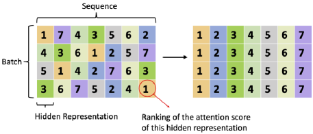
Figure 1: Diagram of collecting hidden representations for estimating mutual information. Each row represents a sequence of hidden representations of one data sample; Each cell represents one hidden representation vector where the number inside represents the rank of attention score assigned to this hidden state. On the right, it shows the collected hidden representations.

In this work, we evaluate if attention scores can be relied upon to explain the importance of the inputs to the attention mechanism. Specifically, we seek to understand how the attention scores are related to the information contained in the attention layer’s input. Here, explainability is measured by the tie-up between attention scores and the mutual information between the input to the attention layer and the model output.

The input to the attention layer is a sequence of hidden representations of the token sequence. Each hidden representation is associated with an attention score. We first rank these attention scores. We then create a vector of hidden representations formed by grouping the hidden representations for each data point with the same rank (see Fig 1). We then calculate the MI between the output and the vector of hidden representations for each rank.

This allows us to answer the question: “does the attention mechanism assign the highest attention score to the most informative (w.r.t model output) input hidden representation?”

3.2.1 Estimating Mutual Information

To estimate MI, we need to consider hidden representations that are of the same attention rank as samples from a discrete distribution. Similar to the previous works [15, 22], we discretize the representations by clustering them into a large number of clusters. Then we use cluster labels instead of the continuous representations in the MI estimator.

Specifically, we use $k$-means clustering to quantize the hidden representations and the output logits. We cluster the continuous representations into $N=50-200$ clusters. The value of $N$ is selected as the minimal value that can ensure each centroid has at least two samples. For the binary classification task, we cluster the output logits into $N=5$ clusters. For multi-class classification tasks, such as NLI and Q&A, we directly use the predicted categories.

In practice, the sequences of hidden representations are of variable length. So, we pick the $k$ hidden representations with the highest attention scores. If $k$ is too small, then many hidden representations will not be included in the computation, and we may be estimating a local maximum of the MI; If $k$ is too large, some of the samples may not have sufficient length and hence will have to be removed from consideration when calculating the MI estimate. Hence the estimate could be noisy. Thus, we compromise on selecting $k$ as the minimum value that satisfies either of the following criteria: 10-th percentile of sequence length or the critical value of $k$ such that attention weights in 80% of the selected hidden representations are larger than $10^{-5}$. The later criteria is based on the facts that extreme small attention weights will greatly reduce the gradients propagated to the corresponding hidden representation and hence is less likely to be “informative”.

Thus, we compromise on selecting $k$ so that the attention weights of 80% of the $k^{th}$ hidden representations are larger than $10^{-5}$. The reason for this is that the hidden representations with extremely low attention weights are rarely updated to minimize the training error (due to small gradients) and hence have less likely to be informative.

4 Tasks and Datasets

We follow the NLP tasks and datasets that are considered in  [5] and their implementation for data pre-processing and model training. The NLP tasks include binary text classification, natural language inference and question answering. The statistics of all datasets are described in Table 1

Dataset	|V|	Avg. length	$\#$ Train	$\#$ Test	Performance (BiLSTM)
SST	16175	19	3034 / 3321	863 / 862	0.82
IMDB	13916	179	12500 / 12500	2184 / 2172	0.90
ADR Tweets	8686	20	14446 / 1939	3636 / 487	0.86
20 Newsgroups	8853	115	716 / 710	151 / 183	0.92
AG News	14752	36	30000 / 30000	1900 / 1900	0.96
Diabetes (MIMIC)	22316	1858	6381 / 1353	1295 / 319	0.89
Anemia (MIMIC)	19743	2188	1847 / 3251	460 / 802	0.91
bAbI (Task 1 / 2 / 3)	40	8 / 67 / 421	10000	1000	0.98 / 0.74 / 0.57
SNLI	20982	14	182764 / 183187 / 183416	3219 / 3237 / 3368	0.78

Table 1: Dataset statistics. Generally, we follow the train-test split method used in  [5]. For train and test size, the number of samples in each class is listed and separated by “/”. The classes are seperated as 0/1 for binary classification (top), and 0 / 1 / 2 for NLI (bottom). Average length is in tokens. We report the accuracy of the BiLSTM encoder + Additive attention mechanism. We note that results using CNN and MLP encoders are comparable for classification though markedly worse for QA tasks.

Binary Text Classification

We use a total of 7 datasets for the text classification task. They include two sentiment analysis datasets from Standford Sentiment Treebank (SST) [17] and the IMDB Movie Reviews [10], where the target prediction is a binary variable to indicating positivity or negativity. The other five datasets include the Twitter Adverse Drug Reaction dataset [13], where the task is to identify if adverse drug reactions are mentioned in a tweet; 20 Newsgroups dataset, where the task is to distinguish if a news article is describing hockey or baseball; AG News Corpus dataset, where the task is to discriminate between world and business articles; Anemia and Diabetes datasets from MIMIC ICD9 [7], where the tasks are to determine the type of Anemia (Chronic or Acute) and whether a patient is diabetic or not, respectively.

Natural Language Inference:

We consider the SNLI [3] dataset, where each sample contains a pair of sentences and a classification label to indicate the textual entailment within the sentence pair. There are three possible classification labels: entailment, contradiction, and neutral.

Question Answering

We use bAbI [23] dataset. Each sample in bAbI contains a triplet of paragraph-question-answer, where the answer is one of the anonymized entities in the paragraph. The task requires the model to select an answer from the paragraph given the question. Specifically, we treat each of the three datasets presented in the original bAbI datasets as an individual dataset. The differences between them are the number (from 1 to 3) of supporting statements (coherent with each other) for answering a question.

5 Results

We now investigate if the attention scores are related to the amounts of information that the hidden states preserve about the model output using Kendall correlation between the ranks of mutual information and attention scores.

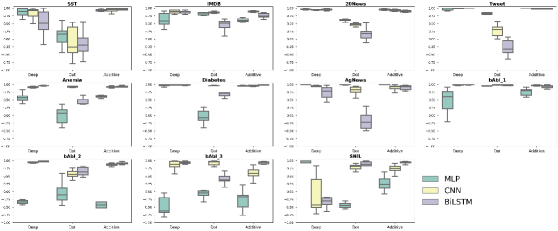
Figure 2: Box plots of weighted Kendall correlation between attention and mutual information for the representations (y-axis). X-axis denotes the types of the attention mechanism; Encoder variants are denoted by different colors.

Kendall correlation [8, 16] is a statistic used to measure the ordinal association between two measured quantities. If the hidden representations with the highest attention scores also correspond to the highest value of mutual information between the input to the attention mechanism and the model output, we can conclude that there is a strong correlation between the attention scores and the mutual information. We measure Kendall correlation $\tau$ between $(m_{1},...,m_{k})$ and $(\bar{\hat{a}}_{1},...,\bar{\hat{a}}_{k})$, where $\bar{\hat{a}}_{i}$ is the mean of the $i^{th}$ largest attention scores across test dataset and $m_{i}$ is MI between the hidden representation corresponding to the $i^{th}$ value in the ordered attention score and the output. The highest value of $\tau$ is 1, and occurs when the rank orders of the two quantities are the same (i.e., most attended hidden states are the most informative about the output).

We use the weighted Kendall correlation [16] with the attention scores (i.e., $\bar{\hat{a}}_{i}$) as the weights. We do this to ensure that the mismatches at the high end (higher-ranked values) of the vector are penalized more than mismatches at the lower end of the vector.

Figure 2 shows box plots of weighted Kendall correlation of 10 runs for each combination of encoder and attention mechanism. It illustrates that Deep attention and Additive attention achieves comparable results across all types of encoder on most classification datasets (except MLP encoder on Anemia dataset). For Q&A and NLI tasks, we observe that $\tau$ values drop for all datasets, with the drops being more significant when the MLP encoder is used. The Dot attention mechanism shows much lower correlations compared to Deep and Additive attention mechanisms on all datasets and all types of encoders.

The average value of $\tau$ (across all datasets and all encoder types over 10 runs) for the Additive, Deep and Dot attentions are $0.80$, $0.74$, and $0.45$, respectively. This indicates that among the three attention mechanisms, Additive attention mechanism is the best at indicating the most informative hidden states. We also find that the combination of Additive attention and BiLSTM has the best $\tau$ most of the time, with an average of $0.92$. The $\tau$ values for CNN and Additive attention, CNN and Deep attention and BiLSTM and Deep attention are also high at $0.88$, $0.83$ and $0.80$ respectively.

In the interest of reproducibility, we report the model accuracy of the BiLSTM and Additive attention, averaged over $10$ different initialization seeds. For each random seed, we run the model 10 times. The results show negligible differences in model performance where the average absolute difference on Kendall $\tau$ is 0.02 and the maximum difference is 0.05 on AG News Corpus.

5.1 Ablation

In this section, we address the question: can the attention module learn the highest mutual information representations? We answer this question via an ablation study. In the Fix Rep setting, we study the effect of the attention mechanism by fixing the representations that are input to the attention module and train the attention mechanism from scratch. In the Fix Attn setting, we fix the attention scores, and train both the encoder and decoder from scratch to figure out if the BiLSTM would somehow “move” the informative representations to the positions with high attention scores. In this section, we focus on the setting of BiLSTM + Additive because this setting shows the most promising results so far.

Table 2: Differences in weighted Kendall correlation between normally trained BiLSTM+Additive and the variants under special settings (Fix Rep and Fix Attn). $\Delta\tau=\tau_{\text{normal}}-\tau_{\text{special settings}}$.

Dataset	$\Delta\tau$
	Fixed Attn	Fixed Rep
SST	0.71	-0.02
IMDB	0.16	-0.01
AG News.	0.75	-0.07
ADR Tweets.	0.30	0.00
20News	1.32	-0.07
Anemia	0.97	-0.01
Diabetes	1.23	-0.01
bAbI 1	1.70	-0.02
bAbI 2	1.22	-0.06
bAbI 3	0.66	0.00
SNLI	0.07	-0.05

The changes in weighted Kendall correlation between the normally trained BiLSTM+Additive and models trained in the above settings are reported in Table 2. From this table, we notice that there is a large drop in the Kendall correlation in the Fixed Attn setting, whereas there is no drop in the Kendall correlations in the Fix Rep setting. Since the Kendall correlations were near perfect (i.e $\tau\sim 1$) for the normally trained BiLSTM+Additive, this implies that the rankings of the MI and attention scores do not correlate well when the attention values are forced to a constant. This implies that the additive attention mechanism plays a vital role in tracking the representations with highest MI. Moreover, in the Fix Rep, we observe that the resultant weighted Kendall correlation either increase or remain the same. This indicates that BiLSTM does not add to the ability of keeping the correlation between MI and attention scores. This indicates that, under the same tasks, datasets and training objective functions, the additive attention modules learn to assign higher attention scores to the representations with higher MI w.r.t the output.

5.2 Adversarial Model

Both [5, 24] claim that the premise of ”attention is explanation" is that alternative attention weights ought to yield corresponding changes in output. They demonstrated that there exists an adversarial attention distribution that is very different from the distribution of the attention weights in the normally trained models that still yields similar output distribution. In this section, we repeat our experiments in the Section 3.2 under adversarial settings to evaluate if the conclusions change.

We consider the adversarial model proposed in [24] as the scenario considered in [5] is less realistic (a detailed discussion can be found in Section 2.1 of [24]). Given the base model $M_{b}$, Authors of [24] train a model $M_{a}$ whose explicit goal is to provide similar prediction scores for each instance while distancing its attention distributions from those of $M_{b}$. The loss formula is defined as:

$$\mathcal{L}(M_{a},M_{b})=\sum_{i=0}^{n}\text{TVD}(\hat{y}^{i}_{a}-\hat{y}^{i}_{b})-\lambda\text{KL}(\hat{a}^{i}_{a}-\hat{a}^{i}_{b}),$$ (6)

where $\hat{y}^{i}$ and $\hat{a}^{i}$ denote predictions and attention distributions for the $i^{th}$ sample, respectively and $\lambda$ is a hyperparameter. TVD stands for total variation distance, and KL stands for the Kullback–Leibler Divergence. In [24], the above adversarial model is only tested on the classification datasets. To show how well the adversarial models are trained, we report the highest F1 scores of models, the divergence of attention distributions from the base, divergence of output distribution between the base and adversarial as well as their $\lambda$ setting, in Table 3. In our work, we do the same. We also tried to extend their method of adversarial distribution generation for other datasets (Q&A and NLI tasks), but it appears that this model does not work to produce different adversarial distributions for these tasks. Hence we test against adversarial distributions for classification tasks.

Table 3: Evaluation and settings of the adversarial models. We use Jensen Shannon divergence (JSD) for measuring the divergence of output distributions.

Dataset	$\lambda$	Accuracy ($\uparrow$)	TVD ($\downarrow$)	JSD ($\uparrow$)
SST	5.25e-4	0.82	0.036	0.316
IMDB	8e-4	0.90	0.021	0.482
AG News.	5e-4	0.96	0.009	0.664
ADR Tweets.	5e-4	0.87	0.001	0.194
20News	5e-4	0.90	0.037	0.391
Anemia	5e-4	0.91	0.020	0.384
Diabetes	2e-4	0.89	0.021	0.464

The changes in weighted Kendall correlation between the normally trained BiLSTM+Additive and models trained in the adversarial setting are reported in Table 4. We notice that there is not a big drop in the value of $\tau$. This implies that the attention values are still tied to the mutual information between the representation and the output.

Table 4: Differences in weighted Kendall correlation between normally trained BiLSTM+Additive and its adversarially trained counterparts. $\Delta\tau=\tau_{\text{normal}}-\tau_{\text{adv}}$.

Dataset	$\Delta\tau$
SST	0.04
IMDB	0.08
AG News.	0.05
ADR Tweets.	0.02
20News	0.09
Anemia	0.02
Diabetes	0.05

5.3 Towards Designing Explainable Attention Networks

We are interested to know when the attention weights lose their validity to indicate the most important hidden representations. We find that the attention weights for the models with lower Kendall $\tau$ tend to be more uniformly distributed than the models that achieve higher Kendall $\tau$. The finding shows that the attention weights are not accurate indicators of the quantity of information when attention weights are close. This finding would caution against using attention values as explanation without considering their relative magnitude.

To further validate this hypothesis, we intervene in the attention scores generation process so that the differences between attention scores are larger. To do so, we simply replace the Softmax function $\sigma$ (in Eq. 1, 2, 3) in the attention layer with the Gumbel-Softmax function [6] with a temperature of $0.8$. By setting the temperature to be smaller than one, the Gumbel-Softmax function is more likely to produce a “non-uniform” distribution than the Softmax function. Table 5 reports the statistics of changes in the Kendall $\tau$ for the models with the Gumbel-Softmax attention layers. We find that 85 out of 99 models can achieve higher or unchanged Kendall $\tau$ when the Gumbel-Softmax is used to generate diverse attention values.

These results answer our questions and suggest possible strategies to design explainable attention-based networks for NLP tasks. Moreover, we see that using Gumbel-Softmax along with Additive attention mechanisms or on classification tasks improves the Kendall $\tau$ in most cases. However, such clear pattern is relatively weak in either Deep and Dot attentions or Q&A and NLI tasks.

Table 5: Each entry reports the value of N/M, where M: total number of model settings. N: number of model settings (the combination of encoder and attention) for which the Kendall $\tau$ increases after using the Gumbel-Softmax attention layer.

Dataset	Deep	Dot	Additive	Average
Classification	20/21	19/21	20/21	59/63
Q & A	6/9	6/9	8/9	20/27
NLI	2/3	1/3	3/3	6/9
Average	28/33	25/33	31/33	85/99

6 Limitation

In order to complete the analysis of whether attention weights can indicate the most significant input to a model and hence provide an explanation of the model’s performance in terms of its most significant inputs, we would need to tie the model input to the model output. So far, the analysis presented in this paper ties the output to the input to the last hidden layer. Further analysis will be necessary before we fully understand how to use attention weights as explanations.

7 Conclusions and Future Work

In this work we make a case that attention can in fact be used as a proxy for explanation of a model, when viewed from an information theoretic perspective for NLP classification tasks. We notice that (1) the Additive and Deep attention modules are the best at tracking the representations with highest mutual information between the model output and the input to the attention unit; (2) of all models tested, BiLSTM+Additive attention seems to be the best at preserving the relationship between MI and attention weights; (3) when attention scores are more diverse, they are more representative of the importance of the inputs (4) additive attention mechanism is able to learn to assign highest attention weights to the representations with maximum MI and (5) Gumbel-Softmax is better at generating non-uniform distribution of attention values and hence better option for explainable model design for NLP classification tasks.

It would be interesting to explore more models in combination with the additive attention function. We believe this result help in constructing more explainable models using these building blocks.

Appendix A Appendix A: Model Settings and Implementations

We acknowledge that most of our implementations of model training and datasets processing are originally derived from the work of [5], where the codes can be found at https://github.com/successar/AttentionExplanation. In our experiments, we consider three types of encoder and three types of attention mechanisms. Therefore, there are nine kinds of models obtained by combining the encoders and attentions. We use the same settings for the same type of encoders.

For the BiLSTM encoder, we use one layer, bidirectional LSTM model with a hidden size of 128 for each direction. For the MLP encoder, we use a single hidden layer MLP with a hidden size of 128. For the CNN encoder, we set the sizes for the stacked filters as [1, 3, 5, 7, 15] and the number of output channels as 128.

During training, we use Adam [9] optimizer with a learning rate of 0.001 and batch size of 32. We also set the weight decay coefficient to $10^{-5}$. The training process is stopped at the best performance on the validation dataset.

References

- [1] Dzmitry Bahdanau, Kyunghyun Cho, and Yoshua Bengio. Neural machine translation by jointly learning to align and translate. arXiv preprint arXiv:1409.0473, 2014.
- [2] Seojin Bang, Pengtao Xie, Heewook Lee, Wei Wu, and Eric Xing. Explaining a black-box by using a deep variational information bottleneck approach. In Proceedings of the AAAI Conference on Artificial Intelligence, volume 35, pages 11396–11404, 2021.
- [3] Samuel R. Bowman, Gabor Angeli, Christopher Potts, and Christopher D. Manning. A large annotated corpus for learning natural language inference. In Proceedings of the 2015 Conference on Empirical Methods in Natural Language Processing, pages 632–642, Lisbon, Portugal, September 2015. Association for Computational Linguistics.
- [4] Edward Choi, Mohammad Taha Bahadori, Jimeng Sun, Joshua Kulas, Andy Schuetz, and Walter Stewart. Retain: An interpretable predictive model for healthcare using reverse time attention mechanism. Advances in neural information processing systems, 29, 2016.
- [5] Sarthak Jain and Byron C. Wallace. Attention is not Explanation. In Proceedings of the 2019 Conference of the North American Chapter of the Association for Computational Linguistics: Human Language Technologies, Volume 1 (Long and Short Papers), pages 3543–3556, Minneapolis, Minnesota, June 2019. Association for Computational Linguistics.
- [6] Eric Jang, Shixiang Gu, and Ben Poole. Categorical reparameterization with gumbel-softmax. arXiv preprint arXiv:1611.01144, 2016.
- [7] Alistair EW Johnson, Tom J Pollard, Lu Shen, Li-wei H Lehman, Mengling Feng, Mohammad Ghassemi, Benjamin Moody, Peter Szolovits, Leo Anthony Celi, and Roger G Mark. Mimic-iii, a freely accessible critical care database. Scientific data, 3(1):1–9, 2016.
- [8] Maurice G Kendall. A new measure of rank correlation. Biometrika, 30(1/2):81–93, 1938.
- [9] Diederik P Kingma and Jimmy Ba. Adam: A method for stochastic optimization. arXiv preprint arXiv:1412.6980, 2014.
- [10] Andrew L. Maas, Raymond E. Daly, Peter T. Pham, Dan Huang, Andrew Y. Ng, and Christopher Potts. Learning word vectors for sentiment analysis. In Proceedings of the 49th Annual Meeting of the Association for Computational Linguistics: Human Language Technologies, pages 142–150, Portland, Oregon, USA, June 2011. Association for Computational Linguistics.
- [11] Andre Martins and Ramon Astudillo. From softmax to sparsemax: A sparse model of attention and multi-label classification. In International conference on machine learning, pages 1614–1623. PMLR, 2016.
- [12] James Mullenbach, Sarah Wiegreffe, Jon Duke, Jimeng Sun, and Jacob Eisenstein. Explainable prediction of medical codes from clinical text. arXiv preprint arXiv:1802.05695, 2018.
- [13] Azadeh Nikfarjam, Abeed Sarker, Karen O’Connor, Rachel Ginn, and Graciela Gonzalez. Pharmacovigilance from social media: mining adverse drug reaction mentions using sequence labeling with word embedding cluster features. Journal of the American Medical Informatics Association, 22(3):671–681, 03 2015.
- [14] John Pavlopoulos, Prodromos Malakasiotis, and Ion Androutsopoulos. Deeper attention to abusive user content moderation. In Proceedings of the 2017 conference on empirical methods in natural language processing, pages 1125–1135, 2017.
- [15] Mehdi SM Sajjadi, Olivier Bachem, Mario Lucic, Olivier Bousquet, and Sylvain Gelly. Assessing generative models via precision and recall. Advances in neural information processing systems, 31, 2018.
- [16] Grace S Shieh. A weighted kendall’s tau statistic. Statistics & probability letters, 39(1):17–24, 1998.
- [17] Richard Socher, Alex Perelygin, Jean Wu, Jason Chuang, Christopher D Manning, Andrew Y Ng, and Christopher Potts. Recursive deep models for semantic compositionality over a sentiment treebank. In Proceedings of the 2013 conference on empirical methods in natural language processing, pages 1631–1642, 2013.
- [18] James Thorne, Andreas Vlachos, Christos Christodoulopoulos, and Arpit Mittal. Generating token-level explanations for natural language inference. In Proceedings of the 2019 Conference of the North American Chapter of the Association for Computational Linguistics: Human Language Technologies, Volume 1 (Long and Short Papers), pages 963–969, Minneapolis, Minnesota, June 2019. Association for Computational Linguistics.
- [19] Naftali Tishby, Fernando C Pereira, and William Bialek. The information bottleneck method. arXiv preprint physics/0004057, 2000.
- [20] Naftali Tishby and Noga Zaslavsky. Deep learning and the information bottleneck principle. In 2015 ieee information theory workshop (itw), pages 1–5. IEEE, 2015.
- [21] Ashish Vaswani, Noam Shazeer, Niki Parmar, Jakob Uszkoreit, Llion Jones, Aidan N Gomez, Łukasz Kaiser, and Illia Polosukhin. Attention is all you need. Advances in neural information processing systems, 30, 2017.
- [22] Elena Voita, Rico Sennrich, and Ivan Titov. The bottom-up evolution of representations in the transformer: A study with machine translation and language modeling objectives. arXiv preprint arXiv:1909.01380, 2019.
- [23] Jason Weston, Antoine Bordes, Sumit Chopra, Alexander M Rush, Bart Van Merriënboer, Armand Joulin, and Tomas Mikolov. Towards ai-complete question answering: A set of prerequisite toy tasks. arXiv preprint arXiv:1502.05698, 2015.
- [24] Sarah Wiegreffe and Yuval Pinter. Attention is not not explanation. In Proceedings of the 2019 Conference on Empirical Methods in Natural Language Processing and the 9th International Joint Conference on Natural Language Processing (EMNLP-IJCNLP), pages 11–20, Hong Kong, China, November 2019. Association for Computational Linguistics.
- [25] Kelvin Xu, Jimmy Ba, Ryan Kiros, Kyunghyun Cho, Aaron Courville, Ruslan Salakhudinov, Rich Zemel, and Yoshua Bengio. Show, attend and tell: Neural image caption generation with visual attention. In International conference on machine learning, pages 2048–2057. PMLR, 2015.