Simulating numerically the Krusell-Smith model with neural networks

Abstract

The celebrated Krusel-Smith growth model is an important example of a Mean Field Game with a common noise. The Mean Field Game is encoded in the master equation, a partial differential equation satisfied by the value of the game which depends on the whole distribution of states. The latter equation is therefore posed in an infinite dimensional space. This makes the numerical simulations quite challenging. However, Krusell and Smith conjectured that the value function of the game mostly depends on the state distribution through low dimensional quantities. In this paper, we wish to propose a numerical method for approximating the solutions of the master equation arising in Krusell-Smith model, and for adaptively identifying low-dimensional variables which retain an important part of the information. This new numerical framework is based on a semi-Lagrangian method and uses neural networks as an important ingredient.

1 Introduction

Krusell-Smith model, see [8], is a celebrated growth model in macroeconomics. In this model, the agents are households whose wealth and productivity are heterogeneous; they aim at maximizing some criteria involving their consumption and are bound by a borrowing limit. Krusell-Smith model differs from the previous Aiyagari-Bewley-Huggett models, see [7, 3, 5], in which the productivities of the agents are subject to some idiosynchratic noise, because it incorporates random shocks which affect the whole economy. As we shall see below, the introduction of a common noise implies a major additional difficulty and a real challenge in macroeconomics: roughly speaking, the optimal value and the optimal strategy of a single agent cannot be simply expressed in terms of his own wealth and productivity, but also depends on the distribution of states of other agents, which is a quantity in an infinite dimensional space.

However, in [8], Krusell and Smith made the important conjecture that the optimal value depends on the distribution of states mostly through a finite dimensional information, and even through a single number which is besides a nonlinear function of the latter distribution. This would mean that the optimal strategy of the agents mostly depends on a single common parameter.

The model of Krusell and Smith and the related open questions have been formulated in the language of macro-economics and were lacking of a precise mathematical formulation.

Later and independently, two authors of the present paper proposed the mathematical theory of Mean Field Games (MFGs in short), see  [12, 9, 10, 11], which aims at modelling dynamical equilibria for large populations, as it is the case, for instance, when studying deterministic or stochastic differential games (Nash equilibria) as the number of agents tends to infinity. In that case, one assumes that the rational agents are indistinguishable and individually have a negligible influence on the game, and that each individual strategy is influenced for example by some averages of quantities depending on the states (or the controls) of the other agents. In 2009, the last two authors interacted with R. Lucas who drew their attention to Krusell-Smith model and the related mathematical challenges. Although they already knew how to write, in particular for Mean Field Games with common noise, what is known nowadays as the master equation, the Krusell-Smith model was crucial in their placing this equation at the center of the theory. Indeed, the Krusell-Smith model can be seen as a Mean Field Game in which the agents interact through aggregate quantities, and that naturally leads to such a master equation, see for instance [1]. Note that the terminology master equation is inspired from statistical physics. It is a partial derivative equation (PDE in short) satisfied by the optimal value function of the considered Nash equilibrium with a continuum of agents: since, as in Krusell-Smith model, the latter optimal value depends on the whole distribution of states, the PDE is posed in an infinite dimensional space, and new mathematical notions are needed to give a meaning to the derivatives with respect to the probability measure associated with the distribution of states, see [12, 6].

The master equation has been useful to give a precise mathematical meaning to Krusell-Smith model and conjecture, but has not been used yet to check whether the latter is true; the reason for that is the infinite dimensionality of the PDE, which makes it very difficult to apply numerical methods. Even though, since 2009, many progress have been made in the mathematical anlysis of the master equation, and in using the latter for modeling in economics and other social sciences, the problem of finding efficient numerical approximations remains open.

The purpose of the present paper is to propose a numerical method for approximating the solutions of the master equation arising in Krusell-Smith model and apply it to address the above mentioned conjecture.

This new numerical framework is based on a semi-Lagrangian method (see the appendix by M. Falcone in the book by M. Bardi and I. Capuzzo-Dolcetta, [4], for semi-Lagrangian methods in the context of optimal control theory) and uses as an important ingredient neural networks to cope with high dimensionality, but also some mathematical understanding of its solution, see [2]. Besides, let us note that the fixed point formulation arising from the abovementioned numerical method might also appear easier to understand for readers who are not familiar with infinite dimensional PDEs.

Acknowledgments. This research was partially supported by the chair Finance and Sustainable Development and FiME Lab (Institut Europlace de Finance).

2 The Krusell-Smith model

We consider households (named agents hereafter) which are heterogeneous in their wealth (or capital) $x$ and productivity $y$. The dynamics of the wealth of a given agent is given by

$$dx_{t}=(r_{t}x_{t}+w_{t}y_{t}-c_{t})dt,$$

where

• $y_{t}$ is the productivity of the agent (a state variable)

• $c_{t}$ is the consumption (the control variable)

• $r_{t}$ is the interest rate (common to all agents)

• $w_{t}$ is the unitary salary (common to all agents)

The productivity $y_{t}$ is a two-state Poisson process with intensities $\lambda_{1}$ and $\lambda_{2}$, i.e. $y_{t}\in\{y_{1},y_{2}\}$ with $y_{1}<y_{2}$, and

$${\mathbb{P}}\left(y_{t+{\Delta t}}=y_{1}\right|\left.y_{t}=y_{1}\right)=1-\lambda_{1}{\Delta t}+o({\Delta t}),$$

$${\mathbb{P}}\left(y_{t+{\Delta t}}=y_{2}\right|\left.y_{t}=y_{1}\right)=\lambda_{1}{\Delta t}+o({\Delta t}),$$

$${\mathbb{P}}\left(y_{t+{\Delta t}}=y_{2}\right|\left.y_{t}=y_{2}\right)=1-\lambda_{2}{\Delta t}+o({\Delta t}),$$

$${\mathbb{P}}\left(y_{t+{\Delta t}}=y_{1}\right|\left.y_{t}=y_{2}\right)=\lambda_{2}{\Delta t}+o({\Delta t}).$$

We assume that the random processes describing the productivities of the agents are all independent (idiosynchratic noises).
Recall that a negative wealth means debts; there is a borrowing constraint: the wealth of a given household cannot be less than a given borrowing limit $\underline{x}$. In the terminology of control theory, $x_{t}\geq\underline{x}$ is a constraint on the state variable.
To determine the interest rate $r_{t}$ and the level of wages $w_{t}$, we assume that the production of the economy is described by the following Cobb-Douglas law:

$$F_{t}(X_{t},Y_{t})=A_{t}X_{t}^{\alpha}Y_{t}^{1-\alpha},$$

where

• the exponent $\alpha$ lies in $(0,1)$

• $A_{t}$ is a noisy productivity factor (the noise affects the whole economy and is independent from the productivities of the individuals)

• $X_{t}=\int_{x\geq\underline{x}}\int_{y\in\{y_{1},y_{2}\}}xdm(t,x,y)$ is the aggregate capital

• $Y_{t}=\int_{x\geq\underline{x}}\int_{y\in\{y_{1},y_{2}\}}ydm(t,x,y)$ is the aggregate labor

• The distribution $m(t,\cdot,\cdot)$ of the pairs $(x_{t},y_{t})$ is a probability measure on $[\underline{x},+\infty)\times\{y_{1},y_{2}\}$.

The level of wages $w_{t}$ and the interest rate $r_{t}$ are obtained by the equilibrium relation

$$(X_{t},Y_{t})={\rm{argmax}}\Bigl{(}F_{t}(X,Y)-(r_{t}+\delta)X-w_{t}Y\Bigr{)},$$

where $\delta$ is the rate of depreciation of the capital. This implies that

$$r_{t}=\partial_{X}F_{t}(X_{t},Y_{t})-\delta=\alpha A_{t}\frac{Y_{t}^{1-\alpha}}{X_{t}^{1-\alpha}}-\delta,\quad\quad w_{t}=\partial_{Y}F_{t}(X_{t},Y_{t})=(1-\alpha)A_{t}\frac{X_{t}^{\alpha}}{Y_{t}^{\alpha}}.$$

We assume that $A_{t}$ is a two-state Poisson process independent from the noises affecting the productivity of the agents, with intensities $\mu_{1}$ and $\mu_{2}$, i.e. i.e. $A_{t}\in\{A_{1},A_{2}\}$ with $A_{1}<A_{2}$, and

$${\mathbb{P}}\left(A_{t+{\Delta t}}=A_{1}\right|\left.A_{t}=A_{1}\right)=1-\mu_{1}{\Delta t}+o({\Delta t}),$$

$${\mathbb{P}}\left(A_{t+{\Delta t}}=A_{2}\right|\left.A_{t}=A_{1}\right)=\mu_{1}{\Delta t}+o({\Delta t}),$$

$${\mathbb{P}}\left(A_{t+{\Delta t}}=A_{2}\right|\left.A_{t}=A_{2}\right)=1-\mu_{2}{\Delta t}+o({\Delta t}),$$

$${\mathbb{P}}\left(A_{t+{\Delta t}}=A_{1}\right|\left.A_{t}=A_{2}\right)=\mu_{2}{\Delta t}+o({\Delta t}).$$

In what follows, we set

$$r_{i}(m)=\alpha A_{i}\frac{\left(\int_{x\geq\underline{x}}\int_{y\in\{y_{1},y_{2}\}}ydm(x,y)\right)^{1-\alpha}}{\left(\int_{x\geq\underline{x}}\int_{y\in\{y_{1},y_{2}\}}xdm(x,y)\right)^{1-\alpha}}-\delta,$$ (2.1)

and

$$w_{i}(m)=(1-\alpha)A_{i}\frac{\left(\int_{x\geq\underline{x}}\int_{y\in\{y_{1},y_{2}\}}xdm(x,y)\right)^{\alpha}}{\left(\int_{x\geq\underline{x}}\int_{y\in\{y_{1},y_{2}\}}ydm(x,y)\right)^{\alpha}}.$$ (2.2)

An agent solves the optimal control problem

$$\max_{\{c_{t}\}}\mathbb{E}\int_{0}^{\infty}e^{-\rho t}u(c_{t})dt\quad\hbox{subject to }\left\{\begin{array}[c]{rcl}dx_{t}&=&(w_{t}y_{t}+r_{t}x_{t}-c_{t})dt,\\ x_{t}&\geq&\underline{x},\end{array}\right.$$

where

• $\rho$ is a positive discount factor

• $u$ is a utility function, strictly increasing and strictly concave, e.g. the CRRA (constant relative risk aversion) utility:

  $$u(c)=c^{1-\gamma}/(1-\gamma),\qquad\gamma>0.$$ (2.3)

The introduction of aggregate shocks (on $A_{t}$) creates a major difficulty: in contrast with the case without aggregate uncertainty, it becomes necessary to include the entire distribution of productivity and wealth $m$ as a state variable in the optimal control problem of the individuals. This distribution is now itself a random variable and hence calendar time $t$ is no longer a sufficient statistic to describe the behavior of the system.

The aggregate state is $(A_{i},m),i=1,2$ and the individual state is $(x,y)$. The value of an individual agent when $A_{t}=A_{i}$, $i=1,2$, is $v_{i}(x,y,m)$.

The master equations satisfied by the value functions $v_{i}$ are posed in $(\underline{x},+\infty)\times\{y_{1},y_{2}\}\times{\mathbb{P}}([\underline{x},+\infty)\times\{y_{1},y_{2}\})$ and read as follows: for $i=1,2$, $\bar{\imath}=3-i$, $j=1,2$, $\bar{\jmath}=3-j$,

$$\begin{array}[c]{l}\begin{aligned} 0=&\lambda_{j}(v_{i}(x,y_{\bar{\jmath}})-v_{i}(x,y_{j}))+(w_{i}(m)y_{j}+r_{i}(m)x)\partial_{x}v_{i}(x,y_{j})+H(\partial_{x}v_{i}(x,y_{j}))\\ &-\rho v_{i}(x,y_{j})\ +\mu_{i}(v_{\bar{\imath}}(x,y_{j})-v_{i}(x,y_{j}))\\ &+\sum_{\ell=1}^{2}\int_{\hat{x}}T[m,\partial_{x}v_{i}](\hat{x},y_{\ell})\frac{\delta v_{i}}{\delta m}(x,y_{j},\hat{x},y_{\ell})d\hat{x},\end{aligned}\\ \hbox{with}\\ \begin{aligned} T[m,\partial_{x}v_{i}](\hat{x},y_{\ell})=&\lambda_{\bar{\ell}}m(\hat{x},y_{\bar{\ell}})-\lambda_{\ell}m(\hat{x},y_{\ell})-\partial_{x}\Bigl{(}(w_{i}(m)y_{\ell}+r_{i}(m)\cdot)m(\cdot,y_{\ell})\Bigr{)}(\hat{x})\\ &-\partial_{x}\Bigl{(}\partial_{p}H(\partial_{x}v_{i}(\cdot,y_{\ell}))m(\cdot,y_{\ell})\Bigr{)}(\hat{x}),\end{aligned}\end{array}$$

and

$$H(p)=\max_{c\geq 0}\left(-pc+u(c)\right).$$ (2.4)

With $u$ given by (2.3),

$$H(p)=\left\{\begin{aligned} \frac{\gamma}{1-\gamma}p^{1-\frac{1}{\gamma}},\quad\quad&\hbox{if }\quad p>0,\\ +\infty,\quad\quad&\hbox{if }\quad p\leq 0.\end{aligned}\right.$$

It may be more convenient to describe the value function by four functions on $[\underline{x},+\infty)\times{\mathbb{P}}([\underline{x},+\infty)\times\{y_{1},y_{2}\})$, namely $v_{i,j}$, $i,j=1,2$. The distribution of states is then given by two measures on $[\underline{x},+\infty)$, namely $m_{j}$, $j=1,2$. The master equation then takes the form:

$$0 = \displaystyle\lambda_{j}(v_{i,\bar{\jmath}}-v_{i,j})+(w_{i}(m)y_{j}+r_{i}(m)x)\partial_{x}v_{i,j}+H(\partial_{x}v_{i,j})$$

$$\displaystyle-\rho v_{i,j}+\mu_{i}(v_{\bar{\imath},j}-v_{i,j})+\sum_{\ell=1}^{2}\int_{\hat{x}}T_{i,\ell}[m,\partial_{x}v_{i,\ell}](\hat{x})\frac{\delta v_{i,j}}{\delta m_{\ell}}(\cdot,\hat{x})d\hat{x},$$

$$T_{i,\ell}[m,\partial_{x}v_{i,\ell}](\hat{x}) = \displaystyle\lambda_{\bar{\ell}}m_{\bar{\ell}}(\hat{x})-\lambda_{\ell}m_{\ell}(\hat{x})-\partial_{x}\Bigl{(}(w_{i}(m)y_{\ell}+r_{i}(m)\cdot)m_{\ell}\Bigr{)}(\hat{x})$$

$$\displaystyle-\partial_{x}\Bigl{(}\partial_{p}H(\partial_{x}v_{i,\ell})m_{\ell}\Bigr{)}(\hat{x}).$$

3 The semi-Lagrangian method

3.1 The dynamic programming principle applied to the Nash MFG-equilibrium

The dynamic programming principle applied to the mean field Nash equilibrium implies that for a small time step $\Delta t$,

$$v_{i,j}(x,m)\approx$$ (3.1)

$${\mathbb{E}}_{i,j}\left(\begin{array}[c]{l}\Delta tu\left(c^{*}_{i,j}(x,m)\right)+\\ e^{-\rho\Delta t}v_{i(\Delta t),j(\Delta t)}\Bigl{(}x+\Delta t(w_{i}(m)y_{j}+r_{i}(m)x-c^{*}_{i,j}(x,m)),m^{*}(\Delta t)\Bigr{)}\end{array}\right)$$

with an error of the order of $\Delta t$, where ${\mathbb{E}}_{ij}(X)$ stands to the probability of $X$ conditionned to $A(t=0)=A_{i}$ and $y(t=0)=y_{j}$, and

• $c^{*}_{i,j}(x,m)$ is the optimal consumption, associated to the optimal savings policy $s^{*}_{i,j}(x,m)=w_{i}(m)y_{j}+r_{i}(m)x-c^{*}_{i,j}(x,m)$. To take the state constraint into account, we set

  $$c^{*}_{i,j}(x,m)=\min\left(-H_{p}\left(\partial_{x}v_{i,j}(x,m)\right),\frac{x-\underline{x}}{\Delta t}+w_{i}(m)y_{j}+r_{i}(m)x\right)$$ (3.2)

• The probability measure $m^{*}(\Delta t)$ is the distribution of $(x+\Delta ts^{*}_{i,j}(x,m),y(\Delta t))$, where the optimal policy $s^{*}_{i,j}(x,m)$ is defined above.

Remark 3.1.

The dynamic programming equation (3.1) might be easier to understand than the master equation for readers who are not familiar with infinite dimensional PDEs.

Taylor expansions lead to the following discrete version of the master equation (2)-(2)

$$0= (1+\rho\Delta t)v_{i,j}(x,m)-v_{i,j}\Bigl{(}x+\Delta t(w_{i}(m)y_{j}+r_{i}(m)x-c^{*}_{i,j}(x,m)),m^{*}(\Delta t)\Bigr{)}$$ (3.3)

$$+\lambda_{j}\Delta t\left(v_{i,j}(x,m)-v_{i,\bar{\jmath}}(x,m)\right)+\mu_{i}\Delta t\left(v_{i,j}(x,m)-v_{\bar{\imath},j}(x,m)\right)$$

$$+\Delta tu\left(c^{*}_{i,j}(x,m)\right).$$

An important difficulty lies in the approximation of $m^{*}(\Delta t)$.

3.2 Approximation of $m$ and its transported version

3.2.1 Approximation of $m$

For computational purposes, we restrict ourselves to probability measures $m$ belonging to a finite dimensional space; let $d$ be the dimension of this space. The approximation of the value function $v_{i,j}$ is therefore a function defined on $[\underline{x},+\infty)\times{\mathbb{R}}^{d}$.
It is now well known that with Aiyagari and Krusell-Smith models, the distribution of capital may have a Dirac mass at the borrowing limit $\underline{x}$, see [1, 2]. Our space of discrete measures therefore contain Dirac masses at $(\underline{x},y_{j})$, $j=1,2$. The interpretation of these Dirac masses having positive coefficients is that the credit constraint is biding for a non zero percentage of the agents.
We also artificially truncate the support of the measure to the bounded interval $[\underline{x},\overline{x}]$ where $\overline{x}$ is a sufficiently large positive number. To avoid loosing any mass after the measure is transported, our space of discrete measures also contain Dirac masses at $(\overline{x},y_{j})$, $j=1,2$.
Except for these four Dirac masses, our discrete measures have piecewise constant densities on $(\underline{x},\overline{x})$, (i.e. the latter interval is partitioned into subintervals in which the density is constant, and the chosen partition depends on $j$).
Consider two subdivisions of $[\underline{x},\overline{x}]$ associated respectively to the two increasing families: $(x_{k,j})_{k=0,\dots,K_{j}}$, $j=1,2$:

$$\underline{x}=x_{0,j}<x_{1,j}<\dots<x_{K_{j},j}=\overline{x},$$

and set $h_{k,j}=x_{k+1,j}-x_{k,j}$, $j=0,\dots,K_{j}-1$. The discrete probability measures $m$ on $[\underline{x},+\infty)\times\{y_{1},y_{2}\}$ are of the form $m=\sum_{j=1}^{2}m_{j}\otimes\delta_{y=y_{j}}$, where

$$m_{j}=\alpha_{-1,j}\delta_{\underline{x}}+\sum_{k=0}^{K_{j}-1}\alpha_{k,j}{\mathds{1}}_{(x_{k,j},x_{k+1,j})}+\alpha_{K_{j},j}\delta_{\overline{x}}.$$

The $d=K_{1}+K_{2}+4$ coefficients $\alpha_{k,j}$ are nonnegative and such that

$$\alpha_{-1,1}+\alpha_{-1,2}+\sum_{j=1}^{2}\sum_{k=0}^{K_{j}-1}\alpha_{k,j}h_{k,j}+\alpha_{K_{1},1}+\alpha_{K_{2},2}=1.$$

Let ${\mathcal{P}}$ be the map the vector ${\mathbb{R}}^{d}\ni(\alpha_{-1,1},\dots,\alpha_{K_{1},1},\alpha_{-1,2},\dots,\alpha_{K_{2},2})\mapsto m$.

3.2.2 Transport of $m$

Let us set

$$\chi_{-1,j}(x,y) ={\mathds{1}}\left(x=\underline{x}\hbox{ and }y=y_{j}\right),$$ (3.4)

$$\chi_{k,j}(x,y) ={\mathds{1}}\left(x\in(x_{k,j},x_{k+1,j}]\hbox{ and }y=y_{j}\right),\quad\quad\hbox{ if }k=0,\dots,K_{j}-1,$$

$$\chi_{K_{j},j}(x,y) ={\mathds{1}}\left(x>\overline{x}\hbox{ and }y=y_{j}\right).$$

The transported measure $m^{*}$ is approximated as follows: we fix a large integer $N$ and set $x_{n,k,j}=x_{k,j}+\frac{n}{N+1}h_{k,j}$ for $n\in\{1,\dots,N\}$, $j=1,2$, and $k\in\{0,\dots,K_{j}-1\}$. Each point $x_{n,k,j}$ is transported by the optimal strategy to $\widehat{x}_{n,k,j}=x_{n,k,j}+\Delta ts^{*}_{i,j}(x_{n,k,j},m)$. We then draw $\widehat{y}_{n,k,j}$:

$${\mathbb{P}}(\widehat{y}_{n,k,j}=y_{j})=1-\lambda_{j}\Delta t,\quad\quad{\mathbb{P}}(\widehat{y}_{n,k,j}=y_{\bar{\jmath}})=\lambda_{j}\Delta t.$$

Similarly,

• $\underline{x}$ is transported by the optimal strategy to $\widehat{x}_{-1,j}=\underline{x}+\Delta ts^{*}_{i,j}(\underline{x},m)$. We draw $\widehat{y}_{-1,j}=y_{j}$ or $=y_{\bar{\jmath}}$ with respective probabilities $1-\lambda_{j}\Delta t$ and $\lambda_{j}\Delta t$

• $\overline{x}$ is transported by the optimal strategy to $\widehat{x}_{K_{j},j}=\overline{x}+\Delta ts^{*}_{i,j}(\overline{x},m)$. We draw $\widehat{y}_{K_{j},j}=y_{j}$ or $=y_{\bar{\jmath}}$ with respective probabilities $1-\lambda_{j}\Delta t$ and $\lambda_{j}\Delta t$.

The random variables $\widehat{y}_{-1,j},\;\widehat{y}_{n,k,j},\;\widehat{y}_{K_{j},j}$ are all independent.

The new probability measure $m^{*}(\Delta t)$ is given by $m^{*}(\Delta t)=\sum_{j=1}^{2}m^{*}_{j}\otimes\delta_{y=y_{j}}$, where

$$m^{*}_{j}=\alpha^{*}_{-1,j}\delta_{\underline{x}}+\sum_{k=0}^{K_{j}-1}\alpha^{*}_{k,j}{\mathds{1}}_{(x_{k,j},x_{k+1,j})}+\alpha^{*}_{K_{j},j}\delta_{\overline{x}},$$

with

$$\alpha^{*}_{k,j}=\sum_{\ell=1}^{2}\left(\begin{array}[c]{ll}&\displaystyle\alpha_{-1,\ell}\chi_{k,j}\left(\widehat{x}_{-1,\ell},\widehat{y}_{-1,\ell}\right)\\ &\displaystyle+\frac{1}{N}\sum_{p=0}^{K_{\ell}-1}\sum_{n=1}^{N}\alpha_{p,\ell}\chi_{k,j}\left(\widehat{x}_{n,p,\ell},\widehat{y}_{n,p,\ell}\right)\\ &\displaystyle+\alpha_{K_{\ell},\ell}\chi_{k,j}\left(\widehat{x}_{K_{\ell},\ell},\widehat{y}_{K_{\ell},\ell}\right)\end{array}\right).$$

3.3 Approximation of the value functions $v_{i,j}$ with neural networks and a fixed point strategy

3.3.1 Approximation of the value functions

Recall that the dimension of the space of discrete probability measures on $[\underline{x},\overline{x}]\times\{y_{1},y_{2}\}$ is $d$, and that ${\mathcal{P}}(M)$ denotes the measure associated to $M\in{\mathbb{R}}^{d}$. It may be convenient to let the approximate value functions $v_{i,j}$ actually depend on less than $1+d$ parameters. Indeed, Krusell and Smith have conjectured that the value function $v_{i,j}$ mostly depends on $m$ though the interest rate given by (2.1). We therefore introduce an integer $0\leq d_{0}<d$, and a map ${\mathcal{F}}_{i,j}:M\in{\mathbb{R}}^{d}\mapsto{\mathcal{F}}_{i,j}(M)\in{\mathbb{R}}^{d_{0}+1}$, ${\mathcal{F}}_{i,j}(M)$ being a collection of relevant parameters that can be constructed from the probability measure ${\mathcal{P}}(M)$. For example, such parameters may include the interest rate $r$ given by (2.1) and some moments of $m_{k}$, $k=1,2$.
We are going to approximate the value functions $v_{i,j}$ by means of neural networks, exploiting their capability to provide appropriate sets of parameterized functions. In our strategy, the first component of ${\mathcal{F}}_{i,j}$ is the interest rate, while the last $d_{0}$ components of ${\mathcal{F}}_{i,j}$ are not determined beforehand, but are rather found in an adaptive manner as an output of the first layer of a neural network.
Let ${\mathcal{N}}_{L,d,d_{0},d_{1},\dots,d_{L}}$ denote the chosen set of neural networks, which are real valued functions with the following characteristics: the number of layers is $L+1$, the input dimension is $d+1$ where $d$ has been introduced above, the output dimension $d_{L}$ is $1$, and the number of neurons in the hidden layers are $d_{1},\dots,d_{L-1}$. We approximate $v_{i,j}(x,{\mathcal{P}}(M))$ by $v^{{\mathcal{N}}}_{i,j}(x,{\mathcal{P}}(M))={\mathcal{V}}_{i,j}(x,{\mathcal{F}}_{i,j}(M))$, where ${\mathcal{V}}_{i,j}\in{\mathcal{N}}_{L,d,d_{0},d_{1},\dots,d_{L}}$.

3.3.2 A fixed point strategy

Before describing the fixed point strategy, let us introduce a large set ${\mathcal{S}}$ of samples $(x,M)\in[\underline{x},\overline{x}]\times{\mathbb{R}}^{d}$ such that ${\mathcal{P}}(M)$ is a probability measure on $[\underline{x},\overline{x}]\times\{y_{1},y_{2}\}$.
We consider the following fixed point iterations: $(v^{{\mathcal{N}},n}_{i,j})_{i,j}\to(v^{{\mathcal{N}},n+1}_{i,j})_{i,j}$:

• For $i=1,2$, $j=1,2$, set $v_{i,j}=v^{{\mathcal{N}},n}_{i,j}$

• For $i=1,2$, $j=1,2$,

  • For each $(x,M)\in{\mathcal{S}}$, set $m={\mathcal{P}}(M)$ and compute $c_{i,j}^{*}(x,m)$ by (3.2).

  • Find $v^{{\mathcal{N}},n+1}_{i,j}$ as the minimizer in the class of functions described above, of

    $$V\mapsto\sum_{(x,M)\in{\mathcal{S}}}\left|R_{i,j}(x,m)\right|^{2}$$

    where

    $$R_{i,j}(x,m)= (1+\rho\Delta t)V(x,m)$$

    $$-v_{i,j}\Bigl{(}x+\Delta t(w_{i}(m)y_{j}+r_{i}(m)x-c^{*}_{i,j}(x,m)),m^{*}(\Delta t)\Bigr{)}$$

    $$+\lambda_{j}\Delta t\left(v_{i,j}(x,m)-v_{i,\bar{\jmath}}(x,m)\right)$$

    $$+\mu_{i}\Delta t\left(v_{i,j}(x,m)-v_{\bar{\imath},j}(x,m)\right)+\Delta tu\left(c^{*}_{i,j}(x,m)\right)$$

    and $m^{*}(\Delta t)$ is the transported version of $m$ computed as in Subsection 3.2.

4 Some results

Hereafter, we present prelimininary numerical results. We insist that these results are only meant to illustrate the method and its outputs. We need to run more simulations, on a larger scale, to be more confident on the results and draw sound conclusions.

We took $\underline{x}=0$, $\overline{x}=30$, $y_{1}=0.7$, $y_{2}=1.4$, $\lambda_{1}=0.05$, $\lambda_{2}=0.1$, $\rho=0.15$, $\delta=0.05$, $\alpha=0.5$, $A_{1}=0.9$, $A_{2}=1.1$, $\mu_{1}=\mu_{2}=0.2$.
We used a time step of $0.25$ year.
The grids used to discretize the densities $m_{0}$ and $m_{1}$ have $d=17+10=27$ nodes. The repartition of the nodes is chosen in such a way that the grid steps are equally weighted by the measure found at the equilibrium in Aiyagari’s model with $A=1$.

.

4.1 An architecture designed for exploration

To construct approximations of thes solutions, we need to design a neural network architecture providing parameterized functions and remaining consistent with the economics of Krusell-Smith model.

Our goal is to find neural networks approximations of the value function $v_{i,j}(x,m)$ in the four different situations indexed by $i=1,2$, $j=1,2$ corresponding to productive/unproductive households, slow/fast economy i.e. $A=A_{1},A_{2}$, as a function of $x,r,{\mathcal{F}}_{1,i,j}(m),\cdots,{\mathcal{F}}_{d_{0},i,j}(m)$, where ${\mathcal{F}}_{1,i,j}(m),\cdots,$ ${\mathcal{F}}_{d_{0},i,j}(m)$ are found in adaptative way as the outputs of sublayers contained in the first layer in the neural network. In our strategy, we aim at starting with $d_{0}=0$, then increasing $d_{0}$ gradually. For example, with $d_{0}=1$, the neural network architecture is meant to find ${\mathcal{F}}_{1,i,j}(m)$ in order to complement the information given by the interest rate $r$. In the simulations reported below, the four neural networks have all the same architecture, displayed on Figure 1. Here, for brevity, we will sometimes omit the indices $i$ and $j$, i.e. we will use the notation ${\mathcal{F}}_{1}(m)$ for the output of the first sublayer contained in the first layer, see Figure 1, remembering that it will vary according to the considered situation, (productive/unproductive households , fast/slow economy).

Figure 1: The chosen architecture with $d_{0}=1$: note that in the first layer, the input $m$ is first mapped to the interest rate and to another variable ${\mathcal{F}}_{1}(m)$. Krusell and Smith conjecture that the optimal value depends on the distribution of states mostly through the interest rate, so we expect that the auxiliary variable ${\mathcal{F}}_{1}(m)$ should have a rather small importance. In the simulations reported below, the architecture is as follows: all the layers or sublayers described below, except the final one, involve the softplus activation function. The vector $(m,x)$ is processed by the first layer as follows: first $(m,x)$ is mapped to $({\mathcal{F}}_{1}(m),r,x)$ and the map ${\mathcal{F}}_{1}$ is described by a first sublayer. This means that ${\mathcal{F}}_{1}$ is the composition of an affine map from ${\mathbb{R}}^{d}$ to ${\mathbb{R}}$ with the softplus activation function. The variable ${\mathcal{F}}_{1}(m)$ is mapped to a vector in ${\mathbb{R}}^{80}$ by a second sublayer. The interest rate $r$ is mapped to a vector in ${\mathbb{R}}^{20}$ by a third sublayer. The capital $x$ is mapped to a vector in ${\mathbb{R}}^{150}$ by a fourth sublayer. The output of the first layer is therefore a vector in ${\mathbb{R}}^{d_{1}}$, $d_{1}=80+20+150=250$, obtained by concatenation. This information is then processed by a sequence of $4$ hidden fully connected layers, with dimensions $300$, $150$, $50$ and $20$.

4.1.1 The optimal savings as a function of the capital and the interest rate

In Figure 4.1.1, we fix the value ${\mathcal{F}}_{1,i,j}(m)$, and plot the contours of the optimal savings policy as a a function of the capital and the interest rate. The dotted lines correspond to negative values.

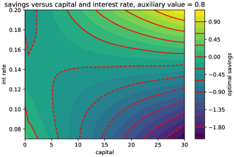
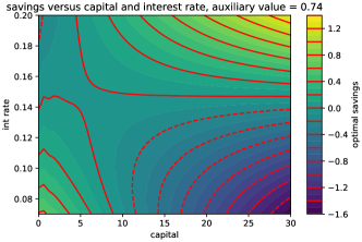
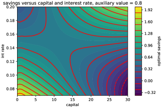
Figure 2: Top: Optimal savings for nonproductive(left) and productive(right) households when $A=A_{1}$ (slow economy) as a function of $x$ and $r$. Bottom: Optimal savings for nonproductive(left) and productive(right) households when $A=A_{2}$ (fast economy).

4.1.2 The optimal savings as a function of the capital for a given distribution $m$

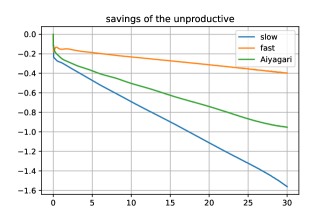
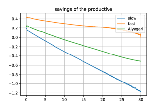
Figure 3: Optimal savings for nonproductive(left) and productive(right) households as a function of $x$ for the two values of $A$ (slow and fast economy), and the savings found by Aiyagari’s model with $A=1$. The measure $m$ is chosen as the equilibrium in Aiyagari’s model with $A=1$. Note the singular behavior in the savings of the unproductive near $x=0$; indeed, the credit constraint is biding in this situation. Note also that the savings policy found in the Aiyagari’s model with $A=1$ lies below (resp. above) the policy related to the fast (resp. slow) economy.

4.1.3 The optimal savings as a function of the interest rate and the auxiliary variable ${\mathcal{F}}_{1}(m)$

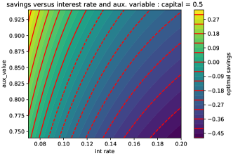
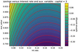
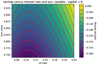
Figure 4: Optimal savings for nonproductive households when $A=A_{1}$ as a function of $r$ and the auxiliary variable ${\mathcal{F}}_{1}(m)$ for $x=0.5,\;1,\;3,\;6$.

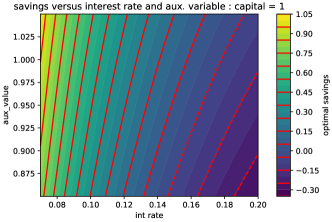
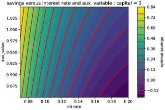
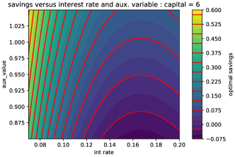
Figure 5: Optimal savings for productive households when $A=A_{1}$ as a function of $r$ and the auxiliary variable ${\mathcal{F}}_{1}(m)$ for $x=0.5,\;1,\;3,\;6$.

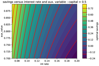
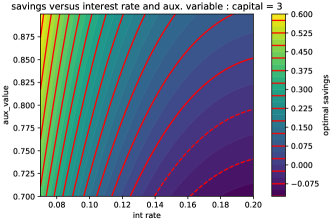
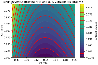
Figure 6: Optimal savings for nonproductive households when $A=A_{2}$ as a function of $r$ and the auxiliary variable ${\mathcal{F}}_{1}(m)$ for $x=0.5,\;1,\;3,\;6$.

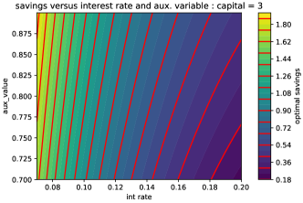
Figure 7: Optimal savings for productive households when $A=A_{2}$ as a function of $r$ and the auxiliary variable for $x=0.5,\;1,\;3,\;6$.

4.1.4 Correlation between $r$ and the auxiliary variable

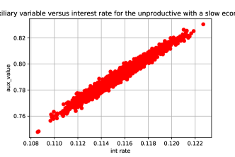
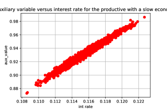
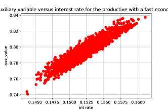
Figure 8: ${\mathcal{F}}_{1}(m)$ versus $r$ for a sample of measures $m$. Top Left: unproductive and $A=A_{1}$. Top Right: unproductive and $A=A_{2}$. Bottom Left: productive and $A=A_{1}$. Bottom Right: productive and $A=A_{2}$. We see a rather strong correlation between $r$ and ${\mathcal{F}}_{1}(m)$.

4.1.5 A tentative conclusion

In the simulations reported above, in each situation, ($i=1,2$, $j=1,2$), the approximate solution of the master equation depends on $m$ through the interest rate and an additional variable ${\mathcal{F}}_{1,i,j}(m)$, (the function ${\mathcal{F}}_{1,i,j}$ is obtained as a sublayer contained in the first layer of the neural network). While the savings strategies of the households mostly depend on the interest rate $r$ as conjectured by Krusell and Smith, the additional variables ${\mathcal{F}}_{1,i,j}(m)$ seem to bring a significant correction.

References

- [1] Y. Achdou, F. Buera, J.-M. Lasry, P.-L. Lions, and B. Moll, Partial differential equation models in macroeconomics, Philos. Trans. R. Soc. Lond. Ser. A Math. Phys. Eng. Sci., 372 (2014), pp. 20130397, 19.
- [2] Y. Achdou, J. Han, J.-M. Lasry, P.-L. Lions, and B. Moll, Income and wealth distribution in macroeconomics: a continuous-time approach, Rev. Econ. Stud., 89 (2022), pp. 45–86.
- [3] S. R. Aiyagari, Uninsured idiosyncratic risk and aggregate saving, The Quarterly Journal of Economics, 109 (1994), pp. 659–84.
- [4] M. Bardi and I. Capuzzo-Dolcetta, Optimal control and viscosity solutions of Hamilton-Jacobi-Bellman equations, Systems & Control: Foundations & Applications, Birkhäuser Boston, Inc., Boston, MA, 1997. With appendices by Maurizio Falcone and Pierpaolo Soravia.
- [5] T. Bewley, Stationary Monetary Equilibrium with a Continuum of Independently Fluctuating Consumers, in Contributions to Mathematical Economics in Honor of Gerard Debreu, W. Hildenbrand and A. Mas-Collel, eds., North-Holland, Amsterdam, 1986.
- [6] P. Cardaliaguet, F. Delarue, J.-M. Lasry, and P.-L. Lions, The master equation and the convergence problem in mean field games, vol. 201 of Annals of Mathematics Studies, Princeton University Press, Princeton, NJ, 2019.
- [7] M. Huggett, The risk-free rate in heterogeneous-agent incomplete-insurance economies, Journal of Economic Dynamics and Control, 17 (1993), pp. 953–969.
- [8] P. Krusell and A. A. Smith, Income and wealth heterogeneity in the macroeconomy, Journal of Political Economy, 106 (1998), pp. 867–896.
- [9] J.-M. Lasry and P.-L. Lions, Jeux à champ moyen. I. Le cas stationnaire, C. R. Math. Acad. Sci. Paris, 343 (2006), pp. 619–625.
- [10] J.-M. Lasry and P.-L. Lions, Jeux à champ moyen. II. Horizon fini et contrôle optimal, C. R. Math. Acad. Sci. Paris, 343 (2006), pp. 679–684.
- [11] J.-M. Lasry and P.-L. Lions, Mean field games, Jpn. J. Math., 2 (2007), pp. 229–260.
- [12] P.-L. Lions, Cours du Collège de France. https://www.college-de-france.fr/site/en-pierre-louis-lions/_course.htm, 2006-2012.