LQ Optimal Control for Power Tracking Operation of Wind Turbines

Abstract

In this paper, an approach for active power control of individual wind turbines is presented. State-of-the-art controllers typically employ separate control loops for torque and pitch control. In contrast, we use a multivariable control approach. In detail, active power control is achieved by using reference trajectories for generator speed, generator torque, and pitch angle such that a desired power demand is met if weather conditions allow. Then, a linear quadratic (LQ) optimal controller is used for reference tracking. In an OpenFAST simulation environment, the controller is compared to a state-of-the-art approach. The simulations show a similar active power tracking performance, while the LQ optimal controller results in lower mechanical wear. Moreover, the presented approach exhibits good reference tracking and by improving the reference trajectory generation further performance increases can be expected.

1 Introduction

In the last two decades, renewable energy sources have been scaled up quickly around the world (Luz et al., 2018). Apart from installing new units, an effective strategy to increase the share of renewable energy sources is to improve existing renewable generators. After hydro, wind power counts as the second most popular source of renewable energy (Child et al., 2019). For some markets, e.g., Spain or Denmark, the electricity grid relies heavily on wind power (Pullen and Sawyer, 2011). In such settings, grid operators require additional services from wind farms to ensure grid stability. In this context, active power control is an important operation mode, where a wind park does not produce as much power as possible but a given power signal is tracked. Clearly, active power control requires individual turbines to perform power tracking. Apart from power tracking performance, aspects, such as mechanical wear on wind turbine components must be considered in the controller design to decrease operation and maintenance costs (Aho et al., 2012; Kelley et al., 2007).

Traditionally, wind turbine controllers employ separate control loops for the pitch angle and the generator torque (Aho et al., 2013). Switched nonlinear single-input single-output controllers are typically used to obtain the generator torque based on the generator speed. For pitch control, a gain-scheduled proportional-integral (PI) controller has been industry standard for many years (Jonkman et al., 2009). Adaptions presented in Schlipf (2016) led to some improvements but the overall controller structure has largely remained unchanged.

For some time, multivariable control strategies, such as model predictive control or LQ optimal control, have been researched (see, e.g., Ostergaard et al., 2007; Mirzaei et al., 2013). The approach presented in Ostergaard et al. (2007), focuses on generator modeling and high wind speeds. The model predictive controller presented in Mirzaei et al. (2013) is based on a wind turbine model with five linear states based on uncertain light detection and ranging (LIDAR) measurements. In this work, we present an LQ optimal control approach which works throughout all expected wind speeds, while being based on a simple model with only one state. The model assumes a rigid gearbox with no damping to link rotor and generator. We show that the LQ optimal controller obtained from the simplified model performs better than state-of-the-art controllers. In a numerical case study, the developed controller is benchmarked and evaluated in an OpenFAST simulation environment (Jonkman et al., 2022) along with a baseline controller. This includes an analysis of dynamical behavior as well as an investigation of mechanical wear.

The remainder of this paper is organized as follows. The wind turbine model is provided in Section 2. In Section 3, a state-of-the-art controller is introduced. In Section 4, our LQ optimal control scheme is proposed. In Section 5, a case study that compares state-of-the-art with our multivariable controller is presented. Finally, in Section 6, conclusions and suggestions for future work are provided.

1.1 Notation

The set of real numbers is denoted by $\mathbb{R}$ and the set of positive real numbers by $\mathbb{R}^{+}$. The set of nonnegative real numbers is denoted by $\mathbb{R}^{+}_{0}$, while $\mathbb{N}$ denotes the positive integers. The $\mathop{\ThisStyle{\raisebox{-2.4pt}{\kern 0.5pt\LMpt\scaleto{ \leavevmode\hbox to428.34pt{\vbox to428.34pt{\text{[drawing]}}}}{2.25\LMex}\kern 0.5pt\LMpt}}}$ operator applies a saturation, i.e.,

$$y=\mathop{\ThisStyle{\raisebox{-2.4pt}{\kern 0.5pt\LMpt\scaleto{ \leavevmode\hbox to428.34pt{\vbox to428.34pt{\text{[drawing]}}}}{2.25\LMex}\kern 0.5pt\LMpt}}}_{\underline{x}}^{\overline{x}}x=\begin{cases}\underline{x},&\text{if }x\leq\underline{x},\\ \overline{x},&\text{if }x\geq\overline{x},\\ x,&\text{else},\end{cases}$$ (1)

where $x\in\mathbb{R}$ is being saturated by the upper bound $\overline{x}\in\mathbb{R}$ and the lower bound $\underline{x}\in\mathbb{R}$, with $\underline{x}<\overline{x}$, such that $y\in[\underline{x},\overline{x}]$. The $\operatorname{LUT}$ (lookup table) operator maps a given input using linear interpolation into the codomain based on underlying data points. Finally, $I_{j}$, with $j\in\mathbb{N}$, represents the $j$-by-$j$ identity matrix and $0_{2}=\begin{bmatrix}0&0\end{bmatrix}^{T}$.

2 Model

The considered wind turbine model is composed of three parts: rotor aerodynamics, drive train, and generator (see Aho et al., 2012; Boersma et al., 2017). First, the rotor blades convert wind into rotational power. Then, the drive train converts slow rotations into fast ones. Finally, the generator converts mechanical into electrical power. Yaw control is not considered because we assume a constant wind direction. In what follows, we introduce this model in more detail and derive a linearized version of the overall dynamics.

2.1 Rotor Aerodynamics

The wind that passes through the round rotor swept area of a wind turbine with radius $r\in\mathbb{R}^{+}$ has a power of

$$P_{wind}(t)=\frac{\rho}{2}\pi r^{2}V(t)^{3},$$ (2)

where $\rho\in\mathbb{R}^{+}$ and $V(t)\in\mathbb{R}^{+}$ denote air density and wind speed at time $t$, respectively. A wind turbine can only convert a certain proportion of the wind power into rotational power $P_{r}(t)\in\mathbb{R}^{+}$. The power coefficient

$$C_{p}\big{(}\lambda(t),\theta(t)\big{)}=\frac{P_{r}(t)}{P_{wind}(t)},$$ (3)

allows to describe this value. It is a function of the pitch angle $\theta(t)\in\mathbb{R}$ and the tip-speed ratio

$$\lambda(t)=r\frac{\omega_{r}(t)}{V(t)},$$ (4)

where $\omega_{r}(t)\in\mathbb{R}^{+}$ denotes the angular velocity of the rotor. Combining (2) and (3), the power extracted by the rotor can be written as

$$P_{r}(t)=\frac{\rho}{2}\pi r^{2}\;V(t)^{3}C_{p}(\lambda(t),\theta(t)).$$ (5)

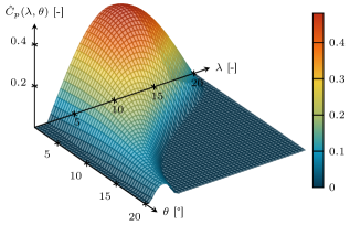
Figure 1: Approximation of power coefficient $\hat{C}_{p}\left(\lambda(t),\theta(t)\right)$ based on data from Bortolotti et al. (2019).

Then, we can obtain the aerodynamic rotor torque as

$$M_{r}(t)=\frac{P_{r}(t)}{\omega_{r}(t)}=\frac{\rho}{2}\frac{\pi r^{2}}{\omega_{r}(t)}V(t)^{3}C_{p}(\lambda(t),\theta(t)).$$ (6)

A power coefficient of $C_{p}(\cdot)=1$ corresponds to a full conversion of wind power to rotational power. However, there exists a theoretical limit for the power coefficient, i.e., $C_{p}(\cdot)<\frac{16}{27}\approx 0.59$, which holds for any rotor and blade configuration (Hansen, 2008). The power coefficient depends on various parameters, such as blade shape, material, and weight. Tools such as OpenFAST (Jonkman et al., 2022) estimate the aerodynamic torque at the rotor numerically. In recent literature (see, e.g., Merabet et al., 2011), the approximation

$$\tilde{C}_{p}=\bigg{(}\frac{a_{1}}{\lambda_{i}}+a_{2}\theta+a_{3}\bigg{)}e^{\frac{a_{4}}{\lambda_{i}}}\text{ with }\lambda_{i}=\frac{1}{\frac{1}{\lambda+a_{5}}+\frac{a_{6}}{\theta^{3}+1}},$$ (7)

is often used. However, for the wind turbine considered in this paper, an approximation of the form

$$\hat{C}_{p}(\lambda(t),\theta(t)) =\max\big{(}c_{1}+c_{2}\lambda(t)+c_{3}\theta(t)+c_{4}\lambda(t)^{2}$$

$$+c_{5}\lambda(t)\theta(t)+c_{6}\theta(t)^{2}+c_{7}\lambda(t)^{3}$$

$$+c_{8}\lambda(t)^{2}\theta(t)+c_{9}\lambda(t)\theta(t)^{2}+c_{10}\theta(t)^{3}$$

$$+c_{11}\lambda(t)^{4}+c_{12}\lambda(t)^{3}\theta(t)+c_{13}\lambda(t)^{2}\theta(t)^{2}$$

$$+c_{14}\lambda(t)\theta(t)^{3}+c_{15}\theta(t)^{4},0\big{)},$$ (8)

was found to be much more accurate. The approximation $\hat{C}_{p}(\cdot)$ is fitted from data points $(\lambda,\theta)\in\mathbb{H}\subset\mathbb{R}^{2}$. Note that the approach in Section 4 works for different approximations of $C_{p}$ - the shape from (8) is not required. In this work, the IEA $3.35\text{\,}\mathrm{MW}$ turbine is considered, hence the data points provided by Bortolotti et al. (2019) are used. A visualization for the approximated power coefficient is depicted in Figure 1.

2.2 Drive Train and Generator

We consider a rigid drive train and gearbox, i.e., $\omega(t)=N_{g}\omega_{r}(t)$, where $\omega(t)\in\mathbb{R}^{+}$ and $N_{g}\in\mathbb{R}^{+}$ denote angular generator shaft velocity and gearbox ratio, respectively. Note that wind turbines without any gearbox, as described in Wagner (2020), are modeled with $N_{g}=1$. The dynamics of the drive train are modeled by

$$J_{t}\dot{\omega}_{r}(t)=\frac{J_{t}}{N_{g}}\dot{\omega}(t)=M_{r}(t)-N_{g}\cdot M_{g}(t),$$ (9)

where $M_{g}(t)\in\mathbb{R}^{+}_{0}$ is the generator torque and ${J_{t}\in\mathbb{R}^{+}}$ the moment of inertia. The combined efficiency of drive train, generator, and power electronics is denoted by ${\eta\in\;]0,1]\subset\mathbb{R}^{+}}$. This allows us to calculate the power via

$$P_{e}(t)=\eta\omega(t)M_{g}(t).$$ (10)

2.3 State Model

Combining (4), (6), (9), and (10) results in a nonlinear state model, with state $\omega(t)$, control inputs $\begin{bmatrix}\theta(t)&M_{g}(t)\end{bmatrix}^{T}$, and uncertain input $V(t)$, with dynamics

$$\dot{\omega}(t) =f(\omega,\begin{bmatrix}\theta&M_{g}\end{bmatrix}^{T},V)$$

$$=\frac{\rho\pi r^{2}N_{g}^{2}}{2J_{t}}\frac{V(t)^{3}}{\omega(t)}\hat{C}_{p}\Big{(}\frac{r}{N_{g}}\frac{\omega(t)}{V(t)},\theta(t)\Big{)}-\frac{N_{g}^{2}}{J_{t}}M_{g}(t).$$ (11)

2.4 Linearization and Discretization

Let us assume, that system (11) exhibits a unique equilibrium $\omega^{s}$ for given $(\begin{bmatrix}\theta^{s}&M_{g}^{s}\end{bmatrix}^{T},V^{s})$ around which the model is now linearized. At the equilibrium $\dot{\omega}(t)=0$ holds. At time $t$, $\xi(t)=\omega(t)-\omega^{s}$ describes the deviation from $\omega^{s}$, $\mu(t)=\begin{bmatrix}\theta(t)&M_{g}(t)\end{bmatrix}^{T}-u^{s}$ the deviation from $u^{s}=\begin{bmatrix}\theta^{s}&M_{g}^{s}\end{bmatrix}^{T}\in\mathbb{R}^{2}$, and $\nu(t)=V(t)-V^{s}$ the deviation from $V^{s}\in\mathbb{R}^{+}$. Let us formulate the linearized state model

$$\dot{\xi}(t)=A_{\text{c}}\xi(t)+B_{\text{c}}\mu(t)+F_{\text{c}}\nu(t),$$ (12)

where

$$\begin{split}A_{\text{c}}&=\left.\frac{\partial f(\omega,\begin{bmatrix}\theta&M_{g}\end{bmatrix}^{T},V)}{\partial\omega}\right|_{\omega^{s},\big{(}\begin{bmatrix}\theta^{s}&M_{g}^{s}\end{bmatrix}^{T},V^{s}\big{)}},\end{split}$$ (13a)

$$\begin{split}B_{\text{c}}&=\begin{bmatrix}\left.\frac{\partial f(\omega,\begin{bmatrix}\theta&M_{g}\end{bmatrix}^{T},V)}{\partial\theta}\right|_{\omega^{s},\big{(}\begin{bmatrix}\theta^{s}&M_{g}^{s}\end{bmatrix}^{T},V^{s}\big{)}}\\ \left.\frac{\partial f(\omega,\begin{bmatrix}\theta&M_{g}\end{bmatrix}^{T},V)}{\partial M_{g}}\right|_{\omega^{s},\big{(}\begin{bmatrix}\theta^{s}&M_{g}^{s}\end{bmatrix}^{T},V^{s}\big{)}}\end{bmatrix}^{T},\end{split}$$ (13b)

$$\begin{split}F_{\text{c}}&=\left.\frac{\partial f(\omega,\begin{bmatrix}\theta&M_{g}\end{bmatrix}^{T},V)}{\partial V}\right|_{\omega^{s},\big{(}\begin{bmatrix}\theta^{s}&M_{g}^{s}\end{bmatrix}^{T},V^{s}\big{)}}.\end{split}$$ (13c)

For the implementation on digital controllers, a discrete time model is desirable. We derive this using the forward Euler method with sampling time $T_{s}\in\mathbb{R}^{+}$, obtaining

$$\xi(k+1)=A_{\text{d}}\xi(k)+B_{\text{d}}\mu(k)+F_{\text{d}}\nu(k),$$ (14)

where $A_{\text{d}}=1+T_{s}A_{\text{c}}$, $B_{\text{d}}=T_{s}B_{\text{c}}$, and $F_{\text{d}}=T_{s}F_{\text{c}}$.

3 Baseline Control Scheme

In this section, a state-of-the-art wind turbine controller (Bortolotti et al., 2019; Schlipf, 2016) is presented. It serves as a baseline for the comparison with the LQ optimal controller presented in Section 4.

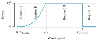
Figure 2: Wind turbine operating regions.

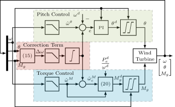
Figure 3: Closed-loop structure of the baseline controller.

Typically, a wind turbine operates in four distinct regions, as displayed in Figure 2. In Regions I and IV, the turbine is turned off due a wind speed below the cut-in wind speed $V_{\text{CutIn}}$ or above the cut-out wind speed $V_{\text{CutOut}}$. Region II is defined by maximization of output power, while the wind speed remains below the wind speed $V^{d}$ required for the desired power $P_{e}^{d}\in\mathbb{R}$. Finally, in Region III, the wind speed suffices to meet the desired power output $P_{e}^{d}$.

The presented baseline controller is capable of the power tracking operation mode, where the turbine provides a desired power below the rated power if weather conditions allow. Clearly, this is not always possible, since slow wind speeds may not provide enough power to satisfy $P_{e}^{d}$. Power tracking is achieved by computing a desired generator speed $\omega^{d}(k)$ based on the desired power $P^{d}_{e}(k)$, i.e.,

$$\omega^{d}(k)=\min\Bigg{(}\sqrt[3]{\frac{P^{d}_{e}(k)}{\eta c_{M}^{*}}},\;\omega^{\text{Rated}}\Bigg{)}.$$ (15)

Here, $c_{M}^{*}\in\mathbb{R}^{+}$ is a design parameter and $\omega^{\text{Rated}}\in\mathbb{R}^{+}$ is the rated generator speed. The first term inside the $\min$ operator can be derived from the torque controller, i.e., the last case of (20). In Figure 3, an overview of the baseline controller is shown. It can be separated into three parts: The general correction term is presented in Section 3.1. The torque control is introduced in Section 3.2 and the pitch controller is described in Section 3.3.

3.1 Correction Term

To smooth out the transition from Region II to Region III, the correction term

$$\Delta\omega(k)=c_{\theta}^{\text{GB}}\big{(}\theta(k-1)-\underline{\theta}\big{)}+c_{M}^{\text{GB}}\big{(}M_{g}(k-1)-M_{g}^{\text{Rated}}\big{)},$$ (16)

is used by the controller. Here, $c_{\theta}^{\text{GB}},c_{M}^{\text{GB}}\in\mathbb{R}^{+}$ are design parameters while $\underline{\theta},M_{g}^{\text{Rated}}\in\mathbb{R}$ denote lower pitch angle bound and rated generator torque, respectively. Before applying the correction term, a lowpass filter is used, e.g.,

$$\Delta\hat{\omega}(k)=(1-\alpha^{\text{GB}})\cdot\Delta\hat{\omega}(k-1)+\alpha^{\text{GB}}\cdot\Delta\omega(k),$$ (17)

where $\alpha^{\text{GB}}=\frac{T_{s}}{T_{\text{GB}}-T_{s}}\in[0,1]\subset\mathbb{R}^{+}_{0}$ is based on $T_{s}$ and the filter time constant $T_{\text{GB}}>2T_{s}$. The filter is initialized to $\Delta\hat{\omega}(0)=\Delta\omega(0)$. In what follows, we will describe how the baseline controller is designed based on $\omega^{d}(k)$ and $\Delta\hat{\omega}(k)$.

3.2 Torque Control

For each operating region, the generator torque $M_{g}(k)$ is computed differently. The desired generator torque $M_{g}^{d}(k)$ is computed based on a lowpass filtered generator speed measurement and the correction term. The lowpass filtered generator speed $\hat{\omega}^{M}(k)$ is derived via

$$\hat{\omega}^{M}(k)=(1-\alpha^{M})\cdot\hat{\omega}^{M}(k-1)+\alpha^{M}\cdot\omega(k),$$ (18)

where $\alpha^{M}=\frac{T_{s}}{T_{M}-T_{s}}\in[0,1]\subset\mathbb{R}^{+}_{0}$ is based on $T_{s}$ and the filter time constant $T_{M}$. The filter is initialized to $\hat{\omega}^{M}(0)=\omega(0)$. Then, the corrected generator speed

$$\hat{\omega}_{c}^{M}(k)=\hat{\omega}^{M}(k)+\mathop{\ThisStyle{\raisebox{-2.4pt}{\kern 0.5pt\LMpt\scaleto{ \leavevmode\hbox to428.34pt{\vbox to428.34pt{\text{[drawing]}}}}{2.25\LMex}\kern 0.5pt\LMpt}}}_{0}^{\infty}\Delta\hat{\omega}(k)$$ (19)

is computed and the desired generator torque is set to be

$$M_{g}^{d}(k)=\begin{cases}P_{e}^{d}(k)/\omega^{d}(k),&\text{if }\hat{\omega}^{M}(k)\geq\omega^{d}(k),\\ 0,&\text{else if }\hat{\omega}^{M}(k)\leq\omega_{\text{ci}},\\ c_{12}(\hat{\omega}^{M}(k)-\omega_{\text{ci}}),\!\!\!\!\!\!&\text{else if }\hat{\omega}_{c}^{M}(k)<\omega_{\text{r2}},\\ c_{M}^{*}\hat{\omega}^{M}(k)^{2},&\text{else if }\hat{\omega}^{M}(k)<\omega^{d}(k),\end{cases}$$ (20)

where $c_{12},\omega_{\text{ci}},\omega_{\text{r2}}\in\mathbb{R}^{+}$ are design parameters. Before applying the desired generator torque $M_{g}^{d}(k)$, a saturation ensures that it lies within bounds $[\underline{M}_{g},\overline{M}_{g}]\subset\mathbb{R}$. Then, the rate of change is computed via numerical differentiation and limited to the interval $[\underline{\Delta M}_{g},\overline{\Delta M}_{g}]\subset\mathbb{R}$. By numerical integration, we obtain the generator torque

$$M_{g}(k)=M_{g}(k-1)+\mathop{\ThisStyle{\raisebox{-2.4pt}{\kern 0.5pt\LMpt\scaleto{ \leavevmode\hbox to428.34pt{\vbox to428.34pt{\text{[drawing]}}}}{2.25\LMex}\kern 0.5pt\LMpt}}}_{\underline{\Delta M}_{g}}^{\overline{\Delta M}_{g}}\Bigg{(}\mathop{\ThisStyle{\raisebox{-2.4pt}{\kern 0.5pt\LMpt\scaleto{ \leavevmode\hbox to428.34pt{\vbox to428.34pt{\text{[drawing]}}}}{2.25\LMex}\kern 0.5pt\LMpt}}}_{\underline{M}_{g}}^{\overline{M}_{g}}\Big{(}M_{g}^{d}(k)\Big{)}-M_{g}(k-1)\Bigg{)}.$$ (21)

3.3 Pitch Control

The desired pitch angle $\theta^{d}(k)$ is computed based on the lowpass filtered generator speed $\hat{\omega}^{\theta}(k)$ and the correction term $\Delta\omega(k)$. The filtered signal is derived through

$$\hat{\omega}^{\theta}(k)=(1-\alpha^{\theta})\cdot\hat{\omega}^{\theta}(k)+\alpha^{\theta}\cdot\omega(k-1),$$ (22)

where $\alpha^{\theta}=\frac{T_{s}}{T_{\theta}-T_{s}}\in[0,1]\subset\mathbb{R}^{+}_{0}$ is based on $T_{s}$ and the filter constant $T_{\theta}$. The filter is initialized to ${\hat{\omega}^{\theta}(0)=\omega(0)}$. The corrected generator speed is then computed as

$$\hat{\omega}_{c}^{\theta}(k)=\hat{\omega}^{\theta}(k)+\mathop{\ThisStyle{\raisebox{-2.4pt}{\kern 0.5pt\LMpt\scaleto{ \leavevmode\hbox to428.34pt{\vbox to428.34pt{\text{[drawing]}}}}{2.25\LMex}\kern 0.5pt\LMpt}}}_{0}^{\infty}\Delta\hat{\omega}(k)$$ (23)

The desired pitch angle is computed using a PI control loop based on the error

$$e(k)=\hat{\omega}_{c}^{\theta}(k)-\omega^{d}(k).$$ (24)

The error is integrated using the forward Euler method and saturation limits to obtain the integrated error

$$E(k)=\mathop{\ThisStyle{\raisebox{-2.4pt}{\kern 0.5pt\LMpt\scaleto{ \leavevmode\hbox to428.34pt{\vbox to428.34pt{\text{[drawing]}}}}{2.25\LMex}\kern 0.5pt\LMpt}}}_{\underline{E}(k)}^{\overline{E}(k)}\Big{(}E(k-1)+T_{s}e(k)\Big{)},$$ (25)

where the lower and upper bound are adapted for each sampling instance $k$, i.e.,

$$\underline{E}(k)=\frac{\underline{\theta}}{G_{K}(k)\cdot K_{I}}, \overline{E}(k)=\frac{\overline{\theta}}{G_{K}(k)\cdot K_{I}}.$$ (26)

With $G_{K}(k)=\frac{1}{1+\theta(k-1)/K_{K}}$ where $K_{K}\in\mathbb{R}^{+}$ denotes a design parameter, the integrated error is initialized to ${E(0)=\theta(0)/\big{(}K_{I}\cdot G_{K}(0)\big{)}}$, where $K_{I}\in\mathbb{R}^{+}$ denotes the integral gain. The proportional gain is denoted by $K_{P}\in\mathbb{R}^{+}$. The desired pitch angle is then obtained as

$$\theta^{d}(k)=G_{K}(k)\big{(}K_{P}e(k)+K_{I}E(k)\big{)}.$$ (27)

Analogously to the torque control, the desired pitch angle and the rate of change are limited by $[\underline{\theta},\overline{\theta}]\in\mathbb{R}$ and $[\underline{\Delta\theta},\overline{\Delta\theta}]\subset\mathbb{R}$, respectively. By numerical integration, the pitch angle $\theta(k)$ is then obtained as

$$\theta(k)=\theta(k-1)+\mathop{\ThisStyle{\raisebox{-2.4pt}{\kern 0.5pt\LMpt\scaleto{ \leavevmode\hbox to428.34pt{\vbox to428.34pt{\text{[drawing]}}}}{2.25\LMex}\kern 0.5pt\LMpt}}}_{\underline{\Delta\theta}}^{\overline{\Delta\theta}}\Bigg{(}\mathop{\ThisStyle{\raisebox{-2.4pt}{\kern 0.5pt\LMpt\scaleto{ \leavevmode\hbox to428.34pt{\vbox to428.34pt{\text{[drawing]}}}}{2.25\LMex}\kern 0.5pt\LMpt}}}_{\underline{\theta}}^{\overline{\theta}}\Big{(}\theta^{d}(k)\Big{)}-\theta(k-1)\Bigg{)}.$$ (28)

4 LQ Optimal Controller

In this section, a multivariable wind turbine controller is developed. In Figure 4, our novel control scheme is shown. In Section 4.1, we will first augment the model from Section 2. In Sections 4.2 and 4.3, a switching LQ optimal controller is proposed, which enables an operation at all wind speeds. In Section 4.4, the reference trajectory generation is presented and in Section 4.5, the overall control law is defined.

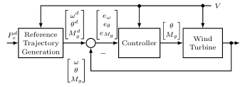
Figure 4: Closed-loop structure of the new control scheme.

4.1 Augmented State Model

In Figure 5, a detailed overview of the controller block in Figure 4 is shown. For accurate tracking of the reference generator speed $\omega^{d}$, the integral $z(k)$ of the error

$$e_{\omega}(k)=\omega^{d}(k)-\omega(k)=\xi^{d}(k)-\xi(k),$$ (29)

is added to the model (see, e.g., Birla and Swarup, 2015).

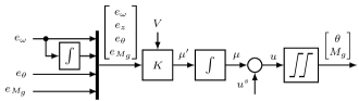
Figure 5: Internal structure of the new controller.

Moreover, the inputs $\mu(k)=\begin{bmatrix}\mu_{1}(k)&\mu_{2}(k)\end{bmatrix}^{T}\in\mathbb{R}^{2}$ are moved into the state vector and new differential inputs $\mu^{\prime}(k)\in\mathbb{R}^{2}$ are added to the model. This allows to discourage actuation changes that cause mechanical wear in the LQ optimal control design. Together with (29), this results in the augmented system

$$\begin{bmatrix}\xi(k+1)\\ z(k+1)\\ \mu(k+1)\end{bmatrix}=\begin{bmatrix}A_{\text{d}}\xi(k)+B_{\text{d}}\mu(k)+F_{\text{d}}\nu(k)\\ z(k)+T_{s}\xi^{d}(k)-T_{s}\xi(k)\\ \mu(k)+T_{s}\mu^{\prime}(k)\end{bmatrix}.$$ (30)

This can be reformulated into

$$x(k+1)=Ax(k)+B\mu^{\prime}(k)+F\tilde{\nu}(k),$$ (31)

with state $x(k)=\begin{bmatrix}\xi(k)&z(k)&\mu(k)^{T}\end{bmatrix}^{T}$, external inputs $\tilde{\nu}(k)=\begin{bmatrix}\nu(k)&\xi^{d}(k)\end{bmatrix}^{T}$, and matrices

$$A=\begin{bmatrix}A_{\text{d}}&0&B_{\text{d}}\\ -T_{s}&1&0^{T}_{2}\\ 0_{2}&0_{2}&I_{2}\end{bmatrix},\quad B=\begin{bmatrix}0^{T}_{2}\\ 0^{T}_{2}\\ T_{s}I_{2}\end{bmatrix},\quad F=\begin{bmatrix}F_{d}&0\\ 0&T_{s}\\ 0_{2}&0_{2}\end{bmatrix}.$$

Note that, the desired generator speed deviation $\xi^{d}(k)$ is included as an external input, which is provided through the reference trajectory generation block.

4.2 LQ Optimal Control

The LQ optimal controller is designed for the augmented state model (31), which is controllable. The controller uses linear state feedback of the form ${u(k)=-Kx(k)}$, with gain matrix $K\in\mathbb{R}^{p\times n}$, to drive the system to the origin. To drive the system close to a desired state $x^{d}(k)\in\mathbb{R}^{n}$, the control law is modified, into ${u(k)=K(x^{d}(k)-x(k))}$ (Skogestad and Postlethwaite, 2005). Matrix $K$ is computed such that the cost function

$$J=\sum_{n=1}^{\infty}x(k)^{T}Q\,x(k)+u(k)^{T}R\,u(k),$$ (32)

with positive semidefinite $Q\in\mathbb{R}^{4\times 4}$ and positive definite $R\in\mathbb{R}^{2\times 2}$ is minimized. The values used for $Q$ and $R$ can be found in Tab. 3. We can find a solution via the discrete-time Riccati equation

$$A^{T}S\,A-S-A^{T}S\,B(B^{T}S\,B+R)^{-1}B^{T}S\,A+Q=0.$$ (33)

Solving (33) provides $S\in\mathbb{R}^{4\times 4}$ from which we obtain

$$K=(B^{T}S\,B+R)^{-1}B^{T}S\,A.$$ (34)

4.3 Switching Controller

Due to distinct operating regions (see Figure 2), two gain matrices $K_{1}$ and $K_{2}$ are computed based on the linearized model for two different equilibrium points. Additionally, the cost function is different for both gain matrices, in particular, for $K_{1}$, the generator speed must be tracked very accurately to maximize power production. For $K_{2}$, the cost function is adjusted such that the generator speed and torque are tracked accurately to satisfy the power demand, this is reflected in the weight matrices in Tab. 3. The gain matrix $K(k)\in\mathbb{R}^{2\times 4}$ is then determined by switching between $K_{1}$ and $K_{2}$ based on a hysteresis. Once the wind speed rises above the upper wind speed threshold $\overline{V}\in\mathbb{R}^{+}$, $K_{2}$ is selected as the active gain matrix. As soon as the wind speed drops below a lower wind speed threshold $\underline{V}\in\mathbb{R}^{+}$ with $\underline{V}<\overline{V}$, $K_{1}$ is selected, i.e.,

$$K(k)=\begin{cases}K_{1}\quad&\text{if }V(k)<\underline{V},\\ K(k-1)&\text{if }\underline{V}\leq V(k)\leq\overline{V},\\ K_{2}&\text{if }\overline{V}<V(k).\end{cases}$$ (35)

This completes the controller implementation. Before the controller can be used, reference trajectories need be generated.

4.4 Reference Trajectories

The desired state

$$x^{d}(k)=\begin{bmatrix}\omega^{d}(k)&z^{d}(k)&\theta^{d}(k)&M_{g}^{d}(k)\end{bmatrix}^{T}-\begin{bmatrix}\omega^{s}&0&\theta^{s}&M_{g}^{s}\end{bmatrix}^{T},$$

contains the reference generator speed $\omega^{d}(k)$, the reference integral error $z^{d}(k)$, the reference pitch angle $\theta^{d}(k)$, the reference generator torque $M_{g}^{d}(k)$, and the equilibrium $(\omega^{s},\begin{bmatrix}\theta^{s}&M_{g}^{s}\end{bmatrix}^{T})$. Clearly, no integral error is desired, i.e. $z^{d}(k)=0$. The derivation of the remaining references will be discussed in what follows.

4.4.1 Reference Generator Speed:

The reference generator speed is the minimum of $\omega^{*}(k)$ and the power setpoint speed $\omega^{sp}(k)$, i.e.,

$$\hat{\omega}^{d}(k)=\min\big{(}\omega^{*}(k),\,\omega^{sp}(k)\big{)}.$$ (36)

Here, $\omega^{*}(k)$ is found by maximizing the power coefficient (8) for the current pitch angle $\theta(k)$ and wind speed $V(k)$. Thus, the problem

$$\max_{\omega(k)} \quad\hat{C}_{p}\bigg{(}\frac{r}{N_{g}}\frac{\omega(k)}{V(k)},\theta(k)\bigg{)},$$ (37a)

s.t. $$\quad\Big{(}\frac{r}{N_{g}}\frac{\omega(k)}{V(k)},\theta(k)\Big{)}\in\mathbb{H},$$ (37b)

is solved to obtain $\omega^{*}(k)$. The power setpoint speed $\omega^{sp}(k)$ is computed using a lookup table depending on $P^{d}_{e}(k)$, i.e.,

$$\omega^{sp}(k)=\operatorname{LUT}\big{(}P^{d}_{e}(k)\big{)}.$$ (38)

Analogously to Kim et al. (2018) and Jeon et al. (2021), steady state simulation data is used to deduce the lookup table. Here, steady state equilibria tuples of generator speed and output power are aranged in a grid. This provides an adaptable basis and realizes a simple to use while effective method to convert the desired power into a reference trajectory for the generator speed.

For the reference generator speed $\omega^{d}(k)$, a lowpass filter is applied to $\hat{\omega}^{d}(k)$, i.e.,

$$\omega^{d}(k)=(1-\alpha_{1})\cdot\omega^{d}(k-1)+\alpha_{1}\cdot\hat{\omega}^{d}(k),$$ (39)

where $\alpha_{1}=\frac{T_{s}}{T_{1}+T_{s}}\in[0,1]\subset\mathbb{R}^{+}_{0}$ is based on $T_{s}$ and the filter time constant $T_{1}$, with $\omega^{d}(0)=\hat{\omega}^{d}(k)$.

4.4.2 Reference Pitch:

The reference pitch angle

$$\hat{\theta}^{d}(k)=\operatorname{LUT}\big{(}P^{d}_{e}(k),V(k)\big{)},$$ (40)

is computed with a lookup table from the same steady state simulation data as in (38). To prevent fast changes $\hat{\theta}^{d}(k)$ is lowpass filtered via

$$\theta^{d}(k)=(1-\alpha_{2})\cdot\theta^{d}(k)+\alpha_{2}\cdot\hat{\theta}^{d}(k).$$ (41)

Here, $\alpha_{2}=\frac{T_{s}}{T_{2}+T_{s}}\in[0,1]$, is based on $T_{s}$ and the filter time constant $T_{2}$, with $\theta^{d}(0)=\hat{\theta}^{d}(0)$.

4.4.3 Reference Generator Torque:

The reference generator torque is computed such that once $\omega^{d}(k)$ is reached, exactly the demanded power is produced. Assuming a perfect generator speed tracking, solving (10) for $M_{g}(k)$ results in

$$M_{g}^{d}(k)=\frac{P_{e}^{d}(k)}{\eta\omega^{d}(k)}.$$ (42)

4.5 Control Law

Finally, the plant is controlled with the input $u(k)$ which is derived by integrating $\mu^{\prime}$, i.e.,

$$u(k)=\mu(k)+u^{s}(k)=\mu(k-1)+T_{s}\cdot\mu^{\prime}(k)+u^{s}(k),$$ (43)

where $u^{s}(k)$ denotes the steady state inputs $\begin{bmatrix}\theta^{s}&M_{g}^{s}\end{bmatrix}^{T}$ of the currently active controller. The differential input $\mu^{\prime}(k)$ is computed by the gain matrix $K(k)$ and the error from the reference $x^{d}(k)$, i.e.,

$$\mu^{\prime}(k)=K(k)\cdot\big{(}x^{d}(k)-x(k)\big{)}.$$ (44)

Combined into one, the control input $u(k)$ is obtained from

$$u(k)=\mu(k-1)+T_{s}\cdot K(k)\cdot\big{(}x^{d}(k)-x(k)\big{)}+u^{s}(k).$$ (45)

Before applying the inputs to the plant, saturation and slew rate constraints are enforced

$$\theta(k) =\theta(k-1)+\mathop{\ThisStyle{\raisebox{-2.4pt}{\kern 0.5pt\LMpt\scaleto{ \leavevmode\hbox to428.34pt{\vbox to428.34pt{\text{[drawing]}}}}{2.25\LMex}\kern 0.5pt\LMpt}}}_{\underline{\Delta\theta}}^{\overline{\Delta\theta}}\bigg{(}\mathop{\ThisStyle{\raisebox{-2.4pt}{\kern 0.5pt\LMpt\scaleto{ \leavevmode\hbox to428.34pt{\vbox to428.34pt{\text{[drawing]}}}}{2.25\LMex}\kern 0.5pt\LMpt}}}_{\underline{\theta}}^{\overline{\theta}}\big{(}\theta^{t}(k)\big{)}-\theta(k-1)\bigg{)},$$ (46)

$$M_{g}(k) =M_{g}(k-1)+$$ (47)

$$\quad\quad\quad\quad\mathop{\ThisStyle{\raisebox{-2.4pt}{\kern 0.5pt\LMpt\scaleto{ \leavevmode\hbox to428.34pt{\vbox to428.34pt{\text{[drawing]}}}}{2.25\LMex}\kern 0.5pt\LMpt}}}_{\underline{\Delta M}_{g}}^{\overline{\Delta M}_{g}}\bigg{(}\mathop{\ThisStyle{\raisebox{-2.4pt}{\kern 0.5pt\LMpt\scaleto{ \leavevmode\hbox to428.34pt{\vbox to428.34pt{\text{[drawing]}}}}{2.25\LMex}\kern 0.5pt\LMpt}}}_{\underline{M}_{g}}^{\overline{M}_{g}}\big{(}M_{g}^{t}(k)\big{)}-M_{g}(k-1)\bigg{)}.$$ (48)

5 Case Study

In this section, the LQ optimal controller, from Section 4, is compared with the baseline controller, from Section 3. The IEA $3.35\text{\,}\mathrm{MW}$ wind turbine (Bortolotti et al., 2019) is used for all simulations. The corresponding turbine parameters, such as bounds on the control inputs, their rates of change, and others are presented in Table 1. In Table 2, the baseline controller parameter values from Bortolotti et al. (2019) are listed. In Table 3, the LQ optimal controller parameters are listed, and in Table 4, the parameters for (8) are provided. These were determined based on the data points provided by Bortolotti et al. (2019).

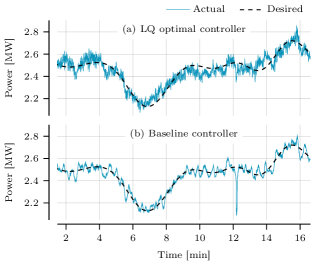
Figure 6: Output power trajectories.

All simulations are executed with a sampling time of ${T_{s}=$4\text{\,}\mathrm{ms}$}$. From each simulation, the first $1.5\text{\,}\mathrm{min}$ are omitted to disregard transient simulation effects.

Power tracking in Region III is evaluated with an average wind speed of $15\text{\,}\frac{\mathrm{m}}{\mathrm{s}}$ and a turbulence intensity of $9\text{\,}\mathrm{\char 37\relax}$. In Figure 6, the output power of both controllers, as well as the desired power are shown. The LQ optimal controller and the baseline controller both achieve similar root-mean-square (RMS) tracking errors of $45.1\text{\,}\mathrm{kW}$ and $44.1\text{\,}\mathrm{kW}$, respectively. This represents a relative error below $2\text{\,}\mathrm{\char 37\relax}$ of the rated power. A notable difference between the two controllers appears around $t=$12.2\text{\,}\mathrm{min}$$, where the baseline controller dips far below the desired power. In contrast, the LQ optimal controller remains much closer to the desired value.

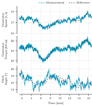
Figure 7: Reference tracking plots at $15\text{\,}\mathrm{m}\text{/}\mathrm{s}$ wind speed with $9\text{\,}\mathrm{\char 37\relax}$ turbulence intensity.

Figure 7 presents the measurements and reference signals for generator speed, generator torque, and pitch angle for the LQ optimal controller from the same simulation as in Figure 6. The three reference trajectories are tracked with different accuracies. The generator speed and pitch angle references are only tracked approximately. In contrast, the generator torque signal tracks the reference very well due to its relatively high weight in $Q_{2}$ (see Table 3).

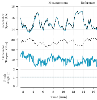
Figure 8: Reference tracking plots at $6.3\text{\,}\mathrm{m}\text{/}\mathrm{s}$ wind speed with $9\text{\,}\mathrm{\char 37\relax}$ turbulence intensity.

Typically in Region II, the wind speed does not allow for power tracking of arbitrary power demands. In Figure 8, measurements and reference signals for generator speed, generator torque, and pitch angle are shown for a wind speed of $6.3\text{\,}\frac{\mathrm{m}}{\mathrm{s}}$ with a turbulence intensity of $9\text{\,}\mathrm{\char 37\relax}$.

The tracking behavior differs vastly from the results in Figure 7. The generator speed and pitch angle are tracked very closely but the generator torque deviates from its reference. In detail, pitch angle reference and measurement remain at the optimal value of $1.09\text{\,}\mathrm{\SIUnitSymbolDegree}$, which originates from the blade geometry. Tracking the reference generator speed closely is important to remain at the optimal tip-speed ratio. In combination with the optimal pitch angle, this allows to extract maximum power from the wind. Due to low wind speeds, which are not sufficient to achieve the desired output power, the torque of the generator cannot be tracked accurately without decelerating the turbine as thereby deviating from the generator speed reference. To stop the turbine from slowing down, deviations are acceptable and desired, hence the low weight in the fourth entry in $Q_{1}$ (see Table 3).

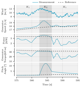
Figure 9: Measurements while switching.

In Figure 9, the wind speed, generator speed, output power, generator torque, and pitch angle are shown during the switching along with their reference trajectories. The light gray area marks the use of $K_{1}$, the darker area the use of $K_{2}$. At the border between both areas, the controller switches and therefore nonsmooth trajectories may occur. Beginning at $t=$579\text{\,}\mathrm{s}$$, the wind speed starts to increase. Then, at $t=$581\text{\,}\mathrm{s}$$, the generator torque reaches its maximum. From that point on the generator speed starts to increase. At $t=$582.5\text{\,}\mathrm{s}$$, $\overline{V}=$12\text{\,}\frac{\mathrm{m}}{\mathrm{s}}$$ is reached, the controller switches and immediately the pitch angle is increased to decelerate the wind turbine. After a few seconds, the wind speed drops below $\underline{V}=$10\text{\,}\frac{\mathrm{m}}{\mathrm{s}}$$, the controller switches back to $K_{1}$, and the pitch angle slowly returns to its reference value. During the switching, no jumps occured and all trajectories were reasonably smooth.

Another important aspect, when designing wind turbine controllers are mechanical loads that lead to wear. In Figure 10, some important damage equivalent loads are displayed for different scenarios.

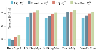
Figure 10: Damage equivalent loads for both controllers and two different power demand signals. The blade root out-of-plane bending moment (RootMyc1), the shaft non-rotating out-of-plane bending moment (LSSGagMys), the shaft non-rotating yaw bending moment (LSSGagMzs), the tower top fore-aft bending moment (YawBrMyn), and the tower top torsion bending moment (YawBrMzn).

The rainflow counting algorithm (Dowling, 1971) is employed to compute the damage amplitudes (Burton et al., 2011). The DELs are computed for 5 different turbine components in Figure 10, which are prone to mechanical wear. The baseline controller is compared with the LQ optimal controller for two different power demand scenarios. First, a variable power demand $P^{d}_{e}$ is tracked, in the second scenario the power demand is set to the nominal $P^{N}=$3.35\text{\,}\mathrm{MW}$$. In both scenarios, a wind with an average of $15\text{\,}\frac{\mathrm{m}}{\mathrm{s}}$ and a turbulence intensity of $9\text{\,}\mathrm{\char 37\relax}$ is considered. For all components except the blade root out-of-plane bending moment (RootMyc1), the LQ optimal controller achieves lower DELs for both power demand scenarios and therefore causes less mechanical wear. The blade root out-of-plane bending moment poses an exception, where during the power tracking the LQ optimal controller leads to slightly higher DEL than the baseline controller. However, overall an average load reduction of $2.3\text{\,}\mathrm{\char 37\relax}$ could be achieved with the LQ optimal controller, while achieving comparable performance in power tracking.

6 Conclusion

We showed that a multivariable LQ optimal control approach in combination with a relatively simple reference trajectory generation scheme achieves state-of-the-art performance with regard to power tracking. The presented results indicate that considering the input coupling (in the LQ optimal control design) is more important than considering nonlinearities (as done by the state-of-the-art controller). The modular control scheme allows to further improve reference trajectories which can lead to even better performance. We also showed that the LQ optimal controller achieves lower DELs throughout most simulations in comparison with the state-of-the-art.

In future work, multiple improvements are planned to be explored. Such as relaxing the assumption that accurate wind speed measurements are available. Moreover, the computation of the reference trajectories shall be expanded to enable better performance of the LQ optimal controller. Finally, alternative linear multivariable control schemes will be considered.

Appendix A Simulation Parameters

Table 1: IEA $3.35\text{\,}\mathrm{MW}$ turbine parameters.

$J_{t}=$39\,825\,631\text{\,}\mathrm{kg}\text{\,}{\mathrm{m}}^{2}$$, $r=$65\text{\,}\mathrm{m}$$, $\rho=$1.225\text{\,}\frac{\mathrm{kg}}{{\mathrm{m}}^{3}}$$, $\eta=$93.6\text{\,}\mathrm{\char 37\relax}$$,

$N_{g}=$97\text{\,}$$, $\omega_{g}^{\text{Rated}}=$1.35\text{\,}\frac{\mathrm{rad}}{\mathrm{s}}$$, $M_{g}^{\text{Rated}}=$30.15\text{\,}\mathrm{kN}\text{\,}\mathrm{m}$$, $\underline{\theta}=$1.09\text{\,}\mathrm{\SIUnitSymbolDegree}$$,

$\overline{\theta}=$22\text{\,}\mathrm{\SIUnitSymbolDegree}$$, $\underline{\Delta\theta}=$-0.000\,488\text{\,}\frac{\mathrm{\SIUnitSymbolDegree}}{}$$, $\overline{\Delta\theta}=$0.000\,488\text{\,}\frac{\mathrm{\SIUnitSymbolDegree}}{}$$,

$\overline{M}_{g}=$33.17\text{\,}\mathrm{kN}\text{\,}\mathrm{m}$$, $\underline{M}_{g}=$0\text{\,}$$, $\underline{\Delta M}_{g}=$-6\text{\,}\frac{\mathrm{kN}\text{\,}\mathrm{m}}{}$$, $\overline{\Delta M}_{g}=$6\text{\,}\frac{\mathrm{kN}\text{\,}\mathrm{m}}{}$$,

Table 2: Baseline controller parameter configuration.

$c_{12}=$82.47\text{\,}\mathrm{N}\text{\,}\mathrm{m}\text{\,}\mathrm{s}$$, $\omega_{\text{ci}}=$10.47\text{\,}\frac{\mathrm{rad}}{\mathrm{s}}$$, $c_{M}^{*}=$1.75\text{\,}\mathrm{N}\text{\,}\mathrm{m}\text{\,}{\mathrm{s}}^{2}$$,

$\omega_{\text{r2}}=$15.71\text{\,}\frac{\mathrm{rad}}{\mathrm{s}}$$, $T_{M}=$1\text{\,}\mathrm{s}$$, $c_{\theta}^{\text{GB}}=$30\text{\,}\frac{\mathrm{rad}}{\mathrm{s}\text{\,}\mathrm{\SIUnitSymbolDegree}}$$,

$T_{\theta}=$0.133\text{\,}\mathrm{s}$$, $T_{\text{GB}}=$10\text{\,}\mathrm{s}$$, $c_{M}^{\text{GB}}=$0.0001\text{\,}\frac{\mathrm{rad}}{\mathrm{s}\text{\,}\mathrm{N}\text{\,}\mathrm{m}}$$,

$K_{K}=$0.174\text{\,}\mathrm{\SIUnitSymbolDegree}$$, $K_{I}=$0.004\text{\,}\mathrm{\SIUnitSymbolDegree}\text{\,}\mathrm{s}$$, $K_{P}=$0.133\text{\,}\mathrm{\SIUnitSymbolDegree}\text{\,}\mathrm{s}$$,

Table 3: LQ optimal controller configuration parameters.

$\omega_{1}^{s}=$119.31\text{\,}\frac{\mathrm{rad}}{\mathrm{s}}$$, $\theta_{1}^{s}=$2.65\text{\,}\mathrm{\SIUnitSymbolDegree}$$, $M_{g,1}^{s}=$16.85\text{\,}\mathrm{kN}\text{\,}\mathrm{m}$$,

$V_{1}^{s}=$8\text{\,}\frac{\mathrm{m}}{\mathrm{s}}$$, $V_{2}^{s}=$10.5\text{\,}\frac{\mathrm{m}}{\mathrm{s}}$$,

$Q_{1}=\operatorname{diag}(10^{-2},10^{3},10^{3},10^{-2})$, $R_{1}=\operatorname{diag}(5\cdot 10^{4},5\cdot 10^{4})$,

$\omega_{2}^{s}=$119.31\text{\,}\frac{\mathrm{rad}}{\mathrm{s}}$$, $\theta_{2}^{s}=$6.98\text{\,}\mathrm{\SIUnitSymbolDegree}$$, $M_{g,2}^{s}=$25.72\text{\,}\mathrm{kN}\text{\,}\mathrm{m}$$,

$Q_{2}=\operatorname{diag}(10^{-4},10,10^{4},10^{6})$, $R_{2}=\operatorname{diag}(10^{6},10^{4})$,

$T_{1}=$20\text{\,}\mathrm{s}$$, $T_{2}=$40\text{\,}\mathrm{s}$$, $\underline{V}=$10\text{\,}\frac{\mathrm{m}}{\mathrm{s}}$$, $\overline{V}=$12\text{\,}\frac{\mathrm{m}}{\mathrm{s}}$$,

Table 4: Power coefficient parameters computed by fitting the function to steady-state simulation data.

$c_{1}=$0.098\text{\,}$$, $c_{2}=$-0.150\text{\,}$$, $c_{3}=$-0.011\text{\,}\frac{}{\mathrm{\SIUnitSymbolDegree}}$$,

$c_{4}=$0.061\text{\,}$$, $c_{5}=$0.0125\text{\,}\frac{}{\mathrm{\SIUnitSymbolDegree}}$$, $c_{6}=$0.000\,053\text{\,}\frac{}{\mathrm{{}^{\circ^{2}}}}$$,

$c_{7}=$-0.006\,15\text{\,}$$, $c_{8}=$-0.001\,84\text{\,}\frac{}{\mathrm{\SIUnitSymbolDegree}}$$,

$c_{9}=$-0.000\,338\text{\,}\frac{}{\mathrm{{}^{\circ^{2}}}}$$, $c_{10}=$0.000\,040\,7\text{\,}\frac{}{\mathrm{{}^{\circ^{3}}}}$$,

$c_{11}=$0.000\,184\text{\,}$$, $c_{12}=$0.000\,106\text{\,}\frac{}{\mathrm{\SIUnitSymbolDegree}}$$,

$c_{13}=$-0.000\,051\,5\text{\,}\frac{}{\mathrm{{}^{\circ^{2}}}}$$, $c_{14}=$0.000\,014\,3\text{\,}\frac{}{\mathrm{{}^{\circ^{3}}}}$$,

$c_{15}=$-0.000\,001\,97\text{\,}\frac{}{\mathrm{{}^{\circ^{4}}}}$$,

References

- Aho et al. (2012) Aho, J., Buckspan, A., Laks, J., Fleming, P., Jeong, Y., Dunne, F., Churchfield, M., Pao, L., and Johnson, K. (2012). Tutorial of Wind Turbine Control for Supporting Grid Frequency through Active Power Control. In Am. Control Conf., 3120–3131.
- Aho et al. (2013) Aho, J., Pao, L., and Fleming, P. (2013). An Active Power Control System for Wind Turbines Capable of Primary and Secondary Frequency Control for Supporting Grid Reliability. In Proc. 2012 AIAA/ASME Wind Symp.
- Birla and Swarup (2015) Birla, N. and Swarup, A. (2015). Optimal preview control: A review. Optim. Control Appl. Methods, 241–268.
- Boersma et al. (2017) Boersma, S., Doekemeijer, B., Gebraad, P., Fleming, P., Annoni, J., Scholbrock, A., Frederik, J.A., and van Wingerden, J.W. (2017). A Tutorial on Control-Oriented Modeling and Control of Wind Farms. In Am. Control Conf., 1–18.
- Bortolotti et al. (2019) Bortolotti, P., Tarres, H.C., Dykes, K., Merz, K., Sethuraman, L., Verelst, D., and Zahle, F. (2019). IEA Wind Task 37 on Systems Engineering in Wind Energy – WP2.1 Reference Wind Turbines. Technical report, Int. Energy Agency. URL https://www.nrel.gov/docs/fy19osti/73492.pdf.
- Burton et al. (2011) Burton, T., Jenkins, N., Sharpe, D., and Bossanyi, E. (2011). Wind Energy Handbook. John Wiley & Sons.
- Child et al. (2019) Child, M., Kemfert, C., Bogdanov, D., and Breyer, C. (2019). Flexible electricity generation, grid exchange and storage for the transition to a 100% renewable energy system in Europe. Renew. Energ., 139, 80–101.
- Dowling (1971) Dowling, N.E. (1971). Fatigue Failure Predictions for Complicated Stress Strain Histories. Technical report, University of Illinois at Urbana-Champaign.
- Hansen (2008) Hansen, M.O.L. (2008). Aerodynamics of Wind Turbines. Earthscan, Sterling, VA.
- Jeon et al. (2021) Jeon, T., Kim, D., Song, Y., and Paek, I. (2021). Design and Validation of Demanded Power Point Tracking Control Algorithm for MIMO Controllers in Wind Turbines. Energies, 14(18), 5818.
- Jonkman et al. (2022) Jonkman, B., Mudafort, R.M., Platt, A., Branlard, E., and Sprague, M. (2022). Openfast/openfast: Openfast v3.1.0. 10.5281/zenodo.6324288. URL https://doi.org/10.5281/zenodo.6324288.
- Jonkman et al. (2009) Jonkman, J., Butterfield, S., Musial, W., and Scott, G. (2009). Definition of a 5-MW Reference Wind Turbine for Offshore System Development. Technical report, NREL, Golden, CO (United States).
- Kelley et al. (2007) Kelley, N.D., Jonkman, B.J., Scott, G.N., and Pichugina, Y.L. (2007). Comparing Pulsed doppler LIDAR with SODAR and Direct Measurements for Wind Assessment. Technical report, NREL, Golden, CO (United States).
- Kim et al. (2018) Kim, K., Kim, H.G., Kim, C.j., Paek, I., Bottasso, C.L., and Campagnolo, F. (2018). Design and Validation of Demanded Power Point Tracking Control Algorithm of Wind Turbine. Int. J. Precis. Eng. Manuf.-Green Technol., 5(3), 387–400.
- Luz et al. (2018) Luz, T., Moura, P., and de Almeida, A. (2018). Multi-objective power generation expansion planning with high penetration of renewables. Renew. Sustain. Energy Rev., 81, 2637–2643.
- Merabet et al. (2011) Merabet, A., Thongam, J., and Gu, J. (2011). Torque and Pitch Angle Control for Variable Speed Wind Turbines in All Operating Regimes. In Int. Conf. Environ. Electr. Eng., 1–5. IEEE.
- Mirzaei et al. (2013) Mirzaei, M., Soltani, M., Poulsen, N.K., and Niemann, H.H. (2013). An MPC approach to individual pitch control of wind turbines using uncertain LIDAR measurements. In Eur. Control Conf., 490–495.
- Ostergaard et al. (2007) Ostergaard, K.Z., Brath, P., and Stoustrup, J. (2007). Gain-Scheduled Linear Quadratic Control of Wind Turbines Operating at High Wind Speed. In Int. Conf. Control Appl., 276–281. IEEE.
- Pullen and Sawyer (2011) Pullen, A. and Sawyer, S. (2011). Global Wind Report: Annual market update 2010. World Wind Energy Conf.
- Schlipf (2016) Schlipf, D. (2016). Lidar-Assisted Control Concepts for Wind Turbines. Verlag Dr. Hut.
- Skogestad and Postlethwaite (2005) Skogestad, S. and Postlethwaite, I. (2005). Multivariable Feedback Control: Analysis and Design. John Wiley & Sons.
- Wagner (2020) Wagner, H.J. (2020). Introduction to wind energy systems. In EPJ Web Conf., volume 246, 00004. EDP Sciences.