Constraining axion and compact dark matter with interstellar medium heating

Abstract

Cold interstellar gas systems have been used to constrain dark matter (DM) models by the condition that the heating rate from DM must be lower than the astrophysical cooling rate of the gas. Following the methodology of Wadekar and Farrar (2021), we use the interstellar medium of a gas-rich dwarf galaxy, Leo T, and a Milky Way-environment gas cloud, G33.4-8.0 to constrain DM. Leo T is a particularly strong system as its gas can have the lowest cooling rate among all the objects in the late Universe (owing to the low volume density and metallicity of the gas). Milky Way clouds, in some cases, provide complementary limits as the DM-gas relative velocity in them is much larger than that in Leo T. We derive constraints on the following scenarios in which DM can heat the gas: $(i)$ interaction of axions with hydrogen atoms or free electrons in the gas, $(ii)$ deceleration of relic magnetically charged DM in gas plasma, $(iii)$ dynamical friction from compact DM, $(iv)$ hard sphere scattering of composite DM with gas. Our limits are complementary to DM direct detection searches. Detection of more gas-rich low-mass dwarfs like Leo T from upcoming 21cm and optical surveys can improve our bounds.

I Introduction

There are a number of well-motivated models of dark matter (DM) that feature couplings to Standard Model (SM) particles or self interactions. A popular example is the QCD axion Peccei and Quinn (1977); Weinberg (1978); Wilczek (1978), which is natural to have couplings to photons, leptons and nucleons. Such interactions can be potentially detected in laboratory and astrophysical measurements, but are still consistent with cold DM (CDM) at large scale. DM can also be made up of compact objects; these can have macroscopic interactions with ordinary matter. There can also be candidates such as primordial black holes (PBHs) Green and Kavanagh (2021) which emit SM particles by Hawking radiation and can accrete matter around them. Constraining the interactions of DM is critical to both DM model building and instrumental development.

Direct and indirect detection are two particularly important techniques to discover DM interactions. The strategy of direct detection is to look for signals of nucleon (electron) recoil caused by DM-nucleon (-electron) scattering using Earth-based laboratory detectors such as XENON Aprile et al. (2020). Limits on DM interactions from these experiments, despite being exceedingly stringent, suffer from the overburden effect Zaharijas and Farrar (2005), and do not apply to sufficiently large cross sections. Due to trigger sensitivity, most of the experiments must require DM particles to be heavy enough, typically $>\order{1}$ GeV for DM-nucleon scattering. In addition to laboratory detectors, a variety of astrophysical systems have also been used to probe DM scattering with SM particles and provide complementary limits, such as CMB Xu et al. (2018), the population of satellite galaxies Nadler et al. (2019), planets Farrar and Zaharijas (2006) and exoplanets Leane and Smirnov (2021). These astrophysical limits are generally weaker than laboratory limits, but have the advantage of evading the overburden effect and also can be applied to much lighter DM particles. In contrast to directly searches, indirect searches look for visible products of DM decay or annihilation. Limits on decay lifetime and annihilation cross section have been derived from X/$\gamma$-ray telescopes Essig et al. (2013); Abdallah et al. (2018), CMB anisotropy Slatyer and Wu (2017), CMB spectal distortion Bolliet et al. (2020); Ali-Haïmoud (2021), line-intensity mapping Bernal et al. (2021), dwarf spheroid galaxies Albert et al. (2017) (see however Ando et al. (2020)), Lyman-$\alpha$ forests Liu et al. (2021) and cosmic rays Accardo et al. (2014).

Recently, it shown that some of the gas-rich astrophysical systems can be used as powerful calorimetric DM detectors Chivukula et al. (1990); Dubovsky and Hernández-Chifflet (2015); Wadekar and Farrar (2021); Bhoonah et al. (2018, 2018, 2021); Farrar et al. (2020). These studies required that DM heat injection rate $\dot{Q}_{\mathrm{DM}}$ must be lower than the astrophysical cooling rate of the gas $\dot{C}$,

$$\dot{Q}_{\mathrm{DM}}\leq\dot{C}\,,$$ (1)

otherwise the temperature of the gas would steadily increase (and the ionization state of the gas could also be altered). Systems with low gas cooling rates are therefore more sensitive to energy injections by DM. To our best knowledge, warm neutral gas in the Leo T dwarf galaxy has the lowest cooling rate among astrophysical systems in the late Universe (see the comparison in Fig. 1). This is precisely why Ref. Wadekar and Farrar (2021) used Leo T to constrain heating due to DM.

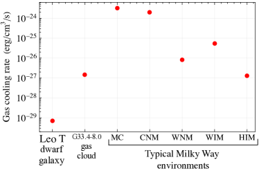
Figure 1: Estimates of astrophysical radiative cooling rate of the gas in Leo T, G33.4$-$8.0 cloud, and typical Milky Way interstellar medium phases. Cooling rates generally decrease with lower gas density, metal fraction and temperatures (see section II for further details). Due to its low metallicity and gas volume density, the gas in Leo T has a much lower astrophysical cooling rate than typical systems in the Milky Way (to our best knowledge, gas in Leo T has the lowest cooling rate among astrophysical systems in the late Universe).

In particular, Ref. Wadekar and Farrar (2021) derived limits on DM-nucleon/electron scattering cross sections, and the mixing parameter of dark photon DM. Refs. Lu et al. (2021); Laha et al. (2020); Kim (2021); Takhistov et al. (2021a, b) used Leo T to constrain various heating mechanisms due to primordial black holes (PBH) (e.g., Hawking radiation, accretion disk, outflows and dynamical friction), and obtained upper bounds on the abundance of PBHs. In an earlier work Wadekar and Wang (2022), we used Leo T to place limits on DM decay and annihilation to $e^{+}e^{-}$ and $\gamma\gamma$ pairs, updating existing limits for $\order{100\,\mathrm{eV}}$ photons and $\order{1\,\mathrm{MeV}}$ electrons.

To set strong bounds on DM, not only should $\dot{C}$ in Eq. 1 be lower, but $\dot{Q}_{\mathrm{DM}}$ also should be larger. There are many models of DM where $\dot{Q}_{\mathrm{DM}}$ increases as a function of DM-gas relative velocity (e.g., in the scenario where cross section of DM-baryon interactions is velocity-independent, $\dot{Q}_{\mathrm{DM}}\propto v^{3}_{\mathrm{relative}}$). Leo T has low relative velocity between DM and baryons $\sim 17$ km/s, whereas systems in the Milky Way (MW) have $v_{\mathrm{relative}}\sim 300$ km/s. Therefore, in such scenarios, MW systems can potentially provide stronger limits than Leo T. A variety of MW gas clouds have therefore been used for constraining DM models such as millicharged DM, asymmetric DM nuggets, DM-nuclei contact interactions, magnetically charged black holes and DM decay/annihilation Bhoonah et al. (2018, 2021); Diamond and Kaplan (2022); Wadekar and Wang (2022)

In this paper, we will use both the Leo T galaxy and a robust MW gas cloud, G33.4-8.0 Farrar et al. (2020), to constrain DM heating (hereafter, we use the phrase, the MW cloud, to refer to G33.4-8.0). We derive new limits on a few DM models using the interstellar gas heating argument, as well as update certain existing limits that used inaccurate inputs. The paper is organized as follows. In Sec. II, we review the properties of the gas systems. In Sec. III, we study the heating due to electrophilic axion DM and set limits on the electron coupling. In Sec. IV, we derive limits on heat injection from compact DM objects via dynamical friction, hard sphere scattering and magnetic effects.

II Properties of Leo T and Milky Way gas cloud

In this section, we discuss properties of the astrophysical systems and the formalism for calculating their radiative gas cooling rate $\dot{C}$. Depending on the temperature and ionization fraction of the gas, interstellar gas systems can be generically classified to five types: molecular clouds (MC), cold neutral medium (CNM), warm neutral medium (WNM), warm ionized medium (WIM), and hot ionized medium (HIM) Draine (2011). The gas in the inner part of the Leo T galaxy is dominated by WNM with $T\simeq 6100$ K Ryan-Weber et al. (2008); Adams and Oosterloo (2018). The spatial profile of DM, hydrogen, and free electrons in Leo T was determined by Ref. Faerman et al. (2013) upon fitting a hydrostatic model to Hi  column density observations and assuming that the DM follows a Burkert (cored) profile Burkert (1995):

$$\rho_{\mathrm{DM}}=\frac{\rho_{0}}{(1+\frac{r}{r_{s}})(1+\frac{r^{2}}{r^{2}_{s}})}$$ (2)

where $r$ is the radial distance from the halo center, $r_{s}$ is the scale radius and $\rho_{0}$ is the central core density. Recent observations suggest the presence of roughly constant density cores in most of the low-mass dwarf galaxies, therefore the choice of Burkert profile for Leo T is well-motivated. Furthermore, assuming a cuspy profile (e.g., NFW) will give tighter constraints on DM, hence our assumption of cored profiles is conservative. The best-fit profiles from Ref. Faerman et al. (2013) are shown in Fig. 6 (corresponding to $\rho_{0}=3.9$ GeV/cm³ and $r_{s}=0.7$ kpc for the DM halo), and we adopt them for our calculations.

A widely-used approximate formula to calculate the cooling rate is Smith et al. (2017)

$$\dot{C}=n^{2}_{\textup{H}}\,\Lambda(T)10^{\textup{[Fe/H]}}\,,$$ (3)

where $n_{\mathrm{H}}$ is the number density of hydrogen in the gas, $T$ is the temperature, [Fe/H] is the metallicity relative to the Sun, and $\Lambda(T)$ is a monotonically increasing function of $T$ taken from Smith et al. (2017) (also known as the ‘cooling function’, see Fig. 7 of Wadekar and Farrar (2021)).

For WNM of Leo T, Eq. 3 gives $\dot{C}\sim 4\times 10^{-30}$ $\mathrm{erg}\,\mathrm{cm}^{-3}\,\mathrm{s}^{-1}$. However, a more accurate calculation of $\dot{C}$ for Leo T was performed in Ref. Kim (2021); we conservatively use their result throughout this paper: $\dot{C}=7\times 10^{-30}$ $\mathrm{erg}\,\mathrm{cm}^{-3}\,\mathrm{s}^{-1}$ (see Appendix A of Wadekar and Wang (2022) for a detailed discussion of the differences between the two approaches). Note that using the $2\sigma$ conservative value of the WNM temperature of Leo T would increase $\dot{C}$ only by a factor of two ($\dot{C}\simeq 14.6\times 10^{-30}$ $\mathrm{erg}\,\mathrm{cm}^{-3}\,\mathrm{s}^{-1}$ corresponding to $T\simeq 7552$ K Wadekar and Wang (2022)), and therefore impacts our DM constraints weakly.

For the MW cloud, we follow Ref. Wadekar and Farrar (2021) and take the DM density to be 0.64 GeV/cm³, Hi  density $0.4$/cm³, and its cylindrical coordinates relative to the center of the Milky Way being $R=4.68\pm 0.41$ kpc and $z=1\pm 0.28$ kpc. The cooling rate of WNM of the MW gas cloud is estimated to be $2.1\times 10^{-27}$ $\mathrm{erg}\,\mathrm{cm}^{-3}\,\mathrm{s}^{-1}$ Wadekar and Farrar (2021) using Eq. 3. In Fig. 1, we show a comparison of the cooling rate of Leo T and the MW cloud and also include a rough estimate of typical cooling rates of different ISM phases of the Milky Way. We leave further discussion on the Milky Way ISM phases to Appendix A. We see that cooling rates of systems in the Milky Way are generally a few orders of magnitude larger than the that of Leo T.

An important quantity for calculating the heating rate due to DM is the velocity of DM relative to the gas. In Leo T, the gas has no observable rotation. The velocity dispersion of both the gas and DM is observationally determined to be $\sigma_{v}\sim 7$ km/s Ryan-Weber et al. (2008); Adams and Oosterloo (2018). We thus assume that velocities of gas and DM particles in Leo T approximately follow identical Maxwell distributions and write the distribution of DM-gas relative velocity $v_{\mathrm{rel}}$ as Takhistov et al. (2021a)

$$f(v_{\mathrm{rel}})=\frac{1}{N_{\mathrm{esc}}}\int_{0}^{v_{\mathrm{esc}}}dv\,\frac{vv_{\mathrm{rel}}}{\pi\sigma_{v}^{4}}e^{-\frac{v^{2}}{2\sigma_{v}^{2}}}(e^{-\frac{(v_{\mathrm{rel}}-v)^{2}}{2\sigma_{v}^{2}}}-e^{-\frac{(v_{\mathrm{rel}}+v)^{2}}{2\sigma_{v}^{2}}}),$$ (4)

We conservatively assumed that the escape velocity $v_{\mathrm{esc}}$ is 23.8 km/s and the normalization constant $N_{\mathrm{esc}}$ is set by the condition $\int_{0}^{2v_{\mathrm{esc}}}dv_{\mathrm{rel}}\,f(v_{\mathrm{rel}})=1$. The estimated escape velocity follows from $v_{\mathrm{esc}}=\sqrt{2GM/r_{\mathrm{WNM}}}$, where we take the halo mass: $M=2.3\times 10^{7}M_{\odot}$ by integrating the DM profile to $r_{\mathrm{WNM}}=0.35$ kpc. Note that we have made a conservative estimate for the escape velocity as the DM halo of Leo T is expected to continue far beyond $R=0.35$ kpc and one would typically expect dwarf spheroidals like Leo T to have $M_{\mathrm{dyn}}\sim 10^{9}M_{\odot}$. A higher escape velocity would shift the center of the velocity distribution to the higher end, and therefore leads to stronger constraints if the DM heating rate increases with velocity. A more realistic estimate for the Leo T escape velocity can be derived from $v_{\mathrm{esc}}(r)=\sqrt{2|\Phi(r)-\Phi(3\,r_{340})|}$ Piffl et al. (2014), where $\Phi$ is the gravitational potential and $r_{340}$ is the radius where the enclosing density is 340 times the critical density ($3\,r_{340}$ is assumed to be the boundary of the halo). Using the halo model of Leo T given in Eq. (2), we find $r_{340}\sim 18$ kpc and $v_{\mathrm{esc}}\sim 62$ km/s at $r=0.35$ kpc. In later sections, we use both 23.8 km/s and 62 km/s as the escape velocity to derive DM limits, but find the dependence of the limits on $v_{\mathrm{esc}}$ to be negligible.

The MW cloud rotates about the galactic center at a bulk velocity $v_{b}=220$ km/s and the DM velocity dispersion is $\sigma_{v}=124.4$ km/s Pidopryhora et al. (2015). The escape velocity is approximately $v_{\mathrm{esc}}\sim 600$ km/s Piffl et al. (2014). Then, $f(v_{\mathrm{rel}})$ can be calculated by Takhistov et al. (2021a)

$$f(v_{\mathrm{rel}})=\frac{1}{N_{\mathrm{esc}}}\frac{v_{\mathrm{rel}}}{\sqrt{2\pi}\sigma_{v}v_{b}}(e^{-\frac{(v_{\mathrm{rel}}-v_{b})^{2}}{2\sigma_{v}^{2}}}-e^{-\frac{(v_{\mathrm{rel}}+v_{b})^{2}}{2\sigma_{v}^{2}}}).$$ (5)

Again, we fix the normalization constant by requiring $\int_{0}^{v_{\mathrm{esc}}+v_{b}}dv_{\mathrm{rel}}\,f(v_{\mathrm{rel}})=1$.

III Limits on Axion DM

In an earlier work Wadekar and Wang (2022), we set limits on the photon coupling of DM axions based on the gas temperature in Leo T. In the current paper, we derive limits on the coupling of axions to electrons. We consider the scenario of electrophilic axions, where axions only couple to electrons (not photons) at the tree level through the following Lagrangian

$$\mathcal{L}=-\frac{1}{2}m_{a}a^{2}-g_{ae}a\bar{\psi}_{e}\gamma^{5}\psi_{e}.$$ (6)

Electrophilic axions can heat the gas in a number of ways.

• Analogous to photoelectric effect, axions can be absorbed by atoms and generate electron recoil via axioelectric effect DIMOPOULOS et al. (1986); Pospelov et al. (2008). Subsequently, the recoiling electrons can deposit their kinetic energy to the gas. For Leo T, we restrict our discussion to hydrogen atoms only because they are the major component of the WNM. As the axion is totally absorbed by hydrogen, the kinetic energy of the recoiling electron is equal to the axion mass minus the electron binding energy. Thus, the volume averaged heat injection rate can be modeled by

  $$\dot{Q}=\frac{\sigma_{ae}v_{\mathrm{rel}}E_{\mathrm{heat}}}{m_{a}r_{\mathrm{WNM}}^{3}/3}\int dr\,\rho_{a}(r)n_{\mathrm{H}}(r),$$ (7)

  where the integral is performed on the spatial region of the WNM from $r=0$ to $r_{\mathrm{WNM}}=0.35$ kpc, $n_{\mathrm{H}}$ is the number density of neutral hydrogen, $\sigma_{ae}$ is the axioelectric cross section, and $E_{\mathrm{heat}}=m_{a}f_{e}(m_{a})$ is the energy deposited by the recoiling electron. Here the function $f_{e}$ gives the heating efficiency of electrons with kinetic energy $m_{a}$ and can be found by Eq. (16) in Ref. Kim (2021). We leave further elaboration on the calculation of the heating rate in Appendix B.

• The coupling of axions to electrons allows the decay of axions to two photons via a triangle loop of electrons. For $m_{a}<m_{e}$, the one-loop effective coupling $g_{a\gamma\gamma}$ (which sets the decay lifetime) is given by Pospelov et al. (2008); Ferreira et al. (2022)

  $$g_{a\gamma\gamma}=\frac{\alpha g_{ae}}{\pi m_{e}}(1-x^{-2}\arcsin^{2}x),$$ (8)

  where $x\equiv m_{a}/(2m_{e})$. We then use the methodology given in section 3B of Ref. Wadekar and Wang (2022) to calculate the heating of gas in Leo T as a function of photon energy.

• The WNM in Leo T also contains a small amount of free electrons (see Fig. 6). Axions can interact with these free electrons via inverse Compton scattering $ae\to e\gamma$. However, as the number density of free electrons in Hi  gas of Leo T is small (the ionization fraction is at the percent level, see Fig. 1 of Wadekar and Farrar (2021)), we will thus neglect the heat injection due to inverse Compton scattering. Eventually, this gives a conservative estimate of the total heating rate from axion DM.

Requiring the total heating rate to be lower than the cooling rate produces an upper bound on $g_{ae}$. We show the result for $1\,\mathrm{keV}\leq m_{a}\leq 100\,\mathrm{keV}$ by the black curve in Fig. 2. At $m_{a}=100$ eV, the limit weakens to $g_{ae}\lesssim 10^{-6}$. The $2\sigma$ conservative temperature of WNM in Leo T: 7552 K Adams and Oosterloo (2018) leads to a slightly larger cooling rate $\dot{C}=14.6\times 10^{-30}$ $\mathrm{erg}\,\mathrm{cm}^{-3}\,\mathrm{s}^{-1}$ Wadekar and Wang (2022), and the corresponding upper limit on $g_{ae}$ is given by the dashed line. We also show limits from red giants (cyan) Capozzi and Raffelt (2020), XENON1T (violet) Aprile et al. (2020), XENONnT (blue) Aprile et al. (2022), solar basin (brown) Van Tilburg (2021); Giovanetti et al. (2022) and X-ray (red) Ferreira et al. (2022); Langhoff et al. (2022). Other similar limits are not included in the plot and we refer readers to Ref. O’Hare (2020); Adams et al. (2022) for a complete compilation of existing limits on $g_{ae}$.

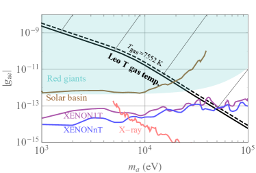
Figure 2: Upper limits on the electron coupling of DM axions. The solid black line is derived from the gas temperature of Leo T by requiring heating rate from DM to be less than the astrophysical cooling rate of the gas. We also show the effect of changing the observational estimate of the gas temperature from $T$=6100 K to the 2$\sigma$ conservative value: $T$=7552 K. Other limits shown in the plot include red giants (cyan) Capozzi and Raffelt (2020), XENON1T (violet) Aprile et al. (2020), XENONnT (blue) Aprile et al. (2022), solar basin (brown) Van Tilburg (2021); Giovanetti et al. (2022) and X-ray (red) Ferreira et al. (2022); Langhoff et al. (2022).

Importantly, we stress that limits from most Earth-based detection experiments (e.g., XENON1T, and also the solar basin limit which is recast from XENON1T) are subject to overburden effects Zaharijas and Farrar (2005) (i.e., if the coupling is too strong, the DM particles will be scattered by the earth’s crust or the atmosphere before they can reach the detectors). Therefore the direct detection limits may not apply to sufficiently large $g_{ae}$. Astrophysical limits naturally evades this limitation and are thus a valuable complement to laboratory limits, excluding the parameter space of large $g_{ae}$. Finally, we remark that the Leo T limit, as well as XENON1T and X-ray limits, require the axions to be DM, whereas stellar cooling and solar basin limits do not rely on the DM assumption.

IV Limits on compact DM

In this section, we constrain various models of compact DM. We first present an overview of models and then study the heating mechanism due to dynamical friction, hard sphere scattering and magnetic charges.

IV.1 Models of compact DM

The landscape of feasible DM masses ranges from $10^{-22}$ eV ultralight bosons to compact objects with mass scales comparable to the Sun. In astrophysics, an important quantity associated with compact objects is the compactness, defined as the ratio of mass to radius. Below we describe four generic classes of compact DM objects in order of decreasing compactness, primordial black holes, composite DM, exotic compact objects and subhalos.

$(i)$ Among all models of compact DM objects, primordial black holes (PBHs) are the most widely studied. PBHs can be created by primordial density fluctuations Zeldovich and Novikov (1967); Hawking (1971); Carr (1975), and if heavy enough ($>10^{15}$ g), they can survive from Hawking evaporation to the present day and behave like DM Chapline (1975). For recent reviews, see e.g., Carr et al. (2016); Green and Kavanagh (2021).

$(ii)$ Composite state of dark sector particles could arise from dark sector interactions, leading to the formation of dark atoms or dark nuclei (see e.g. Wise and Zhang (2014); Chacko et al. (2006); Kaplan et al. (2010, 2011); Chacko et al. (2018); Cline (2021); Krnjaic and Sigurdson (2015); Detmold et al. (2014); Foot and Vagnozzi (2015, 2016)). It is also shown that first-order phase transitions in the early Universe can produce composite DM objects such as quark nuggets Witten (1984); Bai et al. (2019); Hong et al. (2020). Last but not least, composite DM objects could appear as solitons like Q-balls Coleman (1985); Kusenko and Shaposhnikov (1998).

$(iii)$ Exotic compact objects (ECOs) are gravitationally-bound bodies of dark sector particles, stabilized by quantum pressure or self repulsion. The size of an ECO can vary between an asteroid and a star. Boson stars Kaup (1968); Colpi et al. (1986); Eby et al. (2016); Croon et al. (2019), and in particular axion stars Kolb and Tkachev (1993); Visinelli et al. (2018), are well known examples of ECOs. The similar idea has been recently extended to vector bosons Gorghetto et al. (2022). Another possibility for ECO formation is through the complexity in the dark sector. If the dark sector has dissipative interactions similar to SM, there can be viable mechanisms to form mirror stars Mohapatra and Teplitz (1997); Foot et al. (2001); Berezhiani (2004); Curtin and Setford (2020); Hippert et al. (2021) and other ECOs Chang et al. (2019); Dvali et al. (2020).

$(iv)$ DM subhalos are halo-like objects that are spatially more diffuse than ECOs. Many DM models predict the existence of DM subhalos. For example, the smallest possible DM halo is shown to be $10^{-12}$ $M_{\odot}$ Profumo et al. (2006) in WIMP DM models. Models of QCD axions and axion-like particles also predict the formation of miniclusters and minihalos Kolb and Tkachev (1993); Fairbairn et al. (2018); Buschmann et al. (2020); Arvanitaki et al. (2020); Xiao et al. (2021). In early matter domination cosmology, asteroid-mass DM microhalos could be created Nelson and Xiao (2018); Erickcek et al. (2021); Blinov et al. (2021). A final example is ultracompact minihalos surrounding PBHs Ricotti et al. (2008); Eroshenko (2016); Nakama et al. (2019); Hertzberg et al. (2021).

Observational signatures of all these types of compact DM objects can be generally attributed to gravitational and non-gravitational interactions. Gravitational probes include lensing Kolb and Tkachev (1996); Alcock et al. (1998); Niikura et al. (2019, 2019); Witt and Mao (1994); Fairbairn et al. (2017); Bai and Orlofsky (2019); Montero-Camacho et al. (2019); Smyth et al. (2020); Croon et al. (2020a, b); Bai et al. (2020); Fujikura et al. (2021); Dai and Miralda-Escudé (2020); Barnacka et al. (2012); Katz et al. (2018); Ricotti and Gould (2009); Li et al. (2012); Van Tilburg et al. (2018); Mondino et al. (2020), pulsar timing Dror et al. (2019); Ramani et al. (2020), accretion Ali-Haïmoud and Kamionkowski (2017); Bai et al. (2020); Serpico et al. (2020), dynamical friction Carr and Sakellariadou (1999); Brandt (2016); Koushiappas and Loeb (2017); Lu et al. (2021); Takhistov et al. (2021a), and gravitational waves Bird et al. (2016); Giudice et al. (2016); Grabowska et al. (2018); Croon et al. (2019); Hertzberg et al. (2020); Diamond et al. (2021); Marfatia and Tseng (2021); Croon et al. (2022). These probes primarily depend on the mass of compact objects and thus are typically model independent (see however Croon et al. (2020b, a); Bai et al. (2020); Fujikura et al. (2021); Dror et al. (2019); Ramani et al. (2020); Bai et al. (2020); Croon et al. (2022) where dependence on the spatial size of compact objects are investigated). In Sec. IV.3, we will evaluate the sensitivity of dynamical friction constraints to the size of compact objects. On the other hand, depending on the model, compact DM objects could have non-gravitational signatures. For example, they could scatter with SM particles that saturates the geometric cross section Witten (1984); De Rujula and Glashow (1984); Bhoonah et al. (2021); Blanco et al. (2021). In some models, compact DM objects carry charges or couple to photons, allowing them to produce electromagnetic signals Ge et al. (2018); Lehmann et al. (2019); Bai and Orlofsky (2020); Maldacena (2021); Kritos and Silk (2021); Hertzberg et al. (2020); Amin and Mou (2021); Eby et al. (2022).

IV.2 Magnetic primordial black holes

The observed properties of gas in Leo T have been used to constraining in PBHs Lu et al. (2021); Kim (2021); Laha et al. (2020); Takhistov et al. (2021a). BHs passing through Hi  gas can transfer heat to the gas due to various mechanisms like Hawking radiation, dynamical friction, radiation from gas accretion and BH outflows. One can therefore use the cooling rate of gas in Leo T to place limits on heating due to primordial BHs.

In this paper, we focus on magnetically charged BHs. Uncharged BHs below the mass $\sim 10^{15}$g have a lifetime smaller than the age of the Universe (based on their decay via Hawking radiation). Charged BHs, however, stop decaying when they get closer to extremality. Therefore, even very small extremal PBHs can survive until the present.

Primordial BHs with magnetic charges (MBH) can be produced by PBHs absorbing magnetic monopoles in the early universe. Poisson fluctuations in the number density of magnetic monopoles can lead to the PBHs acquiring a net magnetic charge. Note electric charge on a BH can be neutralized by accretion of $e^{+}/e^{-}$ from pairs which are produced in the electric field outside the BH, but magnetic charge cannot be neutralized by accretion of standard model particles. It is worth noting that there are other ways of creating stable charged BHs, in which they are charged under a dark $U$(1) gauge symmetry and the corresponding dark fermion is much heavier than the electron Bai and Orlofsky (2020). Extremal magnetic BHs have been shown to have interesting phenomenological effects Bai et al. (2020); Diamond and Kaplan (2022); Maldacena (2020). The spectrum of quasi-normal modes of such charged BHs has been thoroughly investigated and could be probed with future gravitational wave detectors Zimmerman and Mark (2016); Berti et al. (2009).

We will utilize the fact that compact magnetic objects traveling through astrophysical plasmas get decelerated and transfer heat to the plasmas as a result Meyer-Vernet (1985); Hamilton and Sarazin (1983); Diamond and Kaplan (2022). Diamond and Kaplan (2022) (hereafter D21) recently derived upper bounds on the possible fraction of DM composed of MBHs. They required that the energy deposited by primordial BHs passing through Milky Way Hi  clouds to not exceed their cooling rate. Here, we use the cooling rate of WNM of Leo T to derive a similar constraint on MBHs.

We write the charge of a magnetic BH of mass $M$, in natural units, as Bai et al. (2020); Maldacena (2020)

$$Q\equiv q\,Q_{\mathrm{extremal}}=q\,\sqrt{4\alpha}\frac{M}{M_{\textup{pl}}}$$ (9)

where $M_{\textup{pl}}$ (=1.22$\times 10^{19}$ GeV) is the Planck mass and $q$ is a dimensionless ratio of the BH charge compared to the extremality case.

In Leo T, the velocity of the dipole $v$ is less than the electron thermal velocity of the plasma ($\sqrt{2\,T/m_{e}}$). The heat transferred by an individual object is then given by Meyer-Vernet (1985)

$$\begin{split}\frac{dE}{dt}=&-\frac{4\pi^{1/2}n_{e}}{3\sqrt{2Tm_{e}}}\left[\ln(4\pi n_{e}\lambda^{2}_{D}l)+\frac{2}{3}\right]Q^{2}v^{2}\\ =&-10^{-17}\left(\frac{n_{e}}{\mathrm{cm}^{-3}}\right)\left(\frac{f\,\rho_{\mathrm{DM}}}{\mathrm{GeV}/\mathrm{cm}^{3}}\right)\left(\frac{v}{\mathrm{km/s}}\right)^{2}\\ &\times\left(\frac{q}{1}\right)^{2}\left(\frac{M}{10^{10}\mathrm{g}}\right)\left[\ln(4\pi n_{e}\lambda^{2}_{D}l)+\frac{2}{3}\right]\end{split}$$ (10)

where $n_{e}$ is the electron density, $f$ is the fractional relic density of EMBHs, $\lambda_{D}$ is the Debye length is given by

$$\lambda_{D}=\sqrt{\frac{T}{4\alpha_{\textup{em}}\pi(\sum_{i}Z^{2}_{i}n_{i})}}\,,$$ (11)

and the attenuation length in the plasma is given by

$$l=\left(\frac{2T_{e}}{\pi m_{e}}\right)^{1/4}\frac{1}{v^{1/2}w_{p}}$$ (12)

where $w_{p}=\sqrt{\frac{4\pi n_{e}\alpha}{m_{e}}}$ is the plasma frequency.

We show the bounds from Leo T in Fig. 3 alongside the constraints from Milky Way (MW) clouds by D21. The kinks in the red lines correspond to the case when BHs in the MW halo do not pass through the clouds enough. One advantage that Leo T has over the MW clouds is Hi  is much more widely distributed in it ($r_{\mathrm{WNM}}\sim 0.35$ kpc for Leo T, whereas the clouds used in D21 have sizes $\mathcal{O}$(pc)). Note that the Leo T bound also ultimately cuts off at the point when less than 1 MBH can exist within $r_{\mathrm{WNM}}$, i.e. $f_{\textup{DM}}M_{\mathrm{halo}}<M_{\mathrm{BH}}$ ($M_{\mathrm{halo}}\equiv\int_{0}^{r_{\mathrm{WNM}}}d^{3}r\rho_{\mathrm{DM}}$ is the DM mass enclosed within $r_{\mathrm{WNM}}$). We have also checked that the energy lost by MBHs in Leo T is too small to affect their orbits within the age of the Universe.

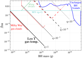
Figure 3: Constraints on fraction of black holes with magnetic charge $q$. charged black holes from the Leo T dwarf galaxy (black), heating of Milky Way’s interstellar medium (ISM) (red) Diamond and Kaplan (2022). Parker bound from the Andromeda galaxy Bai et al. (2020). We also show already existing bounds from Ref. Carr et al. (2021) for uncharged BH that apply to MBHs.

IV.3 Dynamical friction

Dynamical friction (DF) is the effect of the net gravitational interactions from a cloud of lighter bodies on a massive object that is traversing the cloud Chandrasekhar (1943). As a result, the massive traversing object is slowed down and the light bodies in the cloud are accelerated by the gravitational pull. Previously, DF has been used to constrain PBHs traveling in astrophysical environments Carr and Sakellariadou (1999); Brandt (2016); Koushiappas and Loeb (2017); Lu et al. (2021); Takhistov et al. (2021a). The argument is that DF would cause stars in star clusters (or gas particles in interstellar gas) to gain energy and increase their velocity dispersion (or temperature) beyond the observed values. In this section, we generalize the methodology of Refs. Lu et al. (2021); Takhistov et al. (2021a) to study DF constraints on spatially extended compact DM objects using gas temperature of Leo T.

The energy loss rate of a compact DM object with mass $M_{\mathrm{DM}}$ and size $R_{\mathrm{DM}}$ due to DF in a gaseous medium is given by Binney and Tremaine (2008); Ostriker (1999)

$$\derivative{E}{t}=-\frac{4\pi G^{2}M_{\mathrm{DM}}^{2}\rho}{v_{\mathrm{rel}}}I$$ (13)

where $G$ is the gravitational constant, $\rho$ is the gas density and $I$ is the Coulomb logarithm factor. Depending on whether $v_{\mathrm{rel}}$ is larger or smaller than the speed of sound $c_{s}$ in the gas system, $I$ takes the form of

$$I=\Theta(c_{s}-v_{\mathrm{rel}})I_{1}+\Theta(v_{\mathrm{rel}}-c_{s})I_{2},$$ (14)

where $\Theta$ is the Heaviside function, and $I_{1}$ and $I_{2}$ are for the subsonic and supersonic case given respectively by

$$I_{1}=\frac{1}{2}\ln\bigg(\frac{c_{s}+v_{\mathrm{rel}}}{c_{s}-v_{\mathrm{rel}}}\bigg{missing})-\frac{v_{\mathrm{rel}}}{c_{s}},$$ (15)

$$I_{2}=\frac{1}{2}\ln\bigg(1-\frac{c^{2}_{s}}{v_{\mathrm{rel}}^{2}}\bigg{missing})+\ln\bigg(\frac{R_{\mathrm{sys}}}{R_{\mathrm{DM}}}\bigg{missing}),$$

with $R_{\mathrm{sys}}$ characterizing the spatial size of the gas system.

The energy lost by the compact DM object due to DF is directly transferred to the gas. To compute the heating rate on gas, we assume the energy fraction of compact DM objects in the entire halo is $f_{\mathrm{DM}}$, and all of the compact objects have an equal mass $M_{\mathrm{DM}}$ and size $R_{\mathrm{DM}}$ for simplicity. Eq. 13 then leads to the following volume-averaged heating rate

$$\dot{Q}=\frac{12\pi G^{2}f_{\mathrm{DM}}M_{\mathrm{DM}}}{r_{\mathrm{WNM}}^{3}}\int dv_{\mathrm{rel}}dr\,f(v_{\mathrm{rel}})\frac{r^{2}\rho_{\mathrm{DM}}\rho_{\mathrm{H}}}{v_{\mathrm{rel}}}I,$$ (16)

where $\rho_{\mathrm{DM}}$ and $\rho_{\mathrm{H}}$ are the energy density of DM and Hi  respectively. Note that the integration needs to be computed in two parts due to the Heaviside functions in Eq. (14), i.e. an integral in the subsonic regime and another in the supersonic regime. If the DM model features extended distributions of $M_{\mathrm{DM}}$ and $R_{\mathrm{DM}}$, the heating rate in Eq. (16) needs to be weighted by the mass function and size function.

In the left panel of Fig. 4, solid black lines show Leo T gas upper limits on the fraction of compact DM objects. From the thinnest to thickest, we vary $R_{\mathrm{DM}}$ from the Schwarzschild radius to 1 pc. At higher $M_{\mathrm{DM}}$, we also impose the “incredulity” limit following Carr and Sakellariadou (1999); Lu et al. (2021); Takhistov et al. (2021a), which requires $M_{\mathrm{DM}}\leq f_{\mathrm{DM}}M_{\mathrm{halo}}$, where $M_{\mathrm{halo}}=4\pi\int_{0}^{r_{\mathrm{WNM}}}dr\,r^{2}\rho_{\mathrm{DM}}(r)$ is the total DM mass within $r_{\mathrm{WNM}}=0.35$ kpc. Essentially, this condition ensures there is at least one compact DM object in the environment. In this calculation we have adopted the escape velocity $v_{\mathrm{esc}}=23.8$ km/s as discussed in Sec. II. Since this estimation of $v_{\mathrm{esc}}$ is largely conservative, we perform another calculation with $v_{\mathrm{esc}}=62$ km/s to investigate the sensitivity of our results to $v_{\mathrm{esc}}$. We find that the limits are changed by roughly 1% and thus the uncertainty due to $v_{\mathrm{esc}}$ can be neglected. The similar constraint from the MW cloud is shown to be above the $f_{\mathrm{DM}}=1$ baseline Takhistov et al. (2021a) and therefore we do not show it in Fig. 4.

Apart from heating gas in dwarf galaxies, compact DM objects can also heat stellar halos or star clusters via dynamical friction and cause them to expand or dissolve. Properties of the stellar halo of Leo T (e.g., size, mass, age) have been studied in Refs. Simon and Geha (2007); Weisz et al. (2012); Zoutendijk et al. (2021). We use the methodology of Brandt (2016) and require that the timescale to increase the half-light radius $r_{1/2}$ of Leo T by a factor of 2 is longer than the lifetime of the stellar halo; this gives us the limit shown in blue in the left panel of Fig. 4. The details of the calculations are left to Appendix E. The reason for stellar limits in Fig. 4 being stronger than gas limits is that the gas has radiative channels to cool, whereas for the stars, gravitational cooling processes are inefficient Brandt (2016). This is reflected from the fact that gas cooling lifetimes ($\sim 10^{8}$ years for Leo T) are typically much shorter than stellar cooling lifetimes (which are typically expected to be longer than Hubble time).

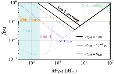
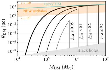
Figure 4: Left: Upper bounds on $f_{\mathrm{DM}}$ as a function of $M_{\mathrm{DM}}$. The black lines are from the gas temperature of Leo T and the thickness of the lines indicate different values of $R_{\mathrm{DM}}$ ranging from the size of black holes to 1 pc. The blue line depicts the limit from the requirement that dynamical heating of stars in Leo T would not increase the half-light radius ($r_{1/2}$) by a factor of two within the stellar halo lifetime. CMB excluded areas Ali-Haïmoud and Kamionkowski (2017) are shown in cyan, Erid II limits Brandt (2016) in violet, the stability of wide binaries Monroy-Rodríguez and Allen (2014) in orange and galactic disks Xu and Ostriker (1994) in green. Right: The sensitivity of Leo T limits to $M_{\mathrm{DM}}$ and $R_{\mathrm{DM}}$. Black contours are constant values of $f_{\mathrm{DM}}$ probed by Leo T constraints. The orange band depicts the relationship of $M_{\mathrm{DM}}$ and $R_{\mathrm{DM}}$ for NFW subhalos with concentration $10^{2}\leq c\leq 10^{5}$, while the cyan line gives the relationship for granular structures in fuzzy DM scenarios Dalal and Kravtsov (2022).

Also shown in Fig. 4 are the excluded regions that overlap with our Leo T limits, from CMB Ali-Haïmoud and Kamionkowski (2017) (cyan), Erid II Brandt (2016) (violet) [see also Zoutendijk et al. (2020)], and the stability of wide binaries Monroy-Rodríguez and Allen (2014) (orange) and galactic disks Xu and Ostriker (1994) (green). All of these bounds are derived for PBHs only, but can be recast for DM objects with larger $R_{\mathrm{DM}}$. The scaling of CMB limits to $R_{\mathrm{DM}}$ has been investigated by Ref. Bai et al. (2020). The Erid II limit is based on DF and therefore we expect similarly weakened limits for larger $R_{\mathrm{DM}}$ as our Leo T limits. For PBHs in this mass range, there are other limits (see e.g. Carr and Sakellariadou (1999); Inoue and Kusenko (2017); Lu et al. (2021); Takhistov et al. (2021b); Bird et al. (2022)) whose generalization to larger $R_{\mathrm{DM}}$ is currently unexplored.. Projections from future astrometric lensing limits will also provide probes into compact DM in this mass range Van Tilburg et al. (2018).

In the right panel of Fig. 4, we calculate the contours of constant $f_{\mathrm{DM}}$ constrained by Leo T gas limits on the $M_{\mathrm{DM}}$-$R_{\mathrm{DM}}$ plane. For example, along the $f_{\mathrm{DM}}\leq 0.1$ contour, compact DM objects with these $M_{\mathrm{DM}}$ and $R_{\mathrm{DM}}$ are constrained by Leo T to make up no more than 10% of the total DM density. The gray region in the bottom indicates the formation of black holes. We also display two exemplary models of DM that feature compact objects and examine if Leo T limits can currently constrain them.

• The orange region shows DM subhalos with an NFW profile with concentration $10^{2}\leq c\leq 10^{5}$. In this scenario, $f_{\mathrm{DM}}$ gives the fraction of DM that forms subhalos. CDM subhalos are typically $10\lesssim c\lesssim 100$ as favored by simulations, and are currently not constrained by Leo T at the level of $f_{\mathrm{DM}}\leq 0.5$. Alternate models such as early matter domination Blinov et al. (2021) and axions Fairbairn et al. (2017) can predict subhalos with much higher concentration, and thus be constrained by Leo T limits. Details about the definition of the mass, size and concentration are given in Appendix C.

• The cyan line corresponds to $M=4\pi\rho_{0}R^{3}/3$ where $\rho_{0}\simeq 1$ GeV/cm ³ is the average DM density in Leo T. Recent studies of fuzzy DM Dalal and Kravtsov (2022) with $m_{a}\sim 10^{-20}$ eV give hints at the formation of granular structures via interference effects. The size of the granule is roughly given by the de Brogile wavelength $R=\order{1}\hbar/(m_{a}\sigma_{v})$ where $\sigma_{v}$ is the 3-dimensional velocity dispersion of DM ($\simeq 7\sqrt{3}$ km/s for Leo T). The mass of the granule is thus $M=4\pi\rho_{0}R^{3}/3$. Each granule would behave as a compact object and the abundance of granules $f_{\mathrm{DM}}$ can be potentially constrained by Leo T. For $m_{a}=10^{-20}$ eV, the characteristic size of the granule is $27$ pc up to an $\order{1}$ proportionality constant, and the characteristic mass is $5\times 10^{3}\,M_{\odot}$ up to the same constant cubed. Currently, these granules are marginally intersecting with the $f_{\mathrm{DM}}\leq 0.2$ contour at $R\sim 100$ pc and $M\sim 10^{6}$-$10^{7}\,M_{\odot}$. Better constraints may be obtained with future study of other gas-rich dwarf galaxies and the improved understanding of granules in fuzzy DM scenarios. It is also worth noting that close to the center of the DM halo (where the Hi  gas is the coldest Adams and Oosterloo (2018)), solitons can produce additional strong dynamical heating, but we have not considered this effect. Apart from the granules heating gas, they can also heat the stellar halo of Leo T. Using the methodology given in Dalal and Kravtsov (2022), observed properties of the stellar halo of Leo T ($\sigma_{*}=7$ km/s and $r_{1/2}\sim 170$ pc Zoutendijk et al. (2021); Simon and Geha (2007)) can be used to add constraints on fuzzy DM in the range $10^{-22}\lesssim m_{\mathrm{FDM}}\lesssim 10^{-20}$ eV.

IV.4 Hard sphere scattering

If non-gravitational interactions between DM and SM exist, more detection strategies become available. To be more specific, we consider heavy DM objects that elastically scatter with SM particles with a cross section set by the geometrical size of DM, $\sigma=\pi R_{\mathrm{DM}}^{2}$. This is similar to the elastic collision of two hard spheres. When DM passes through a medium of density $\rho$ the energy dissipation rate of DM is Opik (1958); De Rujula and Glashow (1984); Bhoonah et al. (2021); Anchordoqui et al. (2021)

$$\derivative{E}{t}=-\rho\sigma v_{\mathrm{rel}}^{3}.$$ (17)

This equation is essentially derived based on the scattering rate $n\sigma v_{\mathrm{rel}}$ and the average energy transfer $\sim mv_{\mathrm{rel}}^{2}$ where $m$ is the particle mass of the medium. Note that the maximum energy transferred is $2mv_{\mathrm{rel}}^{2}$.

In the interstellar gas mediums considered in this paper, the typical number density of hydrogen is $\sim 0.1/\mathrm{cm}^{3}$. The recoiled hydrogen particles from DM-hydrogen collision scatters with other hydrogen with a Rutherford cross section $\sim 10^{-17}\,\mathrm{cm}^{2}$, and therefore the mean free path is $l\sim 1\,\mathrm{pc}$. This is much smaller than the spatial size of the interstellar gas systems that we consider. Therefore, recoiled hydrogen particles can efficiently thermalize with ambient gas particles. Furthermore, because the interstellar gas is sufficiently dilute, the formation of radiation via shock waves De Rujula and Glashow (1984) is highly unlikely in this scenario and we expect that the energy loss Eq. (17) is completely converted to heat.

To compute the heating rate on gas due to hard sphere scattering, we assume that these compact DM objects compose 100% of the DM energy density and they have identical mass $M_{\mathrm{DM}}$ and radius $R_{\mathrm{DM}}$. For Leo T, the volume-averaged heating rate is then

$$\dot{Q}=\frac{\sigma}{M_{\mathrm{DM}}r_{\mathrm{WNM}}^{3}/3}\int dv_{\mathrm{rel}}dr\,v_{\mathrm{rel}}^{3}f(v_{\mathrm{rel}})\rho_{\mathrm{DM}}(r)\rho_{\mathrm{H}}(r).$$ (18)

Similarly, we can calculate the heating rate for the MW cloud. As specified in Sec. II, the Hi  gas density is taken to be a constant $0.4$/cm³. We adopt the NFW profile for the Milky Way DM halo with $\rho_{\chi}=\rho_{0}/[(r/r_{0})(1+r/r_{0})^{2}]$ with $\rho_{0}=0.32$ GeV/cm³, scale radius $r_{0}=16$ kpc and virial radius $180$ kpc Bovy (2015). This gives DM density $\rho_{\mathrm{DM}}=0.64$ GeV/cm³ at the location of the cloud ($r=\sqrt{4.68^{2}+1^{2}}$ kpc). As the heating rate is proportional to $v_{\mathrm{rel}}^{3}$, the MW cloud turns out to set better limits than Leo T due to higher DM velocity dispersion, although Leo T has a smaller cooling rate.

Our results are shown in Fig. 5. The black line depicts the upper limits on $R_{\mathrm{DM}}$ from the MW cloud. A variety of other limits on $R_{\mathrm{DM}}$ are also included. In the lower right corner, the cyan region is ruled out by microlensing ($\mu L$) observation towards M31 Niikura et al. (2019); Croon et al. (2020b) and the black region denotes the formation of black holes. The dashed pink region can be potentially probed by femtolensing (fL) of gamma-ray bursts Jacobs et al. (2015); Barnacka et al. (2012); Katz et al. (2018), but the validity is subject to further investigation of finite-source effects Katz et al. (2018). These bounds are purely gravitational and do not assume a DM-baryon interaction. Other limits are derived from various constraints on DM-baryon scattering cross sections, including CMB (gray) Dvorkin et al. (2014); Jacobs et al. (2015), Mica (orange) Price and Salamon (1986); Jacobs et al. (2015), neutron stars (brown) and white dwarfs (green) Graham et al. (2018); Singh Sidhu and Starkman (2020); Dessert and Johnson (2021), observability of shock waves from DM-star collisions (violet) Das et al. (2021), and lightning (dashed magenta) Sidhu and Starkman (2019); Starkman et al. (2021) (see however Cooray et al. (2021)). We also refer readers to Dhakal et al. (2022) for a new study in using meteor radars to constrain DM-nuclei scattering.

We note that Ref. Bhoonah et al. (2021) reports a similar bound based on another MW-environment gas cloud, G357.8-4.7-55. This gas cloud has a lower cooling rate $3.4\times 10^{-28}$ $\mathrm{erg}\,\mathrm{cm}^{-3}\,\mathrm{s}^{-1}$ and a larger DM density $17$ GeV/cm³ (cf. the cooling rate and DM density for G33.4-8.0 are $2.1\times 10^{-27}$ $\mathrm{erg}\,\mathrm{cm}^{-3}\,\mathrm{s}^{-1}$ and $0.64$ GeV/cm³). In consequence, their limits purport to be stronger than CMB. However, as discussed in Refs. Farrar et al. (2020); Wadekar and Farrar (2021), G357.8-4.7-55 is immersed in an extreme environment (i.e., in the hot and high-velocity outflow from the Galactic Center, with $T_{\mathrm{outflow}}\sim 10^{6-7}$ K), raising questions on if this gas cloud is in a steady state in order to derive constraints on DM heating. We show the close-up of the comparison between these two limits as well as limits from Leo T and self-interacting DM in Appendix D.

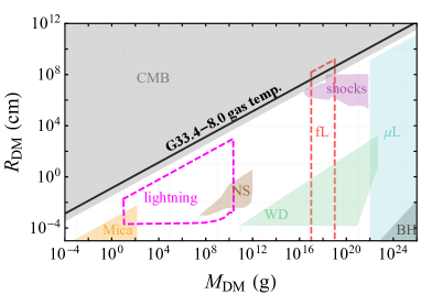
Figure 5: A compilation of constraints on compact DM objects on radius-mass plane. The black line is the upper limit from the gas temperature of a particular Milky Way cloud G33.4$-$8.0. See the text for other bounds.

V Discussion & Conclusions

Observations of cold and metal-poor interstellar gas systems can be a great complement to the program of DM direct and indirect detection. Requiring the heat injection rate from DM lower than the astrophysical cooling rate of the gas can yield compelling limits on a variety of DM models. In this paper, we have derived limits on the following scenarios:
$(i)$ we place upper limits on the electron coupling of axion DM for $m_{a}<100$ keV. This constraint evades the overburden effect that laboratory direct detection experiments suffer from, and rules out the space of large couplings.
$(ii)$ we constrain the abundance of compact DM objects in the mass range $10^{4}\mathrm{-}10^{7}\,M_{\odot}$. We also show the sensitivity to the spatial extent of the compact object. This limit is purely derived from dynamical friction between the compact object and gas and is thus robust for any type of compact objects.
$(iii)$ for DM-nuclei scattering that saturates the geometric cross section, we find upper bounds on the radius of the composite DM state.
$(iv)$ finally, we set upper limits on the abundance of DM in the form magnetically charged black holes.

For calculating the DM bounds from Leo T, we used gas and DM profiles from the model of Leo T by Ref. Faerman et al. (2013). Note however that their model assumes the gas is in hydrostatic equilibrium (i.e., the gravitational force due to the DM halo is balanced by the gas thermal pressure). Their model also does not take into account astrophysical heating and radiative cooling of the Hi  gas. In a future study, we plan to perform hydrodynamic simulations of gas-rich dwarfs like Leo T which include thermal feedback from non-standard DM alongside the standard astrophysical heating and cooling effects. It will also be interesting to perform simulations of Milky Way Hi  clouds including DM heating.

Let us now discuss observational prospects of ultra-faint Hi-rich dwarf galaxies similar to Leo T. Numerous ongoing and upcoming surveys will be able to find and characterize such dwarfs (e.g., 21cm surveys like WALLABY Koribalski et al. (2020), MeerKAT Maddox et al. (2021), Apertif van Cappellen et al. (2022), FAST Zhang et al. (2021), SKA Weltman et al. (2020), and optical surveys like DESI Aghamousa et al. (2016), HSC Aihara et al. (2018), Dragonfly Danieli et al. (2020), Rubin observatory LSST Dark Energy Science Collaboration (2012); Drlica-Wagner et al. (2019); Mutlu-Pakdil et al. (2021), Roman telescope Doré et al. (2018)). Rubin observatory will likely be the most impactful in this regard due to its wide field of view, and its sensitivity to detect dwarfs with brightness similar to Leo T (i.e., $M_{V}=-8$) up to $\sim 5$ Mpc Mutlu-Pakdil et al. (2021). This opens a possibility of detecting hundreds of galaxies similar to Leo T and could enable more stringent probes of heat exchange due to DM.

Appendix A Cooling rates

We had shown the cooling rates of different ISM phases of the Milky Way in Fig. 1. In this Appendix, we discuss the properties of ISM phases used in our cooling rate calculations. We calculate the cooling rate using Eq. 3 and used the properties in Table 1 as input. For the metallicity, we use [Fe/H]$\sim 0$ for all Milky Way systems. It is worth mentioning that the molecular cloud (MC) parameters that we show are for diffuse H₂ systems (the radiative cooling rate is much larger for dense H₂ systems).

Appendix B Axioelectric heating rate

Astrophysical	n	T	Cooling rate
medium	(cm-3)	(K)	(erg cm-3 s-1)
WNM (Leo T)	0.06	6100	$7\times 10^{-30}$
CNM (G33.4$-$8.0)	0.4	400	$1.46\times 10^{-27}$
MC (MW)	100	50	$3.16\times 10^{-24}$
CNM (MW)	30	100	$2.02\times 10^{-24}$
WNM (MW)	0.6	5000	$8.3\times 10^{-27}$
WIM (MW)	0.3	$10^{4}$	$5.4\times 10^{-26}$
HIM (MW)	0.003	106	$1.3\times 10^{-27}$

Table 1: Properties of systems used in calculating the cooling rates shown in Fig. 1. These values are input in Eq. 3 to calculate the cooling rate. The data for different media in the Milky Way (MW) are taken from Table 1.3 of Ref. Draine (2011). The MW phases are labelled as MC (molecular clouds), CNM (cold neutral medium), WNM (warm neutral medium), WIM (warm ionized medium), HIM (hot ionized medium). Note that we only show typical averaged values of the properties of MW phases; these numbers can be different for different systems in a particular phase (e.g., different clouds in WNM of MW can have different properties, e.g., see Lehner et al. (2004)).

In this appendix we give more details of Eq. (7). The radial distribution of DM density and $n_{\mathrm{H}}$ in Leo T are determined by Ref. Faerman et al. (2013) and are plotted by Fig. 1 in Ref. Wadekar and Farrar (2021). For self-contained discussion, we show the Leo T density profile in Fig. 6. The heating efficiency function $f_{e}$ for electrons with kinetic energy $\omega$ takes the form Kim (2021)

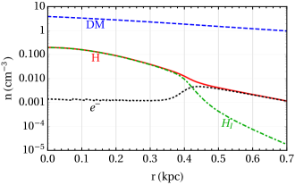
Figure 6: We use a model of the gas-rich Leo T dwarf galaxy by Ref. Faerman et al. (2013), which was fitted to 21cm measurements of the galaxy by Ryan-Weber et al. (2008), and is also consistent with recent stellar velocity dispersion estimates by Zoutendijk et al. (2021). We show the number density of DM (for $m_{\mathrm{DM}}=1$ GeV), atomic hydrogen (Hi), electrons (e^-) and total hydrogen (H) components of the model. This figure is taken from Ref. Wadekar and Farrar (2021) and is shown here for self-contained discussion.

$$\begin{split}f_{e}(\omega)\simeq\,&1-(1-x_{e}^{0.27})^{1.32}\\ &+3.98\bigg{(}\frac{11\mathrm{eV}}{\omega}\bigg{)}^{0.7}x_{e}^{0.4}(1-x_{e}^{0.34})^{2},\end{split}$$ (19)

where $x_{e}=n_{e}/n_{\mathrm{H}}$ is the ionization fraction and in Leo T, $x_{e}\simeq 0.02$.

In the non-relativistic limit, the axioelectric cross section is DIMOPOULOS et al. (1986); Pospelov et al. (2008)

$$\sigma_{ae}=\sigma_{pe}\frac{g_{ae}^{2}}{v_{\mathrm{rel}}}\frac{3m_{a}^{2}}{16\pi\alpha m_{e}^{2}},$$ (20)

where $\sigma_{pe}$ is the the photoelectric cross section of the same atom and $\alpha=1/137$ is the electromagnetic fine structure constant. We obtain $\sigma_{pe}$ of hydrogen from Ref. Veigele (1973) and plot it in Fig. 7.

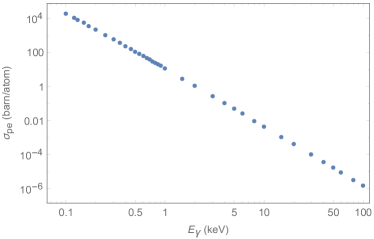
Figure 7: Photoelectric cross section $\sigma_{pe}$ for hydrogen. Data taken from Ref. Veigele (1973).

Note that the inverse proportionality of $\sigma_{pe}$ with $v_{\mathrm{rel}}$ makes the heating rate Eq. (7) independent of $v_{\mathrm{rel}}$. Because of this, Leo T gives stronger limits than the MW cloud.

Appendix C NFW subhalos

We parametrize the density profile of NFW subhalos with scale radius $r_{s}$ and concentration $c$ Ramani et al. (2020)

$$\rho(r)=\frac{200c^{3}\rho_{c}}{3(\ln(1+c)-c/(1+c))}\frac{1}{r/r_{s}(1+r/r_{s})^{2}},$$ (21)

where $\rho_{c}$ is the critical density of the Universe. As the spatial integration of the density is formally divergent, we cut off the profile at $R=100\,r_{s}$ and obtain the mass of the subhalo by $M=4\pi\int_{0}^{100\,r_{s}}dr\,r^{2}\rho(r)$. Based on these we can thus establish the relationship between $M$ and $R$ for fixed values of $c$. We note that in studies of boson stars, the spatial size is often taken to be $R_{90}$ which encloses 90% of the mass. For NFW profile, $R_{90}$ is roughly at $69r_{s}$ and would raise an $\order{1}$ correction to the definition of the size.

Appendix D G357.8-4.7-55 limits on hard sphere scattering

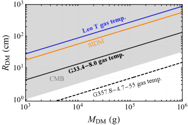
Figure 8: A close-up of Fig. 5 for $M_{\mathrm{DM}}$ between $10^{3}$ and $10^{6}$ g. The orange line corresponds to the upper bound on self-interacting DM cross section $\lesssim 1\,\mathrm{cm}^{2}/\mathrm{g}$ Tulin and Yu (2018).

Fig. 8 shows the close-up of Fig. 5 in the $10^{3}\mathrm{-}10^{6}$ g mass range. The dashed line is recast from the gas heating limit on DM-baryon contact interaction Bhoonah et al. (2021) based on G357.8-4.7-55. As pointed out by Ref. Farrar et al. (2020), this gas cloud is inappropriate for placing limits on DM heat injection. We further display a few additional limits. The blue line shows the limit from Leo T gas temperature with $v_{\mathrm{esc}}=23.8$ km/s. Changing the escape velocity to 62 km/s improves the Leo T limit by roughly 3%. If DM states also self-scatter with a geometrical cross section, the self-interaction is well constrained by astrophysical measurements at the level of $\lesssim 1\,\mathrm{cm}^{2}$ per DM mass in gram Tulin and Yu (2018). This translates to the orange line.

Appendix E Heating of stellar halo in Leo T

In section IV.3, we presented limits from dynamical friction heating of stellar halo of Leo T due to compact DM. Here, we briefly show the steps involved in our calculation of the limits. Note that we have closely followed the methodology of Ref. Brandt (2016) and encourage the reader to refer to their paper for further details. Brandt (2016) derived their limits from heating of a particular stellar cluster at the center of Eridanus II, whereas here we consider heating of the stellar halo in Leo T. Ref. Simon and Geha (2007) fit a Plummer profile to the stellar halo of Leo T and inferred $r_{1/2}=170\pm 15$ pc. Ref. Weisz et al. (2012) estimated that the half of the stellar mass in Leo T formed prior to $7.6$ Gyr, so we use that period as the stellar halo lifetime ($t_{1/2}$) in our calculations.

Due to dynamical friction by compact DM objects, the half-light radius ($r_{1/2}$) of the stellar halo increases at a rate Brandt (2016)

$$\frac{dr_{1/2}}{dt}=\frac{4\sqrt{2}\pi Gf_{\mathrm{DM}}M_{\mathrm{DM}}}{2\beta\sigma_{\mathrm{DM}}r_{1/2}}\ln\Lambda$$ (22)

where $\sigma_{\mathrm{DM}}$ ($M_{\mathrm{DM}}$) is the 3D velocity dispersion (mass) of compact DM objects. $f_{\mathrm{DM}}$ is the fractional contribution of compact objects to the total DM mass density. The Coulomb logarithm is given by Brandt (2016)

$$\ln\Lambda\sim\ln\left(\frac{r_{1/2}\sigma^{2}}{GM_{\mathrm{DM}}}\right)$$ (23)

where we assumed that DM objects are much heavier than stars. We conservatively use $\beta\sim 10$ estimated for a cored Sersic profile Brandt (2016). We require that $r_{1/2}$ to not increase by more than a factor of 2 within the lifetime of Leo T, which gives the following limit on the fraction of DM allowed as compact objects

$$\begin{split}f_{\mathrm{DM}}\lesssim\,&0.02\left(\frac{r_{1/2}}{170\,\mathrm{pc}}\right)^{2}\left(\frac{t_{1/2}}{7.6\,\mathrm{Gyr}}\right)^{-1}\left(\frac{M_{\mathrm{DM}}}{10^{5}\,M_{\odot}}\right)^{-1}\\ &\times\left(\frac{\sigma_{\mathrm{LOS}}}{7.6\,\mathrm{km/s}}\right)\left(\frac{\beta}{10}\right)\left(\frac{\ln\Lambda}{9.86}\right)^{-1}\end{split}$$ (24)

where $\sigma_{\mathrm{LOS}}$ is the 1D velocity dispersion (along line of sight).

References

- Wadekar and Farrar (2021) D. Wadekar and G. R. Farrar, Phys. Rev. D 103, 123028 (2021), arXiv:1903.12190 [hep-ph] .
- Peccei and Quinn (1977) R. D. Peccei and H. R. Quinn, Phys. Rev. D 16, 1791 (1977).
- Weinberg (1978) S. Weinberg, Phys. Rev. Lett. 40, 223 (1978).
- Wilczek (1978) F. Wilczek, Phys. Rev. Lett. 40, 279 (1978).
- Green and Kavanagh (2021) A. M. Green and B. J. Kavanagh, J. Phys. G 48, 043001 (2021), arXiv:2007.10722 [astro-ph.CO] .
- Aprile et al. (2020) E. Aprile et al. (XENON), Phys. Rev. D 102, 072004 (2020), arXiv:2006.09721 [hep-ex] .
- Zaharijas and Farrar (2005) G. Zaharijas and G. R. Farrar, Phys. Rev. D 72, 083502 (2005), arXiv:astro-ph/0406531 .
- Xu et al. (2018) W. L. Xu, C. Dvorkin, and A. Chael, Phys. Rev. D 97, 103530 (2018), arXiv:1802.06788 [astro-ph.CO] .
- Nadler et al. (2019) E. O. Nadler, V. Gluscevic, K. K. Boddy, and R. H. Wechsler, Astrophys. J. Lett. 878, 32 (2019), [Erratum: Astrophys.J.Lett. 897, L46 (2020), Erratum: Astrophys.J. 897, L46 (2020)], arXiv:1904.10000 [astro-ph.CO] .
- Farrar and Zaharijas (2006) G. R. Farrar and G. Zaharijas, Phys. Rev. Lett. 96, 041302 (2006), arXiv:hep-ph/0510079 .
- Leane and Smirnov (2021) R. K. Leane and J. Smirnov, Phys. Rev. Lett. 126, 161101 (2021), arXiv:2010.00015 [hep-ph] .
- Essig et al. (2013) R. Essig, E. Kuflik, S. D. McDermott, T. Volansky, and K. M. Zurek, JHEP 11, 193 (2013), arXiv:1309.4091 [hep-ph] .
- Abdallah et al. (2018) H. Abdallah et al. (HESS), Phys. Rev. Lett. 120, 201101 (2018), arXiv:1805.05741 [astro-ph.HE] .
- Slatyer and Wu (2017) T. R. Slatyer and C.-L. Wu, Phys. Rev. D 95, 023010 (2017), arXiv:1610.06933 [astro-ph.CO] .
- Bolliet et al. (2020) B. Bolliet, J. Chluba, and R. Battye, arXiv e-prints , arXiv:2012.07292 (2020), arXiv:2012.07292 [astro-ph.CO] .
- Ali-Haïmoud (2021) Y. Ali-Haïmoud, Phys. Rev. D 103, 043541 (2021), arXiv:2101.04070 [astro-ph.CO] .
- Bernal et al. (2021) J. L. Bernal, A. Caputo, and M. Kamionkowski, Phys. Rev. D 103, 063523 (2021), arXiv:2012.00771 [astro-ph.CO] .
- Albert et al. (2017) A. Albert et al. (Fermi-LAT, DES), Astrophys. J. 834, 110 (2017), arXiv:1611.03184 [astro-ph.HE] .
- Ando et al. (2020) S. Ando, A. Geringer-Sameth, N. Hiroshima, S. Hoof, R. Trotta, and M. G. Walker, Phys. Rev. D 102, 061302 (2020), arXiv:2002.11956 [astro-ph.CO] .
- Liu et al. (2021) H. Liu, W. Qin, G. W. Ridgway, and T. R. Slatyer, Phys. Rev. D 104, 043514 (2021), arXiv:2008.01084 [astro-ph.CO] .
- Accardo et al. (2014) L. Accardo, M. Aguilar, D. Aisa, B. Alpat, A. Alvino, G. Ambrosi, K. Andeen, L. Arruda, N. Attig, P. Azzarello, A. Bachlechner, F. Barao, A. Barrau, L. Barrin, A. Bartoloni, L. Basara, M. Battarbee, R. Battiston, J. Bazo, U. Becker, M. Behlmann, B. Beischer, J. Berdugo, B. Bertucci, G. Bigongiari, V. Bindi, S. Bizzaglia, M. Bizzarri, G. Boella, W. de Boer, K. Bollweg, V. Bonnivard, B. Borgia, S. Borsini, M. J. Boschini, M. Bourquin, J. Burger, F. Cadoux, X. D. Cai, M. Capell, S. Caroff, G. Carosi, J. Casaus, V. Cascioli, G. Castellini, I. Cernuda, D. Cerreta, F. Cervelli, M. J. Chae, Y. H. Chang, A. I. Chen, H. Chen, G. M. Cheng, H. S. Chen, L. Cheng, A. Chikanian, H. Y. Chou, E. Choumilov, V. Choutko, C. H. Chung, F. Cindolo, C. Clark, R. Clavero, G. Coignet, C. Consolandi, A. Contin, C. Corti, B. Coste, Z. Cui, M. Dai, C. Delgado, S. Della Torre, M. B. Demirköz, L. Derome, S. Di Falco, L. Di Masso, F. Dimiccoli, C. Díaz, P. von Doetinchem, W. J. Du, M. Duranti, D. D’Urso, A. Eline, F. J. Eppling, T. Eronen, Y. Y. Fan, L. Farnesini, J. Feng, E. Fiandrini, A. Fiasson, E. Finch, P. Fisher, Y. Galaktionov, G. Gallucci, B. García, R. García-López, H. Gast, I. Gebauer, M. Gervasi, A. Ghelfi, W. Gillard, F. Giovacchini, P. Goglov, J. Gong, C. Goy, V. Grabski, D. Grandi, M. Graziani, C. Guandalini, I. Guerri, K. H. Guo, D. Haas, M. Habiby, S. Haino, K. C. Han, Z. H. He, M. Heil, R. Henning, J. Hoffman, T. H. Hsieh, Z. C. Huang, C. Huh, M. Incagli, M. Ionica, W. Y. Jang, H. Jinchi, K. Kanishev, G. N. Kim, K. S. Kim, T. Kirn, R. Kossakowski, O. Kounina, A. Kounine, V. Koutsenko, M. S. Krafczyk, S. Kunz, G. La Vacca, E. Laudi, G. Laurenti, I. Lazzizzera, A. Lebedev, H. T. Lee, S. C. Lee, C. Leluc, G. Levi, H. L. Li, J. Q. Li, Q. Li, Q. Li, T. X. Li, W. Li, Y. Li, Z. H. Li, Z. Y. Li, S. Lim, C. H. Lin, P. Lipari, T. Lippert, D. Liu, H. Liu, M. Lolli, T. Lomtadze, M. J. Lu, Y. S. Lu, K. Luebelsmeyer, F. Luo, J. Z. Luo, S. S. Lv, R. Majka, A. Malinin, C. Mañá, J. Marín, T. Martin, G. Martínez, N. Masi, F. Massera, D. Maurin, A. Menchaca-Rocha, Q. Meng, D. C. Mo, B. Monreal, L. Morescalchi, P. Mott, M. Müller, J. Q. Ni, N. Nikonov, F. Nozzoli, P. Nunes, A. Obermeier, A. Oliva, M. Orcinha, F. Palmonari, C. Palomares, M. Paniccia, A. Papi, M. Pauluzzi, E. Pedreschi, S. Pensotti, R. Pereira, R. Pilastrini, F. Pilo, A. Piluso, C. Pizzolotto, V. Plyaskin, M. Pohl, V. Poireau, E. Postaci, A. Putze, L. Quadrani, X. M. Qi, P. G. Rancoita, D. Rapin, J. S. Ricol, I. Rodríguez, S. Rosier-Lees, L. Rossi, A. Rozhkov, D. Rozza, G. Rybka, R. Sagdeev, J. Sandweiss, P. Saouter, C. Sbarra, S. Schael, S. M. Schmidt, D. Schuckardt, A. Schulz von Dratzig, G. Schwering, G. Scolieri, E. S. Seo, B. S. Shan, Y. H. Shan, J. Y. Shi, X. Y. Shi, Y. M. Shi, T. Siedenburg, D. Son, F. Spada, F. Spinella, W. Sun, W. H. Sun, M. Tacconi, C. P. Tang, X. W. Tang, Z. C. Tang, L. Tao, D. Tescaro, S. C. C. Ting, S. M. Ting, N. Tomassetti, J. Torsti, C. Türkoğlu, T. Urban, V. Vagelli, E. Valente, C. Vannini, E. Valtonen, S. Vaurynovich, M. Vecchi, M. Velasco, J. P. Vialle, V. Vitale, G. Volpini, L. Q. Wang, Q. L. Wang, R. S. Wang, X. Wang, Z. X. Wang, Z. L. Weng, K. Whitman, J. Wienkenhöver, H. Wu, K. Y. Wu, X. Xia, M. Xie, S. Xie, R. Q. Xiong, G. M. Xin, N. S. Xu, W. Xu, Q. Yan, J. Yang, M. Yang, Q. H. Ye, H. Yi, Y. J. Yu, Z. Q. Yu, S. Zeissler, J. H. Zhang, M. T. Zhang, X. B. Zhang, Z. Zhang, Z. M. Zheng, F. Zhou, H. L. Zhuang, V. Zhukov, A. Zichichi, N. Zimmermann, P. Zuccon, and C. Zurbach (AMS Collaboration), Phys. Rev. Lett. 113, 121101 (2014).
- Chivukula et al. (1990) S. R. Chivukula, A. G. Cohen, S. Dimopoulos, and T. P. Walker, Phys. Rev. Lett. 65, 957 (1990).
- Dubovsky and Hernández-Chifflet (2015) S. Dubovsky and G. Hernández-Chifflet, Journal of Cosmology and Astro-Particle Physics 2015, 054 (2015), arXiv:1509.00039 [hep-ph] .
- Bhoonah et al. (2018) A. Bhoonah, J. Bramante, F. Elahi, and S. Schon, Phys. Rev. Lett. 121, 131101 (2018), arXiv:1806.06857 [hep-ph] .
- Bhoonah et al. (2018) A. Bhoonah, J. Bramante, F. Elahi, and S. Schon, arXiv e-prints (2018), arXiv:1812.10919 [hep-ph] .
- Bhoonah et al. (2021) A. Bhoonah, J. Bramante, S. Schon, and N. Song, Phys. Rev. D 103, 123026 (2021), arXiv:2010.07240 [hep-ph] .
- Farrar et al. (2020) G. R. Farrar, F. J. Lockman, N. M. McClure-Griffiths, and D. Wadekar, Phys. Rev. Lett. 124, 029001 (2020), arXiv:1903.12191 [hep-ph] .
- Lu et al. (2021) P. Lu, V. Takhistov, G. B. Gelmini, K. Hayashi, Y. Inoue, and A. Kusenko, ApJ 908, L23 (2021), arXiv:2007.02213 [astro-ph.CO] .
- Laha et al. (2020) R. Laha, P. Lu, and V. Takhistov, arXiv e-prints , arXiv:2009.11837 (2020), arXiv:2009.11837 [astro-ph.CO] .
- Kim (2021) H. Kim, MNRAS 504, 5475 (2021), arXiv:2007.07739 [hep-ph] .
- Takhistov et al. (2021a) V. Takhistov, P. Lu, G. B. Gelmini, K. Hayashi, Y. Inoue, and A. Kusenko, arXiv e-prints , arXiv:2105.06099 (2021a), arXiv:2105.06099 [astro-ph.GA] .
- Takhistov et al. (2021b) V. Takhistov, P. Lu, K. Murase, Y. Inoue, and G. B. Gelmini, arXiv e-prints , arXiv:2111.08699 (2021b), arXiv:2111.08699 [astro-ph.HE] .
- Wadekar and Wang (2022) D. Wadekar and Z. Wang, Phys. Rev. D 106, 075007 (2022), arXiv:2111.08025 [hep-ph] .
- Diamond and Kaplan (2022) M. D. Diamond and D. E. Kaplan, JHEP 03, 157 (2022), arXiv:2103.01850 [hep-ph] .
- Draine (2011) B. T. Draine, Physics of the Interstellar and Intergalactic Medium (2011).
- Ryan-Weber et al. (2008) E. V. Ryan-Weber, A. Begum, T. Oosterloo, S. Pal, M. J. Irwin, V. Belokurov, N. W. Evans, and D. B. Zucker, MNRAS 384, 535 (2008), arXiv:0711.2979 .
- Adams and Oosterloo (2018) E. A. K. Adams and T. A. Oosterloo, A&A 612, A26 (2018), arXiv:1712.06636 .
- Faerman et al. (2013) Y. Faerman, A. Sternberg, and C. F. McKee, Astrophys. J. 777, 119 (2013), arXiv:1309.0815 [astro-ph.CO] .
- Burkert (1995) A. Burkert, ApJ 447, L25 (1995), arXiv:astro-ph/9504041 [astro-ph] .
- Smith et al. (2017) B. D. Smith, G. L. Bryan, S. C. O. Glover, N. J. Goldbaum, M. J. Turk, J. Regan, J. H. Wise, H.-Y. Schive, T. Abel, A. Emerick, B. W. O’Shea, P. Anninos, C. B. Hummels, and S. Khochfar, MNRAS 466, 2217 (2017), arXiv:1610.09591 .
- Zoutendijk et al. (2021) S. L. Zoutendijk, M. P. Júlio, J. Brinchmann, J. I. Read, D. Vaz, L. A. Boogaard, N. F. Bouché, D. Krajnović, K. Kuijken, J. Schaye, and M. Steinmetz, arXiv e-prints , arXiv:2112.09374 (2021), arXiv:2112.09374 [astro-ph.GA] .
- Simon and Geha (2007) J. D. Simon and M. Geha, ApJ 670, 313 (2007), arXiv:0706.0516 .
- Piffl et al. (2014) T. Piffl et al., Astron. Astrophys. 562, A91 (2014), arXiv:1309.4293 [astro-ph.GA] .
- Pidopryhora et al. (2015) Y. Pidopryhora, F. J. Lockman, J. M. Dickey, and M. P. Rupen, ApJS 219, 16 (2015), arXiv:1506.03873 [astro-ph.GA] .
- DIMOPOULOS et al. (1986) S. DIMOPOULOS, G. D. STARKMAN, and B. W. LYNN, Modern Physics Letters A 01, 491 (1986), https://doi.org/10.1142/S0217732386000622 .
- Pospelov et al. (2008) M. Pospelov, A. Ritz, and M. Voloshin, Phys. Rev. D 78, 115012 (2008).
- Ferreira et al. (2022) R. Z. Ferreira, M. C. D. Marsh, and E. Müller, (2022), arXiv:2202.08858 [hep-ph] .
- Capozzi and Raffelt (2020) F. Capozzi and G. Raffelt, Phys. Rev. D 102, 083007 (2020), arXiv:2007.03694 [astro-ph.SR] .
- Aprile et al. (2022) E. Aprile et al. (XENON), (2022), arXiv:2207.11330 [hep-ex] .
- Van Tilburg (2021) K. Van Tilburg, Phys. Rev. D 104, 023019 (2021), arXiv:2006.12431 [hep-ph] .
- Giovanetti et al. (2022) C. Giovanetti, R. Lasenby, and K. Van Tilburg, (2022).
- Langhoff et al. (2022) K. Langhoff, N. J. Outmezguine, and N. L. Rodd, Phys. Rev. Lett. 129, 241101 (2022), arXiv:2209.06216 [hep-ph] .
- O’Hare (2020) C. O’Hare, “cajohare/axionlimits: Axionlimits,” https://cajohare.github.io/AxionLimits/ (2020).
- Adams et al. (2022) C. B. Adams et al., in 2022 Snowmass Summer Study (2022) arXiv:2203.14923 [hep-ex] .
- Foster et al. (2022) J. W. Foster, S. Kumar, B. R. Safdi, and Y. Soreq, (2022), arXiv:2208.10504 [hep-ph] .
- Lee et al. (2014) H. M. Lee, S. C. Park, and W.-I. Park, Eur. Phys. J. C 74, 3062 (2014), arXiv:1403.0865 [astro-ph.CO] .
- Zeldovich and Novikov (1967) Y. B. Zeldovich and I. D. Novikov, Soviet Astron. AJ (Engl. Transl.), 10: 602-3(Jan.-Feb. 1967). (1967).
- Hawking (1971) S. Hawking, Monthly Notices of the Royal Astronomical Society 152, 75 (1971), https://academic.oup.com/mnras/article-pdf/152/1/75/9360899/mnras152-0075.pdf .
- Carr (1975) B. J. Carr, ApJ 201, 1 (1975).
- Chapline (1975) G. F. Chapline, Nature 253, 251 (1975).
- Carr et al. (2016) B. Carr, F. Kuhnel, and M. Sandstad, Phys. Rev. D 94, 083504 (2016), arXiv:1607.06077 [astro-ph.CO] .
- Wise and Zhang (2014) M. B. Wise and Y. Zhang, Phys. Rev. D 90, 055030 (2014), [Erratum: Phys.Rev.D 91, 039907 (2015)], arXiv:1407.4121 [hep-ph] .
- Chacko et al. (2006) Z. Chacko, H.-S. Goh, and R. Harnik, Phys. Rev. Lett. 96, 231802 (2006), arXiv:hep-ph/0506256 .
- Kaplan et al. (2010) D. E. Kaplan, G. Z. Krnjaic, K. R. Rehermann, and C. M. Wells, JCAP 05, 021 (2010), arXiv:0909.0753 [hep-ph] .
- Kaplan et al. (2011) D. E. Kaplan, G. Z. Krnjaic, K. R. Rehermann, and C. M. Wells, JCAP 10, 011 (2011), arXiv:1105.2073 [hep-ph] .
- Chacko et al. (2018) Z. Chacko, D. Curtin, M. Geller, and Y. Tsai, JHEP 09, 163 (2018), arXiv:1803.03263 [hep-ph] .
- Cline (2021) J. M. Cline, in Les Houches summer school on Dark Matter (2021) arXiv:2108.10314 [hep-ph] .
- Krnjaic and Sigurdson (2015) G. Krnjaic and K. Sigurdson, Phys. Lett. B 751, 464 (2015), arXiv:1406.1171 [hep-ph] .
- Detmold et al. (2014) W. Detmold, M. McCullough, and A. Pochinsky, Phys. Rev. D 90, 115013 (2014), arXiv:1406.2276 [hep-ph] .
- Foot and Vagnozzi (2015) R. Foot and S. Vagnozzi, Phys. Rev. D 91, 023512 (2015), arXiv:1409.7174 [hep-ph] .
- Foot and Vagnozzi (2016) R. Foot and S. Vagnozzi, JCAP 07, 013 (2016), arXiv:1602.02467 [astro-ph.CO] .
- Witten (1984) E. Witten, Phys. Rev. D 30, 272 (1984).
- Bai et al. (2019) Y. Bai, A. J. Long, and S. Lu, Phys. Rev. D 99, 055047 (2019), arXiv:1810.04360 [hep-ph] .
- Hong et al. (2020) J.-P. Hong, S. Jung, and K.-P. Xie, Phys. Rev. D 102, 075028 (2020), arXiv:2008.04430 [hep-ph] .
- Coleman (1985) S. R. Coleman, Nucl. Phys. B 262, 263 (1985), [Addendum: Nucl.Phys.B 269, 744 (1986)].
- Kusenko and Shaposhnikov (1998) A. Kusenko and M. E. Shaposhnikov, Phys. Lett. B 418, 46 (1998), arXiv:hep-ph/9709492 .
- Kaup (1968) D. J. Kaup, Phys. Rev. 172, 1331 (1968).
- Colpi et al. (1986) M. Colpi, S. L. Shapiro, and I. Wasserman, Phys. Rev. Lett. 57, 2485 (1986).
- Eby et al. (2016) J. Eby, C. Kouvaris, N. G. Nielsen, and L. C. R. Wijewardhana, JHEP 02, 028 (2016), arXiv:1511.04474 [hep-ph] .
- Croon et al. (2019) D. Croon, J. Fan, and C. Sun, JCAP 04, 008 (2019), arXiv:1810.01420 [hep-ph] .
- Kolb and Tkachev (1993) E. W. Kolb and I. I. Tkachev, Phys. Rev. Lett. 71, 3051 (1993), arXiv:hep-ph/9303313 .
- Visinelli et al. (2018) L. Visinelli, S. Baum, J. Redondo, K. Freese, and F. Wilczek, Phys. Lett. B 777, 64 (2018), arXiv:1710.08910 [astro-ph.CO] .
- Gorghetto et al. (2022) M. Gorghetto, E. Hardy, J. March-Russell, N. Song, and S. M. West, (2022), arXiv:2203.10100 [hep-ph] .
- Mohapatra and Teplitz (1997) R. N. Mohapatra and V. L. Teplitz, Astrophys. J. 478, 29 (1997), arXiv:astro-ph/9603049 .
- Foot et al. (2001) R. Foot, A. Y. Ignatiev, and R. R. Volkas, Phys. Lett. B 503, 355 (2001), arXiv:astro-ph/0011156 .
- Berezhiani (2004) Z. Berezhiani, Int. J. Mod. Phys. A 19, 3775 (2004), arXiv:hep-ph/0312335 .
- Curtin and Setford (2020) D. Curtin and J. Setford, JHEP 03, 041 (2020), arXiv:1909.04072 [hep-ph] .
- Hippert et al. (2021) M. Hippert, J. Setford, H. Tan, D. Curtin, J. Noronha-Hostler, and N. Yunes, (2021), arXiv:2103.01965 [astro-ph.HE] .
- Chang et al. (2019) J. H. Chang, D. Egana-Ugrinovic, R. Essig, and C. Kouvaris, JCAP 03, 036 (2019), arXiv:1812.07000 [hep-ph] .
- Dvali et al. (2020) G. Dvali, E. Koutsangelas, and F. Kuhnel, Phys. Rev. D 101, 083533 (2020), arXiv:1911.13281 [astro-ph.CO] .
- Profumo et al. (2006) S. Profumo, K. Sigurdson, and M. Kamionkowski, Phys. Rev. Lett. 97, 031301 (2006), arXiv:astro-ph/0603373 .
- Fairbairn et al. (2018) M. Fairbairn, D. J. E. Marsh, J. Quevillon, and S. Rozier, Phys. Rev. D 97, 083502 (2018), arXiv:1707.03310 [astro-ph.CO] .
- Buschmann et al. (2020) M. Buschmann, J. W. Foster, and B. R. Safdi, Phys. Rev. Lett. 124, 161103 (2020), arXiv:1906.00967 [astro-ph.CO] .
- Arvanitaki et al. (2020) A. Arvanitaki, S. Dimopoulos, M. Galanis, L. Lehner, J. O. Thompson, and K. Van Tilburg, Phys. Rev. D 101, 083014 (2020), arXiv:1909.11665 [astro-ph.CO] .
- Xiao et al. (2021) H. Xiao, I. Williams, and M. McQuinn, Phys. Rev. D 104, 023515 (2021), arXiv:2101.04177 [astro-ph.CO] .
- Nelson and Xiao (2018) A. E. Nelson and H. Xiao, Phys. Rev. D 98, 063516 (2018), arXiv:1807.07176 [astro-ph.CO] .
- Erickcek et al. (2021) A. L. Erickcek, P. Ralegankar, and J. Shelton, Phys. Rev. D 103, 103508 (2021), arXiv:2008.04311 [astro-ph.CO] .
- Blinov et al. (2021) N. Blinov, M. J. Dolan, P. Draper, and J. Shelton, Phys. Rev. D 103, 103514 (2021), arXiv:2102.05070 [astro-ph.CO] .
- Ricotti et al. (2008) M. Ricotti, J. P. Ostriker, and K. J. Mack, Astrophys. J. 680, 829 (2008), arXiv:0709.0524 [astro-ph] .
- Eroshenko (2016) Y. N. Eroshenko, Astron. Lett. 42, 347 (2016), arXiv:1607.00612 [astro-ph.HE] .
- Nakama et al. (2019) T. Nakama, K. Kohri, and J. Silk, Phys. Rev. D 99, 123530 (2019), arXiv:1905.04477 [astro-ph.CO] .
- Hertzberg et al. (2021) M. P. Hertzberg, S. Nurmi, E. D. Schiappacasse, and T. T. Yanagida, Phys. Rev. D 103, 063025 (2021), arXiv:2011.05922 [hep-ph] .
- Kolb and Tkachev (1996) E. W. Kolb and I. I. Tkachev, Astrophys. J. Lett. 460, L25 (1996), arXiv:astro-ph/9510043 .
- Alcock et al. (1998) C. Alcock et al. (MACHO, EROS), Astrophys. J. Lett. 499, L9 (1998), arXiv:astro-ph/9803082 .
- Niikura et al. (2019) H. Niikura et al., Nature Astron. 3, 524 (2019), arXiv:1701.02151 [astro-ph.CO] .
- Witt and Mao (1994) H. J. Witt and S. Mao, ApJ 430, 505 (1994).
- Fairbairn et al. (2017) M. Fairbairn, D. J. E. Marsh, and J. Quevillon, Phys. Rev. Lett. 119, 021101 (2017), arXiv:1701.04787 [astro-ph.CO] .
- Bai and Orlofsky (2019) Y. Bai and N. Orlofsky, Phys. Rev. D 99, 123019 (2019), arXiv:1812.01427 [astro-ph.HE] .
- Montero-Camacho et al. (2019) P. Montero-Camacho, X. Fang, G. Vasquez, M. Silva, and C. M. Hirata, JCAP 08, 031 (2019), arXiv:1906.05950 [astro-ph.CO] .
- Smyth et al. (2020) N. Smyth, S. Profumo, S. English, T. Jeltema, K. McKinnon, and P. Guhathakurta, Phys. Rev. D 101, 063005 (2020), arXiv:1910.01285 [astro-ph.CO] .
- Croon et al. (2020a) D. Croon, D. McKeen, and N. Raj, Phys. Rev. D 101, 083013 (2020a), arXiv:2002.08962 [astro-ph.CO] .
- Croon et al. (2020b) D. Croon, D. McKeen, N. Raj, and Z. Wang, Phys. Rev. D 102, 083021 (2020b), arXiv:2007.12697 [astro-ph.CO] .
- Bai et al. (2020) Y. Bai, A. J. Long, and S. Lu, JCAP 09, 044 (2020), arXiv:2003.13182 [astro-ph.CO] .
- Fujikura et al. (2021) K. Fujikura, M. P. Hertzberg, E. D. Schiappacasse, and M. Yamaguchi, Phys. Rev. D 104, 123012 (2021), arXiv:2109.04283 [hep-ph] .
- Dai and Miralda-Escudé (2020) L. Dai and J. Miralda-Escudé, Astron. J. 159, 49 (2020), arXiv:1908.01773 [astro-ph.CO] .
- Barnacka et al. (2012) A. Barnacka, J. F. Glicenstein, and R. Moderski, Phys. Rev. D 86, 043001 (2012), arXiv:1204.2056 [astro-ph.CO] .
- Katz et al. (2018) A. Katz, J. Kopp, S. Sibiryakov, and W. Xue, JCAP 12, 005 (2018), arXiv:1807.11495 [astro-ph.CO] .
- Ricotti and Gould (2009) M. Ricotti and A. Gould, Astrophys. J. 707, 979 (2009), arXiv:0908.0735 [astro-ph.CO] .
- Li et al. (2012) F. Li, A. L. Erickcek, and N. M. Law, Phys. Rev. D 86, 043519 (2012), arXiv:1202.1284 [astro-ph.CO] .
- Van Tilburg et al. (2018) K. Van Tilburg, A.-M. Taki, and N. Weiner, JCAP 07, 041 (2018), arXiv:1804.01991 [astro-ph.CO] .
- Mondino et al. (2020) C. Mondino, A.-M. Taki, K. Van Tilburg, and N. Weiner, Phys. Rev. Lett. 125, 111101 (2020), arXiv:2002.01938 [astro-ph.CO] .
- Dror et al. (2019) J. A. Dror, H. Ramani, T. Trickle, and K. M. Zurek, Phys. Rev. D 100, 023003 (2019), arXiv:1901.04490 [astro-ph.CO] .
- Ramani et al. (2020) H. Ramani, T. Trickle, and K. M. Zurek, JCAP 12, 033 (2020), arXiv:2005.03030 [astro-ph.CO] .
- Ali-Haïmoud and Kamionkowski (2017) Y. Ali-Haïmoud and M. Kamionkowski, Phys. Rev. D 95, 043534 (2017), arXiv:1612.05644 [astro-ph.CO] .
- Serpico et al. (2020) P. D. Serpico, V. Poulin, D. Inman, and K. Kohri, Phys. Rev. Res. 2, 023204 (2020), arXiv:2002.10771 [astro-ph.CO] .
- Carr and Sakellariadou (1999) B. J. Carr and M. Sakellariadou, The Astrophysical Journal 516, 195 (1999).
- Brandt (2016) T. D. Brandt, Astrophys. J. Lett. 824, L31 (2016), arXiv:1605.03665 [astro-ph.GA] .
- Koushiappas and Loeb (2017) S. M. Koushiappas and A. Loeb, Phys. Rev. Lett. 119, 041102 (2017), arXiv:1704.01668 [astro-ph.GA] .
- Lu et al. (2021) P. Lu, V. Takhistov, G. B. Gelmini, K. Hayashi, Y. Inoue, and A. Kusenko, Astrophys. J. Lett. 908, L23 (2021), arXiv:2007.02213 [astro-ph.CO] .
- Bird et al. (2016) S. Bird, I. Cholis, J. B. Muñoz, Y. Ali-Haïmoud, M. Kamionkowski, E. D. Kovetz, A. Raccanelli, and A. G. Riess, Phys. Rev. Lett. 116, 201301 (2016), arXiv:1603.00464 [astro-ph.CO] .
- Giudice et al. (2016) G. F. Giudice, M. McCullough, and A. Urbano, JCAP 10, 001 (2016), arXiv:1605.01209 [hep-ph] .
- Grabowska et al. (2018) D. M. Grabowska, T. Melia, and S. Rajendran, Phys. Rev. D 98, 115020 (2018), arXiv:1807.03788 [hep-ph] .
- Hertzberg et al. (2020) M. P. Hertzberg, Y. Li, and E. D. Schiappacasse, JCAP 07, 067 (2020), arXiv:2005.02405 [hep-ph] .
- Diamond et al. (2021) M. D. Diamond, D. E. Kaplan, and S. Rajendran, (2021), arXiv:2112.09147 [hep-ph] .
- Marfatia and Tseng (2021) D. Marfatia and P.-Y. Tseng, JHEP 11, 068 (2021), arXiv:2107.00859 [hep-ph] .
- Croon et al. (2022) D. Croon, S. Ipek, and D. McKeen, (2022), arXiv:2205.15396 [astro-ph.CO] .
- De Rujula and Glashow (1984) A. De Rujula and S. L. Glashow, Nature 312, 734 (1984).
- Blanco et al. (2021) C. Blanco, B. Elshimy, R. F. Lang, and R. Orlando, (2021), arXiv:2112.14784 [hep-ph] .
- Ge et al. (2018) S. Ge, X. Liang, and A. Zhitnitsky, Phys. Rev. D 97, 043008 (2018), arXiv:1711.06271 [hep-ph] .
- Lehmann et al. (2019) B. V. Lehmann, C. Johnson, S. Profumo, and T. Schwemberger, JCAP 10, 046 (2019), arXiv:1906.06348 [hep-ph] .
- Bai and Orlofsky (2020) Y. Bai and N. Orlofsky, Phys. Rev. D 101, 055006 (2020), arXiv:1906.04858 [hep-ph] .
- Maldacena (2021) J. Maldacena, JHEP 04, 079 (2021), arXiv:2004.06084 [hep-th] .
- Kritos and Silk (2021) K. Kritos and J. Silk, (2021), arXiv:2109.09769 [gr-qc] .
- Amin and Mou (2021) M. A. Amin and Z.-G. Mou, JCAP 02, 024 (2021), arXiv:2009.11337 [astro-ph.CO] .
- Eby et al. (2022) J. Eby, S. Shirai, Y. V. Stadnik, and V. Takhistov, Phys. Lett. B 825, 136858 (2022), arXiv:2106.14893 [hep-ph] .
- Bai et al. (2020) Y. Bai, J. Berger, M. Korwar, and N. Orlofsky, Journal of High Energy Physics 2020, 210 (2020), arXiv:2007.03703 [hep-ph] .
- Maldacena (2020) J. Maldacena, arXiv e-prints , arXiv:2004.06084 (2020), arXiv:2004.06084 [hep-th] .
- Zimmerman and Mark (2016) A. Zimmerman and Z. Mark, Phys. Rev. D 93, 044033 (2016), arXiv:1512.02247 [gr-qc] .
- Berti et al. (2009) E. Berti, V. Cardoso, and A. O. Starinets, Classical and Quantum Gravity 26, 163001 (2009), arXiv:0905.2975 [gr-qc] .
- Meyer-Vernet (1985) N. Meyer-Vernet, ApJ 290, 21 (1985).
- Hamilton and Sarazin (1983) A. J. S. Hamilton and C. L. Sarazin, ApJ 274, 399 (1983).
- Carr et al. (2021) B. Carr, K. Kohri, Y. Sendouda, and J. Yokoyama, Reports on Progress in Physics 84, 116902 (2021), arXiv:2002.12778 [astro-ph.CO] .
- Chandrasekhar (1943) S. Chandrasekhar, ApJ 97, 255 (1943).
- Binney and Tremaine (2008) J. Binney and S. Tremaine, Galactic Dynamics: Second Edition (2008).
- Ostriker (1999) E. C. Ostriker, Astrophys. J. 513, 252 (1999), arXiv:astro-ph/9810324 .
- Weisz et al. (2012) D. R. Weisz, D. B. Zucker, A. E. Dolphin, N. F. Martin, J. T. A. de Jong, J. A. Holtzman, J. J. Dalcanton, K. M. Gilbert, B. F. Williams, E. F. Bell, V. Belokurov, and N. W. Evans, ApJ 748, 88 (2012), arXiv:1201.4859 .
- Monroy-Rodríguez and Allen (2014) M. A. Monroy-Rodríguez and C. Allen, ApJ 790, 159 (2014), arXiv:1406.5169 [astro-ph.GA] .
- Xu and Ostriker (1994) G. Xu and J. P. Ostriker, ApJ 437, 184 (1994).
- Dalal and Kravtsov (2022) N. Dalal and A. Kravtsov, Phys. Rev. D 106, 063517 (2022), arXiv:2203.05750 [astro-ph.CO] .
- Zoutendijk et al. (2020) S. L. Zoutendijk, J. Brinchmann, L. A. Boogaard, M. L. P. Gunawardhana, T.-O. Husser, S. Kamann, A. F. Ramos Padilla, M. M. Roth, R. Bacon, M. den Brok, S. Dreizler, and D. Krajnović, A&A 635, A107 (2020), arXiv:2001.08790 [astro-ph.GA] .
- Inoue and Kusenko (2017) Y. Inoue and A. Kusenko, JCAP 10, 034 (2017), arXiv:1705.00791 [astro-ph.CO] .
- Bird et al. (2022) S. Bird et al., (2022), arXiv:2203.08967 [hep-ph] .
- Opik (1958) E. J. Opik, Physics of meteor flight in the atmosphere. (1958).
- Anchordoqui et al. (2021) L. A. Anchordoqui et al., Europhys. Lett. 135, 51001 (2021), arXiv:2104.05131 [hep-ph] .
- Bovy (2015) J. Bovy, ApJS 216, 29 (2015), arXiv:1412.3451 .
- Jacobs et al. (2015) D. M. Jacobs, G. D. Starkman, and B. W. Lynn, Mon. Not. Roy. Astron. Soc. 450, 3418 (2015), arXiv:1410.2236 [astro-ph.CO] .
- Dvorkin et al. (2014) C. Dvorkin, K. Blum, and M. Kamionkowski, Phys. Rev. D 89, 023519 (2014), arXiv:1311.2937 [astro-ph.CO] .
- Price and Salamon (1986) P. B. Price and M. H. Salamon, Phys. Rev. Lett. 56, 1226 (1986).
- Graham et al. (2018) P. W. Graham, R. Janish, V. Narayan, S. Rajendran, and P. Riggins, Phys. Rev. D 98, 115027 (2018), arXiv:1805.07381 [hep-ph] .
- Singh Sidhu and Starkman (2020) J. Singh Sidhu and G. D. Starkman, Phys. Rev. D 101, 083503 (2020), arXiv:1912.04053 [astro-ph.CO] .
- Dessert and Johnson (2021) C. Dessert and Z. Johnson, (2021), arXiv:2112.06949 [hep-ph] .
- Das et al. (2021) A. Das, S. A. R. Ellis, P. C. Schuster, and K. Zhou, (2021), arXiv:2106.09033 [hep-ph] .
- Sidhu and Starkman (2019) J. S. Sidhu and G. Starkman, Phys. Rev. D 100, 123008 (2019), arXiv:1908.00557 [astro-ph.CO] .
- Starkman et al. (2021) N. Starkman, J. Sidhu, H. Winch, and G. Starkman, Phys. Rev. D 103, 063024 (2021), arXiv:2006.16272 [astro-ph.CO] .
- Cooray et al. (2021) V. Cooray, G. Cooray, M. Rubinstein, and F. Rachidi, (2021), 10.3390/atmos12091230, arXiv:2107.05338 [physics.ao-ph] .
- Dhakal et al. (2022) P. Dhakal, S. Prohira, C. V. Cappiello, J. F. Beacom, S. Palo, and J. Marino, (2022), arXiv:2209.07690 [hep-ph] .
- Koribalski et al. (2020) B. S. Koribalski et al., Ap&SS 365, 118 (2020), arXiv:2002.07311 [astro-ph.GA] .
- Maddox et al. (2021) N. Maddox et al., A&A 646, A35 (2021), arXiv:2011.09470 [astro-ph.GA] .
- van Cappellen et al. (2022) W. A. van Cappellen et al., A&A 658, A146 (2022), arXiv:2109.14234 [astro-ph.IM] .
- Zhang et al. (2021) K. Zhang, J. Wu, D. Li, C.-W. Tsai, L. Staveley-Smith, J. Wang, J. Fu, T. McIntyre, and M. Yuan, MNRAS 500, 1741 (2021), arXiv:2012.01683 [astro-ph.GA] .
- Weltman et al. (2020) A. Weltman et al., PASA 37, e002 (2020), arXiv:1810.02680 [astro-ph.CO] .
- Aghamousa et al. (2016) A. Aghamousa et al. (DESI), (2016), arXiv:1611.00036 [astro-ph.IM] .
- Aihara et al. (2018) H. Aihara et al., PASJ 70, S4 (2018), arXiv:1704.05858 [astro-ph.IM] .
- Danieli et al. (2020) S. Danieli, D. Lokhorst, J. Zhang, A. Merritt, P. van Dokkum, R. Abraham, C. Conroy, C. Gilhuly, J. Greco, S. Janssens, J. Li, Q. Liu, T. B. Miller, and L. Mowla, ApJ 894, 119 (2020), arXiv:1910.14045 [astro-ph.GA] .
- LSST Dark Energy Science Collaboration (2012) LSST Dark Energy Science Collaboration, arXiv e-prints , arXiv:1211.0310 (2012), arXiv:1211.0310 [astro-ph.CO] .
- Drlica-Wagner et al. (2019) A. Drlica-Wagner et al., arXiv e-prints , arXiv:1902.01055 (2019), arXiv:1902.01055 [astro-ph.CO] .
- Mutlu-Pakdil et al. (2021) B. Mutlu-Pakdil, D. J. Sand, D. Crnojević, A. Drlica-Wagner, N. Caldwell, P. Guhathakurta, A. C. Seth, J. D. Simon, J. Strader, and E. Toloba, arXiv e-prints , arXiv:2105.01658 (2021), arXiv:2105.01658 [astro-ph.GA] .
- Doré et al. (2018) O. Doré et al. (WFIRST), (2018), arXiv:1804.03628 [astro-ph.CO] .
- Lehner et al. (2004) N. Lehner, B. P. Wakker, and B. D. Savage, ApJ 615, 767 (2004), arXiv:astro-ph/0407363 [astro-ph] .
- Veigele (1973) W. Veigele, Atomic Data and Nuclear Data Tables 5, 51 (1973).
- Tulin and Yu (2018) S. Tulin and H.-B. Yu, Phys. Rept. 730, 1 (2018), arXiv:1705.02358 [hep-ph] .