The photon energy spectrum in $B\to X_{s}\gamma$ at N³LL^′

Abstract

We present predictions for the photon energy spectrum in inclusive $B\to X_{s}\gamma$ decays mediated by the electromagnetic penguin operator $O_{7}$ to N³LL^′. We use soft-collinear effective theory (SCET) to resum the singular contributions in the peak region at large photon energy. In the tail region the resummed predictions are matched to fixed order at N³LO, where we include the known fixed-order contributions for $O_{7}$ up to $\mathcal{O}(\alpha_{s}^{2})$. We develop a method to suitably parametrize the still unknown $\mathcal{O}(\alpha_{s}^{3})$ nonsingular corrections in terms of theory nuisance parameters, whose variations provide an estimate of the associated theory uncertainty. In this context, we also study different ways to treat higher-order cross terms in the matching. Another important aspect of our analysis is the short-distance scheme used for the $b$-quark mass $m_{b}$. We find that in the present context, the 1$S$ mass scheme, which was previously used up to 2-loop order, fails to work at 3-loop order, because the mass scheme enters at a soft scale much smaller than $m_{b}$ here, for which the 1$S$ scheme was not devised. Using instead the MSR mass scheme with $R\sim 1\,\mathrm{GeV}$, we obtain stable results with good perturbative convergence up to N³LL^′.

1 Introduction

The flavor-changing neutral-current $b\to s\gamma$ transition plays a key role in exploring the flavor sector of the Standard Model (SM) [1, 2, 3, 4] and in searches for possible physics beyond the SM [5, 6, 7]. A prominent example is the inclusive $B\to X_{s}\gamma$ decay, whose normalization is sensitive to beyond-SM contributions.

Experimental measurements of $B\to X_{s}\gamma$ are most sensitive in the peak region at large photon energy $E_{\gamma}$, where as a result also most information on the normalization of the $B\to X_{s}\gamma$ rate comes from. Furthermore, the shape of the $E_{\gamma}$ spectrum is directly sensitive to the $b$-quark distribution function, known as shape function, which describes the relevant nonperturbative dynamics of the $b$ quark within the $B$ meson [8, 9, 10]. Recently, the first global fit exploiting all available experimental information on the $B\to X_{s}\gamma$ spectrum [11, 12, 13, 14] was carried out by the SIMBA collaboration [15], simultaneously extracting the normalization of the $B\to X_{s}\gamma$ rate, encoded in the effective inclusive Wilson coefficient $C_{7}^{\rm incl}$, the $b$-quark mass $m_{b}$, as well as the shape function.

The shape function is a universal object that also enters the description of inclusive $B\to X_{u}\ell\nu$ [9, 10, 16] and $B\to X_{s}\ell^{+}\ell^{-}$ [17, 18] decays, where one restricts the phase space to small hadronic invariant masses to suppress the otherwise overwhelmingly large background from $b\to c\ell\nu$ transitions. In particular, it enters in the extraction of the Cabibbo-Kobayashi-Maskawa (CKM) matrix element $|V_{ub}|$ from $B\to X_{u}\ell\nu$, which is important for overconstraining the flavor sector of the SM as it is one of the few tree-level quantities. Inclusive determinations of $|V_{ub}|$ show some tensions with its determination from exclusive decays as well as the indirect determination from the CKM unitarity [19].

In the analysis of ref. [15], the theoretical predictions for the $B\to X_{s}\gamma$ spectrum are obtained at NNLL${}^{\prime}+$NNLO. The final fit results exhibit a similar size of theoretical and experimental uncertainties. On the experimental side, upcoming and future Belle II measurements [20, 21] of $B\to X_{s}\gamma$ and $B\to X_{u}\ell\nu$ will further reduce the experimental uncertainties. To benefit from the improved experimental precision, the theoretical predictions have to be improved likewise.

In this work, we take an important step in this direction by extending the resummed predictions to the next order, N³LL^′, taking advantage of the recent computation of the 3-loop jet function and heavy-to-light soft function [22, 23]. At this order, the 3-loop hard function, corresponding to the $b\to s\gamma$ form factor, is also needed but currently not known. Therefore, in our numerical results, we treat its unknown nonlogarithmic constant term at $\mathcal{O}(\alpha_{s}^{3})$ as a theory nuisance parameter [24, 25] which we vary as part of our perturbative uncertainties.

To obtain a complete description of the spectrum away from the endpoint, we have to match to the full fixed-order result. At N³LL^′, this requires one to perform the matching to N³LO. Since the full fixed-order results at this order are not known, we devise a method to parametrize the missing ingredients in terms of a set of theory nuisance parameters $c_{k}$ [24, 25] in such a way that the matching can be performed in a consistent manner and the perturbative uncertainties due to the missing ingredients can be estimated. We denote the so-constructed matched result as N³LL${}^{\prime}+$N³LO$(c_{k})$. It provides a description of the $B\to X_{s}\gamma$ spectrum which benefits from the improved precision at N³LL^′ in the peak region while consistently including the known fixed-order results up to $\mathcal{O}(\alpha_{s}^{2})$ [26, 27, 28].

Throughout the paper, we focus on the contributions from the electromagnetic penguin operator, $O_{7}$, in the electroweak Hamiltonian, which induces the to-be-resummed singular contributions that dominate at large photon energies. At sufficiently high order, operators other than $O_{7}$ also produce singular contributions, but these are always $O_{7}$-like and are automatically included via the definition of $C_{7}^{\rm incl}$. The purely nonsingular contributions from non-$O_{7}$ operators can simply be added to the order they are known as in ref. [15], so we do not discuss them here further.

Extending the resummation order to N³LL^′ turns out to be more subtle than one might naively expect. We find that the 1$S$ mass scheme [29, 30, 31], which was used at NNLL^′ in refs. [32, 15], fails to provide a stable prediction at N³LL^′. The cause for this failure lies in the intrinsic scale $R^{1S}(\mu_{S})$ of the 1$S$ scheme, which at the soft scale $\mu_{S}$ becomes large and incompatible with the power counting of HQET. On the other hand, by using the MSR scheme [33] we are able to obtain stable predictions that exhibit good perturbative convergence. Furthermore, at N³LL^′ it turns out to become necessary to switch to a short-distance mass scheme also in the jet and hard functions, which makes the RGE of the hard function more involved, where $m_{b}$ plays the role of setting the hard kinematic scale.

The outline of this paper is as follows. In section 2 we present our theory framework and discuss all the ingredients for computing the $B\to X_{s}\gamma$ photon energy spectrum at N³LL${}^{\prime}+$N³LO$(c_{k})$. We discuss the implementation of the short-distance mass scheme in more detail in section 3. Our methodology for estimating the perturbative uncertainties of our predictions is given in section 4. In section 5, we present our numerical results and discuss alternative choices for the $b$-quark mass scheme and the treatment of higher-order perturbative terms. We summarize our findings in section 6.

2 Theory framework

2.1 Overview

We follow the setup of ref. [15] and write the $B\to X_{s}\gamma$ photon energy spectrum as

$$\frac{\mathrm{d}\Gamma}{\mathrm{d}E_{\gamma}}=2\Gamma_{0}\biggl{(}\frac{2E_{\gamma}}{\widehat{m}_{b}}\biggr{)}^{3}\int\!\mathrm{d}k\,\widehat{P}(k)\,\mathcal{F}(m_{B}-2E_{\gamma}-k)+\mathcal{O}\biggl{(}\frac{\Lambda_{\rm QCD}}{\widehat{m}_{b}}\biggr{)}\,,$$ (2.1)

where $\widehat{m}_{b}$ denotes the $b$-quark mass in a short-distance scheme and

$$\Gamma_{0}=\frac{G_{F}^{2}\,\widehat{m}_{b}^{5}}{8\pi^{3}}\frac{\alpha_{\rm em}}{4\pi}|V_{tb}V_{ts}^{*}|^{2}\,.$$ (2.2)

The function $\widehat{P}(k)$ is perturbatively calculable and corresponds to the partonic $b\to s\gamma$ spectrum with $k\sim\widehat{m}_{b}-2E_{\gamma}$. We write it as [15]

$$\widehat{P}(k)=\bigl{|}C_{7}^{\rm incl}\bigr{|}^{2}\Bigl{[}W_{77}^{\rm s}(k)+W_{77}^{\rm ns}(k)\Bigr{]}+2\operatorname{Re}(C_{7}^{\rm incl})\sum_{i\neq 7}\mathcal{C}_{i}W_{7i}^{\rm ns}(k)+\sum_{i,j\neq 7}\mathcal{C}_{i}\mathcal{C}_{j}W_{ij}^{\rm ns}(k)\,.$$ (2.3)

The coefficient $C_{7}^{\rm incl}$ contains by definition all virtual contributions from operators in the electroweak Hamiltonian that give rise to singular contributions [34, 15]. It is dominated by the Wilson coefficient $C_{7}$ of the electromagnetic operator $O_{7}$. In this paper, we focus on the contributions proportional to $\bigl{|}C_{7}^{\rm incl}\bigr{|}^{2}$, which are discussed in more detail in the following.

The function $W_{77}^{\rm s}(k)$ in eq. (2.3) accounts for the contributions to the partonic spectrum $\sim\delta(k)$ and $\ln^{n}(k/\widehat{m}_{b})/k$ that are singular and dominant in the peak of the spectrum where $k\ll\widehat{m}_{b}$. They can be resummed to all orders based on their well-known factorization [35, 36]. We will resum them to N³LL^′, as discussed in more detail in section 2.2. Note that the overall factor $(2E_{\gamma}/\widehat{m}_{b})^{3}$ in eq. (2.1) has a purely kinematic origin. It arises from the photon phase space integration and derivative operators in the photon field strength tensor of $O_{7}$. As in ref. [15], we factor it out of the singular contributions and keep it unexpanded in the endpoint region.

The function $W_{77}^{\rm ns}(k)$ in eq. (2.3) contains the remaining nonsingular contributions to the partonic spectrum. They start at $\mathcal{O}(\alpha_{s})$ and are accompanied by powers of $k/\widehat{m}_{b}$ relative to the singular contributions in $W_{77}^{\mathrm{s}}$. Thus, they are power-suppressed in the peak region where $k\ll\widehat{m}_{b}$. On the other hand, in the tail region where $k\sim\widehat{m}_{b}$, they are of similar size as the singular contributions. We will include their known results at fixed order to $\mathcal{O}(\alpha_{s}^{2})$, while the currently unknown corrections at $\mathcal{O}(\alpha_{s}^{3})$ are estimated by introducing appropriate theory nuisance parameters, as discussed in section 2.3.

The remaining non-77 contributions $W_{i7}^{\mathrm{ns}}$ and $W_{ij}^{\mathrm{ns}}$ in eq. (2.3) are purely nonsingular and thus only become relevant in the tail region. Since they do not have singular counterparts, they can be straightforwardly added to the order they are known, as was done in ref. [15]. We neglect them in the following, since our focus here is on the resummation and fixed-order matching of the dominant 77 contributions. Similarly, we neglect the remaining $\mathcal{O}(\Lambda_{\rm QCD}/\widehat{m}_{b})$ terms in eq. (2.1), which contain subdominant resolved and unresolved contributions.

To ensure that eq. (2.1) reproduces the full fixed-order result in the tail with a smooth transition between the peak and tail regimes, we use profile scales to gradually switch off the resummation away from the peak region, as discussed in section 2.4.

The nonperturbative function $\mathcal{F}(k)$ in eq. (2.1) contains the leading shape function as well as the combination of subleading shape functions that appear at tree level in $B\to X_{s}\gamma$. It is discussed in section 2.5. The partonic spectrum $\widehat{P}$ and the hadronic shape function $\mathcal{F}$ are completely factorized in eq. (2.1). This factorization enables a coherent description of the spectrum in both peak and tail region. In the tail region only the first few moments of $\mathcal{F}$ are relevant, while in the peak region its full form is required.

2.2 Singular contributions

The singular contributions $W_{77}^{\mathrm{s}}(k)$ are the leading contributions to the spectrum in the limit $k\ll m_{b}$. Their well-known factorization theorem [35, 36] allows us to systematically resum the large logarithmic distributions to all orders in perturbation theory. Here we make use of the SCET-based factorization theorem following ref. [32]

$$W_{77}^{\rm s}(k) =\widehat{h}_{s}(\widehat{m}_{b},\mu_{H})\,\widehat{U}_{H}(\widehat{m}_{b},\mu_{H},\mu_{J})\times$$

$$\quad\times\int\!\mathrm{d}\omega\,\mathrm{d}\omega^{\prime}\,\widehat{m}_{b}\,\widehat{J}(\widehat{m}_{b}(k-\omega),\mu_{J})\,U_{S}(\omega-\omega^{\prime},\mu_{S},\mu_{J})\,\widehat{C}_{0}(\omega^{\prime},\mu_{S})\,,$$ (2.4)

where $\widehat{h}_{s}$, $\widehat{J}$, and $\widehat{C}_{0}$ are the hard, jet, and partonic soft functions, respectively. The hard and soft evolution kernels, $\widehat{U}_{H}$ and $U_{S}$, evolve the hard and soft functions from their characteristic hard and soft scales, $\mu_{H}$ and $\mu_{S}$, to the jet scale, $\mu_{J}$, thereby summing logarithms of the form $\ln(\mu_{H}/\mu_{J})$ and $\ln(\mu_{J}/\mu_{S})$. Since we choose to evolve everything to the jet scale, the jet evolution kernel $\widehat{U}_{J}(p^{2},\mu_{J},\mu_{J})=\delta(p^{2})$ drops out. The hats indicate that an object is defined in a renormalon-free short-distance scheme, as discussed in more detail in section 3. Explicit results for the perturbative ingredients are collected in appendix A.

In eq. (2.2), $\widehat{h}_{s}(\mu_{H})$, $\widehat{J}(\mu_{J})$, $\widehat{C}_{0}(\mu_{S})$ are the boundary conditions for the evolution, which are evaluated at fixed order. When doing so, by default we always strictly reexpand their product to the given order in $\alpha_{s}$, i.e., we count $\alpha_{s}(\mu_{H})\sim\alpha_{s}(\mu_{J})\sim\alpha_{s}(\mu_{S})$ and drop all higher-order cross terms in the product of their fixed-order series. By doing so, the strict fixed-order expansion of $W_{77}^{\mathrm{s}}$ in terms of a common $\alpha_{s}(\mu)$ is reproduced simply by taking all scales to be equal $\mu_{H}=\mu_{J}=\mu_{S}=\mu$. This is different to refs. [32, 15], where only the product $\widehat{J}\otimes\widehat{C}_{0}$ is reexpanded, while the hard function is kept unexpanded as an overall multiplicative factor, which results in keeping certain higher-order cross terms in the fixed-order limit. The effect of these differences is studied in section 5.2.

To resum the singular corrections using eq. (2.2) to N³LL^′ order, we have to include the fixed-order boundary conditions $\widehat{h}_{s}(\mu_{H})$, $\widehat{J}(\mu_{J})$, $\widehat{C}_{0}(\mu_{S})$ to $\mathcal{O}(\alpha_{s}^{3})$ and use the 3-loop noncusp and $4$-loop cusp anomalous dimensions as well as the $4$-loop beta function in the evolution factors $\widehat{U}_{H}(\mu_{H},\mu_{J})$ and $U_{S}(\mu_{J},\mu_{S})$. The jet and soft functions have been computed up to three loops in refs. [16, 37, 22] and refs. [16, 38, 23], respectively.

Regarding the hard function, its 3-loop anomalous dimension is also known via the consistency relation with the jet and soft anomalous dimensions and is given in ref. [23]. The full hard function is currently only known up to NNLO [39, 32]. We account for all the logarithmic terms at N³LO, which are determined using the RGE in terms of the known anomalous dimensions and lower-order constant terms. The result is given in appendix A.2. Thus, the only missing ingredient to obtain $W_{77}^{\rm s}$ at full $\rm N^{3}LL^{\prime}$ is the finite, nonlogarithmic 3-loop constant of the hard function, $h_{3}$, which is defined by expanding the (pole-scheme) hard function at $\mu=m_{b}$ as

$$h_{s}(m_{b},\mu_{H}=m_{b})=1+\frac{\alpha_{s}(m_{b})}{\pi}\,h_{1}+\frac{\alpha_{s}^{2}(m_{b})}{\pi^{2}}\,h_{2}+\frac{\alpha_{s}^{3}(m_{b})}{\pi^{3}}\,h_{3}+\mathcal{O}(\alpha_{s}^{4})\,.$$ (2.5)

We treat this unknown constant as a theory nuisance parameter,

$$h_{3}=0\pm 80\,,$$ (2.6)

where the range of variation is estimated using the Padé approximation

$$h_{3}\sim\frac{h_{2}^{2}}{\lvert h_{1}\rvert}\sim\frac{19.3^{2}}{4.55}\sim 80\,.$$ (2.7)

We will see in section 5 that it only has a minor impact on the perturbative precision of our results.

For future reference, we write the fixed-order expansion of the singular contribution up to ${\rm N^{3}LO}$ as

$$W_{77}^{\rm s}(\widehat{m}_{b}x) =\frac{C_{F}}{\widehat{m}_{b}}\biggl{\{}w^{\mathrm{s}(0)}_{77}(x)+\frac{\alpha_{s}(\mu)}{\pi}\bigl{[}w^{\mathrm{s}(1)}_{77}(x)+\Delta w^{\mathrm{s}(1)}_{77}(\mu,x)\bigr{]}$$

$$\quad\qquad+\frac{\alpha_{s}^{2}(\mu)}{\pi^{2}}\biggl{[}w^{\mathrm{s}(2)}_{77}(x)+\frac{\beta_{0}}{2}w^{\mathrm{s}(1)}_{77}(x)\ln\frac{\mu}{\widehat{m}_{b}}+\Delta w^{\mathrm{s}(2)}_{77}(\mu,x)\biggr{]}$$

$$\quad\qquad+\frac{\alpha_{s}^{3}(\mu)}{\pi^{3}}\biggl{[}w^{\mathrm{s}(3)}_{77}(x)+\biggl{(}\beta_{0}w^{\mathrm{s}(2)}_{77}(x)+\frac{\beta_{1}}{8}w^{\mathrm{s}(1)}_{77}(x)\biggr{)}\ln\frac{\mu}{\widehat{m}_{b}}$$

$$\qquad\qquad\qquad\quad+\frac{\beta_{0}^{2}}{4}w^{\mathrm{s}(1)}_{77}(x)\ln^{2}\frac{\mu}{\widehat{m}_{b}}+\Delta w^{\mathrm{s}(3)}_{77}(\mu,x)\biggr{]}+\mathcal{O}(\alpha_{s}^{4})\biggr{\}}\,,$$ (2.8)

where we have made the fixed-order $\mu$ dependence and its order-by-order cancellation explicit. Numerically, we have

$$w^{\mathrm{s}(0)}_{77}(x) =0.75\,\delta(x)\,,$$

$$w^{\mathrm{s}(1)}_{77}(x) =-4.54\,\delta(x)-1.75\,\mathcal{L}_{0}(x)-1.00\,\mathcal{L}_{1}(x)\,,$$

$$w^{\mathrm{s}(2)}_{77}(x) =(-30.5+3.01\,n_{f})\,\delta(x)+(5.94+0.316\,n_{f})\,\mathcal{L}_{0}(x)+(12.4-0.181\,n_{f})\,\mathcal{L}_{1}(x)$$

$$\quad+(7.63-0.250\,n_{f})\,\mathcal{L}_{2}(x)+0.667\,\mathcal{L}_{3}(x)\,,$$

$$w^{\mathrm{s}(3)}_{77}(x) =(88.2+0.75h_{3}-0.0269\,n_{f}-0.0309\,n_{f}^{2})\,\delta(x)$$ (2.9)

$$\quad+(138-9.16\,n_{f}-0.00330\,n_{f}^{2})\,\mathcal{L}_{0}(x)$$

$$\quad+(68.7-8.75\,n_{f}+0.121\,n_{f}^{2})\,\mathcal{L}_{1}(x)+(-25.1-0.815\,n_{f}+0.00694\,n_{f}^{2})\,\mathcal{L}_{2}(x)$$

$$\quad+(-43.0+3.16\,n_{f}-0.0648\,n_{f}^{2})\mathcal{L}_{3}(x)+(-6.53+0.278\,n_{f})\mathcal{L}_{4}(x)-0.222\,\mathcal{L}_{5}(x)\,,$$

where $\mathcal{L}_{n}(x)\equiv[\ln^{n}(x)/x]_{+}$ are the usual plus distributions defined in eq. (A.1). Note that at this order the unknown 3-loop constant $h_{3}$ appears only in the $\delta(x)$ coefficient, so $w^{\mathrm{s}(3)}_{77}(x)$ is completely known for $x>0$.

The correction terms $\Delta w_{77}^{\mathrm{s}(n)}(\mu,x)$ in eq. (2.2) arise from switching to the short-distance $b$-quark mass $\widehat{m}_{b}$, and their $\mu$ dependence separately cancels among them order by order. They are discussed in more detail in section 3.4, and their explicit expressions are provided in eq. (3.4).

2.3 Nonsingular contributions

The nonsingular contribution $W_{77}^{\mathrm{ns}}(k)$ is included at fixed order. It is obtained by subtracting the fixed-order singular terms from the full fixed-order result for $\mathrm{d}\Gamma/\mathrm{d}E_{\gamma}$, which is known up to $\mathcal{O}(\alpha_{s}^{2})$ [26, 27, 28]. We write its perturbative expansion up to $\rm N^{3}LO$ as

$$W_{77}^{\rm ns}(\widehat{m}_{b}x) =\frac{C_{F}}{\widehat{m}_{b}(1-x)^{3}}\biggl{\{}\frac{\alpha_{s}(\mu_{\rm ns})}{\pi}\,w^{{\rm ns}(1)}_{77}(x)$$

$$\quad+\frac{\alpha_{s}^{2}(\mu_{\rm ns})}{\pi^{2}}\biggl{[}w^{{\rm ns}(2)}_{77}(x)+\frac{\beta_{0}}{2}\,w^{{\rm ns}(1)}_{77}(x)\,\ln\frac{\mu_{\rm ns}}{\widehat{m}_{b}}+\Delta w^{{\rm ns}(2)}_{77}(\mu_{\rm ns},x)\biggr{]}$$

$$\quad+\frac{\alpha_{s}^{3}(\mu_{\rm ns})}{\pi^{3}}\biggl{[}w^{{\rm ns}(3)}_{77}(x)+\biggl{(}\beta_{0}w^{{\rm ns}(2)}_{77}(x)+\frac{\beta_{1}}{8}w^{{\rm ns}(1)}_{77}(x)\biggr{)}\ln\frac{\mu_{\rm ns}}{\widehat{m}_{b}}$$

$$\qquad\qquad\qquad+\frac{\beta_{0}^{2}}{4}\,w^{{\rm ns}(1)}_{77}(x)\ln^{2}\frac{\mu_{\rm ns}}{\widehat{m}_{b}}+\Delta w^{{\rm ns}(3)}_{77}(\mu_{\rm ns},x)\biggr{]}\biggr{\}}\,.$$ (2.10)

The overall $1/(1-x)^{3}$ factor is included by convention. Explicit expressions for $w^{{\rm ns}(1)}_{77}(x)$ and $w^{{\rm ns}(2)}_{77}(x)$ are given in eq. (S21) in ref. [15]. The $\mathcal{O}(\alpha_{s}^{3})$ function $w^{{\rm ns}(3)}_{77}(x)$ is currently unknown. The $\Delta w^{\mathrm{ns}(n)}_{77}(\mu_{\mathrm{ns}},x)$ terms arise from switching to the short-distance mass $\widehat{m}_{b}$ and are given in eq. (3.4).

In the peak region for $k\ll\widehat{m}_{b}$, the nonsingular are power-suppressed by $k/\widehat{m}_{b}$ relative to the singular. Hence, the two can be considered as independent perturbative series, which are treated separately from each other. In particular, it is consistent to include the nonsingular only at fixed order, while the singular are being resummed. By contrast, for $k\sim\widehat{m}_{b}$, the separation into singular and nonsingular becomes ill-defined and only the full result given by their sum, $W_{77}^{\mathrm{full}}=W_{77}^{\mathrm{s}}+W_{77}^{\mathrm{ns}}$, is meaningful. This is reflected by the fact that there are typically large numerical cancellations between the singular and nonsingular contributions for $k\to\widehat{m}_{b}$, as we will see explicitly in section 2.4. Consequently, $W_{77}^{\mathrm{s}}$ and $W_{77}^{\mathrm{ns}}$ must be included using the same perturbative expansion in this limit, i.e., at the same scale and the same perturbative order, to ensure that the cancellations between them can take place and the proper full result is recovered. This has important ramifications. First, since the full and nonsingular results are only known at fixed order, it is essential to turn off the resummation for $W_{77}^{\mathrm{s}}$ for $k\sim\widehat{m}_{b}$ such that it also reduces to its fixed-order result. Second, the NⁿLL^′ resummation reduces to the fixed $\mathcal{O}(\alpha_{s}^{n})$ singular result, so consistently matching it to fixed order requires including the nonsingular to $\mathcal{O}(\alpha_{s}^{n})$.

Therefore, at N³LL^′ we need $W_{77}^{\mathrm{ns}}$ to $\mathcal{O}(\alpha_{s}^{3})$, which means we have to parametrize the unknown nonsingular function $w^{{\rm ns}(3)}_{77}(x)$. We do so by considering its required asymptotic behavior in the $x\to 0$ and $x\to 1$ limits. In particular, for $x\to 1$ we have to account for the singular-nonsingular cancellations at $\mathcal{O}(\alpha_{s}^{3})$, which basically implies that $w_{77}^{\mathrm{ns}(3)}$ and $w_{77}^{\mathrm{s}(3)}$ are not independent. In addition, we want to exploit the parameterization to estimate the perturbative uncertainty due to the missing $w^{\mathrm{ns}(3)}_{77}(x)$.

We begin by separating $w^{\mathrm{ns}(3)}_{77}(x)$ into a “correlated” and an “uncorrelated” piece,

$$w^{{\rm ns}(3)}_{77}(x)=w^{{\rm ns}(3)}_{\rm cor}(x)+w^{{\rm ns}(3)}_{\rm uncor}(x)\,.$$ (2.11)

The “correlated” term $w^{{\rm ns}(3)}_{\rm cor}(x)$ is designed to completely cancel the singular corrections in the $x\to 1$ limit without disturbing the hierarchy between singular and nonsingular contributions in the $x\to 0$ limit. We define it as

$$w^{{\rm ns}(3)}_{\rm cor}(x)=-(1-x)^{3}\,w^{{\rm s}(3)}_{77}(1)\,,$$ (2.12)

where the 3-loop singular function $w^{{\rm s}(3)}_{77}(x)$ is defined in eq. (2.2). The overall factor $(1-x)^{3}$ simply cancels the overall $1/(1-x)^{3}$ in eq. (2.3). The remaining “uncorrelated” piece $w^{{\rm ns}(3)}_{\rm uncor}(x)$ can now be considered independent of the singular contribution, so we can parametrize it. We do so by expanding it as

$$w^{{\rm ns}(3)}_{\rm uncor}(x)=(1-x)^{3}\,\sum_{k=0}^{5}\,c_{k}^{\rm ns}\,L^{k}(x)\qquad\text{with}\qquad L(x)=\frac{1}{4}\frac{w^{{\rm ns}(1)}_{77}(x)}{(1-x)^{3}}-\frac{9}{16}\,,$$ (2.13)

where the function $L(x)$ is positive for $0<x<1$ and has the following asymptotics in the $x\to 0$ and $x\to 1$ limits,

$$L(x) =-\frac{3}{2}-\ln x+\mathcal{O}(x)\,, L(x) =0+\mathcal{O}(1-x)\,.$$ (2.14)

We construct $L(x)$ using $w^{{\rm ns}(1)}_{77}(x)$ with the expectation that its powers provide a reasonable guess of the possible shape of the higher-order function $w^{{\rm ns}(3)}_{77}(x)$ in the intermediate region $0<x<1$. Furthermore, eq. (2.13) incorporates the knowledge that at $\mathcal{O}(\alpha_{s}^{3})$ the nonsingular in the limit $x\to 0$ is a degree-5 polynomial in $\ln x$. Therefore we include up to five powers of $L(x)$ to ensure we are able to probe the complete logarithmic structure in the small-$x$ limit.

The parameters $c_{0\dots 5}^{\rm ns}$ can be treated as theory nuisance parameters with zero central values and the following variation magnitudes:

$$c^{\rm ns}_{k}=0\pm\delta c^{\rm ns}_{k}\,\qquad{\rm with}\qquad\delta c^{\rm ns}_{0\dots 5}=(20,100,80,10,5,1)\,.$$ (2.15)

To determine the range of variations for $c^{\rm ns}_{1\dots 5}$, we use the observation that in the limit $x\to 0$ the expression $4x\,w^{{\rm s}(2)}_{77}(x)$ provides a good estimate of the size of logarithmic terms in $w^{{\rm ns}(2)}_{77}(x)$ at one and two loops,

$$4x\,w^{{\rm s}(1)}_{77}(x) =-7.00-4.00\ln x\,,$$

$$w^{{\rm ns}(1)}_{77}(x) =\hphantom{-}3.75-4.00\ln x+\mathcal{O}(x)\,,$$

$$4x\,w^{{\rm s}(2)}_{77}(x) =28.8+46.7\ln x+26.5\ln^{2}x+2.67\ln^{3}x\,,$$

$$w^{{\rm ns}(2)}_{77}(x) =16.1+33.9\ln x+25.0\ln^{2}x+2.67\ln^{3}x+\mathcal{O}(x)\,,$$

$$4x\,w^{{\rm s}(3)}_{77}(x) =406+142\ln x-113\ln^{2}x\hskip 3.69885pt-125\ln^{3}x\hskip 5.69054pt-21.7\ln^{4}x\hskip 3.69885pt-0.889\ln^{5}x\,,$$

$$=259+\hskip 2.84526pt95L(x)+189L^{2}(x)+15.5L^{3}(x)-15.0L^{4}(x)+0.889L^{5}(x)\,.$$ (2.16)

In particular, the highest power of $\ln x$ in $w^{{\rm ns}(1,2)}_{77}(x)$ is precisely determined by $4x\,w^{{\rm s}(1,2)}_{77}$. The reason is that, similar to the leading-power case, it is expected that the universal cusp and a set of subleading noncusp anomalous dimensions govern the logarithmic structure at subleading power. Thus, we similarly exploit $4x\,w^{{\rm s}(3)}_{77}(x)$ for estimating the typical size of $\delta c^{\rm ns}_{1\dots 5}$.

To assess the uncertainty due to the missing $w_{77}^{\mathrm{ns}(3)}$ we separately vary each nuisance parameter in the ranges given above. The different nuisance parameters are considered as independent such that the resulting individual uncertainties from varying them are added in quadrature. This is discussed in more detail in section 4. Of course, this means that the uncertainty necessarily increases by adding more parameters. Therefore, to obtain a realistic uncertainty estimate and avoid becoming overly conservative we also put the constraint that the total uncertainty estimate for the missing 3-loop correction does not exceed the size of the 2-loop corrections. To satisfy this constraint, the values for $\delta c^{\rm ns}_{2,3,4}$ are chosen somewhat smaller than the corresponding coefficients of $4x\,w^{{\rm s}(3)}_{77}(x)$ in eq. (2.3).

It is easy to see from eq. (2.14) that all powers of $L(x)$ approach zero in the far tail of the spectrum. Thus, in this limit the constant term $c_{0}$ dominates. Therefore, we estimate the size of $\delta c_{0}^{\rm ns}$ using the Padé approximation from the corresponding lower-order corrections,

$$w^{(k)}_{x\to 1} =\lim_{x\to 1}\left[\frac{w^{{\rm ns}(k)}_{77}(x)}{(1-x)^{3}}+w^{{\rm s}(k)}_{77}(x)\right]\,, w^{(3)}_{x\to 1} =c_{0}^{\rm ns}\sim\frac{(w^{(2)}_{x\to 1})^{2}}{w^{(1)}_{x\to 1}}\approx\frac{2.92^{2}}{0.5}\sim 20\,.$$ (2.17)

Finally, we like to stress that the purpose of the parameterization given by eqs. (2.11) and (2.13) is not to construct an approximation of the unknown function $w_{77}^{\mathrm{ns}(3)}(x)$. Rather, the goal is first to enable a consistent matching at N³LL^′, which is essentially achieved by the separation in eq. (2.11), and second to obtain a reliable estimate of the perturbative uncertainty due to its unknown form. For this purpose, we only need to estimate the typical size of the theory nuisance parameters, say within a factor of a few, for which the above considerations are sufficient. However, since eq. (2.3) includes all known $\mathcal{O}(\alpha_{s}^{3})$ contributions that are predictable from lower orders, and since the parameterization of the remaining unknown $w_{77}^{\mathrm{ns}(3)}(x)$ does include nontrivial information on its structure, we do expect some improvement in the perturbative precision of our predictions beyond $\mathcal{O}(\alpha_{s}^{2})$, which will be reflected in the size of the resulting uncertainty, as we will see in section 5.

2.4 Profile scales

The resummation of the singular contributions is determined by the choices of the hard $\mu_{H}$, jet $\mu_{J}$, and soft $\mu_{S}$ scales in the factorization theorem in eq. (2.2). To achieve the proper resummation they must be chosen according to the kinematics relevant in the different regions of the spectrum. In addition, the nonsingular scale $\mu_{\rm ns}$ determines the scale at which the fixed-order nonsingular terms in eq. (2.3) are evaluated.

For our scale choices we follow ref. [15]. The $E_{\gamma}$ spectrum has three parametrically distinct kinematic regions:

• Shape function (nonperturbative) region: $\Lambda_{\rm QCD}\sim(m_{B}-2\,E_{\gamma})\ll\widehat{m}_{b}$
  This corresponds to the peak of the spectrum where the full shape of the shape function is relevant and the soft scale is fixed to the lowest still-perturbative scale $\mu_{S}=\mu_{0}\gtrsim\Lambda_{\rm QCD}$.

• Shape function OPE region: $\Lambda_{\rm QCD}\ll(m_{B}-2E_{\gamma})\ll\widehat{m}_{b}$
  This corresponds to the region left of the peak, i.e., the transition region between the peak and the far tail. Here the soft scale has canonical scaling $\mu_{S}\sim m_{B}-2E_{\gamma}$.

• Local OPE (fixed-order) region: $\Lambda_{\rm QCD}\ll(m_{B}-2E_{\gamma})\sim\widehat{m}_{b}$
  This corresponds to the far tail of the spectrum, which is described by fixed-order perturbation theory. Here, the distinction between singular and nonsingular becomes meaningless and the resummation must be turned off to ensure that singular and nonsingular contributions properly recombine into the correct fixed-order result. This requires that all scales become equal $\mu_{S}=\mu_{J}=\mu_{H}=\mu_{\mathrm{ns}}\equiv\mu_{\rm FO}\sim\widehat{m}_{b}$.

The canonical value for the hard scale in all regions is $\mu_{H}\sim\widehat{m}_{b}$. In the first two regions the SCET resummation is applicable with the canonical scaling $\mu_{J}\sim\sqrt{\mu_{S}\mu_{H}}$.

To account for these different scale hierarchies we use the common approach of profile scales [40, 32], where $\mu_{S}(E_{\gamma})$, $\mu_{J}(E_{\gamma})$, $\mu_{\mathrm{ns}}(E_{\gamma})$ are taken as functions of $E_{\gamma}$. The key advantage of using profile scales to connect the descriptions in the different parametric regions is that they provide a smooth transition between the regions that is solely implemented in terms of scale choices, such that the ambiguity in the precise choices of the transition are equivalent to scale ambiguities, which by construction are formally beyond the order one is working and reduce as we go to higher order.

For our numerical analysis we employ the profile scales used in ref. [15], given by

$$\mu_{H} =e_{H}\widehat{m}_{b}\,,$$

$$\mu_{S}(E_{\gamma}) =\mu_{0}+(\mu_{H}-\mu_{0})\,f_{\theta}\biggl{(}\frac{E_{1}-E_{\gamma}}{E_{1}-E_{2}}\biggr{)}\,,$$

$$\mu_{J}(E_{\gamma}) =\bigl{[}\mu_{S}(E_{\gamma})\bigr{]}^{(1-e_{J})/2}\,\mu_{H}^{(1+e_{J})/2}\,,$$

$$\mu_{\rm ns}(E_{\gamma}) =\bigl{[}\mu_{S}(E_{\gamma})\bigr{]}^{(1-e_{\rm ns})/4}\mu_{H}^{(3+e_{\rm ns})/4}\,,$$ (2.18)

where the function $f_{\theta}(x)$ provides a smooth transition from ${f_{\theta}(x\leq 0)=0}$ to ${f_{\theta}(x\geq 1)=1}$,

$$f_{\theta}(x)=\begin{cases}0&\qquad x\leq 0\,,\\ 2\,x^{2}&\qquad 0<x\leq 1/2\,,\\ 1-2\,(1-x)^{2}&\quad 1/2<x\leq 1\,,\\ 1&\qquad 1<x\,.\end{cases}$$ (2.19)

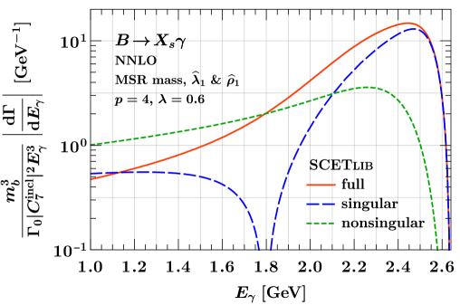
Figure -359: Comparison of the absolute values of the singular, nonsingular, and full contributions to the $B\to X_{s}\gamma$ photon energy spectrum at fixed NNLO in the MSR scheme.

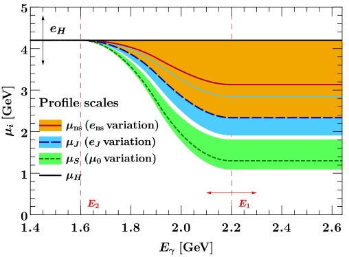
Figure -358: Profile scales used for the hard, jet, soft, and nonsingular scales. The bands show the individual ranges for the jet, soft, and nonsingular scales. The black and red arrows indicate the variations for the parameter $e_{H}$ and the transition point $E_{1}$.

Figure -359 shows the absolute values of the singular and nonsingular contributions as well as the full result at NNLO (i.e. without resummation), which is used to pick the transition points $E_{1}$ and $E_{2}$ between the different parametric regions. For $E_{\gamma}\gtrsim E_{1}=2.2\,\mathrm{GeV}$, the singular contributions clearly dominate, which also corresponds to the nonperturbative region. For $E_{\gamma}\lesssim E_{2}=1.6\,\mathrm{GeV}$, there are large cancellations between the singular and nonsingular contributions. This corresponds to the fixed-order region, where the separation into singular and nonsingular is ill-defined and only their sum is meaningful. Therefore, the resummation of the singular must be turned off to ensure that this cancellation is not spoiled by it and the correct full result is recovered. Since there is little space between $E_{1}$ and $E_{2}$, the transition region in between them effectively coincides with the intermediate shape function OPE region.

To summarize we use the following values for the profile scale parameters [15]:

$$e_{H} =\{1,1/2,2\}\,,\quad \mu_{0} =\max(1,e_{H})\times\{1.3,1.1,1.8\}\,\mathrm{GeV}\,,$$

$$e_{J} =\{0,-1/3,+1/3\}\,,\quad e_{\rm ns} =\{0,-1,+1\}\,,$$

$$E_{1} =\{2.2,2.1,2.3\}\,\mathrm{GeV}\,,\quad E_{2} =1.6\,\mathrm{GeV}\,.$$ (2.20)

For each parameter, the first value in the set is the central value and the next two are the variations that we will use to assess perturbative uncertainties in section 4. The central values for the profile scales along with their individual variation ranges are illustrated in figure -358. Since the nonsingular contributions are treated at fixed order, a priori there is no canonical scaling to guide the choice of the nonsingular scale $\mu_{\mathrm{ns}}$ beyond the fixed-order region $E_{\gamma}\geq E_{2}$. In practice, it is picked as the geometric mean of the hard and central jet scales to account for the fact that the nonsingular terms have some sensitivity to scales below $\widehat{m}_{b}$, and this choice is varied up to the hard and down to the central jet scales as shown in figure -358.

Note that the individual scales are not independent of each other but are parametrized in such a way that their relative hierarchies are preserved upon varying the profile parameters. For example, they all depend on $\mu_{H}$, such that varying $\mu_{H}$ up and down (by varying $e_{H}$) simultaneously moves the other scales up and down accordingly. In particular all scales always merge into a common value for $E_{\gamma}\leq E_{2}$ to properly turn off the resummation. Similarly, $\mu_{J}$ and $\mu_{\mathrm{ns}}$ depend on $\mu_{S}$, such that varying $\mu_{0}$ not only varies $\mu_{S}$ but also moves $\mu_{J}$ and $\mu_{\mathrm{ns}}$ up and down accordingly to preserve the hierarchy between them. The variations for $\mu_{J}$ and $\mu_{\mathrm{ns}}$ parametrized by $e_{J}$ and $e_{\mathrm{ns}}$ correspond to small deviations from the default hierarchy. This also means that the $\mu_{0}$, $e_{J}$, and $e_{\mathrm{ns}}$ variations smoothly turn off between $E_{1}$ and $E_{2}$ like the resummation itself, such that below $E_{2}$ only the overall $\mu_{H}$ variation remains corresponding to the usual fixed-order scale variation.

2.5 Shape function

The leading-power factorization theorem for $B\to X_{s}\gamma$ in eq. (2.2) separates all soft dynamics into the soft function

$$S(\omega,\mu)\equiv\langle B|\bar{b}_{v}\delta(iD_{+}-\delta+\omega)b_{v}|B\rangle\,,$$ (2.21)

where $b_{v}$ is the HQET $b$-quark field, $\left|B\right\rangle$ is the full QCD $B$-meson state, and $\delta=m_{B}-m_{b}^{\rm pole}$. This definition of $S(\omega,\mu)$ is such that it has support for $\omega\geq 0$ [32]. The soft function contains both perturbative soft radiation as well as the nonperturbative Fermi motion of the $b$ quark inside the $B$ meson. Following ref. [32], we further factorize it as

$$S(\omega,\mu)=\int\!\mathrm{d}k\,\widehat{C}_{0}(\omega-k,\mu)\,\mathcal{F}(k)\,,$$ (2.22)

where the partonic soft function $\widehat{C}_{0}$ can be calculated in perturbation theory, while the shape function $\mathcal{F}(k)$ is a nonperturbative object. It has support for $k\geq 0$ and peaks around $k\sim\Lambda_{\rm QCD}$.

In the tail region where $\omega\gg\Lambda_{\rm QCD}$, the right-hand side of eq. (2.22) can be expanded in powers of $\Lambda_{\rm QCD}/\omega$,

$$S(\omega,\mu)=\sum_{n=0}^{\infty}\frac{(-1)^{n}}{n!}\frac{\mathrm{d}^{n}\widehat{C}_{0}(\omega,\mu)}{\mathrm{d}\omega^{n}}M_{n}\,,$$ (2.23)

where $M_{n}\sim\Lambda_{\rm QCD}^{n}$ are the moments

$$M_{n}\equiv\int\!\mathrm{d}k\,k^{n}\mathcal{F}(k)\,.$$ (2.24)

Hence, in the tail region the leading nonperturbative corrections are encoded in the first few nonperturbative moments of $\mathcal{F}(k)$, and its moment expansion recovers the local-OPE description of the spectrum. On the other hand, in the peak region where $\omega\sim\Lambda_{\rm QCD}$, the full function $\mathcal{F}(k)$ is needed.

As discussed in ref. [32], an important feature of the factorization in eq. (2.22) is that it provides a common description of the nonperturbative effects across these different kinematic regions, incorporating all available perturbative information in the limit $\omega\gg\Lambda_{\rm QCD}$ without having to explicitly carry out an expansion in $\Lambda_{\rm QCD}/\omega$, whose precise region of validity would be unclear. That is, all perturbative corrections to moments of $S(\omega,\mu)$ are encoded in the perturbative function $\widehat{C}_{0}(\omega)$, while the shape function $\mathcal{F}(k)$ is a genuinely nonperturbative function that is formally independent of the perturbative order and can be extracted from experimental data.

The first few moments of $\mathcal{F}(k)$ are given in terms of $B$-meson matrix elements of local HQET operators,

$$M_{0} =1\,,$$

$$M_{1} =m_{B}-\widehat{m}_{b}+\dotsb\,,$$

$$M_{2} =(m_{B}-\widehat{m}_{b})^{2}-\frac{\widehat{\lambda}_{1}}{3}+\dotsb\,,$$

$$M_{3} =(m_{B}-\widehat{m}_{b})^{3}-\widehat{\lambda}_{1}(m_{B}-\widehat{m}_{b})+\frac{\widehat{\rho}_{1}}{3}+\dotsb\,,$$ (2.25)

The hadronic parameters $\widehat{\lambda}_{1}$ and $\widehat{\rho}_{1}$ are matrix elements of local HQET operators defined in a short-distance scheme as discussed in section 3.3. The ellipses denote terms that suppressed by relative powers of $\Lambda_{\rm QCD}/\widehat{m}_{b}$ arising from subleading shape functions that are typically absorbed into $\mathcal{F}(k)$ [15], but which are not relevant for our purposes here.

A general method for parametrizing $\mathcal{F}(k)$ via a systematic expansion around a given base model has been developed in ref. [32], which was used in ref. [15] to fit $\mathcal{F}(k)$ from data. Since our primary interest in this paper are the perturbative corrections, the precise form of $\mathcal{F}(k)$ is not relevant here. We only need a reasonably realistic model for it in order to illustrate our results numerically. For this purpose, we take the exponential base model used in refs. [32, 15], given by

$$\mathcal{F}(k)=\frac{1}{\lambda}Y\Bigl{(}\frac{k}{\lambda}\Bigr{)}\qquad\text{with}\qquad Y(x)=\frac{(p+1)^{p+1}x^{p}}{p!}e^{-(p+1)x}\,.$$ (2.26)

Its normalization and first moment are

$$M_{0}=\int\limits_{0}^{\infty}\!\mathrm{d}k\,\mathcal{F}(k)=1\,,\qquad M_{1}=\int\limits_{0}^{\infty}\!\mathrm{d}k\,k\,\mathcal{F}(k)=\lambda\,.$$ (2.27)

By picking $\lambda\approx m_{B}-\widehat{m}_{b}\approx 0.6\,\mathrm{GeV}$ this base model already provides a good fit of the experimental measurements [15].

Note that evaluating the NⁿLO soft function in a short-distance scheme involves taking $n$ derivatives of $\mathcal{F}(k)$. Therefore, at N³LL^′, which needs the N³LO soft function, and assuming integer $p$, we require $p\geq 4$ to ensure that the soft function vanishes for $\omega\to 0$, which in turn is required for the $E_{\gamma}$ spectrum to vanish at the kinematic endpoint $E_{\gamma}\to m_{B}/2$.

3 Short-distance schemes

A major challenge in $B$ physics is to parametrize nonperturbative effects in such a way that their extraction from experimental measurements is stable with (and ideally independent of) the perturbative order. Achieving this stability is not trivial due to infrared sensitivity of the involved perturbative series and the resulting ambiguity in the asymptotic series of perturbative QCD, which is known as the renormalon problem. The renormalon problem manifests itself in practice as poor or no convergence of the perturbative series even at low orders. Since physical (measurable) quantities are independent of the perturbative order, the large perturbative corrections at each order are compensated by corresponding large changes in some associated nonperturbative parameter. In other words, the renormalon ambiguity in the perturbative series is compensated order by order by an equal and opposite renormalon ambiguity in the nonperturbative parameter.

Conceptually, to resolve this issue, the renormalon must be identified and subtracted from both the perturbative quantity ($C$) and the associated parameter ($p$), such that both become renormalon free and perturbatively stable. To give a simple toy example,

$$C-p=(C-\delta p)-(p-\delta p)\equiv\widehat{C}-\widehat{p}\,.$$ (3.1)

On the left-hand side, the renormalon only cancels between $C$ and $p$. On the right-hand side, the so-called residual term $\delta p$ is a perturbative series in $\alpha_{s}$ that contains the renormalon. Its specific choice defines a specific so-called short-distance scheme. The renormalon then cancels within each of the parenthesis defining the short-distance $\widehat{C}$ and $\widehat{p}$, which are now separately free of the renormalon.

3.1 Soft function

In reality, the structure is of course more complicated than the above simple toy example. In our case, the leading-power perturbative series that suffers from renormalon ambiguities is that of the partonic soft function $C_{0}(\omega,\mu)$, whose renormalons are cancelled by the nonperturbative object $\mathcal{F}(k)$. Its leading renormalon ambiguity of $\mathcal{O}(\Lambda_{\rm QCD})$ is due to the pole mass definition of the $b$ quark, $m_{b}^{\rm pole}$, which explicitly enters in the definition of the soft function $S(\omega,\mu)$ in eq. (2.21) and henceforth shows up in all the moments of $\mathcal{F}(k)$. (At subleading power, also the jet and hard functions involve the pole-mass renormalon, which we come back to in section 3.4.) Furthermore, the hadronic parameter $\lambda_{1}$, which first appears in the second moment of $\mathcal{F}(k)$, has a subleading $\mathcal{O}(\Lambda_{\rm QCD}^{2})$ renormalon ambiguity [41]. Similarly, we expect the hadronic parameter $\rho_{1}$, which first appears in the third moment, to have an $\mathcal{O}(\Lambda_{\rm QCD}^{3})$ renormalon.

We write the parameters in a generic short-distance scheme as

$$\widehat{m}_{b}=m_{b}^{\rm pole}-\delta m_{b}\,,\qquad\widehat{\lambda}_{1}=\lambda_{1}-\delta\lambda_{1}\,,\qquad\widehat{\rho}_{1}=\rho_{1}-\delta\rho_{1}\,.$$ (3.2)

The residual terms $\delta m_{b}$, $\delta\lambda_{1}$, and $\delta\rho_{1}$ are defined to cancel the renormalon in their respective parameter such that the short-distance parameters on the left-hand side are renormalon free. The original HQET parameters $\lambda_{1}$ and $\rho_{1}$ are defined in dimensional regularization as [42]

$$\lambda_{1}=\left\langle B\right|\bar{b}_{v}(iD)^{2}b_{v}\left|B\right\rangle\,,\qquad\rho_{1}=\left\langle B\right|\bar{b}_{v}(iD_{\mu})(v\cdot iD)(iD^{\mu})b_{v}\left|B\right\rangle\,.$$ (3.3)

The construction of the short-distance partonic soft function $\widehat{C}_{0}(\omega,\mu)$ with the appropriate renormalon subtractions is derived in detail in ref. [32]. Up to N³LO, we have

$$\widehat{C}_{0}(\omega,\mu) =\biggl{[}1-\frac{\delta\lambda_{1}}{6}\frac{\mathrm{d}^{2}}{\mathrm{d}\omega^{2}}-\frac{\delta\rho_{1}}{18}\frac{\mathrm{d}^{3}}{\mathrm{d}\omega^{3}}+\cdots\biggr{]}e^{\delta m_{b}\frac{\mathrm{d}}{\mathrm{d}\omega}}C_{0}(\omega,\mu)$$

$$=\biggl{[}1+\delta m_{b}\frac{\mathrm{d}}{\mathrm{d}\omega}+\frac{1}{2}\biggl{(}\delta m_{b}^{2}-\frac{\delta\lambda_{1}}{3}\biggr{)}\frac{\mathrm{d}^{2}}{\mathrm{d}\omega^{2}}$$

$$\quad+\frac{1}{6}\biggl{(}\delta m_{b}^{3}-\delta m_{b}\delta\lambda_{1}-\frac{\delta\rho_{1}}{3}\biggr{)}\frac{\mathrm{d}^{3}}{\mathrm{d}\omega^{3}}+\cdots\biggr{]}C_{0}(\omega,\mu)\,,$$ (3.4)

where the original pole-scheme $C_{0}(\omega,\mu)$ is defined and given in appendix A.4. Importantly, for the renormalons to cancel on the right-hand side, it must always be fully expanded to a given fixed order in $\alpha_{s}$, including the $\delta m_{b}$, $\delta\lambda_{1}$, $\delta\rho_{1}$ and their products with each other and with $C_{0}$. With these subtractions both $\widehat{C}_{0}(\omega,\mu)$ and $\mathcal{F}(k)$ become renormalon free, up to yet higher-order renormalons. In particular, the moments of $\mathcal{F}(k)$ are then given by the short-distance parameters $\widehat{m}_{b}$, $\widehat{\lambda}_{1}$, $\widehat{\rho}_{1}$, as shown in eq. (2.5). [Note that $\mathcal{F}(k)\equiv\widehat{\mathcal{F}}(k)$ in eq. (2.22) is already the short-distance parameter.] To evaluate the convolution integral $\widehat{C}_{0}\otimes\mathcal{F}$, we use integration by parts to move all the derivatives in eq. (3.1) to act on $\mathcal{F}$ [32]. The renormalon subtractions significantly improve the perturbative convergence of the soft function compared to the pole scheme, which we demonstrate numerically in section 5.3.

In general, the residual terms are scale dependent, leading to a similar scale dependence of the short-distance parameter, which we suppress for simplicity in our generic notation. The scale dependence can be explicit, as e.g. for the $\overline{\text{MS}}$ mass, in which case it is usually governed by an associated RGE. It can also be only internal, as e.g. for the 1$S$ mass or the MSR mass, in which case $\delta m_{b}$ (and also $\widehat{m}_{b}$) is formally scale independent (with only the usual scale dependence from truncating the perturbative series that is cancelled by higher orders). In either case, the residual terms must be expanded at the same scale $\mu$, i.e., in terms of the same $\alpha_{s}(\mu)$, that is used for the perturbative series whose renormalon is supposed to be subtracted to ensure that the renormalon actually cancels. In our case this is the soft scale $\mu_{S}$ at which we evaluate the fixed-order boundary condition $\widehat{C}_{0}(\omega,\mu_{S})$ in the factorization theorem in eq. (2.2).

In this context, the power counting of the HQET Lagrangian provides a powerful constraint on the generic size of the residual mass term $\delta m_{b}$,

$$\mathcal{L}_{\rm HQET}=\bar{b}_{v}\,(iv\cdot D-\delta m_{b})\,{b}_{v}\,.$$ (3.5)

A suitable short-distance scheme for the bottom-quark mass should respect the power counting of residual soft momentum $\delta m_{b}\sim\alpha_{s}\,v\cdot D\sim\alpha_{s}\,k\sim\alpha_{s}\Lambda_{\rm QCD}$ [43]. Note that the perturbative series for $\delta m_{b}$ starts at NLO and therefore scales like $\alpha_{s}$. As stated in the previous section, in $B\to X_{s}\gamma$ the residual momentum of the bottom quark in the $B$ meson scales like $k\sim m_{B}-2E_{\gamma}$, which in the peak region scales like $\Lambda_{\rm QCD}$. Thus, in the peak region one expects that a low-scale mass scheme, such as the 1$S$ scheme [29, 30, 31] or the MSR scheme [33] with $R\sim\Lambda_{\rm QCD}$, are applicable. In the context of $B\to X_{s}\gamma$, the 1$S$ mass scheme has been extensively discussed in ref. [32], and we remind the reader of the main features of the MSR scheme in the following section.

3.2 MSR mass scheme

The MSR mass scheme is a short-distance mass scheme designed to subtract the pole-mass renormalon by introducing an infrared cutoff scale $R$ as follows,

$$\delta m_{b}(R)\equiv m_{b}^{\rm pole}-m_{b}^{\rm MSR}(R)=R\sum_{n=1}^{\infty}a_{n}^{\rm MSR}\Bigl{[}\frac{\alpha_{s}(R)}{4\pi}\Bigr{]}^{n}\,,$$ (3.6)

where $a_{n}^{\rm MSR}$ coefficients are determined from matching the MSR mass scheme onto the $\rm\overline{MS}$ mass scheme at $\overline{m}_{b}(\overline{m}_{b})$. The infrared scale $R$ controls the size of self-energy contributions which are absorbed into the mass definition [33, 44]. In our analysis we use the so-called “natural” MSR mass definition, where the series coefficients $a_{n}^{\rm MSR}=a_{n}^{\overline{\text{MS}}}(n_{l},n_{h}=0)$ , see ref. [45] for more details.

The MSR mass is a natural extension of the $\overline{\text{MS}}$ mass for $R\leq\overline{m}_{b}(\overline{m}_{b})$, which interpolates between all short-distance schemes with residual power counting $\delta m_{b}(R)\sim R\,\alpha_{s}$. In the limit where $m_{b}^{\rm MSR}(m^{\rm MSR}_{b})\to\overline{m}_{b}(\overline{m}_{b})$ one approaches the $\overline{\text{MS}}$ mass, whereas in the opposite limit, $R\to 0$ , the MSR mass formally approaches the pole mass. In practice, when taking this limit one encounters the Landau pole of the coupling constant. This issue is deeply related to the pole mass renormalon and cannot be addressed unambiguously.

Values of the MSR mass at different $R$ scales are related by the so-called $R$-evolution equation [33], whose solution resums logarithms $\ln(R_{1}/R_{0})$ in the perturbative correction between $m_{b}^{\rm MSR}(R_{1})$ and $m_{b}^{\rm MSR}(R_{0})$. The $R$ evolution can be used to obtain the MSR mass value at a low $R$ from the $\overline{\text{MS}}$ mass and vice versa.

In contrast to the 1$S$ scheme, the infrared scale $R$ of the MSR scheme is an external parameter. We exploit this feature and pick $R=1\,\mathrm{GeV}$ to be of the same order as the soft scale in the peak region. In section 5.3 we demonstrate that this ensures a proper cancellation of the renormalon in the soft function. In principle, it is possible to pick a different value for the $R$ scale in different regions of the spectrum by introducing a profile function $R(E_{\gamma})$ [46], as long as the $R$ evolution is consistently used to relate the shape functions at different $R$ scales. This can be used to enforce $R\sim\mu_{S}$ over the whole spectrum and to eliminate logarithms $\ln(\mu_{S}/R)$ in the series of $\delta m_{b}(R)$. Ref. [40] implements this $R$-evolution setup for an analogous soft function for the thrust distribution in jet production. In our case the use of $R$ evolution does not lead to a significant improvement in convergence, so for simplicity in our numerical analysis we use a fixed value of $R$.

3.3 Short-distance schemes for $\lambda_{1}$ and $\rho_{1}$

To express the $B$-meson matrix elements $\lambda_{1}$ and $\rho_{1}$ in a short-distance scheme, we use analogous schemes to the “invisible” scheme for $\lambda_{1}$ [32], where $\delta\lambda_{1}\propto\alpha_{s}^{2}$. The reason for this $\alpha_{s}^{2}$ scaling in the invisible scheme compared to the kinetic scheme [47, 48], where $\delta\lambda_{1}\propto\alpha_{s}$, is that in the invisible scheme one employs Lorentz-invariant UV regulators for regularizing the kinetic energy operator [41, 49], while in the kinetic scheme the regulator is not Lorentz-invariant. Indeed it has been shown in ref. [32] that using the kinetic scheme for $\lambda_{1}$ leads to an over-subtraction of the $u=1$ renormalon in the soft function. It is worth to note here that there is no analogous study for the $u=3/2$ renormalon present in $\rho_{1}$. Following these features of the invisible scheme for $\lambda_{1}$, we write

$$\delta\lambda_{1}(R_{\lambda},\mu) =R_{\lambda}^{2}\,\frac{\alpha_{s}^{2}(\mu)}{\pi^{2}}\biggl{[}\delta\lambda_{1}^{(2)}+\frac{\alpha_{s}(\mu)}{\pi}\Bigl{(}\delta\lambda_{1}^{(3)}+\delta\lambda_{1}^{(2)}\,\beta_{0}\,\ln\frac{\mu}{R_{\lambda}}\Bigr{)}\biggr{]}+\mathcal{O}(\alpha_{s}^{4})\,,$$

$$\delta\rho_{1}(R_{\rho},\mu) =R_{\rho}^{3}\,\frac{\alpha_{s}^{3}(\mu)}{\pi^{3}}\,\delta\rho_{1}^{(3)}+\mathcal{O}(\alpha_{s}^{4})\,,$$ (3.7)

where we set $R_{\lambda}=R_{\rho}=1\,\mathrm{GeV}$ by default. Note that $\lambda_{1}$ and $\rho_{1}$ appear in the second and third moments of the shape function and contain an $\mathcal{O}(\Lambda_{\rm QCD}^{2})$ and $\mathcal{O}(\Lambda_{\rm QCD}^{3})$ renormalon ambiguities, respectively. Therefore by dimensional analysis they must scale like $\delta\lambda_{1}\propto R_{\lambda}^{2}$ and $\delta\rho_{1}\propto R_{\rho}^{3}$. Furthermore, we take $\delta\rho_{1}\propto\alpha_{s}^{3}$ to impose a plausible “invisibility” of our scheme choice and to avoid diluting the lower-order corrections arising from $\delta m_{b}$ and $\delta\lambda_{1}$. For $\delta\lambda_{1}^{(2)}$ we use the value given in ref. [32] for the invisible scheme, $\delta\lambda_{1}^{(2)}=\pi^{2}/3-1$. Values of $\delta\lambda_{1}^{(3)}$ and $\delta\rho_{1}^{(3)}$ are not available so far.

Usually, one defines a short-distance scheme to all orders by exploiting the perturbative series of some physical and thus renormalon-free quantity. However, this is not strictly necessary, since after all the main goal of the renormalon subtractions is to obtain a stable perturbative result. Thus, here we take a pragmatic approach and simply define our “invisible” scheme for $\widehat{\lambda}_{1}$ and $\widehat{\rho}_{1}$ at $\mathcal{O}(\alpha_{s}^{3})$ by choosing numerical values for $\delta\lambda_{1}^{(3)}$ and $\delta\rho_{1}^{(3)}$ such that the resulting soft function at different perturbative orders manifests good convergence, i.e. that the size of scale variations reduces when including higher-order corrections, that the resulting uncertainty bands at different orders have reasonable overlaps, that the peak position for the soft function remains stable, and finally that it remains positive at small $k$ and approaches zero with similar slopes at different orders. Following this procedure, we find a satisfactory convergence for the soft function, see figure -349, by taking

$$\delta\lambda_{1}^{(3)}=16\,,\qquad\delta\rho_{1}^{(3)}=-3\,.$$ (3.8)

In principle, we could also consider the perturbative convergence of the final spectrum. However, since it also receives contributions from the jet and hard functions, the dependence on the soft function is washed out in the spectrum. Therefore, we use the convergence of the soft function to define the short-distance scheme. This is also the most natural, since the soft function is the object containing the renormalons to be subtracted. This is somewhat similar to the “shape-function” scheme in ref. [50], where the second and third moments of the perturbative shape function with some, largely arbitrary, hard cutoff is used to define the short-distance parameters. (Similarly, the short-distance $b$-quark mass is defined based on the first moment.) The disadvantage of that approach is that it yields $\delta\lambda,\delta\rho_{1}\sim\alpha_{s}$, which leads to massive oversubtraction similar to the kinetic scheme.

3.4 Subleading $\delta m_{b}$ corrections

As discussed in section 3.1, the leading renormalon at leading power comes from the $b$-quark mass that enters via the argument of the soft function. In addition to the soft function, the $b$-quark mass also enters in the hard and jet functions through the SCET label momentum $p^{-}\sim m_{b}$. By default, label momentum conservation sets $p^{-}=m_{b}^{\rm pole}$. Formally, choosing a different label $p^{-}=\widehat{m}_{b}$ amounts to a power-suppressed effect. For this reason, in ref. [15] the resulting corrections from changing to the $\widehat{m}_{b}$ scheme could effectively be absorbed into the nonsingular corrections. As we will see, at N³LL^′ this is no longer viable, so instead we will explicitly switch both hard and jet functions to a short-distance mass scheme.

To derive the scheme change, we consider the partonic function $W(k)$ appearing in eq. (2.3), which can be either the singular, the nonsingular, or the full contribution. It has mass dimension $-1$ and depends on two dimensionful quantities, $k$ and $m_{b}$. Therefore, by dimensional analysis it must have the form

$$W(k)=\frac{1}{m_{b}}w\Bigl{[}\frac{k}{m_{b}},\alpha_{s}(\mu),\ln\frac{\mu}{m_{b}}\Bigr{]}=\frac{1}{m_{b}}w\Bigl{[}\frac{k}{m_{b}},\alpha_{s}(m_{b})\Bigr{]}\,,$$ (3.9)

where all dependence on $m_{b}$ is made explicit on the right-hand side and $w(x,\alpha_{s},L)$ is a scaleless function of its arguments. Since $W(k)$ is defined to be $\mu$ independent, the $\mu$ dependence on the right-hand is only the internal $\mu$ dependence from $\alpha_{s}(\mu)$ which cancels order by order. Therefore, we can pick $\mu=m_{b}$, which eliminates all logarithms and allows us to track the associated $m_{b}$ dependence via the dependence on $\alpha_{s}(m_{b})$. After switching the scheme, we can easily reintroduce the $\mu$ dependence by reexpanding $\alpha_{s}(m_{b})$ in terms of $\alpha_{s}(\mu)$.

The partonic rate in the pole scheme is given by eq. (3.9) evaluated at $k=m_{b}^{\rm pole}-2E_{\gamma}$ and $m_{b}=m_{b}^{\rm pole}$. To switch to a short-distance scheme, we thus have to replace $k\to k+\delta m_{b}$ and $m_{b}\to m_{b}^{\rm pole}=\widehat{m}_{b}+\delta m_{b}$ in eq. (3.9) and expand in $\delta m_{b}$. This gives

$$\widehat{m}_{b}W(\widehat{m}_{b}x) =\frac{1}{1+\delta m_{b}/\widehat{m}_{b}}w\Bigl{(}\frac{x+\delta m_{b}/\widehat{m}_{b}}{1+\delta m_{b}/\widehat{m}_{b}},\alpha_{s}(\widehat{m}_{b}+\delta m_{b})\Bigr{)}$$

$$=\biggl{\{}1+\frac{\delta m_{b}}{\widehat{m}_{b}}\frac{\mathrm{d}}{\mathrm{d}x}(1-x)+\frac{1}{2}\frac{\delta m_{b}^{2}}{\widehat{m}_{b}^{2}}\frac{\mathrm{d}^{2}}{\mathrm{d}x^{2}}(1-x)^{2}$$

$$\quad+\frac{1}{3!}\frac{\delta m_{b}^{3}}{\widehat{m}_{b}^{3}}\frac{\mathrm{d}^{3}}{\mathrm{d}x^{3}}(1-x)^{3}+\frac{\delta m_{b}}{\widehat{m}_{b}}\beta[\alpha_{s}(\widehat{m}_{b})]\frac{\mathrm{d}}{\mathrm{d}\alpha_{s}}+\mathcal{O}(\alpha_{s}^{4})\biggr{\}}w[x,\alpha_{s}(\widehat{m}_{b})]\,,$$ (3.10)

where for convenience we multiplied by $\widehat{m}_{b}$ and switched variables, $k=\widehat{m}_{b}x$, such that $\widehat{m}_{b}W(\widehat{m}_{b}x)$ is a dimensionless function of $x$. In the second step, we expanded in $\delta m_{b}$ keeping only terms that contribute up to $\mathcal{O}(\alpha_{s}^{3})$, recalling that $\delta m_{b}\sim\mathcal{O}(\alpha_{s})$ and $\beta(\alpha_{s})\sim\alpha_{s}^{2}$. The derivatives act on everything to their right.

Substituting the explicit $\alpha_{s}$ expansions for $\delta m_{b}/\widehat{m}_{b}$, $\beta(\alpha_{s})$, and $w(x,\alpha_{s})$, it is straightforward to derive the correction terms $\Delta w_{77}^{\mathrm{s}(n)}$ and $\Delta w_{77}^{\mathrm{ns}(n)}$ appearing in eqs. (2.2) and (2.3). Writing the $\alpha_{s}$ expansion of $\delta m_{b}/\widehat{m}_{b}$ as

$$\frac{\delta m_{b}}{\widehat{m}_{b}}=\frac{\alpha_{s}(\mu)}{4\pi}\,\delta_{m}^{(1)}(\mu)+\Bigl{[}\frac{\alpha_{s}(\mu)}{4\pi}\Bigr{]}^{2}\delta_{m}^{(2)}(\mu)+\Bigl{[}\frac{\alpha_{s}(\mu)}{4\pi}\Bigr{]}^{3}\delta_{m}^{(3)}(\mu)+\mathcal{O}(\alpha_{s}^{4})\,,$$ (3.11)

we find for the singular

$$\Delta w_{77}^{\mathrm{s}(1)}(\mu,x) =\frac{1}{4}\delta_{m}^{(1)}(\mu)\frac{\mathrm{d}}{\mathrm{d}x}w_{77}^{\mathrm{s}(0)}(x)\,,$$

$$\Delta w_{77}^{\mathrm{s}(2)}(\mu,x) =\frac{1}{16}\biggl{\{}\delta_{m}^{(2)}(\mu)\frac{\mathrm{d}}{\mathrm{d}x}+\frac{1}{2}\bigl{[}\delta_{m}^{(1)}(\mu)\bigr{]}^{2}\frac{\mathrm{d}^{2}}{\mathrm{d}x^{2}}\biggr{\}}w_{77}^{\mathrm{s}(0)}(x)$$

$$\quad+\frac{1}{4}\delta_{m}^{(1)}(\mu)\frac{\mathrm{d}}{\mathrm{d}x}\bigl{[}(1-x)w_{77}^{\mathrm{s}(1)}(x)\bigr{]}\,,$$

$$\Delta w_{77}^{\mathrm{s}(3)}(\mu,x) =\frac{1}{64}\biggl{\{}\delta_{m}^{(3)}(\mu)\frac{\mathrm{d}}{\mathrm{d}x}+\delta_{m}^{(1)}(\mu)\delta_{m}^{(2)}(\mu)\frac{\mathrm{d}^{2}}{\mathrm{d}x^{2}}+\bigl{[}\delta_{m}^{(1)}(\mu)\bigr{]}^{3}\frac{1}{3!}\frac{\mathrm{d}^{3}}{\mathrm{d}x^{3}}\biggr{\}}w_{77}^{\mathrm{s}(0)}(x)$$

$$\quad+\frac{1}{16}\biggl{\{}-2\beta_{0}\delta_{m}^{(1)}(\mu)+\Bigl{[}\delta_{m}^{(2)}(\mu)+2\beta_{0}\delta_{m}^{(1)}(\mu)\ln\frac{\mu}{\widehat{m}_{b}}\Bigr{]}\frac{\mathrm{d}}{\mathrm{d}x}(1-x)$$

$$\qquad\qquad+\frac{1}{2}\bigl{[}\delta_{m}^{(1)}(\mu)\bigr{]}^{2}\frac{\mathrm{d}^{2}}{\mathrm{d}x^{2}}(1-x)^{2}\biggr{\}}w_{77}^{\mathrm{s}(1)}(x)$$

$$\quad+\frac{1}{4}\delta_{m}^{(1)}(\mu)\frac{\mathrm{d}}{\mathrm{d}x}(1-x)w_{77}^{\mathrm{s}(2)}(x)\,,$$ (3.12)

and the nonsingular

$$\frac{\Delta w^{\mathrm{ns}(2)}_{77}(\mu_{\mathrm{ns}},x)}{(1-x)^{3}} =\frac{1}{4}\delta_{m}^{(1)}(\mu_{\mathrm{ns}})\frac{\mathrm{d}}{\mathrm{d}x}\biggl{[}\frac{w_{77}^{\mathrm{ns}(1)}(x)}{(1-x)^{2}}\biggr{]}\,,$$

$$\frac{\Delta w^{\mathrm{ns}(3)}_{77}(\mu_{\mathrm{ns}},x)}{(1-x)^{3}} =\frac{1}{16}\biggl{\{}-2\beta_{0}\delta_{m}^{(1)}(\mu_{\mathrm{ns}})+\Bigl{[}\delta_{m}^{(2)}(\mu_{\mathrm{ns}})+2\beta_{0}\delta_{m}^{(1)}(\mu_{\mathrm{ns}})\ln\frac{\mu_{\mathrm{ns}}}{\widehat{m}_{b}}\Bigr{]}\frac{\mathrm{d}}{\mathrm{d}x}(1-x)$$

$$\qquad\quad+\frac{1}{2}\bigl{[}\delta_{m}^{(1)}(\mu_{\mathrm{ns}})\bigr{]}^{2}\frac{\mathrm{d}^{2}}{\mathrm{d}x^{2}}(1-x)^{2}\biggr{\}}\frac{w_{77}^{\mathrm{ns}(1)}(x)}{(1-x)^{3}}$$

$$\quad+\frac{1}{4}\delta_{m}^{(1)}(\mu_{\mathrm{ns}})\frac{\mathrm{d}}{\mathrm{d}x}\frac{w_{77}^{\mathrm{ns}(2)}(x)}{(1-x)^{2}}\,.$$ (3.13)

As we have seen above, there are three sources of $\delta m_{b}$ corrections:

1. Shifting the argument $k\to k+\delta m_{b}$.

2. Changing to $\widehat{m}_{b}$ in the argument $k/\widehat{m}_{b}$, which yields the rescaling $x\to x/(1+\delta m_{b}/\widehat{m}_{b})$.

3. Changing to $\widehat{m}_{b}$ in the $\mu$ dependence of $\alpha_{s}(\widehat{m}_{b})$.

Considering just the singular contributions and only keeping the first and neglecting the latter two corrections amounts to only keeping the leading-power terms in eq. (3.4),

$$\widehat{m}_{b}W^{\mathrm{s}}(\widehat{m}_{b}x) =\biggl{[}1+\frac{\delta m_{b}}{\widehat{m}_{b}}\frac{\mathrm{d}}{\mathrm{d}x}+\frac{1}{2}\frac{\delta m_{b}^{2}}{\widehat{m}_{b}^{2}}\frac{\mathrm{d}^{2}}{\mathrm{d}x^{2}}+\frac{1}{3!}\frac{\delta m_{b}^{3}}{\widehat{m}_{b}^{3}}\frac{\mathrm{d}^{3}}{\mathrm{d}x^{3}}\biggr{]}w^{\mathrm{s}}[x,\alpha_{s}(\widehat{m}_{b})]\,.$$ (3.14)

The relevant formal power counting here is $\delta m_{b}/\widehat{m}_{b}\sim\lambda\ll 1$, $\mathrm{d}/\mathrm{d}x\sim 1/x\sim\lambda^{-1}$, so all terms on the right-hand side are leading power. These terms are exactly reproduced by the factorized result at fixed order by changing the soft function to the $\widehat{m}_{b}$ scheme, which involves the analogous shift of its argument. In the numerical implementation, the derivatives $\mathrm{d}/\mathrm{d}(\widehat{m}_{b}x)=\mathrm{d}/\mathrm{d}k$ are moved via integration by parts to act on the shape function $\mathcal{F}(k)$ so they count as $1/\Lambda_{\rm QCD}$. Since $\delta m_{b}\sim\Lambda_{\rm QCD}$, we see again that all terms in eq. (3.14) are leading power, counting as $(\delta m_{b}\,\mathrm{d}/\mathrm{d}k)^{n}\sim 1$.

All terms $\sim x^{n}w^{\mathrm{s}}(x,\alpha_{s})$ are thus induced by the second source. By moving the derivatives to act onto the shape function, we see that they are explicitly power-suppressed by $x$ and hence nonsingular. For this reason, they could be included as part of the nonsingular correction terms $\Delta w_{77}^{\mathrm{ns}}$, as was done in ref. [15]. In the singular contributions, the $k/m_{b}$ dependence only appears in logarithms which are factorized into the soft, jet, and hard functions, where $m_{b}$ corresponds to the large $p^{-}$ label momentum, which only appears in the hard and jet functions, while the soft function only depends on the small momentum $k$. Therefore, the associated correction terms can be reproduced by the leading-power factorized result by changing the $m_{b}$ dependence in the hard and jet functions to the short-distance $\widehat{m}_{b}$.

Finally, the third source produces the last term in eq. (3.4),

$$\frac{\delta m_{b}}{\widehat{m}_{b}}\beta(\alpha_{s})\frac{\mathrm{d}}{\mathrm{d}\alpha_{s}}[w(x,\alpha_{s}(\widehat{m}_{b})]=-\frac{\alpha_{s}^{3}C_{F}}{8\pi^{3}}\,\delta_{m}^{(1)}\,\beta_{0}\,w_{77}^{\mathrm{s}(1)}(x)+\mathcal{O}(\alpha_{s}^{4})\,.$$ (3.15)

Since it starts at $\mathcal{O}(\alpha_{s}^{3})$ it first appears at N³LL^′. Formally, this term is also subleading power, because $\delta m_{b}/\widehat{m}_{b}\sim\lambda$. However, since there is no explicit kinematic suppression by $x$, the $x$ dependence itself is still singular $\sim 1/x$, involving $\delta(x)$ and logarithmic plus distributions. Hence, this term cannot simply be absorbed into the nonsingular contributions but must be properly accounted for in the resummed singular contribution. The $\widehat{m}_{b}$ dependence in the corresponding fixed-order $\ln(\mu/\widehat{m}_{b})$ also corresponds to the $p^{-}$ label momentum. Therefore, to account for the distributional structure of this contribution and to resum it, we consistently switch the hard and jet functions to the short-distance mass $\widehat{m}_{b}$. The details of this procedure are discussed in the following two subsections.

3.5 Hard function

The hard function in a short-distance scheme is obtained by writing the $b$-quark mass in the pole-scheme hard function in eq. (A.5) in terms of a short-distance mass and reexpanding the result strictly in powers of $\alpha_{s}(\mu)$. At $\rm N^{3}LO$ we obtain

$$\widehat{h}_{s}(\widehat{m}_{b},\mu)=h_{s}(\widehat{m}_{b},\mu)-\sum_{n=2}^{\infty}\sum_{m=0}^{2n-3}\Delta H_{m}^{(n)}(\mu)\biggl{[}\frac{\alpha_{s}(\mu)}{4\pi}\biggr{]}^{n}\ln^{m}\!\frac{\mu}{\widehat{m}_{b}}\,,$$ (3.16)

where the coefficients $\Delta H_{m}^{(n)}$ are given by

$$\Delta H_{0}^{(2)}(\mu) =\delta_{m}^{(1)}(\mu)H_{1}^{(1)}\,,$$

$$\Delta H_{1}^{(2)}(\mu) =2\delta_{m}^{(1)}(\mu)H_{2}^{(1)}\,,$$

$$\Delta H_{0}^{(3)}(\mu) =\delta_{m}^{(2)}(\mu)H_{1}^{(1)}+\delta_{m}^{(1)}(\mu)H_{1}^{(2)}-\frac{1}{2}\bigl{(}\delta_{m}^{(1)}(\mu)\bigr{)}^{2}\Bigl{(}H_{1}^{(1)}+2H_{2}^{(1)}\Bigr{)}\,,$$

$$\Delta H_{1}^{(3)}(\mu) =2\delta_{m}^{(2)}(\mu)H_{2}^{(1)}+2\delta_{m}^{(1)}(\mu)H_{2}^{(2)}-\bigl{(}\delta_{m}^{(1)}(\mu)\bigr{)}^{2}H_{2}^{(1)}\,,$$

$$\Delta H_{2}^{(3)}(\mu) =3\delta_{m}^{(1)}(\mu)H_{3}^{(2)}\,,$$

$$\Delta H_{3}^{(3)}(\mu) =4\delta_{m}^{(1)}(\mu)H_{4}^{(2)}\,.$$ (3.17)

Here $H_{m}^{(n)}$ are the coefficients of the pole-scheme hard function defined in eq. (A.5), and $\delta_{m}^{(n)}(\mu)$ are defined in eq. (3.11).

Similarly, the RGE for the hard function in a short-distance mass scheme is derived by rewriting the pole mass in eq. (A.6) in terms of a short-distance mass,

$$\frac{\mathrm{d}\widehat{h}_{s}(\widehat{m}_{b},\mu)}{\mathrm{d}\ln\mu}=\biggl{\{}\Gamma^{H}[\alpha_{s}(\mu)]\ln\frac{\mu}{\widehat{m}_{b}}+\gamma^{H}[\alpha_{s}(\mu)]+\Delta\gamma^{H}(\mu)\biggr{\}}\widehat{h}_{s}(\widehat{m}_{b},\mu)\,,$$ (3.18)

where

$$\Delta\gamma^{H}(\mu) =\Gamma^{H}[\alpha_{s}(\mu)]\ln\frac{\widehat{m}_{b}}{m_{b}^{\rm pole}}=-\Gamma^{H}[\alpha_{s}(\mu)]\ln\Bigl{(}1+\frac{\delta m_{b}}{\widehat{m}_{b}}\Bigr{)}$$

$$=-\Bigl{[}\frac{\alpha_{s}(\mu)}{4\pi}\Bigr{]}^{2}\Gamma^{H}_{0}\delta_{m}^{(1)}(\mu)$$

$$\quad-\Bigl{[}\frac{\alpha_{s}(\mu)}{4\pi}\Bigr{]}^{3}\biggl{\{}\Gamma^{H}_{1}\delta_{m}^{(1)}(\mu)+\Gamma^{H}_{0}\biggl{[}\delta_{m}^{(2)}(\mu)-\frac{1}{2}(\delta_{m}^{(1)}(\mu))^{2}\biggr{]}\biggr{\}}+\mathcal{O}(\alpha_{s}^{4})\,,$$ (3.19)

and the hard cusp anomalous dimension coefficients $\Gamma_{n}^{H}=-2\Gamma_{n}$ are defined in eq. (A.1). Note that the reexpansion in eqs. (3.16) and (3.18) must be performed in terms of the same $\alpha_{s}(\mu)$, such that $\widehat{h}_{s}(\widehat{m}_{b},\mu)$ in eq. (3.16) indeed satisfies the RGE in eq. (3.18).

We expect that the renormalon associated with the pole mass cancels in the perturbative series of the hard anomalous dimension. The cusp anomalous dimension is universal and arises in the evolution of many perturbative objects with Sudakov double logarithms that do not involve the $b$-quark mass at all. Therefore, the $\Gamma^{H}$ series cannot know about the pole-mass renormalon, so the cancellation must happen between $\gamma^{H}$ and $\Delta\gamma^{H}$. For this reason, it is important to consistently expand $\Delta\gamma^{H}$ in powers of $\alpha_{s}(\mu)$ to the same order as $\gamma^{H}$.

The all-order solution to the differential equation (3.18) can be written as

$$\widehat{U}_{H}(\widehat{m}_{b},\mu_{H},\mu)=U_{H}(\widehat{m}_{b},\mu_{H},\mu)\times\Delta U_{H}(\mu_{H},\mu)\,,$$ (3.20)

where $U_{H}$ is the usual hard evolution factor given in eq. (A.10), and the correction factor $\Delta U_{H}$ is given by

$$\Delta U_{H}(\mu_{H},\mu)=\exp\biggl{[}\int_{\mu_{H}}^{\mu}\!\mathrm{d}\ln\mu\,\Delta\gamma^{H}(\mu)\biggr{]}\,.$$ (3.21)

Note that in general, the $\mu$ dependence of $\Delta\gamma^{H}(\mu)$ coming from $\delta_{m}^{(n)}(\mu)$ can be more involved than for the usual anomalous dimension, such that the $\mu$ integral may have to be performed numerically. Using the MSR mass and up to N³LL, we can still perform the integral by employing an analytic approximation analogous to the one used for the $K$ and $\eta$ integrals in eq. (A.1). We find up to N³LL

$$\ln\Delta U_{H}(\mu_{H},\mu) =\frac{\alpha_{s}(\mu_{H})}{4\pi}\frac{\Gamma^{H}_{0}}{2\beta_{0}}\delta_{\rm MSR}^{(1)}(r-1)$$

$$\quad+\frac{\alpha_{s}(\mu_{H})}{4\pi}\frac{\Gamma^{H}_{0}}{4\beta_{0}}\biggl{\{}\frac{\alpha_{s}(\mu_{H})}{4\pi}\biggl{[}\left(\delta_{\rm MSR}^{(2)}-\frac{1}{2}(\delta_{\rm MSR}^{(1)})^{2}+2\delta_{\rm MSR}^{(1)}\beta_{0}\ln\frac{\mu_{H}}{R}\right)$$

$$\quad+\delta_{\rm MSR}^{(1)}\left(\frac{\Gamma^{H}_{1}}{\Gamma^{H}_{0}}-\frac{\beta_{1}}{\beta_{0}}\right)\biggr{]}(r^{2}-1)-\delta_{\rm MSR}^{(1)}(r-1)^{2}\biggr{\}}\,,$$ (3.22)

where $r=\alpha_{s}(\mu)/\alpha_{s}(\mu_{H})$ and

$$\delta_{\rm MSR}^{(n)} \equiv\frac{R}{m_{b}^{\rm MSR}(R)}\,a_{n}^{\rm MSR}\,.$$ (3.23)

At NNLL only the first line on the right-hand side of eq. (3.5) is kept.

3.6 Jet function

Similar to the hard function in the previous section, we define the jet function in a short-distance scheme by expressing $m_{b}^{\rm pole}$ in terms of a short-distance mass $\widehat{m}_{b}$. To this end, we start with the jet function in the pole scheme given in eq. (A.11) and set $s=m_{b}^{\rm pole}\,\omega$. Then we write $m_{b}^{\rm pole}$ in terms of $\widehat{m}_{b}$ and reexpand the result strictly in powers of $\alpha_{s}(\mu)$, such that $m_{b}^{\rm pole}J(m_{b}^{\rm pole}\omega,\mu_{J})=\widehat{m}_{b}\widehat{J}(\widehat{m}_{b}\omega,\mu_{J})$ order by order. This yields up to ${\rm N^{3}LO}$

$$\widehat{J}(\widehat{m}_{b}\omega,\mu)=J(\widehat{m}_{b}\omega,\mu)+\sum_{n=2}^{3}\sum_{m=-1}^{2n-4}\Delta J_{m}^{(n)}\biggl{[}\frac{\alpha_{s}(\mu)}{4\pi}\biggr{]}^{n}\frac{1}{\mu^{2}}\mathcal{L}_{m}\Bigl{(}\frac{\widehat{m}_{b}\omega}{\mu^{2}}\Bigr{)}\,.$$ (3.24)

The expansion coefficients $\Delta J_{m}^{(n)}$ read

$$\Delta J_{-1}^{(2)}(\mu) =\delta_{m}^{(1)}(\mu)J_{0}^{(1)}\,,$$

$$\Delta J_{0}^{(2)}(\mu) =\delta_{m}^{(1)}(\mu)J_{1}^{(1)}\,,$$

$$\Delta J_{-1}^{(3)}(\mu) =\delta_{m}^{(2)}(\mu)J_{0}^{(1)}+\delta_{m}^{(1)}(\mu)J_{0}^{(2)}-\frac{1}{2}\bigl{(}\delta_{m}^{(1)}(\mu)\bigr{)}^{2}\Bigl{(}J_{0}^{(1)}-J_{1}^{(1)}\Bigr{)}\,,$$

$$\Delta J_{0}^{(3)}(\mu) =\delta_{m}^{(2)}(\mu)J_{1}^{(1)}+\delta_{m}^{(1)}(\mu)J_{1}^{(2)}-\frac{1}{2}\bigl{(}\delta_{m}^{(1)}(\mu)\bigr{)}^{2}J_{1}^{(1)}\,,$$

$$\Delta J_{1}^{(3)}(\mu) =2\delta_{m}^{(1)}(\mu)J_{2}^{(2)}\,,$$

$$\Delta J_{2}^{(3)}(\mu) =3\delta_{m}^{(1)}(\mu)J_{3}^{(2)}\,,$$ (3.25)

where the $\delta_{m}^{(n)}$ are defined in eq. (3.11) and the $J_{m}^{(n)}$ coefficients are those of the original pole-scheme jet function as defined in eq. (A.11).

4 Perturbative uncertainties

For our predictions we can distinguish perturbative and parametric uncertainties. Parametric uncertainties arise from the uncertainty in input parameters, such as $C_{7}^{\rm incl}$, $|V_{\rm tb}\,V_{ts}^{*}|^{2}$, $m_{b}$, $\mathcal{F}(k)$. These are not considered in the following. We normalize our numerical results by dividing out the overall prefactor $\Gamma_{0}\bigl{|}C_{7}^{\rm incl}\bigr{|}^{2}$, so the associated uncertainties drop out. We also ignore the parametric uncertainties due to the shape function $\mathcal{F}(k)$ and $m_{b}$, which do affect the shape of the spectrum, because we do not compare with experimental $B\to X_{s}\gamma$ measurements, in which case they would be determined by the fit to the data.

Our primary focus is on the perturbative results and their perturbative uncertainties arising from missing higher-order corrections. For these there are various different sources, which fall into two categories:

• Profile scale variations: We identify three sources of perturbative uncertainties that are estimated by a suitable set of variations of the profile scales discussed in section 2.4. The resummation uncertainty $\Delta_{\rm resum}$ is obtained by taking the maximum envelope of all $27$ simultaneous variations of the profile function parameters $e_{H}$, $e_{J}$, $\mu_{0}$, which corresponds to scale variations in the resummed singular contributions, together with corresponding correlated variations in the nonsingular contributions. Note also that despite its name, $\Delta_{\rm resum}$ reduces to the overall fixed-order scale variation in the fixed-order region. The nonsingular uncertainty $\Delta_{\rm ns}$ is determined by varying the $e_{\rm ns}$ parameter, which determines the central value of the nonsingular scale in the resummation regions. The matching uncertainty $\Delta_{\rm match}$ comes from varying the transition point $E_{1}$, which marks the start of the transition region. These three sources are considered independent and are thus added in quadrature,

  $$\Delta_{\rm profile}=\Delta_{\rm resum}\oplus\Delta_{\rm ns}\oplus\Delta_{\rm match}\,.$$ (4.1)

  For notational convenience, we use the symbol $\oplus$ to denote addition in quadrature, $x\oplus y\equiv\sqrt{x^{2}+y^{2}}$.

• Theory nuisance parameter variations: The uncertainties $\Delta_{h_{3}}$ and $\Delta_{c^{\rm ns}}$ are estimated by varying the nuisance parameters $h_{3}$ and $c^{\rm ns}_{k}$, respectively, within the ranges given in sections 2.2 and 2.3, where we abbreviate $\Delta_{c^{\rm ns}}=(\sum_{k=0}^{5}\Delta_{c^{\rm ns}_{k}}^{2})^{1/2}$. Note that by definition the central values of all nuisance parameters are zero.

  The nuisance parameters at N³LL${}^{\prime}+$N³LO$(c_{k})$ are introduced in such a way that the scale dependence cancels at this order, i.e., all terms that are predicted by scale dependence are correctly included. This means that at N³LL${}^{\prime}+$N³LO$(c_{k})$ the profile scale variations estimate the uncertainty due to the missing next order N⁴LL${}^{\prime}+$N⁴LO, while the nuisance parameters capture the uncertainty due to the missing $\mathcal{O}(\alpha_{s}^{3})$ ingredients at N³LL${}^{\prime}+$N³LO$(c_{k})$.

The total perturbative uncertainty is obtained by adding all sources in quadrature,

$$\Delta_{\rm total}=\Delta_{\rm profile}\oplus\Delta_{h_{3}}\oplus\Delta_{c^{\rm ns}}\,.$$ (4.2)

The nuisance parameter uncertainties only contribute at the highest order N³LL${}^{\prime}+$N³LO$(c_{k})$, while at lower orders we simply have $\Delta_{\rm total}=\Delta_{\rm profile}$.

Note that in ref. [15] the perturbative uncertainty was estimated from profile scale variations by taking the maximum envelope of $3^{5}=243$ profile scale variations corresponding to simultaneous variations of the above five profile scale parameters. Here we have refined the estimation procedure by separating conceptually different sources of perturbative uncertainties, which leads to an overall more consistent picture of the resulting uncertainties when including the new highest order at N³LL^′. In part, this becomes possible because we are now able to reexpand the fixed-order hard function against the product of the fixed-order jet and soft functions. We have also checked that the total $\Delta_{\rm profile}$ estimated as described above is comparable in size to what we obtain in our setup by taking the maximum envelope of all $3^{5}=243$ variations excluding a small set of obvious outliers.

5 Results

In this section, we present our numerical results for the photon energy spectrum. All numerical results are implemented and obtained with the SCETlib [51] library.

Our default numerical setup is as follows. The values used for input parameters are summarized in table 1. The spectrum is always divided by the overall normalization factor $\Gamma_{0}\bigl{|}C_{7}^{\rm incl}\bigr{|}^{2}$, so its numerical value is not needed. For the shape-function model in eq. (2.26) we use $\lambda=0.6\,\mathrm{GeV}$ and $p=4$ as the default settings. We illustrate the impact of changing $p$ and $\lambda$ later in this section. We neglect finite-charm-mass corrections and work in QCD with $n_{f}=4$ massless quarks. We always use the 4-loop running of $\alpha_{s}$, which is sufficient for resummation at $\rm N^{3}LL$. We use the MSR scheme for the $b$-quark mass and adopt short-distance schemes for $\lambda_{1}$ and $\rho_{1}$ as discussed in section 3.3. The impact of the short-distance mass scheme is discussed in section 5.3. Throughout this section, the colored bands always show the perturbative uncertainties obtained from profile scale variations $\Delta_{\rm profile}$.

Parameter	Value
$m_{B}$	$5.279\,\mathrm{GeV}$
$\alpha_{s}(\mu=4.7\,\mathrm{GeV})$	$0.2155$
$m_{b}^{\rm MSR}(R=1\,\mathrm{GeV})$	$4.7\,\mathrm{GeV}$
$\lambda$	$0.6\,\mathrm{GeV}$
$p$	$4$

Table 1: Numerical values of required input parameters.

5.1 Main results

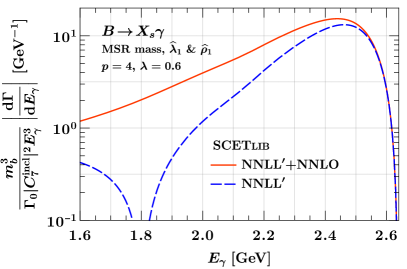
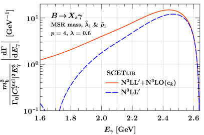
Figure -357: Comparison of the absolute value of resummed contribution to the full $B\to X_{s}\gamma$ photon energy spectrum in the MSR mass scheme. The left panel shows the 2-loop predictions, the right panel shows the 3-loop predictions. The overall factor $\Gamma_{0}\bigl{|}C_{7}^{\rm incl}\bigr{|}^{2}(E_{\gamma}/\widehat{m}_{b})^{3}$ is divided out (see eq. (2.1)).

To begin, in figure -357, we show the contribution of the resummed singular corrections to the full result at NNLL^′ (left panel) and N³LL^′ (right panel). The resummed contribution is indeed dominant across the peak of the spectrum, while it decreases rapidly in the tail and eventually changes sign at $E_{\gamma}\lesssim 1.8\,\mathrm{GeV}$, where the resummation is getting turned off. Here, only the full matched result is meaningful, which remains positive and slowly approaches zero in the far tail.

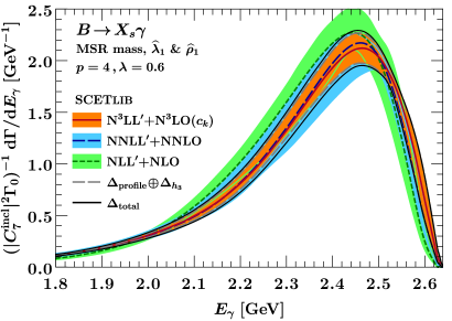
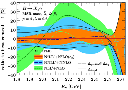
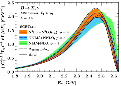
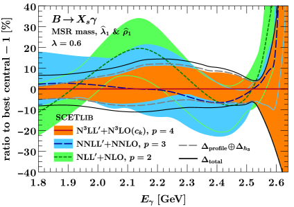
Figure -356: The $B\to X_{s}\gamma$ spectrum at different perturbative orders. The $E_{\gamma}$ spectrum itself is shown on the left, while the relative differences to the highest-order central value are shown on the right. In the top row, we use the same value $p=4$ at each order, while in the bottom row we use successive values at each order. The colored bands show the perturbative uncertainty estimated by just profile scale variations, $\Delta_{\rm profile}$. The dashed gray line includes in addition the uncertainty due to $h_{3}$. The solid black line further includes in addition the nonsingular nuisance parameters, corresponding to the total perturbative uncertainty at N³LL${}^{\prime}+$N³LO$(c_{k})$.

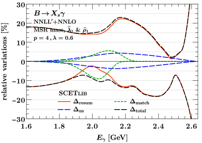
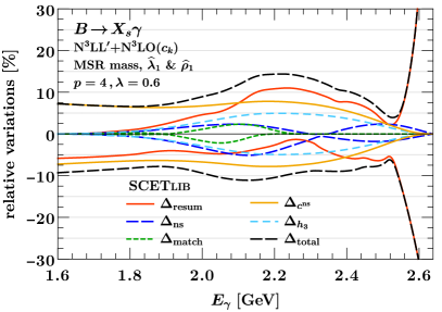
Figure -355: Breakdown of the perturbative uncertainty for the $B\to X_{s}\gamma$ spectrum into its components at NNLL${}^{\prime}+$NNLO (left panel) and N³LL${}^{\prime}+$N³LO$(c_{k})$ (right panel).

Our main predictions for the $B\to X_{s}\gamma$ photon energy spectrum at different perturbative orders are presented in figure -356. In addition to the colored bands showing $\Delta_{\rm profile}$, the gray dashed line shows $\Delta_{\rm profile}\oplus\Delta_{h_{3}}$, and the black solid line shows $\Delta_{\rm total}$ defined in eq. (4.2). The first column shows the results for the spectrum, and the second column shows the relative difference to the central value at the highest order, i.e. to the red solid line on the left. In the first row, we use the same value for the shape-function parameter $p=4$ for all orders, whereas in the second row, we use different values for $p$. In figure -355 we show the breakdown of the relative perturbative uncertainties into the individual contributions at NNLL${}^{\prime}+$NNLO and N³LL${}^{\prime}+$N³LO$(c_{k})$.

We remind the reader that the choice $p=4$ was needed to ensure that the spectrum at the highest order N³LL^′ still vanishes in the limit $E_{\gamma}\to m_{B}/2$. In practice, when fitting to the experimental data, the fit will always fix the precise shape near the endpoint to that of the data irrespective of the perturbative order, while the perturbative differences get moved (at least partially) into the fit result for $\mathcal{F}$. By using the same fixed model for $\mathcal{F}$ at each order, we can directly assess the perturbative convergence in the spectrum. However, by using a common $p$, the spectrum at lower orders vanishes correspondingly faster, i.e., quadratically at NNLL^′ and cubically at NLL^′, which also affects to some extent the shape of the spectrum into the peak. Therefore, in the lower panels of figure -356 we also show an alternative order comparison, where we do change the model at each order by using successively lower values for $p$ at the lower orders, such that the spectrum vanishes linearly at each order.

The results in figures -356 and -355 manifest a good perturbative convergence, especially from NNLL${}^{\prime}+$NNLO to N³LL${}^{\prime}+$N³LO$(c_{k})$. The relative uncertainties are under good control over the entire $E_{\gamma}$ range, except at the very endpoint where the spectrum vanishes so the relative uncertainties necessarily blow up. Apart from the very endpoint, the total uncertainty at N³LL${}^{\prime}+$N³LO$(c_{k})$ is at most 15% and in most of the $E_{\gamma}$ range well below that.

The uncertainties at N³LL${}^{\prime}+$N³LO$(c_{k})$ are substantially reduced compared to NNLL${}^{\prime}+$NNLO, even accounting for the fact that not all 3-loop perturbative ingredients are known. As expected, the higher-order uncertainties estimated from profile scale variations ($\Delta_{\rm resum}$, $\Delta_{\rm ns}$, $\Delta_{\rm match}$) are much reduced. Also recall that in the fixed-order tail $\Delta_{\rm resum}$ turns into the usual fixed-order scale variation. The uncertainty $\Delta_{h_{3}}$ is visible but subdominant. Across the entire peak of the spectrum, the uncertainty $\Delta_{c^{\rm ns}}$ from the missing 3-loop nonsingular corrections is at most comparable to the other sources thanks to the power suppression of the nonsingular. As expected, in the tail below $E_{\gamma}\lesssim E_{1}=2.1\,\mathrm{GeV}$ it starts to take over and becomes the dominant uncertainty. This demonstrates that in our approach we are able to substantially benefit from the increased precision of the N³LL^′ resummation even in the absence of the full N³LO result. Furthermore, in the fixed-order tail the total uncertainty dominated by $\Delta_{c^{\rm ns}}$ is still reduced compared to the scale-variation based estimate at NNLL${}^{\prime}+$NNLO. As discussed at the end of section 2.3, this is anticipated and justified because of the additional nontrivial perturbative information included at N³LO$(c_{k})$.

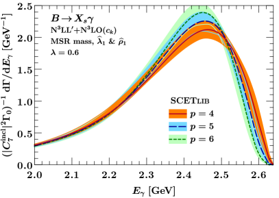
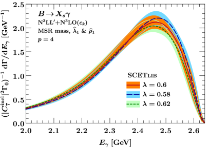
Figure -354: The $B\to X_{s}\gamma$ spectrum using different values for the shape-function parameters $p$ (left panel) and $\lambda$ (right panel) at N³LL${}^{\prime}+$N³LO$(c_{k})$. The remaining theory parameters are set to their default values.

The effect of varying the shape function model parameters $p$ and $\lambda$ is illustrated in figure -354. As expected, the position and height of the peak depend on the model parameters. We can clearly see how the value of $p$ controls how fast the spectrum vanishes toward the endpoint $E_{\gamma}\to m_{B}/2$. The value of $\lambda$ determines the width of shape function, which as a result controls the width of the peak. We stress that these results are just meant as an additional illustration. In particular, the differences seen in figure -354 are not to be interpreted as an additional theoretical uncertainty in the predictions. As mentioned before, the actual shape of $\mathcal{F}$ will be determined by fitting to the experimental data.

5.2 Different treatments of higher-order singular cross terms

When evaluating the singular correction using the factorization theorem in eq. (2.2) by default we expand the fixed-order boundary conditions of the hard, jet, and soft functions against each other. This is usually done, because it ensures that when switching off the resummation in the far-tail region and adding the fixed-order nonsingular correction, the fixed-order results are exactly reproduced. In ref. [15] it was observed that in the 1$S$ scheme and up to NNLL${}^{\prime}+$NNLO the perturbative convergence in the resummation region is substantially improved by keeping the hard function unexpanded as an overall factor. The main reason is that this ensures that the hard function does not affect the shape of the spectrum, which receives relatively large corrections from the jet and soft functions. The disadvantage is that this has the danger of generating unphysically large higher-order corrections in the fixed-order limit. In ref. [15] it was checked that this does not happen in the region of interest.

In this section, we study the differences in our perturbative setup between expanding the hard function against soft and jet functions (our default) vs. keeping it unexpanded.

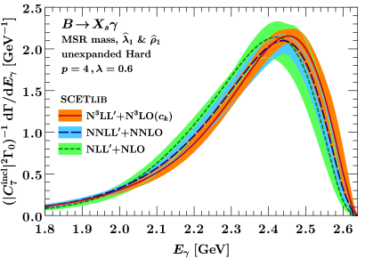
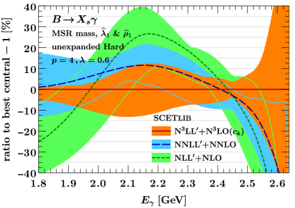
Figure -353: $B\to X_{s}\gamma$ spectrum with unexpanded hard function.

A priori, the additional higher-order terms induced by keeping the hard function unexpanded can easily spoil the delicate cancellation between singular and nonsingular contributions in the far tail of the spectrum. To fix this problem, we compensate for these higher-order terms by adding a constant term that cancels them in the fixed-order region but is only a power-suppressed correction in the peak region,

$$\Bigl{[}W_{77}^{\rm s}(k)+W_{77}^{\rm ns}(k)\Bigr{]}\to\Bigl{[}W_{77}^{\rm s,\mathrm{unexp}}(k)-W_{77,{\rm FO}}^{\rm s,\mathrm{unexp}}(\widehat{m}_{b})\Bigr{]}+\Bigl{[}W_{77}^{\rm ns}(k)+W_{77,{\rm FO}}^{\rm s,\mathrm{exp}}(\widehat{m}_{b})\Bigr{]}\,,$$ (5.1)

where we subtract the singular with unexpanded hard function, $W_{77,{\rm FO}}^{\rm s,\mathrm{unexp}}(\widehat{m}_{b})$ and add it back with expanded out hard function, $W_{77,{\rm FO}}^{\rm s,\mathrm{exp}}(\widehat{m}_{b})$. Both of these terms are evaluated at fixed order and at $k=\widehat{m}_{b}$, corresponding to the tail limit $x=1$, so in the peak region they are indeed power suppressed. This prescription allows us to take advantage of keeping the hard function unexpanded in the peak region while avoiding unphysically large corrections from higher-order cross terms in the fixed-order region, since they are explicitly removed in the $x\to 1$ limit.

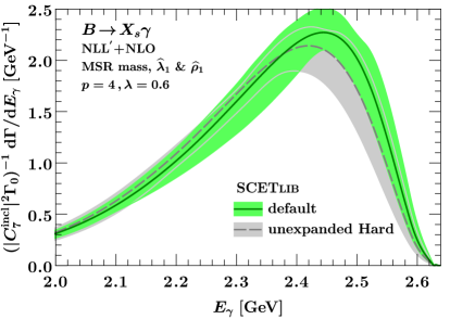
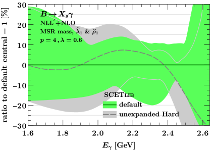
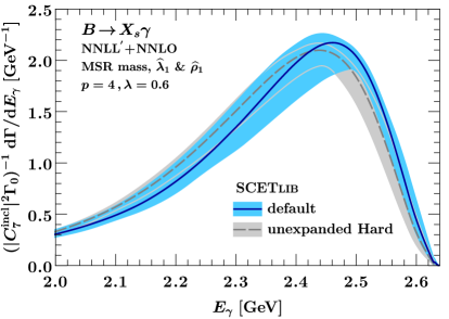
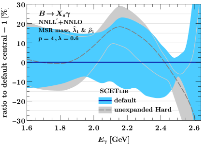
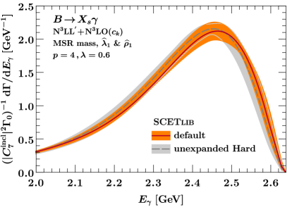
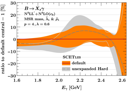
Figure -352: Comparison of $B\to X_{s}\gamma$ spectrum with expanded and unexpanded hard function. The colored and gray bands at each order display the spectrum with expanded and unexpanded hard function, respectively.

The numerical results using this prescription are shown in figure -353, where we adopt the MSR scheme with short-distance schemes for $\widehat{\lambda}_{1}$ and $\widehat{\rho}_{1}$. We compare these results to our default setup using the expanded hard function in figure -352. Here one can see that, overall, both scenarios lead to somewhat compatible results. Nevertheless, the choice of expanding the hard function or not clearly has a large impact at lower orders (which are expected to be more sensitive to the treatment of higher-order cross terms). Keeping the hard function unexpanded leads to a rather unnatural reduction of scale variations in the peak region of the spectrum. This behavior is quite dramatic at NNLL${}^{\prime}+$NNLO, where the uncertainty band with an unexpanded hard function (the gray band) barely captures the central line from the results with expanded hard function (solid blue line), and its size is almost as large as the scale variations at N³LL${}^{\prime}+$N³LO$(c_{k})$. This is also visible in figure -353, where the blue band suspiciously narrows down in the peak region of the spectrum and competes with the orange band. Based on this set of observations we conclude that in our setup keeping the hard function unexpanded is disfavored. Hence, for our final numerical results we opt for the conventional treatment of fully expanding the fixed-order boundary conditions of the hard, jet, and soft functions against each other, since it yields an overall more consistent picture of perturbative uncertainties and convergence.

5.3 Impact of short-distance schemes: 1$S$ vs. MSR mass schemes

As already explained in section 3 the right choice of short-distance scheme for the $b$-quark mass plays a key role in stabilizing the predictions at different orders in perturbation theory. In this section we illustrate the numerical impact of expressing $m_{b}$, $\lambda_{1}$, and $\rho_{1}$ in short-distance schemes. Moreover, we show that the 1$S$ mass scheme, which was successfully used in previous works [15, 32] up to NNLL${}^{\prime}+$NNLO, starts to break down at N³LL^′, while the MSR mass scheme yields convergent, stable results.

In the following figures we show our numerical predictions for the soft function (left column) and photon energy spectrum (right column) at different orders using the pole (figure -351), 1$S$ (figure -350 and figure -348), and MSR (figure -349) schemes. In these plots, we always use our default setup modulo the different short-distance schemes as indicated. For the soft function, we always show the combination $S(k,\mu_{0})\otimes U_{S}(k,\mu_{0},1.3\,\mathrm{GeV})$, i.e., we use the soft evolution kernel to evolve the soft function to a fixed scale $\mu=1.3\,\mathrm{GeV}$. In this way, the $\mu_{0}$ dependence cancels up to higher order, so we can use our default $\mu_{0}$ variations to estimate the perturbative uncertainties for the soft function.

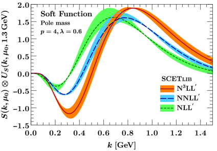
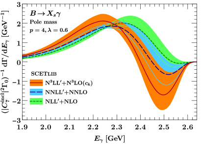
Figure -351: The soft function (left panel) and the $B\to X_{s}\gamma$ spectrum (right panel) at different orders in the pole mass scheme. Small values of $k$ in the soft function correspond to large $E_{\gamma}$ in the spectrum. The pole-mass renormalon leads to the large negative dip at small $k$ and large $E_{\gamma}$ and an unstable position of the peak.

In figure -351 we clearly see that the soft function in the pole scheme suffers from a sizable renormalon ambiguity, which is intrinsic to the pole scheme, leading to a large negative deep before the peak. Moreover, the peak position varies significantly from one order to another, which reflects the instabilities in the first moments of the shape function. All these features are also mirrored in the corresponding results for the spectrum. This behaviour of the pole scheme was already observed in ref. [32] up to NNLL^′, and we see that it continues to get worse at N³LL^′.

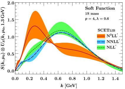
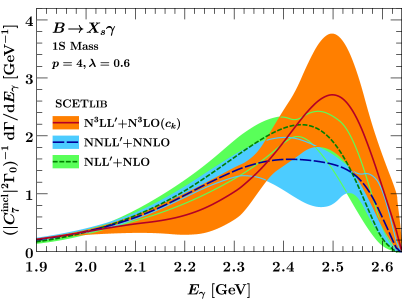
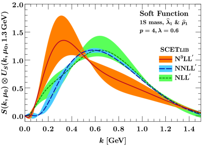
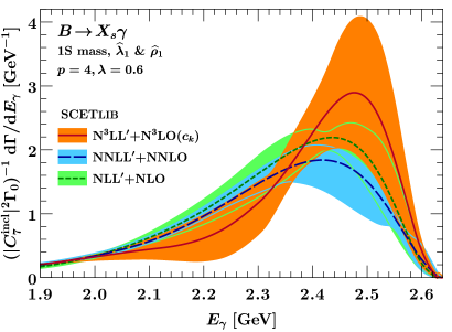
Figure -350: The soft function (left panel) and the $B\to X_{s}\gamma$ spectrum (right panel) in the 1$S$ mass scheme. The top panels use the pole scheme for $\lambda_{1}$ and $\rho_{1}$, while the bottom panels use a short-distance scheme. In both cases the spectrum, and in particular the position of its peak, are stable at NLL${}^{\prime}+$NLO and NNLL${}^{\prime}+$NNLO, but at N³LL${}^{\prime}+$N³LO$(c_{k})$ the predictions start breaking down.

The predictions in the 1$S$ mass scheme are presented in figure -350. Although the differential decay rate up to NNLL^′ is somewhat stable, the prediction fails dramatically at N³LL^′. In particular, the uncertainty band from scale variation is completely out of control. Adopting short-distance schemes for $\lambda_{1}$ and $\rho_{1}$ slightly improves the spectrum up to NNLL${}^{\prime}+$NNLO, but the picture at N³LL${}^{\prime}+$N³LO$(c_{k})$ does not change. Neither does it seem to be possible to substantially improve the convergence by adjusting the values of the residual short-distance coefficients $\delta\lambda_{1}^{(2)}$, $\delta\lambda_{1}^{(3)}$, and $\delta\rho_{1}^{(3)}$. Keeping the hard function unexpanded in the 1$S$ scheme somewhat improves the picture up to NNLL${}^{\prime}+$NNLO but does not help at all with the bad behaviour at N³LL${}^{\prime}+$N³LO$(c_{k})$.

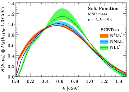
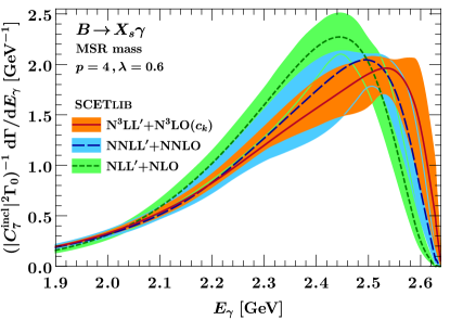
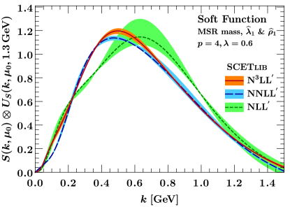
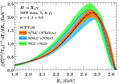
Figure -349: The soft function (left panel) and the $B\to X_{s}\gamma$ spectrum (right panel) in the MSR mass scheme. The top panels use the pole scheme for $\lambda_{1}$ and $\rho_{1}$, while the bottom panels use a short-distance scheme. The convergence is significantly better than in the other mass schemes, and is further improved by adoption of short-distance schemes for $\lambda_{1}$ and $\rho_{1}$.

The results in the MSR scheme are presented in figure -349. In this case we observe much more stable results in comparison to the 1$S$ scheme. Here in the first row, where we only switch the $b$-quark mass to the MSR scheme, we still observe that the spectrum is very sensitive to the behavior of the soft function at small $k$. This sensitivity is reflected in the uncertainty estimates from scale variation. By subtracting the subleading renormalons present in $\lambda_{1}$ and $\rho_{1}$, we find a substantial improvement in the peak region of the spectrum, and the result exhibits excellent convergence between all orders (second row). From these results we can conclude that the MSR scheme is indeed a much more suitable mass scheme for the $B\to X_{s}\gamma$ spectrum when going beyond NNLL^′.

To understand the reason for the breakdown of the 1$S$ scheme at N³LL^′ we recall the relation between the pole and 1$S$ schemes up to the 3-loop order,

$$m_{b}^{\rm pole}=m_{b}^{1S}+R^{1S}(\mu)\sum_{n=1}^{3}\sum_{m=0}^{n-1}c_{nm}^{1S}\Bigl{[}\frac{\alpha_{s}(\mu)}{4\pi}\Bigr{]}^{n}\Bigl{[}\ln\frac{\mu}{R^{1S}(\mu)}\Bigr{]}^{m}\,.$$ (5.2)

where $R^{1S}(\mu)=C_{F}\,m_{b}^{1S}\alpha_{s}(\mu)$ is the built-in infrared cutoff scale of the 1$S$ scheme. The numerical values for the $c_{nm}$ coefficients are

$$c^{1S}_{10} =2.0944\,,$$

$$c^{1S}_{20} =135.438-10.2393\,n_{f}\,,$$

$$c^{1S}_{21} =92.1534-5.58505\,n_{f}\,,$$

$$c^{1S}_{30} =11398.2-1372.75\,n_{f}+38.9677\,n_{f}^{2}\,,$$

$$c^{1S}_{31} =7766.02-1077.92\,n_{f}+33.5103\,n_{f}^{2}\,,$$

$$c^{1S}_{32} =3041.06-368.614\,n_{f}+11.1701\,n_{f}^{2}\,.$$ (5.3)

By contrast to the MSR scheme where the $R$ scale is a parameter we can choose, in the 1$S$ scheme $R^{1S}(\mu)$ depends on the renormalization scale $\mu$ via the coupling constant. Hence its size increases when decreasing the scale $\mu$, e.g. at hard scale we find $R^{1S}(4.75\,\mathrm{GeV})=1.36\,\mathrm{GeV}$, whereas at the soft scale we obtain $R^{1S}(\mu_{S}=1.3\,\mathrm{GeV})=2.40\,\mathrm{GeV}$, which is almost twice the size of the soft scale itself. Such a large infrared scale violates the power counting of HQET that is used to describe the heavy quarks in the $B$ meson with the residual soft momenta $k\sim\Lambda_{\rm QCD}$ in the peak region.

The mismatch between the size of $R^{1S}$ and $\mu_{S}\sim k$ not only breaks the power counting of the EFT description of the decay rate, but also spoils the renormalon subtraction in the soft function. To see this explicitly, we consider the conversion between the 1$S$ and MSR schemes $\Delta m_{b}(R)\equiv m_{b}^{\rm MSR}(R)-m_{b}^{1S}$, which formally does not involve a renormalon. We obtain the following perturbative series for $\Delta m_{b}(R=\mu)$ at various scales,

$$\Delta m_{b}(R=\mu)\Big{|}_{\mu=4.2\,\mathrm{GeV}} =-0.35\,\epsilon-0.12\,\epsilon^{2}-0.04\,\epsilon^{3}~{}[\!\,\mathrm{GeV}]\,,$$

$$\Delta m_{b}(R=\mu)\Big{|}_{\mu=1.93\,\mathrm{GeV}} =-0.15\,\epsilon-0.06\,\epsilon^{2}+0.02\,\epsilon^{3}~{}[\!\,\mathrm{GeV}]\,,$$

$$\Delta m_{b}(R=\mu)\Big{|}_{\mu=1.3\,\mathrm{GeV}} =-0.06\,\epsilon-0.06\,\epsilon^{2}+0.10\,\epsilon^{3}~{}[\!\,\mathrm{GeV}]\,,$$ (5.4)

where $\epsilon\equiv 1$ is an auxiliary parameter denoting the perturbative order of the corrections. The perturbative series in the first line shows a rather good convergence for $\Delta m_{b}$ at the hard scale. However, in this regime the perturbative expansion for the 1$S$ scheme contains large logarithms of the form $\ln(\mu/R^{1S}(\mu))|_{\mu=4.7\,\mathrm{GeV}}\sim\ln(4.7/1.36)$. These logarithms are suppressed by $R^{1S}(\mu=m_{b}^{1S})/m_{b}^{1S}=1.36/4.7$ and are therefore harmless in the fixed-order expansion. For example, in the context of calculating the total decay rate, it is well-known that the 1$S$ scheme provides a good description for the bottom mass.

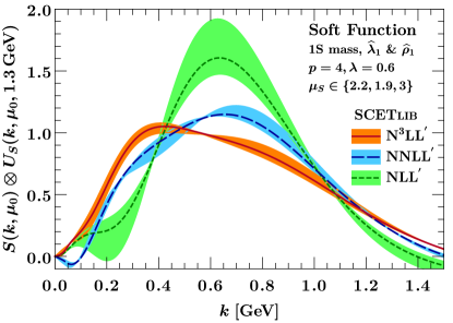
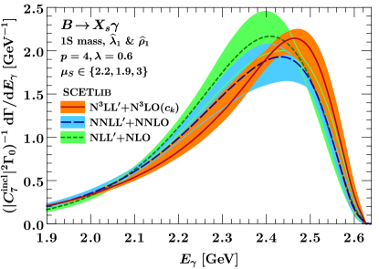
Figure -348: The soft function (left panel) and the $B\to X_{s}\gamma$ spectrum (right panel) in the 1$S$ mass scheme. A short-distance scheme is used for the hadronic parameters $\lambda_{1}$ and $\rho_{1}$. In contrast to the other plots, larger values are used for the soft scale: $\mu_{0}\in\{2.2,1.9,3\}\,\mathrm{GeV}$. The larger soft scale amends the breakdown of 1$S$ scheme at N³LL${}^{\prime}+$N³LO$(c_{k})$, but is not compatible with the SCET scale hierarchy.

We can also define a natural scale for the 1$S$ scheme, which we denote as $\mu_{1S}$, at which all logarithms of the form $\ln(\mu_{1S}/R^{1S}(\mu_{1S}))$ are resummed. It corresponds to the fixed point of the $R^{1S}$ scale where $R^{1S}(\mu_{1S})=\mu_{1S}$, which yields $\mu_{1S}=1.93\,\mathrm{GeV}$. The perturbative series for $\Delta m_{b}(\mu_{1S})$ is shown in the second line of eq. (5.3). It shows the same good convergence as the first line, but with overall smaller corrections and a change of sign in the $\mathcal{O}(\epsilon^{3})$ coefficient.

Finally, the last line in eq. (5.3) shows the perturbative series for $\Delta m_{b}(\mu_{S})$ at the soft scale $\mu_{S}=1.3\,\mathrm{GeV}$. As one can see, the resulting series exhibits no convergence and breaks down at the 3-loop order. This behavior vividly explains the failure of the 1$S$ mass scheme when used at the soft scale to remove the renormalon in the soft function.

Another interesting conclusion from the discussion above is that one can retain the use of the 1$S$ scheme as soon as the actual soft scale in the problem is roughly of the same order of $R^{1S}=\mu_{1S}\sim 1.93\,\mathrm{GeV}$. To examine this hypothesis, in figure -348 we show the results for the soft function and the photon energy spectrum in the 1$S$ mass scheme where the soft scale is chosen to have larger values, $\mu_{S}\in\{2.2,1.9,3\}\,\mathrm{GeV}$. Indeed the resulting spectrum exhibits a significant improvement at all orders compared to figure -350, and in particular the N³LL${}^{\prime}+$N³LO$(c_{k})$ result is now much more well behaved. However, in practice this setup is not really ideal since the soft scale is now much larger than $\Lambda_{\rm QCD}$ and our default soft scale, which leads to rather large unresummed logarithms in the soft function. Consequently, the results in figure -348 do not reach the same level of stability as those in the MSR scheme in figure -349.

6 Conclusions

In this paper, we presented the photon energy spectrum in $B\to X_{s}\gamma$ at N³LL${}^{\prime}+$N³LO$(c_{k})$, mediated by the electromagnetic operator in the weak Hamiltonian. For the singular contributions we used the SCET factorization theorem to resum large logarithms, which arise in the description of the spectrum close to the kinematic endpoint. We accounted for the complete soft and jet functions at $\rm N^{3}LO$ and treated the unknown nonlogarithmic constant of the 3-loop hard function as a nuisance parameter. In addition, the RG evolution is performed at complete N³LL, taking advantage of the fully-known 3-loop anomalous dimensions. We matched the resummed predictions to fixed order at the formal N³LO order, developing a method that allows us to consistently include the known NNLO results, while parametrizing the missing nonsingular corrections at 3-loop order in terms of suitable theory nuisance parameters $c_{k}$. The variation of these nuisance parameters provides an estimate of the uncertainty that arises from our ignorance of these missing terms.

We incorporated nonperturbative effects by convolving the partonic spectrum with a universal shape function. The first moments of the shape function depend on the $b$-quark mass $m_{b}$ and the HQET parameters $\lambda_{1}$ and $\rho_{1}$. It is crucial to define these parameters in a suitable short-distance scheme to avoid renormalon ambiguities that would spoil the convergence of perturbative series. Another important aspect of our analysis was the implementation and choice of an appropriate short-distance scheme at N³LL^′. By using the MSR mass scheme for $m_{b}$ and adopting an analogous scheme to the “invisible” scheme for $\lambda_{1}$ and $\rho_{1}$ we are able to obtain stable predictions. We also find, quite unexpectedly, that the 1$S$ mass scheme, which has been successfully used in the past for this process up to NNLL^′, starts to badly break down at N³LL${}^{\prime}+$N³LO$(c_{k})$. We demonstrated that the reason for this sudden breakdown is that the 1$S$ scheme is ultimately not designed for use at very low scales. This is because its built-in infrared cutoff scales with $\alpha_{s}(\mu)$ and thus increases at lower scales and quickly becomes too large when the soft scale is lower than $\mu_{1S}=1.93\,\mathrm{GeV}$, such that it effectively breaks the power counting of the underlying HQET.

Our main results are presented in section 5.1. Our final predictions for the photon energy spectrum in the MSR scheme and invisible schemes for $\lambda_{1}$ and $\rho_{1}$ exhibit excellent perturbative stability, in particular considering the rather low scales involved in the problem. In particular, we observe a substantial improvement of the perturbative theory uncertainties from NNLL${}^{\prime}+$NNLO to N³LL${}^{\prime}+$N³LO$(c_{k})$. Importantly, even without the complete fixed $\mathcal{O}(\alpha_{s}^{3})$ information available, with our method we are able to benefit from the increased perturbative precision at N³LL^′, allowing us to improve the precision of the theory predictions across the entire phenomenologically important peak region. Indeed, the uncertainties due to the missing fixed-order results at $\mathcal{O}(\alpha_{s}^{3})$ only become dominant in the fixed-order tail of the spectrum, which is phenomenologically less relevant. Nevertheless, their calculation is still encouraged and needed to further reduce the theory uncertainties.

In the future, we look forward to confronting our improved predictions with both existing and future experimental measurements, enabling more precise determinations of the shape function $\mathcal{F}(k)$, the $b$-quark mass, and the normalization of the $B\to X_{s}\gamma$ rate.

Appendix A Resummation ingredients

A.1 General definitions

We write the perturbative series for the cusp and noncusp anomalous dimensions as

$$\Gamma_{\mathrm{cusp}}(\alpha_{s})\equiv\Gamma_{\mathrm{cusp}}^{q}(\alpha_{s})=\sum_{n=0}^{\infty}\Gamma_{n}\Bigl{(}\frac{\alpha_{s}}{4\pi}\Bigr{)}^{n+1}\,,\qquad\gamma^{F}(\alpha_{s})=\sum_{n=0}^{\infty}\gamma_{n}^{F}\Bigl{(}\frac{\alpha_{s}}{4\pi}\Bigr{)}^{n+1}\,.$$ (A.1)

At N³LL^′, we need the quark cusp anomalous coefficients up to four loops [52, 53, 54, 55]. The coefficients $\beta_{n}$ of the QCD $\beta$ function in $\overline{\text{MS}}$ are defined as

$$\frac{\mathrm{d}\alpha_{s}(\mu)}{\mathrm{d}\ln\mu}=\beta\bigl{[}\alpha_{s}(\mu)\bigr{]}=-2\alpha_{s}(\mu)\sum_{n=0}^{\infty}\beta_{n}\,\biggl{[}\frac{\alpha_{s}(\mu)}{4\,\pi}\biggr{]}^{n+1}\,.$$ (A.2)

At N³LL^′ they are also needed up to four loops [56, 57, 58, 59].

The RGE solutions are written in terms of the following standard integrals

$$K_{\Gamma}(\mu_{0},\mu) =\int_{\alpha_{s}(\mu_{0})}^{\alpha(\mu)}\frac{\mathrm{d}\alpha_{s}}{\beta(\alpha_{s})}\,\Gamma_{\mathrm{cusp}}(\alpha_{s})\int_{\alpha_{s}(\mu_{0})}^{\alpha_{s}}\frac{\mathrm{d}\alpha_{s}^{\prime}}{\beta(\alpha_{s}^{\prime})}\,,$$

$$\eta_{\Gamma}(\mu_{0},\mu) =\int_{\alpha_{s}(\mu_{0})}^{\alpha_{s}(\mu)}\frac{\mathrm{d}\alpha_{s}}{\beta(\alpha_{s})}\,\Gamma_{\mathrm{cusp}}(\alpha_{s})\,,$$

$$K_{\gamma}(\mu_{0},\mu) =\int_{\alpha_{s}(\mu_{0})}^{\alpha_{s}(\mu)}\frac{\mathrm{d}\alpha_{s}}{\beta(\alpha_{s})}\,\gamma(\alpha_{s})\,.$$ (A.3)

In principle, they can be performed analytically [60]. For simplicity, in our numerical results we employ the standard approximate analytic solutions [61], which are obtained by performing the integrals after expanding the numerators in $\alpha_{s}$. For our purposes here, the numerical accuracy of the approximate analytic solutions is sufficient [61].

Following ref. [32], we define the plus distributions

$$\mathcal{L}_{-1}(x) =\delta(x)\,,$$

$$\mathcal{L}_{n}(x) =\biggl{[}\frac{\theta(x)\ln^{n}x}{x}\biggr{]}_{+}=\lim_{\epsilon\to 0}\,\frac{\mathrm{d}}{\mathrm{d}x}\,\biggl{[}\theta(x-\epsilon)\,\frac{\ln^{n+1}x}{n+1}\biggr{]}\qquad(n\geq 0)\,,$$

$$\mathcal{L}^{a}(x) =\biggl{[}\frac{\theta(x)}{x^{1-a}}\biggr{]}_{+}=\lim_{\epsilon\to 0}\,\frac{\mathrm{d}}{\mathrm{d}x}\,\biggl{[}\theta(x-\epsilon)\,\frac{x^{a}-1}{a}\biggr{]}\,.$$ (A.4)

A.2 Hard function

We write the perturbative series for the hard function in the pole-mass scheme as

$$h_{s}(m_{b}^{\rm pole},\mu)=\sum_{n=0}^{\infty}\sum_{m=0}^{2\,n}\,H_{m}^{(n)}\biggl{[}\frac{\alpha_{s}(\mu)}{4\,\pi}\biggr{]}^{n}\ln^{m}\Bigl{(}\frac{\mu}{m_{b}^{\rm pole}}\Bigr{)}\,.$$ (A.5)

It satisfies the following RGE,

$$\frac{\mathrm{d}h_{s}(m_{b}^{\rm pole},\mu)}{\mathrm{d}\ln\mu}=\biggl{\{}\Gamma^{H}[\alpha_{s}(\mu)]\ln\frac{\mu}{m_{b}^{\rm pole}}+\gamma^{H}[\alpha_{s}(\mu)]\biggr{\}}h_{s}(m_{b}^{\rm pole},\mu)\,,$$ (A.6)

where $\Gamma^{H}(\alpha_{s})\equiv-2\Gamma_{\mathrm{cusp}}(\alpha_{s})$ and $\gamma^{H}(\alpha_{s})=2\gamma^{q}(\alpha_{s})+2\gamma^{Q}(\alpha_{s})$ are the hard cusp and noncusp anomalous dimensions. The noncusp anomalous coefficients $\gamma_{n}^{H}=2\gamma_{n}^{q}+2\gamma_{n}^{Q}$ are known to three loops [23].

The nonlogarithmic coefficients of the hard function in eq. (A.5) are known to two loops [39, 32],

$$H^{(0)}_{0} =1\,,$$

$$H^{(1)}_{0} =-C_{F}\biggl{(}12+\frac{\pi^{2}}{6}\biggr{)}\,,$$

$$H^{(2)}_{0} =16\,C_{F}\,\biggl{[}3.88611\,C_{F}+5.89413\,C_{A}-\biggl{(}\frac{7859}{3456}+\frac{109\pi^{2}}{576}+\frac{13\zeta_{3}}{48}\biggr{)}\beta_{0}$$

$$\quad+\frac{3563}{1296}-\frac{29\pi^{2}}{108}-\frac{\zeta_{3}}{6}\biggr{]}\,,$$ (A.7)

The 3-loop coefficient $H^{(3)}_{0}$ is currently unknown and treated as a nuisance parameter as discussed in section 2.2, where $h_{n}\equiv H_{0}^{(n)}/4^{n}$.

The coefficients of the logarithmic terms $H^{(n)}_{m\geq 1}$ are determined by iteratively solving the RGE in eq. (A.6) order by order. Substituting eq. (A.5) into eq. (A.6), we obtain a recurrence relation that expresses them in terms of the anomalous dimensions and lower-order nonlogarithmic coefficients,

$$H^{(n)}_{m}=\frac{1}{\,m}\biggl{\{}\sum_{j=0}^{t_{1}}\bigl{(}\gamma^{H}_{j}+2\,(n-j-1)\,\beta_{j}\bigr{)}\,H^{(n-j-1)}_{m-1}+\theta(m\geq 2)\sum_{j=0}^{t_{2}}\Gamma_{j}^{H}\,H^{(n-j-1)}_{m-2}\biggr{\}}\,,\quad m\geq 1$$ (A.8)

with summation limits $t_{1}=\lfloor n-(m+1)/2\rfloor$ and $t_{2}=\lfloor n-m/2\rfloor$, where the symbol $\lfloor\rfloor$ denotes the floor function. The condition $\theta(m\geq 2)$ indicates that the second sum is present only if $m\geq 2$. The explicit expressions up to three loops read

$$H^{(1)}_{1} =\gamma_{0}^{H}\,,$$

$$H^{(1)}_{2} =\frac{1}{2}\,\Gamma_{0}^{H}\,,$$

$$H^{(2)}_{1} =H_{0}^{(1)}\,\bigl{(}2\,\beta_{0}+\gamma^{H}_{0}\bigr{)}+\gamma^{H}_{1}\,,$$

$$H^{(2)}_{2} =\frac{1}{2}\,\Bigl{\{}2\,\beta_{0}\,\gamma_{0}^{H}+\bigl{(}\gamma_{0}^{H}\bigr{)}^{2}+H_{0}^{(1)}\Gamma^{H}_{0}+\Gamma^{H}_{1}\Bigr{\}}\,,$$

$$H^{(2)}_{3} =\frac{1}{6}\,\Gamma_{0}^{H}\,\bigl{(}2\,\beta_{0}+3\,\gamma^{H}_{0}\bigr{)}\,,$$

$$H^{(2)}_{4} =\frac{1}{8}\,\bigl{(}\Gamma_{0}^{H}\bigr{)}^{2}\,,$$

$$H^{(3)}_{1} =H_{0}^{(2)}\,\bigl{(}4\,\beta_{0}+\gamma_{0}^{H}\bigr{)}+H_{0}^{(1)}\,\bigl{(}2\,\beta_{1}+\gamma_{1}^{H}\bigr{)}+\gamma_{2}^{H}\,,$$

$$H^{(3)}_{2} =\frac{1}{2}\,\Bigl{\{}2\,\beta_{1}\,\gamma_{0}^{H}+4\,\beta_{0}\,\gamma_{1}^{H}+2\,\gamma_{0}^{H}\,\gamma_{1}^{H}+H_{0}^{(2)}\Gamma_{0}^{H}$$

$$\quad+H_{0}^{(1)}\,\Bigl{(}8\,\beta_{0}^{2}+6\,\beta_{0}\,\gamma_{0}^{H}+\bigl{(}\gamma_{0}^{H}\bigr{)}^{2}+\Gamma_{1}^{H}\Bigr{)}+\Gamma_{2}^{H}\Bigr{\}}\,,$$

$$H^{(3)}_{3} =\frac{1}{6}\,\Bigl{\{}8\,\beta_{0}^{2}\,\gamma_{0}^{H}+\bigl{(}\gamma_{0}^{H}\bigr{)}^{3}+\bigl{(}2\,\beta_{1}+3\,\gamma_{1}^{H}\bigr{)}\,\Gamma^{H}_{0}+3\,\gamma^{H}_{0}\,\bigl{(}H_{0}^{(1)}\,\Gamma_{0}^{H}+\Gamma_{1}^{H}\bigr{)}$$

$$\quad+\beta_{0}\,\Bigl{(}6\,\bigl{(}\gamma_{0}^{H}\bigr{)}^{2}+8\,H_{0}^{(1)}\,\Gamma_{0}^{H}+4\,\Gamma_{1}^{H}\Bigr{)}\Bigr{\}}\,,$$

$$H^{(3)}_{4} =\frac{1}{24}\,\Gamma_{0}^{H}\,\bigl{(}8\,\beta_{0}^{2}+20\,\beta_{0}\,\gamma^{H}_{0}+6\,\bigl{(}\gamma^{H}_{0}\bigr{)}^{2}+3\,H_{0}^{(1)}\Gamma_{0}^{H}+6\,\Gamma_{1}^{H}\bigr{)}\,,$$

$$H^{(3)}_{5} =\frac{1}{24}\,\bigl{(}\Gamma_{0}^{H}\bigr{)}^{2}\,\bigl{(}4\,\beta_{0}+3\,\gamma_{0}^{H}\bigr{)}\,,$$

$$H^{(3)}_{6} =\frac{1}{48}\bigl{(}\Gamma_{0}^{H}\bigr{)}^{3}\,.$$ (A.9)

The all-order solution of the RGE in eq. (A.6) is given by

$$h_{s}(m_{b}^{\rm pole},\mu) =h_{s}(m_{b}^{\rm pole},\mu_{H})\,U_{H}(m_{b}^{\rm pole},\mu_{H},\mu)\,,$$ (A.10)

$$U_{H}(m_{b},\mu_{H},\mu) =\exp\biggl{[}-2K_{\Gamma}(\mu_{H},\mu)-2\eta_{\Gamma}(\mu_{H},\mu)\ln\frac{\mu_{H}}{m_{b}}+K_{\gamma^{H}}(\mu_{H},\mu)\biggr{]}\,.$$

A.3 Jet function

The perturbative series for the renormalized jet function reads

$$J(s,\mu)=\sum_{n=0}^{\infty}\sum_{m=-1}^{2n-1}J^{(n)}_{m}\biggl{[}\frac{\alpha_{s}(\mu)}{4\pi}\biggr{]}^{n}\frac{1}{\mu^{2}}\,\mathcal{L}_{m}\Bigl{(}\frac{s}{\mu^{2}}\Bigr{)}\,,\,.$$ (A.11)

The jet function is normalized such that $J^{(n)}_{-1}=1$. Explicit expressions for the coefficients $J^{(n)}_{m}$ up to 3-loop order in our notation are given in refs. [62, 22].

For completeness, the jet function obeys the RGE

$$\frac{\mathrm{d}J(s,\mu)}{\mathrm{d}\ln\mu}=\biggl{\{}\Gamma^{J}[\alpha_{s}(\mu)]\frac{1}{\mu^{2}}\,\mathcal{L}_{0}\Bigl{(}\frac{s}{\mu^{2}}\Bigr{)}+\gamma^{J}[\alpha_{s}(\mu)]\,\delta(s)\biggr{\}}\otimes_{s}J(s,\mu)$$ (A.12)

where $\Gamma^{J}(\alpha_{s})=-2\Gamma_{\mathrm{cusp}}(\alpha_{s})$ and the symbol $\otimes_{s}$ denotes the convolution of the form

$$f(s)\otimes_{s}g(s)=\int\mathrm{d}s^{\prime}\,f(s-s^{\prime})\,g(s^{\prime})\,.$$ (A.13)

In our numerical implementation, we do not need to explicitly solve the jet-function RGE, because we always evolve the hard and soft functions to the jet scale.

A.4 Partonic soft function

In the pole scheme the partonic soft function $C_{0}(\omega,\mu)$ is given by the $b$-quark matrix element

$$C_{0}(\omega,\mu)=\langle b_{v}|\bar{b}_{v}\delta(iD_{+}+\omega)b_{v}|b_{v}\rangle\,.$$ (A.14)

Its perturbative expansion is written as

$$C_{0}(\omega,\mu)=\sum_{n=0}^{\infty}\sum_{m=-1}^{2n-1}S^{(n)}_{m}\biggl{[}\frac{\alpha_{s}(\mu)}{4\pi}\biggr{]}^{n}\frac{1}{\mu}\,\mathcal{L}_{m}\Bigl{(}\frac{\omega}{\mu}\Bigr{)}\,.$$ (A.15)

The expansion coefficients $S_{m}^{(n)}$ can be found in ref. [23].

The RGE for the soft function reads

$$\frac{\mathrm{d}C_{0}(\omega,\mu)}{\mathrm{d}\ln\mu}=\biggl{\{}\Gamma^{S}[\alpha_{s}(\mu)]\frac{1}{\mu}\,\mathcal{L}_{0}\Bigl{(}\frac{\omega}{\mu}\Bigr{)}+\gamma^{S}[\alpha_{s}(\mu)]\,\delta(\omega)\biggr{\}}\otimes_{\omega}C_{0}(\omega,\mu)\,,$$ (A.16)

where $\Gamma^{S}(\alpha_{s})=2\Gamma_{\mathrm{cusp}}(\alpha_{s})$ and the noncusp anomalous coefficients are known to three loops [23]. By solving it iteratively, we can obtain a recurrence relation for all logarithmic coefficients $S^{(n)}_{m\geq 0}$,

$$S^{(n)}_{m}=-\frac{1}{m+\delta_{m0}}\biggl{\{}\sum_{j=0}^{t_{1}}\bigl{[}\gamma^{S}_{j}+2\,(n-j-1)\beta_{j}\bigr{]}\,S^{(n-j-1)}_{m-1}+\sum_{j=0}^{t_{2}}\sum_{i=t_{\rm m}-2}^{2(n-j)-3}\,\Gamma^{S}_{j}V^{0i}_{m-1}\,S^{(n-j-1)}_{i}\biggr{\}}\,,$$ (A.17)

where the summation limits are $t_{1}=\lfloor n-1-m/2\rfloor\,,t_{2}=\lfloor n-(t_{m}+1)/2\rfloor$ and $t_{\rm m}=\max{(m,1)}$. The coefficients $V^{mn}_{k}$ appear in the convolution algebra of plus distributions,

$$\mathcal{L}_{n}(x)\otimes_{x}\mathcal{L}_{m}(x)=\sum_{\mathclap{k=-1}}^{\mathclap{n+m+1}}V_{k}^{nm}\,\mathcal{L}_{k}(x)\,,$$ (A.18)

and are given in ref. [32]. It is easy to check that eq. (A.17) reproduces the explicit results to three loops in ref. [23].

The all-order solution of the soft RGE is [63, 64, 65, 32]

$$C_{0}(\omega,\mu) =C_{0}(\omega,\mu_{S})\otimes_{\omega}U_{S}(\omega,\mu_{S},\mu)\,,$$

$$U_{S}(\omega,\mu_{S},\mu) =\exp\Bigl{[}-2K_{\Gamma}(\mu_{S},\mu)+K_{\gamma^{S}}(\mu_{S},\mu)\Bigr{]}\mathcal{V}[2\eta_{\Gamma}(\mu_{S},\mu),\mu_{S},\omega]\,,$$

$$\mathcal{V}(\eta,\mu,\omega) =\frac{e^{-\gamma_{E}\eta}}{\Gamma(1+\eta)}\biggl{[}\frac{\eta}{\mu}\mathcal{L}^{\eta}\Bigl{(}\frac{\omega}{\mu}\Bigr{)}+\delta(\omega)\biggr{]}$$ (A.19)

where $K_{\Gamma}$, $\eta_{\Gamma}$, $K_{\gamma}$ are defined in eq. (A.1), $\gamma_{E}$ is the Euler-Mascheroni constant, and the $\mathcal{L}^{\eta}(x)$ plus distribution is defined in eq. (A.1).

Note that in the short-distance schemes we consider, the residual terms $\delta m_{b}$, $\delta\lambda_{1}$, $\delta\rho_{1}$ are formally $\mu$ independent, such that the evolution for the partonic soft function in a short-distance scheme $\widehat{C}_{0}(\omega,\mu)$ is the same as in the pole scheme.

References

- [1] S. Bertolini, F. Borzumati and A. Masiero, QCD Enhancement of Radiative b Decays, Phys. Rev. Lett. 59 (1987) 180.
- [2] B. Grinstein, R. P. Springer and M. B. Wise, Effective Hamiltonian for Weak Radiative B Meson Decay, Phys. Lett. B 202 (1988) 138.
- [3] M. Misiak et al., Estimate of at , Phys. Rev. Lett. 98 (2007) 022002 [hep-ph/0609232].
- [4] M. Misiak et al., Updated NNLO QCD predictions for the weak radiative B-meson decays, Phys. Rev. Lett. 114 (2015) 221801 [1503.01789].
- [5] B. Grinstein and M. B. Wise, Weak Radiative B Meson Decay as a Probe of the Higgs Sector, Phys. Lett. B 201 (1988) 274.
- [6] W.-S. Hou and R. S. Willey, Effects of Charged Higgs Bosons on the Processes , and , Phys. Lett. B 202 (1988) 591.
- [7] M. Misiak and M. Steinhauser, Weak radiative decays of the B meson and bounds on in the Two-Higgs-Doublet Model, Eur. Phys. J. C 77 (2017) 201 [1702.04571].
- [8] M. Neubert, Analysis of the photon spectrum in inclusive decays, Phys. Rev. D 49 (1994) 4623 [hep-ph/9312311].
- [9] I. I. Y. Bigi, M. A. Shifman, N. G. Uraltsev and A. I. Vainshtein, On the motion of heavy quarks inside hadrons: Universal distributions and inclusive decays, Int. J. Mod. Phys. A 9 (1994) 2467 [hep-ph/9312359].
- [10] M. Neubert, QCD based interpretation of the lepton spectrum in inclusive decays, Phys. Rev. D 49 (1994) 3392 [hep-ph/9311325].
- [11] BaBar collaboration, B. Aubert et al., Measurement of the branching fraction and photon energy spectrum using the recoil method, Phys. Rev. D 77 (2008) 051103 [0711.4889].
- [12] Belle collaboration, A. Limosani et al., Measurement of Inclusive Radiative B-meson Decays with a Photon Energy Threshold of 1.7-GeV, Phys. Rev. Lett. 103 (2009) 241801 [0907.1384].
- [13] BaBar collaboration, J. P. Lees et al., Measurement of B(), the photon energy spectrum, and the direct CP asymmetry in decays, Phys. Rev. D 86 (2012) 112008 [1207.5772].
- [14] BaBar collaboration, J. P. Lees et al., Exclusive Measurements of Transition Rate and Photon Energy Spectrum, Phys. Rev. D 86 (2012) 052012 [1207.2520].
- [15] SIMBA collaboration, F. U. Bernlochner, H. Lacker, Z. Ligeti, I. W. Stewart, F. J. Tackmann and K. Tackmann, Precision Global Determination of the Decay Rate, Phys. Rev. Lett. 127 (2021) 102001 [2007.04320].
- [16] C. W. Bauer and A. V. Manohar, Shape function effects in and decays, Phys. Rev. D 70 (2004) 034024 [hep-ph/0312109].
- [17] K. S. M. Lee and I. W. Stewart, Shape-function effects and split matching in , Phys. Rev. D 74 (2006) 014005 [hep-ph/0511334].
- [18] K. S. M. Lee, Z. Ligeti, I. W. Stewart and F. J. Tackmann, Universality and cut effects in , Phys. Rev. D 74 (2006) 011501 [hep-ph/0512191].
- [19] Particle Data Group collaboration, P. Zyla et al., Review of Particle Physics, PTEP 2020 (2020) 083C01.
- [20] Belle-II collaboration, F. Abudinén et al., Measurement of the photon-energy spectrum in inclusive decays identified using hadronic decays of the recoil meson in 2019-2021 Belle II data, 2210.10220.
- [21] Belle-II collaboration, L. Aggarwal et al., Snowmass White Paper: Belle II physics reach and plans for the next decade and beyond, 2207.06307.
- [22] R. Brüser, Z. L. Liu and M. Stahlhofen, Three-Loop Quark Jet Function, Phys. Rev. Lett. 121 (2018) 072003 [1804.09722].
- [23] R. Brüser, Z. L. Liu and M. Stahlhofen, Three-loop soft function for heavy-to-light quark decays, JHEP 03 (2020) 071 [1911.04494].
- [24] F. J. Tackmann, Theory Uncertainties from Nuisance Parameters, Talk at SCET 2019 workshop (March 2019) .
- [25] F. J. Tackmann, Beyond Scale Variations: Perturbative Theory Uncertainties from Nuisance Parameters, DESY-19-021 .
- [26] I. R. Blokland, A. Czarnecki, M. Misiak, M. Slusarczyk and F. Tkachov, The Electromagnetic dipole operator effect on at , Phys. Rev. D 72 (2005) 033014 [hep-ph/0506055].
- [27] K. Melnikov and A. Mitov, The Photon energy spectrum in in perturbative QCD through , Phys. Lett. B 620 (2005) 69 [hep-ph/0505097].
- [28] H. M. Asatrian, T. Ewerth, A. Ferroglia, P. Gambino and C. Greub, Magnetic dipole operator contributions to the photon energy spectrum in at , Nucl. Phys. B 762 (2007) 212 [hep-ph/0607316].
- [29] A. H. Hoang, Z. Ligeti and A. V. Manohar, B decay and the Upsilon mass, Phys. Rev. Lett. 82 (1999) 277 [hep-ph/9809423].
- [30] A. H. Hoang, Z. Ligeti and A. V. Manohar, B decays in the upsilon expansion, Phys. Rev. D 59 (1999) 074017 [hep-ph/9811239].
- [31] A. H. Hoang and T. Teubner, Top quark pair production close to threshold: Top mass, width and momentum distribution, Phys. Rev. D 60 (1999) 114027 [hep-ph/9904468].
- [32] Z. Ligeti, I. W. Stewart and F. J. Tackmann, Treating the b quark distribution function with reliable uncertainties, Phys. Rev. D 78 (2008) 114014 [0807.1926].
- [33] A. H. Hoang, A. Jain, I. Scimemi and I. W. Stewart, Infrared Renormalization Group Flow for Heavy Quark Masses, Phys. Rev. Lett. 101 (2008) 151602 [0803.4214].
- [34] K. S. M. Lee, Z. Ligeti, I. W. Stewart and F. J. Tackmann, Extracting short distance information from effectively, Phys. Rev. D 75 (2007) 034016 [hep-ph/0612156].
- [35] G. P. Korchemsky and G. F. Sterman, Infrared factorization in inclusive B meson decays, Phys. Lett. B 340 (1994) 96 [hep-ph/9407344].
- [36] C. W. Bauer, D. Pirjol and I. W. Stewart, Soft collinear factorization in effective field theory, Phys. Rev. D 65 (2002) 054022 [hep-ph/0109045].
- [37] T. Becher and M. Neubert, Toward a NNLO calculation of the decay rate with a cut on photon energy. II. Two-loop result for the jet function, Phys. Lett. B 637 (2006) 251 [hep-ph/0603140].
- [38] T. Becher and M. Neubert, Toward a NNLO calculation of the decay rate with a cut on photon energy: I. Two-loop result for the soft function, Phys. Lett. B 633 (2006) 739 [hep-ph/0512208].
- [39] C. W. Bauer, S. Fleming, D. Pirjol and I. W. Stewart, An Effective field theory for collinear and soft gluons: Heavy to light decays, Phys. Rev. D 63 (2001) 114020 [hep-ph/0011336].
- [40] R. Abbate, M. Fickinger, A. H. Hoang, V. Mateu and I. W. Stewart, Thrust at with Power Corrections and a Precision Global Fit for , Phys. Rev. D 83 (2011) 074021 [1006.3080].
- [41] G. Martinelli, M. Neubert and C. T. Sachrajda, The Invisible renormalon, Nucl. Phys. B 461 (1996) 238 [hep-ph/9504217].
- [42] M. Gremm and A. Kapustin, Order corrections to decay and their implication for the measurement of and , Phys. Rev. D 55 (1997) 6924 [hep-ph/9603448].
- [43] A. F. Falk, M. Neubert and M. E. Luke, The Residual mass term in the heavy quark effective theory, Nucl. Phys. B 388 (1992) 363 [hep-ph/9204229].
- [44] A. H. Hoang, The Top Mass: Interpretation and Theoretical Uncertainties, in 7th International Workshop on Top Quark Physics, 12, 2014, 1412.3649.
- [45] A. H. Hoang, A. Jain, C. Lepenik, V. Mateu, M. Preisser, I. Scimemi et al., The MSR mass and the renormalon sum rule, JHEP 04 (2018) 003 [1704.01580].
- [46] M. Butenschoen, B. Dehnadi, A. H. Hoang, V. Mateu, M. Preisser and I. W. Stewart, Top Quark Mass Calibration for Monte Carlo Event Generators, Phys. Rev. Lett. 117 (2016) 232001 [1608.01318].
- [47] A. Czarnecki, K. Melnikov and N. Uraltsev, Complete corrections to zero recoil sum rules for transitions, Phys. Rev. D 57 (1998) 1769 [hep-ph/9706311].
- [48] A. Czarnecki, K. Melnikov and N. Uraltsev, NonAbelian dipole radiation and the heavy quark expansion, Phys. Rev. Lett. 80 (1998) 3189 [hep-ph/9708372].
- [49] M. Neubert, Exploring the invisible renormalon: Renormalization of the heavy quark kinetic energy, Phys. Lett. B 393 (1997) 110 [hep-ph/9610471].
- [50] S. W. Bosch, B. O. Lange, M. Neubert and G. Paz, Factorization and shape function effects in inclusive B meson decays, Nucl. Phys. B 699 (2004) 335 [hep-ph/0402094].
- [51] M. A. Ebert, J. K. L. Michel, F. J. Tackmann et al., SCETlib: A C++ Package for Numerical Calculations in QCD and Soft-Collinear Effective Theory, DESY-17-099 (2018) .
- [52] G. P. Korchemsky and A. V. Radyushkin, Renormalization of the Wilson Loops Beyond the Leading Order, Nucl. Phys. B 283 (1987) 342.
- [53] S. Moch, J. A. M. Vermaseren and A. Vogt, The Three loop splitting functions in QCD: The Nonsinglet case, Nucl. Phys. B 688 (2004) 101 [hep-ph/0403192].
- [54] J. M. Henn, G. P. Korchemsky and B. Mistlberger, The full four-loop cusp anomalous dimension in super Yang-Mills and QCD, JHEP 04 (2020) 018 [1911.10174].
- [55] A. von Manteuffel, E. Panzer and R. M. Schabinger, Cusp and collinear anomalous dimensions in four-loop QCD from form factors, Phys. Rev. Lett. 124 (2020) 162001 [2002.04617].
- [56] O. V. Tarasov, A. A. Vladimirov and A. Y. Zharkov, The Gell-Mann-Low Function of QCD in the Three Loop Approximation, Phys. Lett. B 93 (1980) 429.
- [57] S. A. Larin and J. A. M. Vermaseren, The Three loop QCD Beta function and anomalous dimensions, Phys. Lett. B 303 (1993) 334 [hep-ph/9302208].
- [58] T. van Ritbergen, J. A. M. Vermaseren and S. A. Larin, The Four loop beta function in quantum chromodynamics, Phys. Lett. B 400 (1997) 379 [hep-ph/9701390].
- [59] M. Czakon, The Four-loop QCD beta-function and anomalous dimensions, Nucl. Phys. B 710 (2005) 485 [hep-ph/0411261].
- [60] M. A. Ebert, Analytic results for Sudakov form factors in QCD, JHEP 02 (2022) 136 [2110.11360].
- [61] G. Billis, F. J. Tackmann and J. Talbert, Higher-Order Sudakov Resummation in Coupled Gauge Theories, JHEP 03 (2020) 182 [1907.02971].
- [62] J. Gaunt, M. Stahlhofen, F. J. Tackmann and J. R. Walsh, N-jettiness Subtractions for NNLO QCD Calculations, JHEP 09 (2015) 058 [1505.04794].
- [63] C. Balzereit, T. Mannel and W. Kilian, Evolution of the light cone distribution function for a heavy quark, Phys. Rev. D 58 (1998) 114029 [hep-ph/9805297].
- [64] M. Neubert, Renormalization-group improved calculation of the B — X(s) gamma branching ratio, Eur. Phys. J. C 40 (2005) 165 [hep-ph/0408179].
- [65] S. Fleming, A. H. Hoang, S. Mantry and I. W. Stewart, Top Jets in the Peak Region: Factorization Analysis with NLL Resummation, Phys. Rev. D 77 (2008) 114003 [0711.2079].