Explainer Divergence Scores (EDS): Some Post-Hoc Explanations May be Effective for Detecting Unknown Spurious Correlations

Abstract

Recent work has suggested post-hoc explainers might be ineffective for detecting spurious correlations in Deep Neural Networks (DNNs). However, we show there are serious weaknesses with the existing evaluation frameworks for this setting. Previously proposed metrics are extremely difficult to interpret and are not directly comparable between explainer methods. To alleviate these constraints, we propose a new evaluation methodology, Explainer Divergence Scores (EDS), grounded in an information theory approach to evaluate explainers.

EDS is easy to interpret and naturally comparable across explainers. We use our methodology to compare the detection performance of three different explainers - feature attribution methods, influential examples and concept extraction, on two different image datasets. We discover post-hoc explainers often contain substantial information about a DNN’s dependence on spurious artifacts, but in ways often imperceptible to human users. This suggests the need for new techniques that can use this information to better detect a DNN’s reliance on spurious correlations.

1 Introduction

Spurious correlations pose a serious risk to the application of Deep Neural Networks (DNNs), especially in critical applications, such as medical imaging and security [1, 2, 3, 4]. This phenomenon, also known as shortcut learning or the Clever Hans Effect, is the result of DNN’s tendency to overfit to subtle patterns that are difficult for a human user to identify. This causes trained models to form decision rules that fail to generalise [5, 6, 7, 8].

Consequently, detecting a model’s dependency on a spurious signal (or ‘model spuriousness’) in computer vision tasks has become an active area of research. Explainable AI (XAI) methods have been proposed as a potential avenue to address this challenge [5, 6, 9, 10] . One of these methods, post-hoc explanations, aims to describe the inference process of a pre-trained DNN in a human-interpretable manner [2, 11].

Past work has suggested human users may struggle to use post-hoc explanations to detect spurious signals if said spurious signal is not known ahead of time [12].

In this work, we ask deeper questions: Do post-hoc explanations contain any information that can be used to detect spurious signals even if the signal is not known ahead of time? If so, can we quantify and compare the amount of information different post-hoc explainers can extract?

In particular, we make the following contributions:

• We propose Explainer Divergence Scores (EDS): a novel way to evaluate a post-hoc explainer’s ability to detect spurious correlations based on an information theory foundation.

• We show our method’s effectiveness by evaluating and comparing three different types of post-hoc explainers - feature attribution methods [13, 14], influential examples [15], and concept extraction [16] - across multiple datasets [17, 18] and spurious artifacts.

• We compare the amount of information regarding the presence of a spurious signal between different post-hoc explainers, which existing approaches fail to address, and discover that post-hoc explainers contain a significant amount of information on model spuriousness. Since this information is frequently not visible to human users, our findings suggest that future research into post-hoc explanations should focus on discovering and utilising this information.

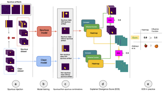
Figure 1: Explainer Divergence Score (EDS). With one engineered spurious dataset and one clean dataset, we train two separate classification models. These models evaluate different combinations of spurious and non-spurious examples. EDS can assess a post-hoc explainer’s ability to detect spurious correlations. In comparison to previous work, our approach allows us to compare the performance of different types of post-hoc explainers directly.

2 Related Work

Spurious Correlations

Spurious Correlations in DNNs have been the subject of a increasingly diverse body of work, with contributors analysing them through the lenses of distribution shift [19, 20], shortcut learning [6] and causal inference [21, 22]. Spurious correlations have raised issues in areas as diverse as privacy [23], fairness [24], and adversarial attacks [25]. Recent work has focused on identifying where spurious correlations manifest and their properties, finding they often appear in practical settings [5, 6, 26, 7, 8].

Post-Hoc Explainers

Post-hoc explainability methods generate explanations of the inference process of an arbitrary trained DNN. Numerous post-hoc explainers have been proposed.

Feature attribution methods or ‘heatmaps’ in Computer Vision domains, measure the effect of each individual input (e.g., pixel) on the output of a DNN by either leveraging input perturbation [14] or gradient information [13, 27]. Influential examples or influence function methods [28, 15] instead quantify the effect of specific training examples on a given output. Concept extraction methods [29, 16] seek to measure a DNN’s reliance on a set of understandable concepts. These methods are naturally interpretable and extendable to many DNN architectures [30, 31].

Recent work has called into question the effectiveness of post-hoc explainers in both adversarial [32, 33] and non-adversarial [34, 35, 36, 37] settings. Given these deficiencies and their widespread usage, systematic methods of comparing and evaluating post-hoc explanations have became increasingly needed.

Evaluating Explainers

There is no generally agreed method for comparing and evaluating post-hoc explainers. The majority of previous work has focused on feature attribution methods, proposing metrics to measure desirable qualities about the attribution method [38, 39, 40]. The metrics often rely on semi-synthetic datasets containing ‘ground truth’ explanations that correspond to the presence of known spurious signals [41, 42]. Metrics for other explainers remain limited with few exceptions [43], and human trials are often still the only viable approach.

The closest work to ours is Adebayo et al. [12] which formulates a paradigm for evaluating DNN explainers for the purpose of identifying spurious correlations. Similar to our work, they focus on analysing spurious correlations in settings where the spurious signal is not known ahead of time via comparing explainers from spurious and non-spurious models. However, their framework does not allow for the direct comparison between different types of explainers as their proposed quantities have different units for different types of explainers. To the best of our knowledge, this work is the only presentation of a method for evaluating a post-hoc explainer’s ability to detect spurious correlations that is comparable across all types of explainers while remaining focused on the context where the spurious signal is unknown.

3 Explainer Divergence Score

We motivate our approach by considering the setting where a user seeks to determine whether a given model depends on a spurious signal using a post-hoc explainer. They inspect an explanation generated from a model prediction and use it to predict whether the model is spurious or not. Similarly to Adebayo et al. [12], we expect a high-quality explainer to generate very different explanations from spurious models compared to non-spurious models.

This can be framed as a binary classification problem, where a classifier outputs a binary label corresponding to a prediction of a model’s dependence on a spurious signal based upon an explanation as input. The classifier under this formulation is a machine learning model that takes the place of the user, and is trained to distinguish between explanations generated by spurious models and explanations generated by non-spurious models. A visual summary of our approach can be found in Figure 1.

Critically, the classifier is trained to distinguish between explanations generated by all spurious and non-spurious models generated by a specified training strategy, instead of any individual pair. This allows the classifier to generalize to unseen models much like a human user would be expected to. We detail how we accomplish this in Section 4.1.

EDS is defined as the performance of this binary classifier in predicting model spuriousness on explanations generated using unseen models - and can be interpreted as a measure of explainer quality.

We can view our trained binary classifier’s loss as an estimate of the distance between the distribution of explanations from spurious and non-spurious models respectively. Assume we have a trained binary classifier $f_{\hat{\theta}}$ parameterized by $\theta\in\Theta$. We train this classifier by minimizing the loss $\ell$ consisting of the cross-entropy $H$ between the distribution represented by the output of the model and $Y|\mathrm{x}$, that is, the distribution $Y$ conditioned on the random variable $\mathrm{x}$ where $Y$ is the Bernoulli distribution of binary labels of a given explanation in our training set (whether the model that generated it is spurious or non-spurious) and $\mathrm{x}$ is a random variable distributed according to the mixture distribution $X$ of equally weighted explanations from both the spurious and non-spurious models. We then have:

$$\ell(f_{\hat{\theta}})= \min_{\theta\in\Theta}\mathbb{E}_{\mathrm{x}\sim X}\left[H\left(Y|\mathrm{x},f_{\theta}(\mathrm{x})\right)\right]$$ (1)

$$= 1-D_{\mathrm{JS}}(X|\mathrm{y}=0,X|\mathrm{y}=1)$$ (2)

$$\quad\quad+\min_{\theta\in\Theta}\mathbb{E}_{\mathrm{x}\sim X}\left[D_{\mathrm{KL}}\left(Y|\mathrm{x}\|f_{\theta}(\mathrm{x})\right)\right]$$ (3)

Where $D_{\mathrm{JS}}$ represents the Jensen-Shannon Divergence and $D_{\mathrm{KL}}$ represents the Kullback–Leibler Divergence, and all quantities are measured in bits of entropy. The full derivation of this expression is present in the Supplementary Material 6. Ideally, for a well trained classifier $f_{\hat{\theta}}$ of sufficient expressiveness, we would expect the distribution represented by the output of our classifier $f_{\hat{\theta}}(\mathrm{x})$ to approximate the true distribution of $Y|\mathrm{x}$, meaning the Kullback-Leibler Divergence between them is close to $0$:

$$\mathbb{E}_{\mathrm{x}\sim X}\left[D_{\mathrm{KL}}\left(Y|\mathrm{x}\|f_{\hat{\theta}}(\mathrm{x})\right)\right]\simeq 0$$ (4)

And thus:

$$\ell(f_{\hat{\theta}})\simeq 1-D_{\mathrm{JS}}(X|\mathrm{y}=0,X|\mathrm{y}=1)$$ (5)

In which case the loss of our trained model can be seen as approximating the Jensen-Shannon Divergence between the distribution of explanations generated by spurious models and the distribution of explanations generated by non-spurious models. Moreover, as all quantities share the same unit (information), they are directly comparable across explainers.

In practice, sufficient classifier accuracy for Equation 4 to hold appears to be uncommon, leading to an average loss that is unbounded above and difficult to estimate. Hence we define our EDS as the classification accuracy of the binary classifier instead. This has the added advantage of providing an interpretable baseline for our metrics - if the classifier can not do better than random guessing (EDS of 0.5), then the classifier has failed to capture any information in the explanations useful for determining model spuriousness and thus there’s a very low likelihood the explainer captures any information about the spurious signal.

4 Experiments

Using a similar setup to Adebayo et al. [12], Yang and Chaudhuri [44], we investigated three different types of spurious artifacts:

• Square - a small square in the top left corner of the image

• Stripe - a vertical stripe 9 pixels from the left of the image

• Noise - uniform Gaussian noise applied to every pixel value of the image

Examples of each spurious artifact on both the dSprites and 3dshapes datasets are present in the Supplementary Material 6.

We experiment to determine the effect of the intensity of each spurious artifact on a model’s spurious behaviour, and then trained models to maximize this spuriousness. The details of this experiment and overall model training procedure can be found in the Supplementary Material 6.

4.1 EDS Experimental Setup

For all datasets and explainers, we evaluate the Explainer Divergence Score (EDS) as follows. We split the dataset into three partitions - 80% partition used for model training, 14% partition used for binary classifier training, and 6% partition used for validation.

Recall in Section 3 we defined EDS using a binary classifier trained to distinguish between explanations generated across all spurious and non-spurious models. Training a new model for every explanation is far too computationally intensive. To rectify this for each spurious artifact we train 100 spurious and 100 non-spurious models on our model training dataset partition, using different weight initialization, and use this sample as an estimate of the complete distribution of trained spurious and non-spurious models respectively. We train models and ensure they are spurious or non-spurious respectively using the procedure detailed in the Supplementary Material 6.

We reserve 30 spurious and non-spurious models each for validation and use the remaining 70 of each set to generate training data for our binary classifier. Images from the respective dataset partition are combined with a randomly selected model to generate an explanation as well as a binary class label corresponding to whether the model came from a spurious or non-spurious set. A classifier is then trained on this data to use the explanations to predict this class label.

Finally, our remaining 30 spurious and 30 non-spurious models are combined with the validation dataset partition to generate explanations in the same fashion as in training. The label prediction accuracy of the binary classifier on this set is then our estimate of the Explainer Divergence Score of the given explainer for this spurious signal. Further experimental setup details are noted in the Supplementary Material 6.

4.2 Subclass Definitions

For all EDS results we display accuracy not just over the entire dataset (noted as ‘Overall’ in figures), but also subdivided by the task label and the presence of the spurious artifact in the image. There are four subclasses in total:

• Images from the Spurious Class without the Spurious Artifact (abbreviated as ‘S/NA’ in figures)

• Images from Non-Spurious Classes without the Spurious Artifact (abbreviated as ‘NS/NA’ in figures)

• Images from the Spurious Class with the Spurious Artifact (abbreviated as ‘S/A’ in figures)

• Images from Non-Spurious Classes with the Spurious Artifact (abbreviated as ‘NS/A’ in figures)

For example, say we had a class consisting of images of ‘circles’ and another of images of ‘squares’, and we trained a classification model between the two where we injected spurious Gaussian noise into the ‘circles’ class. ‘S/NA’ would correspond to images of circles without Gaussian noise, ‘NS/NA’ would correspond to images of squares without Gaussian noise, ‘S/A’ would correspond to images of circles with Gaussian noise, and ‘NS/A’ would correspond to images of squares with Gaussian noise.

This subdivision allows us to interpret the type of images the explainer can effectively use to determine model spuriousness. This is analogous to what is done in Adebayo et al. [12] via the ‘Cause-for-Concern Metric’ (CCM) and ‘False Alarm Metric’ (FAM) that measure results by whether the spurious artifact is present in the image, but we present results in even finer detail with added class information.

4.3 Synthetic Explainer Comparison

We compare our EDS method to the approach in Adebayo et al. [12], starting with a simple example. We consider a toy classification task with two simple classes (the dSprites classes of a ‘heart’ and ‘oval’) with the ‘stripe’ spurious artifact injected. Instead of using a specific spurious detection method, we instead construct synthetic explainers that represent the expected behaviour of each method under ideal circumstances. We construct these ‘ideal’ explainers as follows:

• Heatmaps - for the spurious model the explainer places all emphasis on the stripe for all images where it is present and the area where the stripe would be for images from the spurious class without the stripe. The explainer puts all emphasis on the shape for all cases with the non-spurious model and for the spurious model on non-spurious classes without the stripe.

• Influential Examples - for the spurious model the explainer selects influential examples of the spurious class with the stripe for all images unless it is an image from a non-spurious class without the stripe. For the non-spurious model the explainer always selects examples of the correct class with the correct presence of the spurious artifact.

• Concept Extraction - For concept extraction we specify two binary concepts, one of the class label and one of the presence of the spurious artifact. We assume the spurious model can detect both perfectly, and thus extracts both accurately. On the other hand, the non-spurious model is invariant to spurious artifact in all circumstances, and thus always extracts that it is not present.

In addition to these ideal explainers, we also create ‘noisy’ variants where we inject noise across every explanation as well as a purely random variant where the corresponding explanations consist purely of noise. For heatmaps we inject uniform Gaussian noise to the heatmap, for influential examples we specify a chance (100% in the noise variant) of randomly selecting a training image, and for concept extraction we specify a chance (100% in the noise variant) of predicting a random concept label.

We evaluate both our EDS and the KSSD, CCM and FAM metrics [12] on these examples. For these metrics we specify similarity functions as follows: for heatmaps we use the SSIM similarity function as specified in [12], for influential examples we use the Bhattacharyya coefficient [45] between the distributions of the class labels and the presence of a spurious artifact in the influential examples, and for concept extraction we use the negative of the L2 distance between concept labels as a ‘similarity’ function. The results are shown in Table 1.

Explainers	Explainer Divergence Scores					Adebayo et al. [12] Metrics
	Overall	S/NA	NS/NA	S/A	NS/A	KSSD	CCM	FAM
Heatmaps
Ideal	0.823	0.943	0.492	0.959	0.896	1.000	0.991	0.990
Noisy	0.702	0.771	0.459	0.805	0.771	0.970	0.993	0.993
Random	0.512	0.518	0.510	0.537	0.484	0.965	0.996	0.996
Influence
Ideal	0.824	0.955	0.496	0.949	0.896	1.000	0.500	0.000
Noisy	0.668	0.734	0.490	0.736	0.713	0.587	0.712	0.656
Random	0.515	0.510	0.516	0.520	0.514	0.000	0.915	0.927
Concept
Ideal	0.750	0.500	0.500	1.000	1.000	0.000	0.000	-0.500
Noisy	0.617	0.488	0.535	0.723	0.721	-0.284	-0.412	-0.514
Random	0.491	0.490	0.475	0.527	0.473	-0.494	-0.481	-0.509

Table 1: Results of evaluating EDS on the specific synthetic explainers averaged over 5 runs. We observe clear outperformance of heatmaps and influential examples over concept extraction, as well as the complete failure of the ‘random’ explainer in the EDS results. However, these are not visible in the KSSD, CCM and FAM metrics [12] results. Standard deviation estimates are provided in the Supplementary Material 6, with all results having estimated 95% confidence intervals within $\pm 0.03$.

Synthetic ‘ideal’ explainers are useful as we can specify in advance exactly how our explainers should perform between the spurious and non-spurious models in each subclass. Cases where the explanations generated from spurious and non-spurious models are drawn from the same distribution should result in the worst possible metrics. Conversely, cases where the explanations are always radically different should result in close to perfect metrics.

This is exactly what we observe with EDS. Our approach finds the ideal heatmap and influential examples almost perfectly identify model spuriousness - failing only on explanations generated from images from a non-spurious class without the spurious artifact. The ideal concept extraction explainer additionally falls short on images from the spurious class with the spurious artifact, indicating that this specification is a worse explainer for detecting spurious correlations then the competing methods.

We observe that the KSSD, CCM and FAM metrics from Adebayo et al. [12] fall short in this type of analysis: different types of explainers use different similarity functions with different units that are not comparable directly. This is a major innovation of our method over the existing state of the art.

Our method comes to our expected conclusion that the ideal explainers capture more information about model spuriousness than the noisy explainers, while the random explainers completely fail to capture any information about model spuriousness. This declining performance can also be seen in the KSSD, CCM and FAM metrics - but the utter failure of the random explainers is not visible with these metrics. With EDS, if the trained classifier fails to achieve at least 50% accuracy, we can interpret the explainer as having no information about the model’s spuriousness. This is not possible using the KSSD, CCM and FAM metrics without explicitly running a baseline for every type of explainer evaluated.

4.4 Real Explainer Comparison

To test EDS on real explainer methods, we conduct experiments on reduced versions of both the dSprites [17] and the 3dshapes [18] datasets. We train models to perform a shape classification task and arbitrarily select one class to be the spurious class for each experiment.

We chose some commonly used methods as representatives for each explainer type of interest. We use Integrated Gradients [13] as our chosen feature attribution method. For influential examples we use the TraceInCP method [15], and for concept extraction we use Concept Model Extraction (CME) [46]. Examples of each explanation on images from the dSprites dataset are present in the Supplementary Material 6.

More detailed information about the configuration setup for each experiment is present in the Supplementary Material 6.

We display results for dSprites in Table 2 and results for 3dshapes in Table 3. For comparison, we also evaluate the KSSD, CCM, and FAM metrics formulated in Adebayo et al. [12] on both dSprites and 3dshapes.

Explainers	Explainer Divergence Scores					Adebayo et al. [12] Metrics
	Overall	S/NA	NS/NA	S/A	NS/A	KSSD	CCM	FAM
Square
Heatmap	0.799	0.837	0.590	0.902	0.916	0.851	0.877	0.837
Influence	0.887	0.937	0.860	0.891	0.887	0.562	0.991	0.989
Concept	0.715	0.645	0.578	0.827	0.831	-0.062	-0.074	-0.076
Stripe
Heatmap	0.831	0.901	0.689	0.958	0.870	0.877	0.880	0.878
Influence	0.881	0.892	0.829	0.909	0.913	0.561	0.991	0.980
Concept	0.707	0.618	0.596	0.788	0.815	-0.061	-0.074	-0.077
Noise
Heatmap	0.717	0.857	0.610	0.872	0.682	0.728	0.877	0.804
Influence	0.795	0.884	0.707	0.890	0.796	0.566	0.970	0.966
Concept	0.744	0.650	0.652	0.863	0.808	-0.062	-0.078	-0.076

Table 2: Results of evaluating EDS on the dSprites dataset averaged over 5 runs. We observe the outperformance of influential examples over heatmaps and concept extraction visible in the EDS results but not in the comparative metrics. Standard deviation estimates are provided in the Supplementary Material 6., with all results having estimated 95% confidence intervals within $\pm 0.04$.

Explainers	Explainer Divergence Scores					Adebayo et al. [12] Metrics
	Overall	S/NA	NS/NA	S/A	NS/A	KSSD	CCM	FAM
Square
Heatmap	1.00	1.00	1.00	1.00	1.00	0.680	0.828	0.826
Influence	0.675	0.817	0.615	0.696	0.682	0.562	0.991	0.989
Concept	0.595	0.532	0.562	0.651	0.628	-0.156	-0.080	-0.072
Stripe
Heatmap	0.996	0.993	0.997	0.998	0.994	0.644	0.810	0.807
Influence	0.867	0.922	0.844	0.903	0.861	0.561	0.991	0.980
Concept	0.720	0.653	0.636	0.783	0.795	-0.152	-0.075	-0.070
Noise
Heatmap	0.987	1.00	0.984	0.994	0.984	0.673	0.846	0.847
Influence	0.703	0.908	0.645	0.887	0.627	0.566	0.970	0.966
Concept	0.569	0.600	0.566	0.587	0.555	-0.150	-0.074	-0.074

Table 3: Results of evaluating EDS on the 3dshapes dataset averaged over 5 runs. We observe the extreme outperformance of heatmaps over the remaining explainers visible in the EDS results but not in the comparative metrics. Standard deviation estimates are provided in the Supplementary Material 6, with all results having estimated 95% confidence intervals within $\pm 0.04$.

We observe Explainer Divergence Scores significantly above the 0.5 theoretical baseline for all explainers and spurious artifacts in both datasets. This indicates all of our explainers are successful in capturing information about the model’s spuriousness in both tasks. The key advantage of EDS over previous work is that we can now directly compare the performance of explainers for detecting model spuriousness for the specified task and spurious artifact. We interpret our results with this aim in mind.

We find the strongest performance for heatmaps and influential examples. EDS was highest for images in the spurious class without the spurious artifact, lowest for images in non-spurious classes without the spurious artifact, and somewhat high for images with the spurious artifact regardless of class. These findings appear consistent across all three of our chosen spurious artifacts, and in both datasets. We notice a sharp drop in performance for our Gaussian noise spurious artifact compared to the more localized spurious artifacts.

Concept extractions consistently perform worse than the other two explainers, operating well only on images with the explicit presence of the spurious artifact. This follows our expectations - we would expect concept extraction to more effectively identify the presence of the spurious signal concept from the activations of spurious models compared to activations of non-spurious models that have learned to become invariant to them. Moreover the dimensionality of our the concept predictions is much lower than explanations for the other two explainers, limiting their expressiveness. Interestingly while performance on images without the spurious artifact is poor, it is still above our 0.5 theoretical baseline despite there being no obvious reason for concept predictions to shift between spurious and non-spurious models. This is further discussed in Section 4.5.

We notice significant differences in explainer performance between the dSprites and 3dshapes datasets. While in dSprites we find slightly higher performance for influential examples over heatmaps, in 3dshapes we find significant strong performance for heatmaps across all experiments. In 3dshapes often our EDS binary classifier identifies the spuriousness of a given model from a heatmap with 100% accuracy. This is in sharp contrast to the other two explainers that perform worse with 3dshapes, performing only comparably using the ‘stripe’ spurious artifact. Despite this diminished performance, both influential examples and concept extraction still perform above our 0.5 theoretical baseline for EDS.

4.5 Discussion

These results favour heatmaps and influential examples, which are very effective at detecting model spuriousness in both experiments with real explainer methods. Conversely concept extraction consistently performed the worst, and is only useful on images for which the spurious artifact is present. As expected, performance is sensitive to the dataset and specified task.

We conduct further experiments to confirm Explainer Divergence Scores are robust to our choice of optimization procedure and model architecture. These are expanded upon in the Supplementary Material 6.

In both datasets, we observe EDS performances significantly above the 0.5 theoretical baseline for all explainers, spurious artifacts, and subclasses. Notably this is seen even with images from unrelated, non-spurious classes without the presence of the spurious artifact.

This has interesting implications about the utility of post-hoc explainers in detecting model spuriousness. For example, heatmaps generated from 3dshapes images in non-spurious classes without the spurious artifact do not show any obvious signal that a human could use to identify their respective model has some sort of spurious dependency. Yet a trained classifier with sufficient prior knowledge can diagnose whether the model depends upon a spurious signal with extremely high certainty. Information present in our explanations indicating spuriousness may not always be perceptible by a human observer, and identifying ways to extract or isolate this information may prove useful in designing more effective explainers.

This is particularly evident in the case of concept extraction where there is no clear hypothesis for why spurious and non-spurious models would have differing information about the underlying concepts in images from the non-spurious class without the spurious artifact. This suggests that the presence of a spurious correlation can affect a model’s ability to extract features in entirely unrelated image classes.

5 Conclusion

We present Explainer Divergence Scores - a novel method for evaluating post-hoc explainers for the purposes of detecting unknown spurious correlations.

Across three experiments we show EDS’s superior capabilities over state of the art post-hoc explainer evaluation methods. EDS provides an interpretable estimate of the amount of information an explainer can capture about a DNN’s dependence on an unknown spurious signal. Moreover EDS allows direct comparisons between different types of explainers, unlike previous methods, letting us quantitatively identify and evaluate the best explainer for a given dataset and spurious signal.

In contrast to previous work [12], our results reveal that commonly used post-hoc explainers contain substantial amount of information about a model’s dependence on unknown spurious signals. This information is often unidentifiable by human observers, and yet can be used by a well-trained classifier to detect dependencies on images seemingly unrelated to the spurious signal. Our findings suggest that future research into post-hoc explanations should focus on identifying and utilizing this unseen information.

6 Supplementary Material

Additional information about our work, including a more detailed mathematical justification, ancillary experiments, and standard error estimates for all our results are detailed in the Appendix available at this link.

References

- Chouldechova [2017] A. Chouldechova, Fair prediction with disparate impact: A study of bias in recidivism prediction instruments, Big Data 5 (2017) 153–163. URL: https://doi.org/10.1089/big.2016.0047. doi:10.1089/big.2016.0047.
- Doshi-Velez and Kim [2017] F. Doshi-Velez, B. Kim, Towards a rigorous science of interpretable machine learning, 2017. URL: https://arxiv.org/abs/1702.08608. doi:10.48550/ARXIV.1702.08608.
- Datta et al. [2015] A. Datta, M. C. Tschantz, A. Datta, Automated experiments on ad privacy settings, Proc. Priv. Enhancing Technol. 2015 (2015) 92–112. URL: https://doi.org/10.1515/popets-2015-0007. doi:10.1515/popets-2015-0007.
- Buolamwini and Gebru [2018] J. Buolamwini, T. Gebru, Gender shades: Intersectional accuracy disparities in commercial gender classification, in: S. A. Friedler, C. Wilson (Eds.), Conference on Fairness, Accountability and Transparency, FAT 2018, 23-24 February 2018, New York, NY, USA, volume 81 of Proceedings of Machine Learning Research, PMLR, 2018, pp. 77–91. URL: http://proceedings.mlr.press/v81/buolamwini18a.html.
- Lapuschkin et al. [2019] S. Lapuschkin, S. Wäldchen, A. Binder, G. Montavon, W. Samek, K. Müller, Unmasking clever hans predictors and assessing what machines really learn, CoRR abs/1902.10178 (2019). URL: http://arxiv.org/abs/1902.10178. arXiv:1902.10178.
- Geirhos et al. [2020] R. Geirhos, J. Jacobsen, C. Michaelis, R. S. Zemel, W. Brendel, M. Bethge, F. A. Wichmann, Shortcut learning in deep neural networks, Nat. Mach. Intell. 2 (2020) 665–673. URL: https://doi.org/10.1038/s42256-020-00257-z. doi:10.1038/s42256-020-00257-z.
- Sagawa et al. [2020] S. Sagawa, A. Raghunathan, P. W. Koh, P. Liang, An investigation of why overparameterization exacerbates spurious correlations, in: Proceedings of the 37th International Conference on Machine Learning, ICML 2020, 13-18 July 2020, Virtual Event, volume 119 of Proceedings of Machine Learning Research, PMLR, 2020, pp. 8346–8356. URL: http://proceedings.mlr.press/v119/sagawa20a.html.
- Mahmood et al. [2021] U. Mahmood, R. Shrestha, D. Bates, L. Mannelli, G. Corrias, Y. Erdi, C. Kanan, Detecting spurious correlations with sanity tests for artificial intelligence guided radiology systems, Frontiers in Digital Health 3 (2021). doi:10.3389/fdgth.2021.671015.
- Adebayo et al. [2020] J. Adebayo, M. Muelly, I. Liccardi, B. Kim, Debugging tests for model explanations, in: H. Larochelle, M. Ranzato, R. Hadsell, M. Balcan, H. Lin (Eds.), Advances in Neural Information Processing Systems 33: Annual Conference on Neural Information Processing Systems 2020, NeurIPS 2020, December 6-12, 2020, virtual, 2020. URL: https://proceedings.neurips.cc/paper/2020/hash/075b051ec3d22dac7b33f788da631fd4-Abstract.html.
- Han et al. [2020] X. Han, B. C. Wallace, Y. Tsvetkov, Explaining black box predictions and unveiling data artifacts through influence functions, in: D. Jurafsky, J. Chai, N. Schluter, J. R. Tetreault (Eds.), Proceedings of the 58th Annual Meeting of the Association for Computational Linguistics, ACL 2020, Online, July 5-10, 2020, Association for Computational Linguistics, 2020, pp. 5553–5563. URL: https://doi.org/10.18653/v1/2020.acl-main.492. doi:10.18653/v1/2020.acl-main.492.
- Dimanov [2021] B. Dimanov, Interpretable Deep Learning: Beyond Feature-Importance with Concept-based Explanations, Ph.D. thesis, University of Cambridge, 2021.
- Adebayo et al. [2022] J. Adebayo, M. Muelly, H. Abelson, B. Kim, Post hoc explanations may be ineffective for detecting unknown spurious correlation, in: International Conference on Learning Representations, 2022. URL: https://openreview.net/forum?id=xNOVfCCvDpM.
- Sundararajan et al. [2017] M. Sundararajan, A. Taly, Q. Yan, Axiomatic attribution for deep networks, in: D. Precup, Y. W. Teh (Eds.), Proceedings of the 34th International Conference on Machine Learning, ICML 2017, Sydney, NSW, Australia, 6-11 August 2017, volume 70 of Proceedings of Machine Learning Research, PMLR, 2017, pp. 3319–3328. URL: http://proceedings.mlr.press/v70/sundararajan17a.html.
- Ribeiro et al. [2016] M. T. Ribeiro, S. Singh, C. Guestrin, "why should I trust you?": Explaining the predictions of any classifier, in: B. Krishnapuram, M. Shah, A. J. Smola, C. C. Aggarwal, D. Shen, R. Rastogi (Eds.), Proceedings of the 22nd ACM SIGKDD International Conference on Knowledge Discovery and Data Mining, San Francisco, CA, USA, August 13-17, 2016, ACM, 2016, pp. 1135–1144. URL: https://doi.org/10.1145/2939672.2939778. doi:10.1145/2939672.2939778.
- Pruthi et al. [2020] G. Pruthi, F. Liu, S. Kale, M. Sundararajan, Estimating training data influence by tracing gradient descent, in: H. Larochelle, M. Ranzato, R. Hadsell, M. Balcan, H. Lin (Eds.), Advances in Neural Information Processing Systems 33: Annual Conference on Neural Information Processing Systems 2020, NeurIPS 2020, December 6-12, 2020, virtual, 2020. URL: https://proceedings.neurips.cc/paper/2020/hash/e6385d39ec9394f2f3a354d9d2b88eec-Abstract.html.
- Kazhdan et al. [2020] D. Kazhdan, B. Dimanov, M. Jamnik, P. Liò, A. Weller, Now you see me (CME): concept-based model extraction, in: S. Conrad, I. Tiddi (Eds.), Proceedings of the CIKM 2020 Workshops co-located with 29th ACM International Conference on Information and Knowledge Management (CIKM 2020), Galway, Ireland, October 19-23, 2020, volume 2699 of CEUR Workshop Proceedings, CEUR-WS.org, 2020. URL: http://ceur-ws.org/Vol-2699/paper02.pdf.
- Matthey et al. [2017] L. Matthey, I. Higgins, D. Hassabis, A. Lerchner, dsprites: Disentanglement testing sprites dataset, https://github.com/deepmind/dsprites-dataset/, 2017.
- Burgess and Kim [2018] C. Burgess, H. Kim, 3d shapes dataset, https://github.com/deepmind/3dshapes-dataset/, 2018.
- Zhou et al. [2021] C. Zhou, X. Ma, P. Michel, G. Neubig, Examining and combating spurious features under distribution shift, in: M. Meila, T. Zhang (Eds.), Proceedings of the 38th International Conference on Machine Learning, ICML 2021, 18-24 July 2021, Virtual Event, volume 139 of Proceedings of Machine Learning Research, PMLR, 2021, pp. 12857–12867. URL: http://proceedings.mlr.press/v139/zhou21g.html.
- Sagawa et al. [2020] S. Sagawa, P. W. Koh, T. B. Hashimoto, P. Liang, Distributionally robust neural networks, in: 8th International Conference on Learning Representations, ICLR 2020, Addis Ababa, Ethiopia, April 26-30, 2020, OpenReview.net, 2020. URL: https://openreview.net/forum?id=ryxGuJrFvS.
- Arjovsky et al. [2019] M. Arjovsky, L. Bottou, I. Gulrajani, D. Lopez-Paz, Invariant risk minimization, CoRR abs/1907.02893 (2019). URL: http://arxiv.org/abs/1907.02893. arXiv:1907.02893.
- Moneda [2021] L. Moneda, Spurious correlation machine learning and causality, Blogpost at lgmoneda.github.io (2021).
- Leino and Fredrikson [2020] K. Leino, M. Fredrikson, Stolen memories: Leveraging model memorization for calibrated white-box membership inference, in: S. Capkun, F. Roesner (Eds.), 29th USENIX Security Symposium, USENIX Security 2020, August 12-14, 2020, USENIX Association, 2020, pp. 1605–1622. URL: https://www.usenix.org/conference/usenixsecurity20/presentation/leino.
- Mehrabi et al. [2021] N. Mehrabi, F. Morstatter, N. Saxena, K. Lerman, A. Galstyan, A survey on bias and fairness in machine learning, ACM Comput. Surv. 54 (2021) 115:1–115:35. URL: https://doi.org/10.1145/3457607. doi:10.1145/3457607.
- Chen et al. [2017] X. Chen, C. Liu, B. Li, K. Lu, D. Song, Targeted backdoor attacks on deep learning systems using data poisoning, CoRR abs/1712.05526 (2017). URL: http://arxiv.org/abs/1712.05526. arXiv:1712.05526.
- Xiao et al. [2021] K. Y. Xiao, L. Engstrom, A. Ilyas, A. Madry, Noise or signal: The role of image backgrounds in object recognition, in: 9th International Conference on Learning Representations, ICLR 2021, Virtual Event, Austria, May 3-7, 2021, OpenReview.net, 2021. URL: https://openreview.net/forum?id=gl3D-xY7wLq.
- Selvaraju et al. [2016] R. R. Selvaraju, A. Das, R. Vedantam, M. Cogswell, D. Parikh, D. Batra, Grad-cam: Why did you say that? visual explanations from deep networks via gradient-based localization, CoRR abs/1610.02391 (2016). URL: http://arxiv.org/abs/1610.02391. arXiv:1610.02391.
- Koh and Liang [2017] P. W. Koh, P. Liang, Understanding black-box predictions via influence functions, in: D. Precup, Y. W. Teh (Eds.), Proceedings of the 34th International Conference on Machine Learning, ICML 2017, Sydney, NSW, Australia, 6-11 August 2017, volume 70 of Proceedings of Machine Learning Research, PMLR, 2017, pp. 1885–1894. URL: http://proceedings.mlr.press/v70/koh17a.html.
- Kim et al. [2018] B. Kim, M. Wattenberg, J. Gilmer, C. J. Cai, J. Wexler, F. B. Viégas, R. Sayres, Interpretability beyond feature attribution: Quantitative testing with concept activation vectors (TCAV), in: J. G. Dy, A. Krause (Eds.), Proceedings of the 35th International Conference on Machine Learning, ICML 2018, Stockholmsmässan, Stockholm, Sweden, July 10-15, 2018, volume 80 of Proceedings of Machine Learning Research, PMLR, 2018, pp. 2673–2682. URL: http://proceedings.mlr.press/v80/kim18d.html.
- Kazhdan et al. [2020] D. Kazhdan, B. Dimanov, M. Jamnik, P. Liò, MEME: generating RNN model explanations via model extraction, CoRR abs/2012.06954 (2020). URL: https://arxiv.org/abs/2012.06954. arXiv:2012.06954.
- Magister et al. [2021] L. C. Magister, D. Kazhdan, V. Singh, P. Liò, Gcexplainer: Human-in-the-loop concept-based explanations for graph neural networks, CoRR abs/2107.11889 (2021). URL: https://arxiv.org/abs/2107.11889. arXiv:2107.11889.
- Kindermans et al. [2019] P. Kindermans, S. Hooker, J. Adebayo, M. Alber, K. T. Schütt, S. Dähne, D. Erhan, B. Kim, The (un)reliability of saliency methods, in: W. Samek, G. Montavon, A. Vedaldi, L. K. Hansen, K. Müller (Eds.), Explainable AI: Interpreting, Explaining and Visualizing Deep Learning, volume 11700 of Lecture Notes in Computer Science, Springer, 2019, pp. 267–280. URL: https://doi.org/10.1007/978-3-030-28954-6_14. doi:10.1007/978-3-030-28954-6_14.
- Dimanov et al. [2020] B. Dimanov, U. Bhatt, M. Jamnik, A. Weller, You shouldn’t trust me: Learning models which conceal unfairness from multiple explanation methods, in: H. Espinoza, J. Hernández-Orallo, X. C. Chen, S. S. ÓhÉigeartaigh, X. Huang, M. Castillo-Effen, R. Mallah, J. A. McDermid (Eds.), Proceedings of the Workshop on Artificial Intelligence Safety, co-located with 34th AAAI Conference on Artificial Intelligence, SafeAI@AAAI 2020, New York City, NY, USA, February 7, 2020, volume 2560 of CEUR Workshop Proceedings, CEUR-WS.org, 2020, pp. 63–73. URL: http://ceur-ws.org/Vol-2560/paper8.pdf.
- Ghorbani et al. [2017] A. Ghorbani, A. Abid, J. Y. Zou, Interpretation of neural networks is fragile, CoRR abs/1710.10547 (2017). URL: http://arxiv.org/abs/1710.10547. arXiv:1710.10547.
- Basu et al. [2021] S. Basu, P. Pope, S. Feizi, Influence functions in deep learning are fragile, in: 9th International Conference on Learning Representations, ICLR 2021, Virtual Event, Austria, May 3-7, 2021, OpenReview.net, 2021. URL: https://openreview.net/forum?id=xHKVVHGDOEk.
- Locatello et al. [2019] F. Locatello, S. Bauer, M. Lucic, G. Rätsch, S. Gelly, B. Schölkopf, O. Bachem, Challenging common assumptions in the unsupervised learning of disentangled representations, in: Reproducibility in Machine Learning, ICLR 2019 Workshop, New Orleans, Louisiana, United States, May 6, 2019, OpenReview.net, 2019. URL: https://openreview.net/forum?id=Byg6VhUp8V.
- Zhou et al. [2022] Y. Zhou, S. Booth, M. T. Ribeiro, J. Shah, Do feature attribution methods correctly attribute features?, in: Thirty-Sixth AAAI Conference on Artificial Intelligence, AAAI 2022, Thirty-Fourth Conference on Innovative Applications of Artificial Intelligence, IAAI 2022, The Twelveth Symposium on Educational Advances in Artificial Intelligence, EAAI 2022 Virtual Event, February 22 - March 1, 2022, AAAI Press, 2022, pp. 9623–9633. URL: https://ojs.aaai.org/index.php/AAAI/article/view/21196.
- Alvarez-Melis and Jaakkola [2018] D. Alvarez-Melis, T. S. Jaakkola, On the robustness of interpretability methods, CoRR abs/1806.08049 (2018). URL: http://arxiv.org/abs/1806.08049. arXiv:1806.08049.
- Dai et al. [2022] J. Dai, S. Upadhyay, U. Aïvodji, S. H. Bach, H. Lakkaraju, Fairness via explanation quality: Evaluating disparities in the quality of post hoc explanations, in: V. Conitzer, J. Tasioulas, M. Scheutz, R. Calo, M. Mara, A. Zimmermann (Eds.), AIES ’22: AAAI/ACM Conference on AI, Ethics, and Society, Oxford, United Kingdom, May 19 - 21, 2021, ACM, 2022, pp. 203–214. URL: https://doi.org/10.1145/3514094.3534159. doi:10.1145/3514094.3534159.
- Zhou et al. [2021] J. Zhou, A. H. Gandomi, F. Chen, A. Holzinger, Evaluating the quality of machine learning explanations: A survey on methods and metrics, Electronics 10 (2021). URL: https://www.mdpi.com/2079-9292/10/5/593. doi:10.3390/electronics10050593.
- Agarwal et al. [2022] C. Agarwal, E. Saxena, S. Krishna, M. Pawelczyk, N. Johnson, I. Puri, M. Zitnik, H. Lakkaraju, Openxai: Towards a transparent evaluation of model explanations, CoRR abs/2206.11104 (2022). URL: https://doi.org/10.48550/arXiv.2206.11104. doi:10.48550/arXiv.2206.11104. arXiv:2206.11104.
- Liu et al. [2021] Y. Liu, S. Khandagale, C. White, W. Neiswanger, Synthetic benchmarks for scientific research in explainable machine learning, in: J. Vanschoren, S. Yeung (Eds.), Proceedings of the Neural Information Processing Systems Track on Datasets and Benchmarks 1, NeurIPS Datasets and Benchmarks 2021, December 2021, virtual, 2021. URL: https://datasets-benchmarks-proceedings.neurips.cc/paper/2021/hash/c16a5320fa475530d9583c34fd356ef5-Abstract-round2.html.
- Zarlenga et al. [2022] M. E. Zarlenga, P. Barbiero, Z. Shams, D. Kazhdan, U. Bhatt, M. Jamnik, On the quality assurance of concept-based representations, 2022. URL: https://openreview.net/forum?id=Ehhk6jyas6v.
- Yang and Chaudhuri [2022] Y. Yang, K. Chaudhuri, Understanding rare spurious correlations in neural networks, CoRR abs/2202.05189 (2022). URL: https://arxiv.org/abs/2202.05189. arXiv:2202.05189.
- Kailath [1967] T. Kailath, The divergence and bhattacharyya distance measures in signal selection, IEEE Transactions on Communication Technology 15 (1967) 52–60. doi:10.1109/TCOM.1967.1089532.
- Kazhdan et al. [2020] D. Kazhdan, B. Dimanov, M. Jamnik, P. Liò, A. Weller, Now you see me (CME): concept-based model extraction, in: S. Conrad, I. Tiddi (Eds.), Proceedings of the CIKM 2020 Workshops co-located with 29th ACM International Conference on Information and Knowledge Management (CIKM 2020), Galway, Ireland, October 19-23, 2020, volume 2699 of CEUR Workshop Proceedings, CEUR-WS.org, 2020. URL: http://ceur-ws.org/Vol-2699/paper02.pdf.