Credit Default Swaps and the mixed-fractional CEV model

Abstract

This paper explores the capabilities of the Constant Elasticity of Variance model driven by a mixed-fractional Brownian motion (mfCEV) [araneda2020fractional] to address default-related financial problems, particularly the pricing of Credit Default Swaps. The increase in both, the probability of default and the CDS spreads under mixed-fractional diffusion compared to the standard Brownian case, improves the lower empirical performance of the standard Constant Elasticity of Variance model (CEV), yielding a more realistic model for credit events.

Keywords: Fractional Brownian motion; First-passage time; CEV model; Credit Default Swaps; Equity Default Swaps.

This version: March 14, 2024

1 Introduction

Credit Default Swaps (CDS) are derivatives designed to hedge default in the firm’s obligations, taking as reference some debt instrument (e.g., bonds). It acts as insurance since the ‘protection buyer’ is compensated (usually with the debt face value) in case of a credit default event in exchange for periodic payments to the ‘protection seller’. On the other hand, when the reference asset is just equity (stock price), and the triggering event is some pre-specified price-level barrier (namely, 30% or 50% of the initial value), we are in front of an Equity Default Swap (EDS), a deep out-of-the-money digital knock-in put option, where the option premium, instead of paid at the inception, is divided into legs along the contract duration to mimic the CDS structure. In the case of a firm’s debt default, the stock price would be worth zero or very near to the zero level, then CDS are equivalent to a zero-barrier EDS [2].

From the price modelling perspective, the geometric Brownian motion, the basic assumption of the seminal work of Black and Scholes [3], precludes hitting the zero price level and becoming ineligible to address default-related problems. In that sense, the constant elasticity of variance (CEV model) [4, 5] emerges as a candidate for this task due to some desirable properties. First, the origin is an attainable and absorbing boundary via diffusion to zero, and consequently, it includes the bankruptcy possibility. Second, the CEV model addresses some empirical facts observed in equity markets: the leverage effect, heteroskedasticity, and the implied volatility skew.

The standard CEV assumption has already been applied to credit risk pricing [7, 8]. However, the lower CDS spreads under the standard CEV model compared to the actual market data [9, 2], yields to consider some extensions as the addition of a Heston-type stochastic volatility feature to the CEV stock price [10], or the inclusion of a killing jump rate [11, 9, 2].

In this note, we want to enrich the CEV-CDS literature, including a non-standard diffusion mechanism for the CEV model, particularly the mixed-fractional Brownian motion (mfBm) which provides to the CEV model the capacity to address the long-range dependence empirical observation without sacrificing the martingale property and a better fit with market option prices [1, 12].

2 The mixed-fractional CEV model

The mfCEV establishes the following stochastic differential equation for the evolution of the asset price $S$ [1]:

$$\mathrm{d}S_{t}=rS_{t}\mathrm{d}t+\delta S_{t}^{\frac{\alpha}{2}}\mathrm{d}M_{t}^{H,\beta}$$ (1)

where $M_{t}^{H}$ is a mfBm defined as:

$$M_{t}^{H,\beta}=B_{t}+\beta B_{t}^{H}$$ (2)

being $\beta\in\mathbb{R}_{0}^{+}$, $B_{t}^{H}$ a fractional Brownian motion with Hurst parameter $\frac{3}{4}<H<1$, and $B_{t}$ an independent $\&$ standard Bm. These conditions guarantee that the mfBm is a local-martingale equivalent in law to a standard Brownian motion [13]. The parameter $\alpha$ is restricted to less than 2 in order to ensure three features: i) zero is an attainable and absorbing boundary (cf. footnote 1); ii) inverse relationship between price and volatility (Leverage effect); and iii) arbitrage-free (which is possible because $M_{t}^{H,\beta}$ is semi-martingale for $H>3/4$; see [6, 14] about the CEV model and arbitrage possibilities). The other two parameters of the model, $r$ and $\delta$, are assumed non-negative and strictly positive, respectively. The former represents the constant risk-free interest rate while the latter adjusts the at-the-money volatility level and is usually parametrized as $\delta^{2}=\sigma_{0}^{2}S_{0}^{2-\alpha}$, so $\sigma_{0}$ acts as the volatility scale parameter of the local volatility function; i.e., $\sigma\left(S,0\right)=\sigma_{0}$.

Defining the new variable $x_{t}=S_{t}^{2-\alpha}$, the related Wick-Itô calculus (Appendix A) yields to :

$$\text{d}x_{t} = \left(2-\alpha\right)\left[rx_{t}+\sigma^{2}\left(1-\alpha\right)\left(\frac{1}{2}+\beta^{2}Ht^{2H-1}\right)\right]\text{d}t+\left(2-\alpha\right)\sigma\sqrt{x_{t}}\text{d}M_{t}^{H,\beta}$$

and the corresponding transition density probability function $P=P\left(\left.x_{t},t\right|x_{0},0\right)$ obeys (c.f. Appendix B):

$$\frac{\partial P}{\partial t}=-\frac{\partial}{\partial x_{t}}\left\{\left[Ax_{t}+B\left(t\right)\right]P\right\}+C\left(t\right)\frac{\partial^{2}}{\partial x_{t}^{2}}\left[xP\right]$$ (3)

with $A=\left(2-\alpha\right)r,$ $B\left(t\right)=\sigma^{2}\left(1-\alpha\right)\left(2-\alpha\right)\left(\frac{1}{2}+\beta^{2}Ht^{2H-1}\right)$, and $C\left(t\right)=\sigma^{2}\left(2-\alpha\right)^{2}\left(\frac{1}{2}+\beta^{2}Ht^{2H-1}\right)$.

Eq. (3) is equivalent to the Fokker-Planck equation for a time-inhomogeneous Feller (square-root) process, and given the ratio $\theta=B(t)/C(t)=\left(1-\alpha\right)/\left(2-\alpha\right)<1$ is time-independent, it could be solved analytically [1, 15]. Moreover, considering these conditions, the density $g$ of the random variable $\tau=\inf\left\{t>0:x_{t}=0\right\}$ which describes first-passage time (FPT) through the zero state is given by [15]:

$$g\left(\left.0,t\right|x_{0},0\right) = \frac{1}{\Gamma\left(1-\xi\right)}\frac{\sigma^{2}\left(2-\alpha\right)^{2}\text{e}^{-\left(2-\alpha\right)rt}}{\phi\left(t\right)}\left[\frac{x_{0}}{\phi\left(t\right)}\right]^{1-\xi}\exp\left[-\frac{x_{0}}{\phi\left(t\right)}\right]$$ (4)

$$= -\frac{1}{\Gamma\left(1-\xi\right)}\frac{\partial}{\partial t}\gamma\left(1-\xi,{\displaystyle\frac{x_{0}}{\phi\left(t\right)}}\right)$$

being $\gamma\left(\bullet,\bullet\right)$ the lower incomplete gamma function, and

$$\phi\left(t\right)=\int_{0}^{t}C\left(\tilde{t}\right)\text{e}^{-\left(2-\alpha\right)r\tilde{t}}\text{d}\tilde{t}=\frac{\sigma^{2}\left(2-\alpha\right)}{2r}\left[1-\text{e}^{-\left(2-\alpha\right)rt}\right]\\ +\beta^{2}\frac{\sigma^{2}\left(2-\alpha\right)^{2}}{2\left(2H+1\right)}\text{e}^{-\left(2-\alpha\right)rt}t^{2H}\left\{2H+1+\text{e}^{\frac{1}{2}\left(2-\alpha\right)rt}\left[\left(2-\alpha\right)rt\right]^{-H}M_{H,H+1/2}\left[\left(2-\alpha\right)rt\right]\right\}$$

with $M_{\kappa,\upsilon}\left(l\right)$ the M-Whittaker function.

Thus, the first-passage-time (FPT) probability ($Q$) is equal to [15]:

$$Q\left(\left.\tau\leq t\right|x_{0},0\right)=1-\frac{\gamma\left(1-\xi,\frac{x_{0}}{\phi\left(t\right)}\right)}{\Gamma\left(1-\xi\right)}=\frac{\Gamma\left(1-\xi,{\displaystyle\frac{x_{0}}{\phi\left(t\right)}}\right)}{\Gamma\left(1-\xi\right)}$$

where $\Gamma\left(\bullet,\bullet\right)$ denotes the upper incomplete gamma function, and in consequence, the risk-neutral default probability for the mfCEV model is expressed as:

$$Q\left(\left.\tau\leq t\right|S_{0},0\right)=\frac{\Gamma\left(1-\xi,{\displaystyle\frac{S_{0}^{2-\alpha}}{\phi\left(t\right)}}\right)}{\Gamma\left(1-\xi\right)}$$

Fig. 1 plots the FPT probability through the zero state as a function of time for the mixed-fractional CEV model under different elasticity parameters: $\alpha=-2$ (blue, 1a) and $\alpha=$0 (red, 1b). Moreover, to visualize the mfCEV model sensitivity to both the Hurst exponent and $\beta$, we use $H=\left\{0.8,0.9\right\}$ and $\beta=\left\{0,1/2,1\right\}$. The case $\beta=0$ corresponds to the standard CEV specification. We have set the initial volatility $(\sigma_{0})$ at 20%, and the risk-free rate equals 5%. We see the mixed-fractional diffusion increases the default probability (as a function of both $\beta$ and $H$) compared to the classical CEV. The increment in the FPT is faster for a greater $\alpha$ at long times. Nevertheless, for short maturities, the increment is more pronounced under lower $\alpha$.

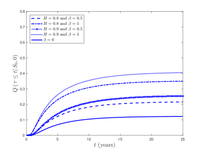
(a) CEV

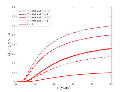
(b) $\alpha=0$ and $\sigma_{0}=20\%$

Figure 1: Probability of default (price equal to zero) under both CEV and mfCEV models, setting $S_{0}=50$, $\sigma_{0}=20\%$ and $r=5\%$.

3 CDS rates

The objective here is to compute both i) the present value ($V$) of the protection payment to the buyer due to the triggering event (100%-drop in the price level) and ii) the swap rate. For a maturity $T$, a constant risk-free rate $r$, a notional amount of 1$, and a fixed recovery rate $R$, the risk-neutral valuation yields:

$$V=\left(1-R\right)\cdot\mathbb{E}\left(\text{e}^{-r\tau}\mathbbm{1}_{\tau<T}\right)$$

where the indicator function $\mathbbm{1}_{\tau<T}$ maps a price default event in the time-interval $[0,T]$. Then,

$$V = \left(1-R\right)\int_{0}^{T}\text{e}^{-rt}g\left(\left.0,t\right|x_{0},0\right)\text{d}t$$ (5)

$$= \left(1-R\right)\left[\text{e}^{-rT}Q\left(\left.\tau\leq t\right|S_{0},0\right)+r\int_{0}^{T}\text{e}^{-rt}Q\left(\left.\tau\leq t\right|S_{0},0\right)\right]$$

On the other hand, in CDS contracts, the protection payment is divided in installments from the inception time up to either the trigger event or the expiration time, whichever comes first. Then, ignoring any accrual payment after the default, the equilibrium swap rate (coupon $C$) under typical conditions (semiannual installments and a maturity equal to an integer number of years) is given by:

$$C={\displaystyle\frac{V}{{\displaystyle\sum_{i=1}^{2T}}\text{e}^{-r\frac{i}{2}}\mathbb{E}\left[\mathbbm{1}_{\tau>\frac{i}{2}}\right]}=}{\displaystyle\frac{V}{{\displaystyle\sum_{i=1}^{2T}}\text{e}^{-r\frac{i}{2}}\left[1-Q\left(\left.\tau\leq\frac{i}{2}\right|S_{0},0\right)\right]}}$$

Table (1) shows the CDS spreads, i.e., the annual coupon payments (in basis points), when the underlying asset follows a mfCEV ($\beta=\left\{0.5,1\right\}$, $H=\left\{0.8,0.9\right\}$) and a standard CEV ($\beta=0$), with $\sigma_{0}=20\%$, $r=5\%$, a recovery rate of 50%, $\alpha=\left\{0,-2\right\}$; under different maturities, being $V$ computed by numerical integration of Eq. (5). The results confirm the dependence on both maturity and elasticity; and the lower swap rate for the classical CEV for low maturities, due to the low default probability under the standard Brownian diffusion. Meanwhile, the mfCEV provides larger coupon values, even at low tenors, as a function of both $H$ and $\beta$, allowing a flexible calibration to match the term structure of CDS spreads.

		$T=1$		$T=2$		$T=5$		$T=10$
		$\alpha=0$	$\alpha=-2$	$\alpha=0$	$\alpha=-2$	$\alpha=0$	$\alpha=-2$	$\alpha=0$	$\alpha=-2$
$\beta=0$		0.0015	14.6761	0.4976	49.3693	11.0929	71.0707	22.0907	58.1472
$\beta=0$.5	$H=0.8$	0.0220	33.0638	3.6859	97.5923	45.8409	130.6805	73.6537	107.2735
	$H=0.9$	0.0219	32.9327	4.5121	104.3824	61.1677	148.0252	99.5110	125.2780
$\beta=1$	$H=0.8$	1.3802	121.9533	45.2696	250.5198	182.4174	265.8567	206.8295	206.2857
	$H=0.9$	1.3665	121.0740	58.1627	275.5237	240.6370	307.8064	270.6823	244.4577

Table 1: CDS spread under both standard and mixed-fractional CEV model

Appendix A Itô-Wick formula for mfBm

From Eq. (2), we have that:

$$\mathbb{E}\left[\left(M_{t}^{H,\beta}\right)^{2}\right]=t+\beta^{2}t^{2H}$$

Given that the variance is bounded, for $f=f\left(t,x\left(M_{t}^{H,\beta}\right)\right)\in C^{1,2}\left(\left(0,\infty\right)\times\mathbb{R}\right)$ we have [16]:

$$\text{d}f = \frac{\partial f}{\partial t}\text{d}t+\frac{\partial f}{\partial x}\text{d}M_{t}^{H,\beta}+\frac{1}{2}\text{d}\left(t+\beta^{2}t^{2H}\right)\frac{\partial^{2}f}{\partial x^{2}}$$ (6)

$$=\frac{\partial f}{\partial t}\text{d}t+\frac{\partial f}{\partial x}\text{d}M_{t}^{H,\beta}+\frac{1}{2}\left(1+2H\beta^{2}t^{2H-1}\right)\text{d}t\frac{\partial^{2}f}{\partial x^{2}}$$

$$=\left[\frac{\partial f}{\text{$\partial t$}}+\left(\frac{1}{2}+H\beta^{2}t^{2H-1}\right)\frac{\partial^{2}f}{\text{$\partial x^{2}$}}\right]\text{d}t+\frac{\partial f}{\text{$\partial x$}}\text{d}M_{t}^{H,\beta}$$

Appendix B Effective Fokker-Planck equation

Let $y_{t}$ a stochastic process described by the following stochastic differential equation (SDE) driven by a mfBm:

$$\text{d}y_{t}=\mu\left(y_{t},t\right)\text{d}t+\sigma\left(y_{t},t\right)\text{d}M_{t}^{H,\beta}$$ (7)

then, the transformation $g=g\left(y_{t},t\right)\in C^{2}\left(\mathbb{R}\right)$ follows:

$$\text{d}g\left(y_{t}\right)=\left[\left(\frac{\partial g}{\text{$\partial y$}}\right)\mu+\left(\frac{1}{2}+H\beta^{2}t^{2H-1}\right)\sigma^{2}\frac{\partial^{2}g}{\text{$\partial y^{2}$}}\right]\text{d}t+\left(\frac{\partial g}{\text{$\partial y$}}\right)\sigma\text{d}M_{t}^{H,a,b}$$ (8)

Taking expectations at both sides of Eq. (8) and using that $\mathbb{E}\left[g\left(y_{t},t\right)\right]=\int g\cdot P\left(y_{t},t\right)$, where $P=P\left(y_{t},t\right)$ is the transition density of the random variable $y$ at time $t$; we got:

$$\int_{-\infty}^{\infty}g\frac{\partial P}{\partial t}\text{d}y=\int_{-\infty}^{\infty}\left[\left(\frac{\partial g}{\text{$\partial y$}}\right)\mu+\left(\frac{1}{2}+H\beta^{2}t^{2H-1}\right)\sigma^{2}\frac{\partial^{2}g}{\text{$\partial y^{2}$}}\right]P\text{d}y$$ (9)

Taking in account that $\int_{-\infty}^{\infty}\left(\frac{\partial g}{\text{$\partial y$}}\right)\mu P\text{d}y=-\int_{-\infty}^{\infty}g\frac{\partial\left(\mu P\right)}{\partial y}\text{d}y$ and $\int_{-\infty}^{\infty}\sigma^{2}\frac{\partial^{2}g}{\text{$\partial y^{2}$}}P\text{d}y=-\int_{-\infty}^{\infty}g\frac{\partial^{2}\left(\sigma^{2}P\right)}{\partial y^{2}}\text{d}y$, the transition density for the variable $y_{t}$ described by Eq. (7) is ruled by:

$$\frac{\partial P}{\text{$\partial t$}}=-\frac{\partial\left(\mu P\right)}{\partial y}+\left(\frac{1}{2}+H\beta^{2}t^{2H-1}\right)\frac{\partial^{2}\left(\sigma^{2}P\right)}{\partial y^{2}}$$ (10)

References

- Araneda [2020] Axel A. Araneda. The fractional and mixed-fractional CEV model. Journal of Computational and Applied Mathematics, 363:106–123, 2020.
- Mendoza-Arriaga and Linetsky [2011] Rafael Mendoza-Arriaga and Vadim Linetsky. Pricing equity default swaps under the jump-to-default extended CEV model. Finance and Stochastics, 15(3):513–540, 2011.
- Black and Scholes [1973] Fischer Black and Myron Scholes. The pricing of options and corporate liabilities. Journal of Political Economy, 81(3):637–654, 1973.
- Cox [1975.] John C. Cox. Notes on option pricing I: Constant elasticity of variance diffusions. Working paper, Stanford University, 1975.
- Cox [1996] John C. Cox. The constant elasticity of variance option pricing model. The Journal of Portfolio Management, 23(5):15–17, 1996.
- Lindsay and Brecher [2012] A. E. Lindsay and D. R. Brecher. Simulation of the CEV process and the local martingale property. Mathematics and Computers in Simulation, 82(5):868–878, 2012.
- Campi and Sbuelz [2005] Luciano Campi and Alessandro Sbuelz. Closed-form pricing of benchmark equity default swaps under the CEV assumption. Risk Letters, 1(3), 2005.
- Albanese and Chen [2005] Claudio Albanese and Oliver Chen. Pricing equity default swaps. Risk, 18(6):83, 2005.
- Carr and Linetsky [2006] Peter Carr and Vadim Linetsky. A jump to default extended CEV model: an application of Bessel processes. Finance and Stochastics, 10(3):303–330, 2006.
- Atlan and Leblanc [2005] Marc Atlan and Boris Leblanc. Hybrid equity-credit modelling. Risk, 8(8):18, 2005.
- Campi et al. [2009] Luciano Campi, Simon Polbennikov, and Alessandro Sbuelz. Systematic equity-based credit risk: A CEV model with jump to default. Journal of Economic Dynamics and Control, 33(1):93–108, 2009.
- Araneda and Bertschinger [2021] Axel A. Araneda and Nils Bertschinger. The sub-fractional CEV model. Physica A: Statistical Mechanics and its Applications, 573:125974, 2021.
- Cheridito [2001] Patrick Cheridito. Mixed fractional Brownian motion. Bernoulli, 7(6):913–934, 2001.
- Delbaen and Shirakawa [2002] Freddy Delbaen and Hiroshi Shirakawa. A note on option pricing for the constant elasticity of variance model. Asia-Pacific Financial Markets, 9(2):85–99, 2002.
- Giorno and Nobile [2021] Virginia Giorno and Amelia G. Nobile. Time-inhomogeneous Feller-type diffusion process with absorbing boundary condition. Journal of Statistical Physics, 183(3):1–27, 2021.
- Nualart and Taqqu [2008] David Nualart and Murad Taqqu. Wick–Itô formula for regular processes and applications to the Black and Scholes formula. Stochastics: An International Journal of Probability and Stochastic Processes, 80(5):477–487, 2008.