Robust Real-Time Tracking of Axis-Symmetric Magnets via Neural Networks

Abstract

Traditional tracking of magnetic markers leads to high computational costs due to the requirement for iterative optimization procedures. Furthermore, such approaches rely on the magnetic dipole model for the optimization function, leading to inaccurate results anytime a non-spherical magnet gets close to a sensor in the array. We propose to overcome these limitations by using neural networks to infer the marker’s position and orientation. Our method can obtain the magnet’s five degrees of freedom (5 DoF) in a single inference step without relying on an initial estimation. As a counterpart, the supervised training phase is data intensive. We solve this by generating synthetic, yet realistic, data via Finite Element Methods simulations. A fast and accurate inference largely compensates for the offline training preparation. We evaluate our system using different cylindrical magnets, tracked with a square array of 16 sensors. We use a portable, neural networks-oriented single-board computer for the sensors’ reading and the position inference, making our setup very compact. We compared our tracking outputs with vision-based ground truth data. Our prototype implementation tracks $5$ DoF with an averaged positional error of $4$ mm and orientation error of $8$ deg within a $0.2x0.2x0.15$ m working volume.

Keywords Passive magnet localization  $\cdot$ machine learning  $\cdot$ position and orientation tracking  $\cdot$ permanent magnets

1 Introduction

Alarge variety of applications rely on the tracking of three dimensional position and orientation. Such as decoding gesture input and providing force feedback on fingertips or tools [1, 2, 3, 4, 5] via magnetic tracking. Tracking and guiding medical instruments, such as capsules and catheters [6, 7, 8, 9, 10] also rely on magnetic markers. This widespread interest is partially driven by the fact that magnetic signals can permeate through a large variety of materials, including human tissues, without disturbance or occlusion. In addition, these systems can also benefit from comparatively affordable and more lightweight instrumentation, both in the tracker sensors and the markers.

Existing work distincts between active and passive magnetic markers. Active markers can benefit from a higher signal-to-noise ratio by allowing frequency filtering. However, tracking active emitters requires either a wired connection to the tracked object or a battery-powered circuitry [3, 11]. In contrast, Passive magnetic localization is simpler - it only requires the target to be instrumented with a permanent magnet, eliminating any need for tethered connections or active electronics on the moving elements [5, 12, 13]. Interestingly, [14] has proposed a third group of semi-passive markers. Although the tracked elements are passive, they respond with a resonant signal when excited by the nearby source. Although our work focuses on passive magnetic localization, due to its simplicity and robustness, future work could apply to many of the ideas deployed here to these other types of magnetic markers.

A vital part of the system is the algorithm that transforms magnetic signals into the marker’s 5-degree-of-freedom (5DoF) position and orientation. One common solution is to minimize the difference between a mathematical magnetic field model and the sensors’ readings. For this purpose, several non-linear optimization algorithms have been proposed and tested [15, 16]. In [13], the authors implemented an analytical computation of gradients to accelerate the optimization process. In [17], the proposed algorithm uncouples the marker’s orientation from its position, which improves the calculation speed and provides guarantees in terms of the global minima. Nonetheless, these iterative approaches come with significant challenges. First, gradient-descent algorithms are computationally expensive, which results in a trade-off between tracking precision and frequency. Second, an iterative non-convex optimization may also suffer from the non-uniqueness of the solution, converging to local minima. These challenges result in such methods being strongly dependent on their initialization.

Other approaches have explored ways to reduce the problem complexity to a linear variant, ensuring increased convergence speed and global optimality of the solution. The most drastic simplification is to directly interpolate the intensity of the reading within the sensors’ array. In [18, 19], the authors use this approach to track a stylus and a gaming object in a two-dimensional plane. In a more sophisticated configuration (cf., [20, 3, 4]) multiple sensors with known spatial arrangements give an over-constrained system of equations so that there is a unique solution to the state of a magnet. These triangulation methods are fast, however, less robust to the noise of sensors and restricted to only the positional DoFs.

Crucially, any methods’ effectiveness depends on the magnetic model’s validity. Most, if not all, of the above methods, used the first term of the multi-pole series expansion derived from Maxwell’s equations. The magnetic dipole approximation assumes any magnet to be spherical. On the one hand, this approximation gives the simplest explicit expression for the magnetic field as a function of the distance to the source. On the other hand, applying the approximation to non-spherical magnets only yields reliable results when the magnets are far from the sensor [21]. However, a small magnetic field approximation error can lead to large positional differences.

In recent years, machine learning has emerged as a useful approach to bypass the computational burden of iterative methods. Machine learning, especially Neural Networks (NN), is powerful in approximating non-linearities via sequential multiply-accumulate operations. In addition, there is no need for initial estimates, and often an isolated one-shot inference is enough to attain reliable results. While inference is fast, it requires a large and representative dataset for training to achieve good generalization to unseen samples. Creating a dataset can be challenging and time-consuming. In [22, 8] machine learning is used to predict the locations of the tracked magnet with input from magnetic sensors. The data for training the neural network is collected in-vivo by placing magnets at different known locations and then gathering sensor readings. The data collection process is lengthy and does not scale to new scenarios and markers. Recently, authors in [11] and [23] demonstrated the use of neural networks trained on synthetic data to track active coils markers. Even if we share some conceptual goals with these two works, their results apply to active coils emitters and do not always outperform the ones based on iterative optimization.

As in most data-driven methods, the challenge lies in collecting a large amount of precisely labeled data to train the estimator. For this, we look towards Finite Element Methods (FEM) to simulate the complete set of Maxwell’s equations. FEM is computationally expensive, especially when a fine mesh is applied to attain accurate results. Hence, FEM is unusable in real-time modeling. However, FEM can be used to provide noise-free synthetic datasets for training of machine learning models. Other fields have successfully applied the use of FEM-generated synthetic datasets to train neural networks, albeit not for magnetic tracking. For instance, for mechanical deformations [24], elastoplasticity [25], material inspection [26], and nanostructures [27].

In this paper, we propose a supervised learning approach to enable the real-time tracking of arbitrary axisymmetric magnets based on Neural Networks. Our data-driven approach is enabled by using FEM to model the magnetic field of cylindrical magnets. We take advantage of Neural Networks in modeling non-linearities to approximate the inverse function of the magnetic field. Specifically, we use a Multi-Layer Perceptron (MLP). This approach allows us to bypass the expensive iterative optimization process, which opens up the grounds for truly portable tracking devices.

We make the following contribution to the magnetic tracking scheme:

1. To obtain high-resolution magnetic field data for training neural networks, we introduce a novel coordinate transformation algorithm that utilizes our markers’ symmetric properties and converts FEM-simulation results from 2D to 3D.

2. To enable feasible and accurate tracking of magnetic markers by a neural network, we propose and test a feature engineering function inspired by the physical property of the magnetic field.

3. To evaluate the efficacy of our system, we evaluate our method in both simulation and experiments. We assess various cylindrical magnets with $5$ degrees of freedom and achieve an averaged error of $4$ mm and an orientation error of less than $8$ degrees, running on a portable device with an interactive rate of $75$ Hz when using $8$ sensors.

2 Method

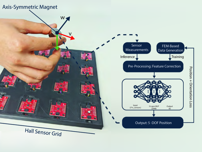
Figure 1: Schematic pipeline overview. We use a Multi-Layer Perceptron (MLP) to output the location and orientation of the magnet directly. During the training phase, the MLP outputs are compared with the FEM ground truth. During the inference, the input to the MLP is the sensor data to track the position and orientation of the magnet.

The core of our contribution is a novel tracking method which utilizes supervised learning. Specially, we use a Multi-Layer Perceptron. Our tracking pipeline has two different instances: during the training phase, the output of the MLP is compared to the labeled data generated by FEM, during device operation (inference), the sensors readings are fed to the MLP to obtain the magnetic marker position and orientation (Figure 1). In this section, we first elaborate on how we create a high-resolution synthetic dataset (Sec. 2.1). Second, we detail our neural network architecture and training (Sec. 2.2). Finally, we describe the hardware setup used for simulation (Sec. 2.3).

2.1 Synthetic Dataset

We focus on permanent magnet localization with axisymmetric symmetry; any shape and size of magnets as long as it possesses rotational symmetry about its magnetization axis. This set includes all cylinders, spheres, and arbitrary cross-section toroids magnetized on its principal axis, enclosing all the most used types of permanent magnets. This symmetry of the magnets allows us to make only one high-resolution 2D FEM simulation for every magnet shape. We revolve this 2D cross-section around its principle axis to obtain the 3D volume then place it anywhere in the space. From a single 2D FEM simulation, we generate synthetic readings for all sensors, with arbitrary location and orientation of the magnet. Such a synthetic dataset results in an improvement of the computational efficiency during training, letting us keep a good balance between granularity in simulation and requiring negligible storage space for the data.

Table 1: Variables used in Algorithm 1.

Variables	Description
$\mathbf{p}^{C}_{i}$	Positional vector. For C and i see below.
$C\in\{D,M\}$	Coordinate system on device ($D$) or magnet ($M$)
$i\in\{s,m\}$	Positional vector of sensor ($S$) or magnet ($m)$
$\mathbf{u,v,w}$	Axis in magnet’s coordinate ($C_{D}$)
$\mathbf{w}$	Magnetic moment direction in $C_{D}$
$\mathbf{B}$	Magnetic flux density

Algorithm 1 Synthethic dataset generation

1:Input $\mathbf{p}^{D}_{s}$

2:$\mathbf{p}_{d}^{D}\leftarrow\mathbf{p}^{D}_{m}-\mathbf{p}^{D}_{s}$ $\triangleright$ Magnet-sensor vector

3:$\mathbf{v}\leftarrow\mathbf{w}\times\mathbf{p}_{d}^{D}$

4:while $\mathbf{v}=\mathbf{0}$ do $\triangleright$ If $\mathbf{w}$ and $\mathbf{p}_{d}^{D}$ are (anti-)parallel

5:     random $\mathbf{q}$

6:     $\mathbf{v}\leftarrow\mathbf{q}\times\mathbf{w}$

7:$\mathbf{u}\leftarrow\mathbf{v}\times\mathbf{w}$

8:$dw\leftarrow\mathbf{p}_{d}^{D}\cdot\frac{\mathbf{w}}{||\mathbf{w}||}$ $\triangleright$ the projection of $\mathbf{p}_{d}^{D}$ on $\mathbf{w}$

9:$du\leftarrow\sqrt{|\mathbf{p}_{d}^{D}|^{2}-dw^{2}}$ $\triangleright$ the projection of $\mathbf{p}_{d}^{D}$ on $\mathbf{u}$

10:$dv\leftarrow 0$

11:$\mathbf{B}^{M}\leftarrow\mathbf{2D-FEM}(du,dw)$

12: $\mathbf{M}\leftarrow\big{[}\begin{smallmatrix}\frac{\mathbf{u}}{||\mathbf{u}||}^{\top}&\frac{\mathbf{v}}{||\mathbf{v}||}^{\top}&\frac{\mathbf{w}}{||\mathbf{w}||}^{\top}\end{smallmatrix}\big{]}^{\top}$ ==== $\triangleright$ Coordinate transformation matrix

13:$\mathbf{B}^{D}\leftarrow\mathbf{B}^{M}\cdot\mathbf{M}$

We used COMSOL Multiphysics to obtain the FEM data. The simulation is centered at the magnet and constrained to only the upper-right half of the cross-section. We obtain the other half of the magnetic field values anti-symmetrically. We use the transformation described in Algorithm 1 to generate the data for training and evaluate the neural network. The algorithm transforms $2$D FEM data into $3$D synthetic readings on each sensor location as follows. First, we input the current position of the magnet and each sensor location, all in a fixed coordinate system ($C_{D}$) centered at the device (L1-L2). Secondly, we build up a coordinate system centered on the magnet’s current position and orientation, $C_{M}$ (L3-L10). Thirdly, the algorithm computes the magnetic flux density $\mathbf{B}^{M}$ at the sensor’s location in $C_{M}$ using the FEM data (L11). Finally, we transform the $\mathbf{B}^{M}$ into the original global coordinates $C_{D}$ to serve as features for training the MLP (L12-L13). All definitions of variables used in Algorithm 1 are described in Table 1.

2.2 Tracking with Neural Networks

2.2.1 Multi-Layer Perceptron

We used a Multi-Layer Perceptron (MLP) as network architecture. The input of the MLP is a $3n$-element vector containing the ($x,y,z$) magnetic flux densities $\mathbf{B}$ of the $n$ sensors. The output is a tuple of $6$ elements composed of the magnet position, $\mathbf{p}=[p_{m}^{x},p_{m}^{y},p_{m}^{z}]$, and its orientation, $\mathbf{o}=[o_{m}^{x},o_{m}^{y},o_{m}^{z}]$. We can then write the MLP as a non-linear mapping from the sensor readings to the tracking variables:

$$\mathcal{F}:\mathbb{R}^{3n}\rightarrow\mathbb{R}^{6};\mathcal{F}(\mathbf{[\mathbf{B}_{1},...,\mathbf{B}_{3n}]})=[\mathbf{p},\mathbf{o}]$$ (1)

Note that even when we have 5-DoF output, three in $\mathbf{p}$ and two in $\mathbf{o}$, we express the orientation vector in cartesian coordinates to avoid the numerical discontinuity when the azimuth angle jumps from $359^{\circ}$ to $0^{\circ}$.

Our MLP architecture is shown in Figure 1. We use a $3$-layer perceptron, with $2048$ units per layer, except for the input and output layers. Rectified linear units are used as activation functions.

2.2.2 Pre-processing

Importantly, we empirically validated that the systems training does not converge if magnetic readings are used directly as inputs. One of the reasons may be that the input values vary by several orders of magnitude when the magnet moves from close to a sensor ( $10^{-2}$ Tesla) to the extension of the working volume ( $10^{-6}$ Tesla). As stated in the dipole model,

$${\mathbf{B}}({{\mathbf{p}}_{m}})=\frac{{{\mu_{0}}}}{{4\pi}}\left[{\frac{{3{\mathbf{r}}({\mathbf{m}}\cdot{\mathbf{r}})}}{{{r^{5}}}}-\frac{{\mathbf{m}}}{{{r^{3}}}}}\right]\,$$ (2)

the magnetic field decays as $1/r^{3}$, where $r$ is the distance between the source and the sensors and $\mathbf{m}$ is the dipole moment. In order to re-scale the input signals, we take the cubic root of the input data, $f(B)=\sqrt[3]{B}$ (see Figure 1). We found that training with cubic root re-scaling convergences in $\sim 40$ epochs.

2.2.3 Training Loss

We train the neural networks with randomly sampled data in a cubic volume, $0.2\times 0.2\times 0.15$ m³, with the sensor array covering the bottom face. The magnets’ orientation is sampled as points on a unit sphere, then paired with the locations as labels for training. Then, the labeled data for training is obtained as in Algorithm 1. As loss function we used the weighted sum of positional and orientation differences averaged over all $n$ points in a training batch:

$$\mathcal{L}=\frac{1}{n}\sum_{i=1}^{n}\big{(}\|\mathbf{p}_{true}-\mathbf{p}_{pred}\|^{2}+\eta\|\frac{\mathbf{o}_{true}}{\|\mathbf{o}_{true}\|}-\frac{\mathbf{o}_{pred}}{\|\mathbf{o}_{pred}\|}\|^{2}\big{)}$$ (3)

where we aim to minimise both the positional and oriental disparity between the prediction and ground truth. We add the weight $\eta$ to compensate for different orientation and positional error term scales. From parameter tuning, we find $\eta=10^{-5}$ and use it as a default in all experiments.

We implement the MLP in python with PyTorch. The optimizer Adam [28] is adopted with an initial learning rate $\gamma=10^{-4}$. We train for 40 epochs, and the learning rate decays by $0.98$ after each epoch in training. We generate $10^{6}$ random points per epoch to train the model with a batch size of $256$. Using Algorithm 1 we generate the training data independently and identically distributed. Data generation and training of the MLP takes $\sim 1$ hour.

2.3 Hardware Implementation

The core of our hardware comprises $16$ triaxial magnetometers (MLX90393, Malexis). They have a linear range up to $0.05$ Tesla, which is compatible with the magnetic fields we expected from our testing magnets at close range. While the sensors allow for a data output rate of $716.9$ Hz, our default configuration is set to $35.4$ Hz. We also set the sensors to the $0-10^{-1}$ Tesla range, covering most of the cases when sensing locations are $\geq 2$ cm away from the magnets. In addition, we use the ellipsoid-fitting method in [29] to calibrate our system. The 16 sensors are placed in a $4\times 4$ grid with an interval of $52$ mm between the centers of neighboring sensors, as shown if Figure 2(a).

To keep instrumentation low and enable portable applications, e.g. prosthetics, we implemented the tracking inference in a AI-oriented single board computer (Jetson Nano, NVIDIA). This device only weights 138 grams and also allows for reading the sensors directly using the I2C communication protocol. The lower bound of time of reading $16$ sensors sequentially is in the order of $24$ milliseconds.

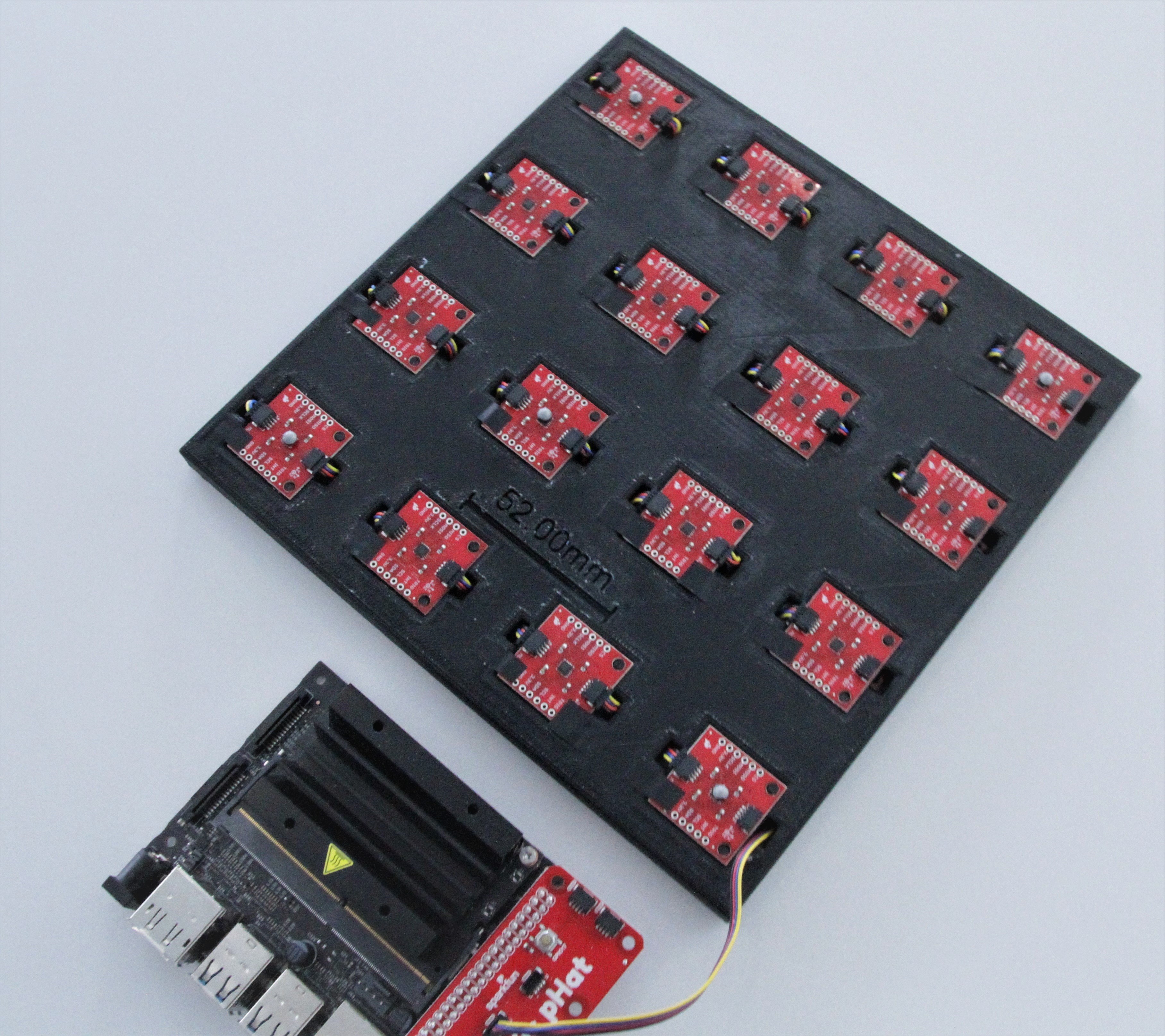
Figure 2: Hall sensor array in a 4x4 grid. The center-to-center distance is 52mm. The array is connected to a Jetson Nano for the complete inference pipeline. The inset shows a rigid-tree to collect Optitrack groundtruth.

3 Comparison between our data-driven and an optimization-based tracking

In this section, we contrast the performances of our neural network tracking method with an iterative gradient-descent based technique. Performing this comparison with simulated sensor readings allows us to control experimental conditions such as the initialization of the iterative optimization-based algorithm. The data is also noise-free, thus comparing the ideal performance of the two methods.

The optimization uses PyTorch with the magnet position and orientation set as variables with automatic differentiation [30] enabled. For the optimizer, we select L-BFGS [31], a quasi-Newton method, with line search to establish the optimal step size. The internal physical model to evaluate magnetic fields is the magnetic dipole model, implemented as in the loss function as proposed in [13].

For a fair comparison, we distinguish two cases: i) we train the MLP network using the FEM data, and ii) using the magnetic dipole model directly, which is equivalent to the optimization method model. Furthermore, we show the results obtained via the optimization-based method for different initialization errors. Finally, we compare the running time of the two approaches for tracking synthetic data.

3.1 Influence of initialization on the optimization methods

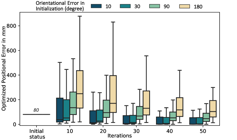
(a)

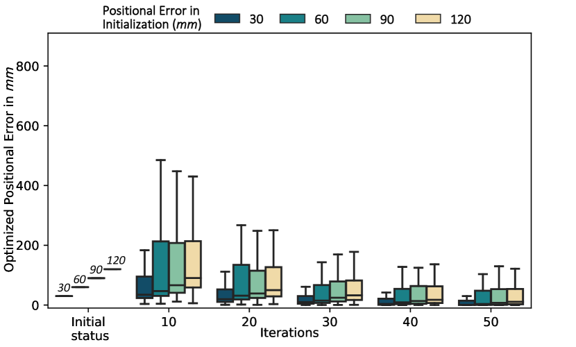
(b)

Figure 3: Positional errors of the iterative method in simulation for different number of iterations. (a) We vary to initial orientation mismatch keeping a fixed distance of $80$ mm to the truth. (b) We vary the positional error initialization keeping a fixed orientation difference of $45^{\circ}$.

For this evaluation, we randomly sample the magnet’s positions and orientations as in Section 2.2.3, and we compute corresponding magnetic flux densities with the magnetic dipole model at the locations of sensors (Eq. 2). In this way, the characteristics of the synthetic signals agree with the internal physical model in the optimization method. To have the initial guess in optimization, we disturb this target position and orientation. We configure the iterative algorithm so the optimization stops when reaching the maximal number of iterations we allowed.

In Figure 3 we present the results for the optimization method, reporting the tracking errors as a function of the of the maximal number of iteration for different values of positional miss-match (Figure 3.a) and orientation miss-match (Figure 3.b). Each box-plot is based in $400$ randomly target positions and orientations.

For detailed analysis, we report the statistics of tracking results after $50$ iterations in Table 2 (corresponding with the right most set of results in Figure 3). At the bottom of table we include the position and orientation errors for the same synthetic readings using our MLP method. Note that MLPs do not require an initial estimation of the position and orientation of the magnet. They are independent of the initialization, as it is not part of their feature vector.

Our MLP is outperformed only in the cases with most iterations (50), and with the best initialization: $80$ mm of initial positional error and $10^{\circ}$ of initial orientation error, and $30$ mm of initial positional error and $45^{\circ}$ of initial orientation error. However, the computational time of this optimization-based method is about 50x longer than the time consumed by predicting via the MLP (see Sec. 3.2).

When we reduce the number of iterations, the error increases considerably. With only ten iterations, the median positional error exceeds $200$ mm in some cases, especially when the seed orientation is far from the target. However, we find that even in cases where the initial orientation is close to the target (the error is $45^{\circ}$), the positional errors obtained are as large as the miss-match in initialization.

Table 2: Accuracy results for the iterative method after 50 Iterations. For comparison, we include results obtained via MLP tracking on the same evaluation data.

Initial $e_{p}$ in mm	Initial $e_{\theta}$ in degrees	$\ \mathtt{median}$ $e_{p}$ in mm	$\mathtt{median}$ $e_{\theta}$ in degrees	$\mathtt{3^{rd}quartile}$ $e_{p}$ in mm	$\mathtt{3^{rd}quartile}$ $e_{\theta}$ in degrees
Iter. Optimization
80	10	0.92	1.63	32.96	9.98
80	30	4.17	8.54	47.17	29.99
80	90	40.83	87.16	83.80	90.00
80	180	90.88	179.90	158.11	179.99
30	45	0.42	0.74	12.86	36.12
60	45	3.19	6.89	33.47	44.84
90	45	6.62	15.17	41.29	44.91
120	45	10.47	28.94	59.43	45.01
MLP (ours)
–	–	1.34	3.45	1.91	5.16

3.2 Running Time

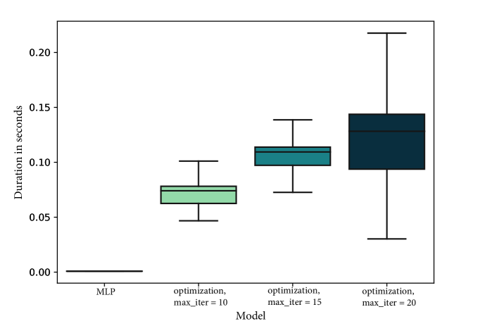
Figure 4: Inference time comparison between MLP and L-BFGS implementations for a different number of iterations. Iterative methods are strongly dependent on initialization and it takes between 20 and 50 iterations (i.e. $>$ 10 ms) to achieve results similar to those given by a single MLP inference (0.8 ms).

Our MLP implementation produces readings after a single inference step involving feature engineering, additions, and multiplications in hidden layers. In contrast, optimization-based methods require computations of second-order gradients concerning the estimated locations of every iteration until it converges. We compare here the differences in speed in our two tested methods.

In Figure 4 we compare the end-to-end time of our data-driven method (MLP) vs different maxmimum number of iterations steps of the optimization-based algorithm we implemented. One 5 DoF tracking inference in MLP takes $0.8$ ms, including the feature engineering process. In contrast, the L-BFGS optimizer takes around $1$ ms for each iteration. As shown in Figure 3, we need $10$s of iterations to achieve satisfying results depending on the initialization. This results in $10$s of milliseconds. We note that for this particular speed comparison, we run both methods on the same laptop with an Intel i7-7500U CPU.

3.3 Neural Networks trained with FEM vs Dipole Model

In previous works authors train MLPs on data generated with the magnetic dipole model. In this work, we propose a step forward by modeling beyond the dipole approximation and take full advantage of the powerful representation of Neural Networks for non-linear systems. We propose six different shapes of magnets for our evaluation, identical to those we adopt in hands-on experiments in Section 4. The selection goes from very tall bars to very flat disks, all magnetized in the principal axis, plus a sphere, given that the dipole model is the exact solution in this last case. We use $1000$ points per magnet to evaluate the position error, and the target positions and orientations are identical for all $6$ magnets.

In Figure 5 we compare the performance of our MLP method when trained with two different synthetic datasets: one obtained FEM simulations as explain in Section 2.1, and the other using the magnetic dipole approximation (Eq. 2). The shapes of magnets are ordered from tall bar-shape to thin disc-shaped, getting closer to a spherical shape and then deviating from it. We used a Shapiro-Wilk test to validate the normal distribution of our data and then applied a Student’s T-Test to test for significant differences between dipole- and FEM-data trained MLPs.

We found significant differences in all cases of cylindrical magnets and no significant difference for the spherical magnet. The p-values of the Student’s T-Tests are $<.005$ with the exception of the spherical case ($p=0.95$). As expected, we observed greater differences in the results as the shape of the magnet distances itself from the sphere.

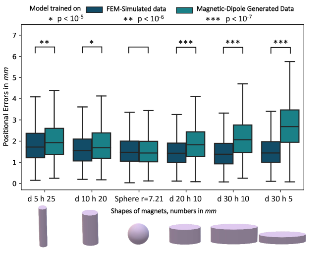
Figure 5: Comparison of positional errors on MLP neural networks when trained with FEM- or dipole model-generated datasets.

4 Experimental Evaluation

In this evaluation, we compare the results of our MLP tracking method to experimental ground truth data collected with Optitrack. Apart from evaluating accuracy in position and orientation, we present the speed performance in this portable computer considering both the data-collection process and the inference process running simultaneously on the same device.

4.1 Magnetic plus Optical Tracking Setup

The magnetic tracking hardware consists of 16 magnetic sensors distributed in a 4 x 4 array and a Jetson Nano portable computer to read the sensors and perform MLP inferences. For details see Section 2.3. The permanent magnet is attached to a tree-shaped 3D-printed holder, which holds five IR reflective markers on its branches to collect the ground-truth data (as in the inset of Figure 2). We use ten OptiTrack cameras to track this rigid body, and the cylindrical magnets used here are the same as the simulated in Section 3.3.

During the experiment, the magnet is moved and tilted freely in the space over the sensor array while ensuring that the cameras capture most of the optical markers. The speed of moving is comparable to playing games with joysticks. For those cases where we compare different numbers of sensors, we log the readings from the sensors array which are then fed offline into MLPs with varying input dimensions. We correct the time-sync mismatch between two tracking systems by adjusting a time-offset variable in the magnetic signals and by searching for the lowest tracking error during a calibration step. In addition, we use PCHIP interpolation [32] to adjust difference in the sampling frequency.

4.2 Results

In Figure 6 we show a single trajectory tracked via our MLP method as well as optitrack clipped within the same time range. For this particular trajectory we use the magnet with diameter $10$mm, height $20$ mm ($d\ 10\ h\ 20$). The deviation between the two trajectories is within the $4$ mm limit more than half of the time, with the largest deviation happening in fast turns and never exceeding $10$ mm. We note that the discontinuities in the OptiTrack trajectories come from partial occlusion of the IR markers. In figure 7, we show the statistics of tracking results obtained from five different cylindrical magnets. As expected, the higher the number of sensors deployed, the lower the tracking errors for all the magnets tested. When we use the full set of $16$ sensors, the average tracking errors in position and orientation are generally smaller than $4$ mm and $8^{\circ}$, except for the pole-shape magnet ($d\ 5\ h\ 25$).

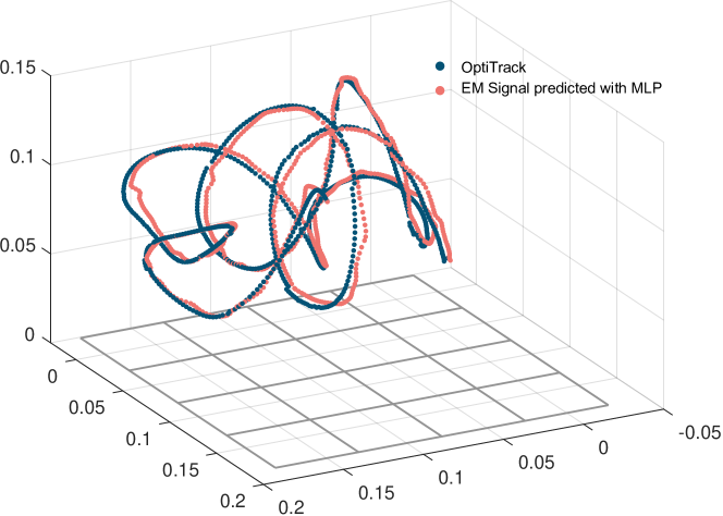
Figure 6: Comparison of trajectories obtained by OptiTrack and MLP. The difference is generally smaller than 4mm

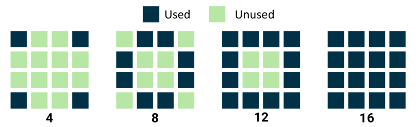
(a)

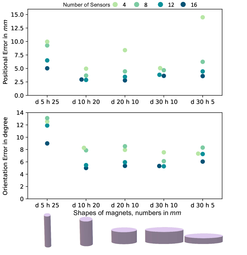
(b)

Figure 7: Experimental positional and orientation errors obtained with MLP tracking, for different numbers of input sensor and magnet shapes.

Finally, we conduct experiments to test the interactive frequency of our method when the inference is done either on the CPU or the GPU of Jetson Nano. Note that process of reading sensors is always running on the CPU via the I2C protocol, giving an average time of $1.75$ ms per sensor. For the inference process, the duration of inference running on the CPU is around $28$ ms and stays relatively steady as the dimension of input features increases. When the inference runs on GPU, the duration for the prediction process increases from $10$ ms when using 4 sensors to $15$ ms when using the complete set of 16 sensors.

5 Discussion

In Section 3.1 we recovered a known shortcoming in iterative methods: tracking accuracy is highly dependent on the seed, particularly in the initial orientation of the magnet. The optimization tends to fall into a local minimum when the first orientation estimate is far from the actual value. In contrast, Figure 3 shows that with a relatively good first orientation (miss-match less than $45^{\circ}$), the convergence is less sensitive to other perturbations. In results after 50 iteration steps (Table 2), the $3^{rd}$ quartile errors are as large as the initialization errors, showcasing that the optimization method might fail to reach the global minimum after $50$ epochs.

On the other hand, tracking via neural networks is initialization-independent. In Table 2 we see that MLP can outperform the optimization-based method, except for the cases with the most reliable initial estimation and the maximum number of iterations. Moreover, the maximal positional and orientation errors are all bounded by acceptable limits when tracking via MLP, testifying to its stability.

When deploying our method in an experimental prototype, tracking errors are only slightly increased due to noise in the actual sensors: see Figure 5 (training via FEM) and Figure 7 (for $N_{sensors}=16$). We plot in Figure 8 the results of positional error obtained in Section 4 as a function of the distance to the center of array, showing that the method is robust even at large distances. It is remarkable how we could directly use the models trained with simulations in the experimental tests without fitting any hyperparameters. We leave for future work the possibility of including background and sensor noise during the training of the neural networks, similar to what has been shown in other magnetic tracking systems [33, 34]. This will reduce the sim-to-real mismatch, improving accuracy of the MLP method.

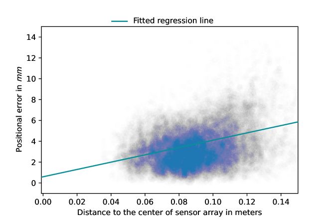
Figure 8: Positional tracking errors versus distance between the magnet position and the center of the array.

In Section 3.3, we tested the effect of using training datasets generated via FEM or the magnetic dipole model. As expected, the dipole model has closer performances to FEM-trained models when the magnet is in shape closer/equal to a sphere, testified by more significant p-values of Student’s T-tests. For magnets of cylindrical shapes, FEM-Simulated trained models improve the tracking by $0.2$ mm to $1.2$ mm. We observe, however, that the tracking performance of MLP also degrades as the magnets shapes differ more from a sphere (see Figure 7, may be due to demagnetizing factors not included in this work.

We observe that the one-shot inference total time in MLP is comparable to each (of the many) optimization steps of the iterative methods (Section 3.2). As remarkable as its speed, the MLP can be called on demand, sporadically, without the need to keep the target tracked and locked in order to ensure a correct convergence within a few iteration steps. We also show that it is possible to implement a MLP tracking algorithm on a portable, energy-constrained device. We notice that the inference time via GPU takes about the same time than reading $8$ sensors via the I2C protocol via the CPU. Therefore, the sensor reading process throttles the refresh rate of the current prototype. Protocols such as SPI can improve this issue.

A shortcoming of data-driven methods is that the neural network needs to be retrained every new condition, e.g., different amount of sensors and their placements or when the magnet shape is changed. Although our training take only $\sim 1$ hour including data generation, it prevents some applications such as the online optimization of sensor location.

6 Conclusion

In this paper, we show the accuracy and efficiency of using neural networks to directly predict the location and orientation of magnets. We combine 2D FEM-simulated data with a coordinate transformation algorithm to generate on-demand synthetic training for any type of axis-symmetric magnet. The tracking performed by neural networks is stable and does not suffer from convergence failure in optimization-based tracking. When conducting hands-on experiments, the average positional error is generally smaller than $4$ mm within the entire working volume. While now we run at $35$ Hz, this frequency could be doubled by moving to another sensor’s reading protocol. The experiments show that we can now move the tracking algorithms to run on an energy-restricted device and make interactive magnetic applications portable. Promising future research directions include using neural networks to track multiple magnets, using the prediction of neural networks to initialize optimization-based methods, and investigating recurrent neural networks to improve temporal consistency.

References

- [1] X. Han, H. Seki, Y. Kamiya, and M. Hikizu, “Wearable handwriting input device using magnetic field,” in SICE Annual Conference 2007. IEEE, 2007, pp. 365–368.
- [2] Y. Ma, Z.-H. Mao, W. Jia, C. Li, J. Yang, and M. Sun, “Magnetic hand tracking for human-computer interface,” IEEE Transactions on Magnetics, vol. 47, no. 5, pp. 970–973, 2011.
- [3] K.-Y. Chen, S. N. Patel, and S. Keller, “Finexus: Tracking precise motions of multiple fingertips using magnetic sensing,” in Proceedings of the 2016 CHI Conference on Human Factors in Computing Systems, 2016, pp. 1504–1514.
- [4] J. McIntosh, P. Strohmeier, J. Knibbe, S. Boring, and K. Hornbæk, “Magnetips: Combining fingertip tracking and haptic feedback for around-device interaction,” in Proceedings of the 2019 CHI Conference on Human Factors in Computing Systems, 2019, pp. 1–12.
- [5] T. Langerak, J. J. Zárate, D. Lindlbauer, C. Holz, and O. Hilliges, “Omni: Volumetric sensing and actuation of passive magnetic tools for dynamic haptic feedback,” in Proceedings of the 33rd Annual ACM Symposium on User Interface Software and Technology, ser. UIST ’20. New York, NY, USA: Association for Computing Machinery, 2020, p. 594–606. [Online]. Available: https://doi.org/10.1145/3379337.3415589
- [6] S. Krueger, H. Timinger, R. Grewer, and J. Borgert, “Modality-integrated magnetic catheter tracking for x-ray vascular interventions,” Physics in Medicine & Biology, vol. 50, no. 4, p. 581, 2005.
- [7] M. Salerno, R. Rizzo, E. Sinibaldi, and A. Menciassi, “Force calculation for localized magnetic driven capsule endoscopes,” in 2013 IEEE International Conference on Robotics and Automation. IEEE, 2013, pp. 5354–5359.
- [8] Z. Sun, L. Maréchal, and S. Foong, “Passive magnetic-based localization for precise untethered medical instrument tracking,” Computer methods and programs in biomedicine, vol. 156, pp. 151–161, 2018.
- [9] A. Z. Taddese, P. R. Slawinski, M. Pirotta, E. De Momi, K. L. Obstein, and P. Valdastri, “Enhanced real-time pose estimation for closed-loop robotic manipulation of magnetically actuated capsule endoscopes,” The International journal of robotics research, vol. 37, no. 8, pp. 890–911, 2018.
- [10] X. Luo, C. Shi, H.-Q. Zeng, H. C. Ewurum, Y. Wan, Y. Guo, S. Pagnha, X.-B. Zhang, Y.-P. Du, and X. He, “Evolutionarily optimized electromagnetic sensor measurements for robust surgical navigation,” IEEE Sensors Journal, vol. 19, no. 22, pp. 10 859–10 868, 2019.
- [11] F. S. Parizi, E. Whitmire, and S. Patel, “Auraring: Precise electromagnetic finger tracking,” Proceedings of the ACM on Interactive, Mobile, Wearable and Ubiquitous Technologies, vol. 3, no. 4, pp. 1–28, 2019.
- [12] D. Son, S. Yim, and M. Sitti, “A 5-d localization method for a magnetically manipulated untethered robot using a 2-d array of hall-effect sensors,” IEEE/ASME Transactions on Mechatronics, vol. 21, no. 2, pp. 708–716, 2015.
- [13] C. R. Taylor, H. G. Abramson, and H. M. Herr, “Low-latency tracking of multiple permanent magnets,” IEEE Sensors Journal, vol. 19, no. 23, pp. 11 458–11 468, 2019.
- [14] S. Hashi, M. Toyoda, S. Yabukami, K. Ishiyama, Y. Okazaki, and K. I. Arai, “Wireless magnetic motion capture system for multi-marker detection,” IEEE transactions on magnetics, vol. 42, no. 10, pp. 3279–3281, 2006.
- [15] C. Hu, M. Q. Meng, and M. Mandal, “Efficient magnetic localization and orientation technique for capsule endoscopy,” in 2005 IEEE/RSJ International Conference on Intelligent Robots and Systems, 2005, pp. 628–633.
- [16] T. D. Than, G. Alici, H. Zhou, and W. Li, “A review of localization systems for robotic endoscopic capsules,” IEEE Transactions on Biomedical Engineering, vol. 59, no. 9, pp. 2387–2399, 2012.
- [17] M. Yousefi, H. Nejat Pishkenari, and A. Alasty, “A fast and robust magnetic localization technique based on elimination of the orientation variables from the optimization,” IEEE Sensors Journal, vol. 21, no. 19, pp. 21 885–21 892, 2021.
- [18] H.-C. Kuo, R.-H. Liang, L.-F. Lin, and B.-Y. Chen, “Gaussmarbles: spherical magnetic tangibles for interacting with portable physical constraints,” in Proceedings of the 2016 CHI Conference on Human Factors in Computing Systems, 2016, pp. 4228–4232.
- [19] R.-H. Liang, K.-Y. Cheng, C.-H. Su, C.-T. Weng, B.-Y. Chen, and D.-N. Yang, “Gausssense: attachable stylus sensing using magnetic sensor grid,” in Proceedings of the 25th annual ACM symposium on User interface software and technology, 2012, pp. 319–326.
- [20] K.-Y. Chen, K. Lyons, S. White, and S. Patel, “utrack: 3d input using two magnetic sensors,” in Proceedings of the 26th annual ACM symposium on User interface software and technology, 2013, pp. 237–244.
- [21] A. J. Petruska and J. J. Abbott, “Optimal permanent-magnet geometries for dipole field approximation,” IEEE Transactions on Magnetics, vol. 49, no. 2, pp. 811–819, 2013.
- [22] N. Sebkhi, N. Sahadat, S. Hersek, A. Bhavsar, S. Siahpoushan, M. Ghoovanloo, and O. T. Inan, “A deep neural network-based permanent magnet localization for tongue tracking,” IEEE Sensors Journal, vol. 19, no. 20, pp. 9324–9331, 2019.
- [23] A.-i. Sasaki and E. Ohta, “Magnetic-field-based position sensing using machine learning,” IEEE Sensors Journal, vol. 20, no. 13, pp. 7292–7302, 2020.
- [24] A. Mendizabal, P. Márquez-Neila, and S. Cotin, “Simulation of hyperelastic materials in real-time using deep learning,” Medical image analysis, vol. 59, p. 101569, 2020.
- [25] E. Haghighat, M. Raissi, A. Moure, H. Gomez, and R. Juanes, “A deep learning framework for solution and discovery in solid mechanics,” arXiv preprint arXiv:2003.02751, 2020.
- [26] G. Psuj, “Multi-sensor data integration using deep learning for characterization of defects in steel elements,” Sensors, vol. 18, no. 1, p. 292, 2018.
- [27] I. Malkiel, M. Mrejen, A. Nagler, U. Arieli, L. Wolf, and H. Suchowski, “Plasmonic nanostructure design and characterization via deep learning,” Light: Science & Applications, vol. 7, no. 1, pp. 1–8, 2018.
- [28] D. P. Kingma and J. Ba, “Adam: A method for stochastic optimization,” arXiv preprint arXiv:1412.6980, 2014.
- [29] T. Pylvänäinen, “Automatic and adaptive calibration of 3d field sensors,” Applied Mathematical Modelling, vol. 32, no. 4, pp. 575–587, 2008.
- [30] A. G. Baydin, B. A. Pearlmutter, A. A. Radul, and J. M. Siskind, “Automatic differentiation in machine learning: a survey,” Journal of machine learning research, vol. 18, 2018.
- [31] D. C. Liu and J. Nocedal, “On the limited memory bfgs method for large scale optimization,” Mathematical programming, vol. 45, no. 1, pp. 503–528, 1989.
- [32] K. Brodlie and S. Butt, “Preserving convexity using piecewise cubic interpolation,” Computers & Graphics, vol. 15, no. 1, pp. 15–23, 1991.
- [33] G. Shao, Y. Tang, L. Tang, Q. Dai, and Y.-X. Guo, “A novel passive magnetic localization wearable system for wireless capsule endoscopy,” IEEE Sensors Journal, vol. 19, no. 9, pp. 3462–3472, 2019.
- [34] Q. Li, Z. Shi, Z. Li, H. Fan, G. Zhang, and T. Li, “Magnetic object positioning based on second-order magnetic gradient tensor system,” IEEE Sensors Journal, vol. 21, no. 16, pp. 18 237–18 248, 2021.