Closed string mirrors of symplectic cluster manifolds

Abstract.

We compute the relative symplectic cohomology sheaf in degree $0$ on the bases of nodal Lagrangian torus fibrations on four dimensional symplectic cluster manifolds. We show that it is the pushforward of the structure sheaf of a certain rigid analytic manifold under a non-archimedean torus fibration. The rigid analytic manifold is constructed in a canonical way from the relative SH sheaf and is referred as the closed string mirror. The construction relies on computing relative SH for local models by applying general axiomatic properties rather than ad hoc analysis of holomorphic curves. These axiomatic properties include previously established ones such as the Mayer-Vietoris property and locality for complete embeddings; and new ones such as the Hartogs property and the holomorphic volume form preservation property of wall crossing in relative $SH$.

1. Introduction

Let $M$ be a geometrically bounded symplectic $4$-manifold equipped with a Lagrangian torus fibration with focus-focus singularities $\pi:M\to B$. Fix a commutative ring $\mathbb{F}$ and let $\Lambda_{\geq 0}:=\mathbb{F}[[T^{\mathbb{R}}]]$ be the Novikov ring over it. To any compact $P\subset B$ is associated a $\mathbb{Z}$-graded $\Lambda_{\geq 0}$-algebra $SH^{*}_{M}(\pi^{-1}(P)),$ the relative symplectic cohomology of $\pi^{-1}(P)$. Results of [28] imply that if we consider the $G$-topology of compact sets on $B_{\mathcal{R}}$, the assignment $P\mapsto SH^{0}_{M}(\pi^{-1}(P))$ along with the natural restriction maps form a sheaf.

In this paper, we assume the induced integral affine structure with singularities on $B$ is isomorphic to $B_{\mathcal{R}}$ for some eigenray diagram $\mathcal{R}$. We will always consider a weaker $G$-topology on $B_{\mathcal{R}}$, the $G$-topology of admissible polygons. Admissible opens in this topology are (roughly speaking) finite unions of convex, possibly degenerate, rational polygons such that if they contain a node, then they contain only one node which is an interior point in the standard topology of $B_{\mathcal{R}}$. Admissible coverings are finite covers of admissible polygons by admissible polygons. See Section 2 for definitions and more details.

The aim of this paper is to fully describe the sheaf of algebras over $\Lambda:=\mathbb{F}((T^{\mathbb{R}}))$ defined by:

$$\mathcal{F}(P):=SH^{0}_{M}(\pi^{-1}(P);\Lambda)=SH^{0}_{M}(\pi^{-1}(P))\otimes_{\Lambda_{\geq 0}}\Lambda$$

and use it to reconstruct in a canonical way a non-archimedean analytic mirror of $M$ and some of its related structures.

In our discussions involving non-archimedean geometry, we will assume for simplicity that $\mathbb{F}$ is a characteristic $0$ algebraically closed field, which implies that $\Lambda$ is also an algebraically closed field [7, Appendix 1]. Let $\mathcal{Y}$ be a rigid analytic space over $\Lambda$ in the sense of Tate and $B$ a nodal integral affine manifold. We call a map $p:\mathcal{Y}\to B$ continuous if the preimage of each admissible polygon is an admissible open of $\mathcal{Y}$ and the preimages of admissible coverings are admissible coverings in $\mathcal{Y}$. We call such a continuous map Stein if around every $b\in B$ there is an admissible convex polygon $P_{b}$ which contains $b$ in its interior such that for any admissible convex $Q\subset P_{b}$, the rigid analytic space $p^{-1}(Q)$ is isomorphic to an affinoid domain.

Theorem 1.1.

Let $\pi_{\mathcal{R}}:M_{\mathcal{R}}\to B_{\mathcal{R}}$ be a Lagrangian fibration associated to an eigenray diagram $\mathcal{R}$. There exists a canonical rigid analytic space $\mathcal{Y}_{\mathcal{R}}$ over $\Lambda$ with a Stein continuous map $p_{\mathcal{R}}:\mathcal{Y}_{\mathcal{R}}\to B_{\mathcal{R}}$ such that the push-forward under $p_{\mathcal{R}}$ of the structure sheaf of $\mathcal{Y}$ is isomorphic to the sheaf

$$\mathcal{F}_{\mathcal{R}}(P):=SH^{0}_{M_{\mathcal{R}}}(\pi_{\mathcal{R}}^{-1}(P);\Lambda).$$

Moreover,

1. $p_{\mathcal{R}}:\mathcal{Y}_{\mathcal{R}}\to B_{\mathcal{R}}$ is an affinoid torus fibration in the complement of the set of nodal points $N_{\mathcal{R}}\subset B_{\mathcal{R}}$.

2. The space $\mathcal{Y}_{\mathcal{R}}$ is smooth if and only if the nodes of $\mathcal{R}$ all have multiplicity $1$, which is equivalent to $\pi_{\mathcal{R}}$ having at most one critical point in each fiber.

3. There is a canonical volume form $\Omega_{\mathcal{R}}$ on the smooth locus of $\mathcal{Y}_{\mathcal{R}}$.

4. Let $\mathcal{R}_{1}$ and $\mathcal{R}_{2}$ be eigenray diagrams related by a branch move. Then, we have an analytic isomorphism $\mathcal{Y}_{\mathcal{R}_{1}}\simeq\mathcal{Y}_{\mathcal{R}_{2}}$ intertwining the torus fibrations and the volume forms.

5. Let $\mathcal{R}_{1}$ and $\mathcal{R}_{2}$ be eigenray diagrams related by a nodal slide that preserve all the multiplicities. Then, we have an analytic isomorphism $\mathcal{Y}_{\mathcal{R}_{1}}\simeq\mathcal{Y}_{\mathcal{R}_{2}}$ between the associated mirrors. The isomorphism intertwines the volume forms, but not the torus fibrations.

6. The symplectic invariant $SH_{M_{\mathcal{R}}}^{0}(M_{\mathcal{R}},\Lambda)$ is isomorphic as a $\Lambda$-algebra to the algebra of entire functions on $\mathcal{Y}_{\mathcal{R}}$.

Remark 1.2.

In Theorem 1.1 item (5) it is important that we consider only paths where the multiplicities of nodes are not changed. See Remark 1.9 for what happens when multiplicities are modified by nodal sliding.

Remark 1.3.

We do not claim that the preimage under $p_{\mathcal{R}}$ of every admissible convex polygon $P$ is an affinoid domain, only when it is sufficiently small (see the definition of a small admissible polygon in Section 2.2 and Proposition 10.2). Tony Yue Yu informed us that a straightforward induction based on [30, Proposition 6.5] shows that when $P$ does not contain a node, then indeed the preimage is always an affinoid domain.

Remark 1.4.

We could extend the isomorphism of sheaves result to a finer $G$-topology on $B_{\mathcal{R}}$ by defining our admissible opens to be arbitrary unions of admissible convex opens with a certain locally finiteness assumption as in the standard extension of the weak $G$-topology on an affinoid domain to its strong $G$-topology [3, Definition 4]. The property (6) would then be the specialization of the isomorphism of sheaves to the admissible open that is the entire set.

1.1. The construction

We will abbreviate $MaxSpec$ by $M$ in this paper and for $A$ an affinoid algebra, we will denote by $M(A)$ the corresponding affinoid domain.

The underlying set of the rigid analytic variety $\mathcal{Y}_{\mathcal{R}}$ of Theorem 1.1 has the following simple description. For each admissible convex polygon denote by $M(P):=M(\mathcal{F}_{\mathcal{R}}(P))$ the set of maximal ideals of $\mathcal{F}_{\mathcal{R}}(P)$. Given a cover $\mathcal{U}$ of $B$ by admissible convex polygons let $\mathcal{Y}_{\mathcal{U}}:=\coprod_{P\in\mathcal{U}}\mathcal{M}_{P}/\sim$ where the gluing is by relation on generated by identifying $x\in\mathcal{M}(P)$ with $y\in\mathcal{M}(Q)$ whenever there is a $z\in\mathcal{M}(P\cap Q)$ mapping to $x,y$ respectively under the restriction maps $\mathcal{F}(P)\to\mathcal{F}(P\cap Q)$ and $\mathcal{F}(Q)\to\mathcal{F}(P\cap Q)$. If $\mathcal{U}^{\prime}$ is a refinement of $\mathcal{U}$ there is a natural map $\mathcal{Y}_{\mathcal{U}^{\prime}}\to\mathcal{Y}_{\mathcal{U}}$. We this define $\mathcal{Y}:=\varprojlim_{\mathcal{U}}\mathcal{Y}_{\mathcal{U}}$.

We refer to this as the closed string mirror. Note that it is not a priori clear that this construction gives rise to a rigid analytic variety. For this we need to know first of all that the gluing relation is actually an equivalence relation. In addition, we need to know that for $Q\subset P$ small enough $\mathcal{F}(P)$ is affinoid and the restriction map $\mathcal{F}(P)\to\mathcal{F}(Q)$ induces an inclusion of an affinoid subdomain.

The following theorem gives the necessary properties. In the statement we refer to the notion of a small admissible polygon whose definition appears in Section 2.2.

Theorem 1.5.

For $\mathcal{R}$ an eigenray diagram, the sheaf $\mathcal{F}_{\mathcal{R}}$ satisfies the following properties

• (Affinoidness) If $P$ is a small admissible polygon, $\mathcal{F}_{\mathcal{R}}(P)$ is an affinoid algebra.

• (Subdomain) If $Q\subset P$ are small admissible polygons, then the morphism of affinoid domains induced from the restriction map $\mathcal{F}_{\mathcal{R}}(P)\to\mathcal{F}_{\mathcal{R}}(Q)$:

  $$M(\mathcal{F}_{\mathcal{R}}(P))\to M(\mathcal{F}_{\mathcal{R}}(Q))$$

  has image an affinoid subdomain and it is an isomorphism of affinoid domains onto its image.

• (Strong cocycle condition) For small admissible polygons $Q,Q^{\prime}\subset P$, we have

  $$im(M(\mathcal{F}_{\mathcal{R}}(Q))\cap im(M(\mathcal{F}_{\mathcal{R}}(Q^{\prime})))=im(M(\mathcal{F}_{\mathcal{R}}(Q\cap Q^{\prime}))$$

  inside $M(\mathcal{F}_{\mathcal{R}}(P)).$

• (Independence) Let $Q_{1},\ldots,Q_{N}\subset P$ be small admissible polygons such that $P=\bigcup Q_{i}$. Then

  $$\bigcup im(M(\mathcal{F}_{\mathcal{R}}(Q_{i})))=M(\mathcal{F}_{\mathcal{R}}(P)).$$

• (Separation) Let $Q\subset P$ be an inclusion of small admissible polygons. For any $p\in M(\mathcal{F}_{\mathcal{R}}(P))\setminus im(M(\mathcal{F}_{\mathcal{R}}(Q))$ there is a small admissible polygon $Q^{\prime}\subset P$ which is disjoint of $Q$ such that $p\in im(M(\mathcal{F}_{\mathcal{R}}(Q^{\prime})))$.

The above theorem allows us to endow the closed string mirror with a $G$-topology and a structure sheaf turning it into a rigid analytic variety. In addition we show that any rigid analytic variety $X$ constructed from a sheaf $\mathcal{F}$ on $B_{\mathcal{R}}$ satisfying the above properties is endowed with a Stein continuous map $p:X\to B_{\mathcal{R}}$ so that there is a canonical isomorphism of sheaves of $\Lambda$-algebra $\mathcal{F}\simeq p_{*}\mathcal{O}_{X}$.

Remark 1.6.

The proof of Theorem 1.5 relies on local computations and results of [9] concerning locality of relative SH for complete embeddings. More details are given in the next subsection. We pose the following

Question.

Is it possible to prove the properties in Theorem 1.5 as a priori properties of the sheaf $\mathcal{F}$ without first computing?

We expect the answer is positive for singular Lagrangian torus fibrations satisfying some natural hypotheses. See Section 11 for one class of examples. This is pursued in other work.

Remark 1.7.

There is alternative approach to constructing the closed string mirror. Namely, we could define the underlying set of the mirror as

$$\mathcal{Y}=\coprod_{b\in B_{\mathcal{R}}}M(\mathcal{F}_{\mathcal{R}}(\{b\})).$$

We expect this construction is correct for more general Lagrangian torus fibrations provided neighborhoods of singular fibers are modeled on Liouville domains equipped with a radiant Lagrangian torus fibration whose Liouville field lifts the Euler vector field in the base. The construction would have a number of conceptual advantages. Among other things, there is no need to establish the cocycle condition, and the function $p_{\mathcal{R}}:\mathcal{Y}\to B_{\mathcal{R}}$ is obvious from the construction. However, in order to endow $\mathcal{Y}$ with the structure of a rigid analytic variety we still need to show that for sufficiently small polygons $P$ the natural restriction maps $\mathcal{F}(P)\to\mathcal{F}(\{b\})$ for $b\in P$ give rise to a bijection $M(\mathcal{F}(P))\simeq p_{\mathcal{R}}^{-1}(P)$. The proof of this statement ends up amounting to proving Theorem 1.5 and the additional arguments going into the reconstruction of $p_{\mathcal{R}}$ from the gluing construction.

1.2. Local computations

We now formulate the local computations underlying Theorem 1.5. For an integer $k\geq 0$ we denote by $B_{k}$ the integral affine structure on ${\mathbb{R}}^{2}$ which is induced by a single nodal fiber at the origin with $k$ nodes. This integral affine structure with singularities is described explicitly in Section 2.1. We denote by $M_{k}$ the corresponding symplectic manifold and by $\mathcal{F}_{k}$ the sheaf of relative $SH^{0}$ on $B_{k}$.

Consider the affine variety

$$Y_{k}=Spec(\Lambda[x,y,u^{\pm}]/(xy-(u+1)^{k})$$

for $k\geq 0$ and its rigid analytification $Y_{k}^{an}$. Note that $Y_{k}$ is smooth if and only if $k=0,1$. Since $\Lambda$ is algebraically closed, as a set

$$Y_{k}^{an}=M(\Bbbk[x,y,u^{\pm}]/(xy-(u+1)^{k}).$$

In Section 3.2 we show that $Y_{k}^{an}$ admits a Stein continuous map $p_{k}$ to ${\mathbb{R}}^{2}$. A construction by [13] associates with such a map an integral affine structure with singularities on the base. For $k=0$, we have $Y_{0}^{an}\simeq(\Lambda^{*})^{2}$ as a set and $p_{0}$ is nothing but the standard tropicalization map. We show that for any $k$ this nodal integral affine structure is isomorphic to $B_{k}$. This is a slight generalization of [13, Section 8] which addresses the case $k=1$. We can now state our main local computation.

Theorem 1.8.

There is an isomorphism of sheaves of $\Lambda$-algebras on $B_{k}$

(1) $$\mathcal{F}_{k}\simeq(p_{k})_{*}\mathcal{O}_{Y_{k}^{an}}.$$

Remark 1.9.

Note that for $k>1$, using nodal slides, we can find a multiplicity $1$ eigenray diagram $\mathcal{R}$ such that $M_{\mathcal{R}}$ is symplectomorphic (fiber preserving outside a compact set) to $M_{k}$. The mirror we produce for this $M_{\mathcal{R}}$ is the analytification of the resolution of the $A_{k}$ singularity of $Spec(\Lambda[x,y,u^{\pm}]/(xy-(1+u)^{k}).$ Compare with [19]. This reflects the fact that a Lagrangian section does not globally generate but it does so locally if the cover is chosen appropriately. For global generation one needs $k$ distinct Lagrangian sections.

Theorem 1.8 for $k=0$ is not too difficult to prove. Let us note that in this case it is possible to compute the relative symplectic cohomology over all admissible convex polygons, see Theorem 5.5.

Remark 1.10.

This brings us very close to computing the relative symplectic cohomology over all admissible polygons using the spectral sequence displayed in (3).

We briefly explain how Theorem 1.8 is proven in the case $k=1$, which is more difficult. Let us focus on computing the isomorphism for sections over an admissible convex polygon containing the node. Let us first note that both sides of (1) satisfy a Hartogs property (Propositions 9.1 and 3.17) which reduces the problem to comparing the two sheaves on an annular region surrounding the nodal point. Furthermore, using the main results of [9], properties of the map $p_{1}$ and the $k=0$ case, we know we have an isomorphism of sheaves between the restrictions of both $\mathcal{F}_{1}$ and $(p_{1})_{*}\mathcal{O}_{Y_{1}^{an}}$ to the complement of each eigenray in $B_{1}$ and the restrictions of $p_{*}\mathcal{O}_{(\Lambda^{*})^{2}}:=(p_{0})_{*}\mathcal{O}_{Y_{0}^{an}}$.

In particular, we get two identifications of the restriction of each sheaf to the upper and lower half plane with the corresponding restriction of $p_{*}\mathcal{O}_{(\Lambda^{*})^{2}}$. This reduces the claim to a comparison of the transition map between these identifications. We refer to these as the wall crossing maps. We then show the wall crossing map on the A-side is uniquely determined by the following considerations

• The extra grading by $H_{1}(M_{1};\mathbb{Z})\simeq\mathbb{Z}$.

• Wall crossing preserves the logarithmic volume form on $(\Lambda^{*})^{2}$. This is a consequence among other things of the fact that the wall crossing map on local $SH^{*}$ is a map of BV algebras. See Proposition 8.2.

• The wall crossing map preserves norms and it is identity in the zeroth order. See Lemma 7.2.

• The image of the restriction map in $\mathcal{F}_{1}$ from an admissible convex polygon containing the node to an admissible polygon intersecting at most one of the eigenrays contains sufficiently many elements. See Proposition 8.5.

• We can therefore relate upper and lower wall-crossing maps by chasing the images of these elements around the node, see Proposition 8.4.

We find that this wall crossing map matches the one on the B-side, which is easy to compute, Proposition 3.10.

1.3. Relationship with other work involving mirror symmetry and some explicit conjectures

1.3.1. Relation with Kontsevich-Soibelman’s work

First, let us relate our work with Kontsevich-Soibelman’s work from [13] to orient the reader who is familiar with this influential paper. We will not give proofs but they are immediate from the construction. Consider the setup and the construction in Theorem 1.1 and assume that the multiplicities of the nodes are all $1$. The map $p_{\mathcal{R}}:\mathcal{Y}_{\mathcal{R}}\to B_{\mathcal{R}}$ is a singular affinoid torus fibration in the sense of [13]. The set of smooth points is precisely $B_{\mathcal{R}}^{reg}$ and the induced integral affine structure agrees with the given one. Moreover, $(Y_{\mathcal{R}},p_{\mathcal{R}},\Omega_{\mathcal{R}})$ solves the lifting problem for the $\Lambda$-affine structure on $B^{reg}_{\mathcal{R}}$ given by the group homomorphism $\mathbb{R}\to\Lambda^{*}$, $x\mapsto T^{x}$.

Assume that in Kontsevich-Soibelman’s framework we choose the “lines” to be as shown in Figure 1. These satisfy the Axioms listed in [13, Section 9.2], notably Axiom 2. In particular, there is no scattering (or composed lines in the language of Kontsevich-Soibelman). That our solution to the lifting problem is the same as theirs follows from our computation of wall-crossing (see [13]’s second highlighted equation on page 55 and Section 11.4). In fact taking Kontsevich-Soibelman’s construction as the definition of $p_{\mathcal{R}}:\mathcal{Y}_{\mathcal{R}}\to B_{\mathcal{R}}$, one could think of Theorem 1.1 as a computation, or in other words an actual symplectic meaning for Kontsevich-Soibelman construction (see Seidel’s [23, Section 3] for the impetus of this idea).

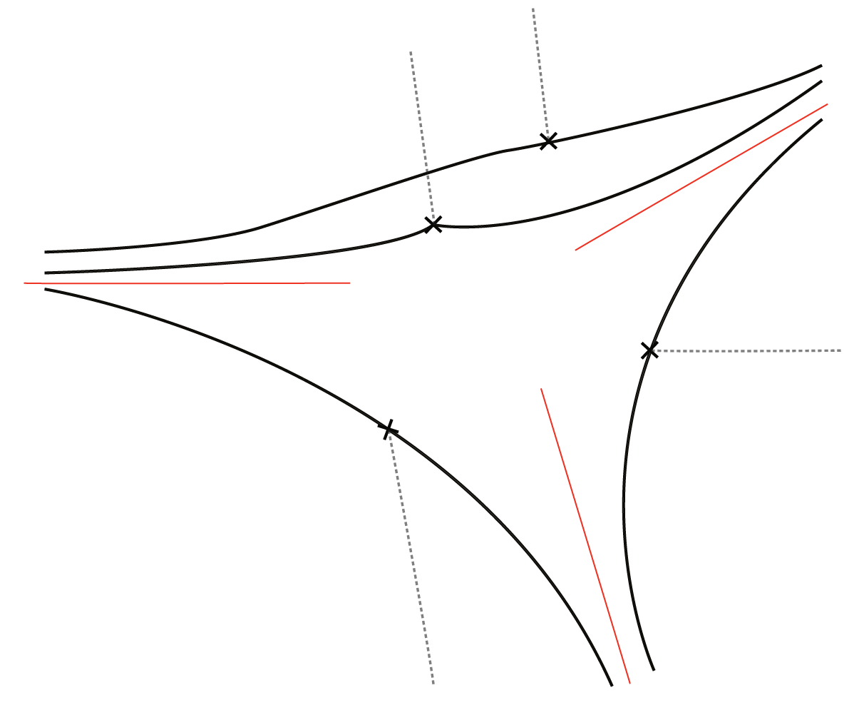
Figure 1. The lines are in solid black. The slopes of red rays and the eigenrays are cyclically ordered with respect to the cyclic order at infinity, where the slopes of consecutive a red ray and eigenray are not equal.

1.3.2. Relation with Family Floer theory

Let us also make a comparison with Family Floer theory. Starting with $\pi_{\mathcal{R}}:M_{\mathcal{R}}\to B_{\mathcal{R}}$, Hang Yuan constructs a rigid analytic space $\mathcal{Z}$ with an analytic torus fibration $\mathcal{Z}\to B_{\mathcal{R}}^{reg}$ in [31, Theorem 1.3].

Conjecture 1.11.

$\mathcal{Z}$ is isomorphic as a rigid analytic space to $p_{\mathcal{R}}^{-1}(B_{\mathcal{R}}^{reg})$ in a fiber preserving way.

A conceptual proof of this conjecture would involve setting up closed-open string maps that realize the idea that sections of the sheaf $\mathcal{F}_{\mathcal{R}}$ give rise to functions on the Family Floer mirror.

1.3.3. Further expectations for closed string invariants

Let’s continue with closed string consequences. The first step to this is to extend the local computations to show that there is an isomorphism of algebras

(2) $$SH^{*}_{M_{\mathcal{R}}}(\pi^{-1}(P);\Lambda)\to\Lambda^{*}Der(\mathcal{F}_{\mathcal{R}}(P),\mathcal{F}_{\mathcal{R}}(P)),$$

whenever $P$ is a small admissible polygon. We proved this when $P$ does not contain a node in this paper. We are also confident that this is true when $P$ does not contain a node with multiplicity more than $1$. Otherwise we do not know the answer.

Remark 1.12.

An element $a\in SH^{1}_{M}(K)$ defines the derivation $[a,\cdot]$ on $SH^{0}_{M}(K)$, so at least in degree $1$ the map can be defined naturally.

Recall that given compact subsets $P_{1},\ldots,P_{n}$ of $B_{\mathcal{R}}$, we have a convergent spectral sequence:

(3) $$\bigoplus_{0\neq I\subset[n],|I|=p}SH_{M}^{q}\left(\bigcap_{i\in I}\pi^{-1}(P_{i})\right)\Rightarrow SH_{M}^{p+q}\left(\bigcup_{i=1}^{n}\pi^{-1}(P_{i})\right).$$

The differentials in the first page of the spectral sequence are precisely the Cech differentials. We believe that it is reasonable to conjecture that the spectral sequence degenerates after that page when $P_{i}$ are small admissible polygons. This would allow us to conclude the first part of the following.

Conjecture 1.13.

If the multiplicites of nodes in $\mathcal{R}$ are all $1$, there exists a ring isomorphism

$$SH_{M_{\mathcal{R}}}^{k}(M_{\mathcal{R}},\Lambda)\to\bigoplus_{p+q=k}H^{p}(\mathcal{Y}_{\mathcal{R}},\Lambda^{q}T\mathcal{Y}_{\mathcal{R}}),$$

where the right hand is the Cech cohomology with respect to the defining affinoid cover.

Using $\Omega_{\mathcal{R}}$ we equip the polyvector fields with a differential by transporting the deRham differential. This differential is compatible with the BV operator.

Remark 1.14.

It is not difficult to see that $\pi_{\mathcal{R}}$ always has a Lagrangian section, in fact one that is the fixed point set of an anti-symplectic involution [4]. Let us call its image $L$. Assuming that all multiplicities of nodes are $1$ and $P\subset B$ is a small admissible polygon, we conjecture that the local generation criterion is satisfied at $K=\pi^{-1}(P),$ namely the open-closed map

$$HH_{2}(CF_{M_{\mathcal{R}}}^{*}(K;L;\Lambda))\to SH_{M_{\mathcal{R}}}^{0}(K;\Lambda)$$

hits the unit.

Another conjecture is that our locality results (based on the existence of complete embeddings) holds for $HF_{M_{\mathcal{R}}}^{*}(\pi^{-1}(P);L;\Lambda)$ as well and imply that it is supported in degree $0$. Then, we would obtain that the closed open map is an isomorphism

$$SH_{M_{\mathcal{R}}}^{*}(\pi^{-1}(P);\Lambda)\to HH^{*}(HF_{M_{\mathcal{R}}}^{0}(\pi^{-1}(P);L;\Lambda)).$$

Using commutativity of $HF_{M_{\mathcal{R}}}^{0}(L;\pi^{-1}(P);\Lambda)$ and HKR, we get the isomorphism from (2).

We expect that the mentioned degeneration at the $E_{2}$ page of the spectral sequence in (3) would follow from the construction of a chain level closed-open map (which is a quasi-isomorphism by the local generation criterion) and the chain level lift of HKR. Assuming that the closed open map and HKR respect the $BV_{\infty}$ structures in a suitable way, the comparison between the $BV$-operator and the deRham differential is also a direct consequence of local generation and HKR.

1.3.4. Homological mirror symmetry

In terms of open string mirror symmetry we expect

Conjecture 1.15.

There exists a canonical $A_{\infty}$-functor

$$Fuk(M_{\mathcal{R}})\to Coh_{dg}(\mathcal{Y_{\mathcal{R}}}).$$

If we assume that multiplicities of nodes are all $1$, it is a quasi-equivalence.

Let us also briefly mention the approach to Conjecture 1.15. Here we are omitting any discussion of the serious question of what we mean by $Fuk(M_{\mathcal{R}})$. Let $L$ be as in Remark 1.14 and assume that the mirror $\mathcal{Y}_{\mathcal{R}}$ is equivalently constructed using the relative Lagrangian Floer homology of $L$ as suggested by the discussion in Remark 1.14. To construct the functor we send each Lagrangian $L^{\prime}$ to the complex of $\mathcal{O}$-modules $CF_{M_{\mathcal{R}}}^{*}(\pi_{\mathcal{R}}^{-1}(P);L,L^{\prime};\Lambda)$. Coherence will follow from the local generation property of $L$, using the unitality of restriction maps. On morphisms, we use the product

$$CF_{M_{\mathcal{R}}}^{*}(K;L,L_{1};\Lambda)\otimes CF_{M_{\mathcal{R}}}^{*}(K;L_{1},L_{2};\Lambda)\to CF_{M_{\mathcal{R}}}^{*}(K;L,L_{2};\Lambda)$$

and so on for higher terms of the morphisms. Finally, a version of the local-to-global property will allow us to deduce the full and faithfulness of the functor from the local generation of $L$.

Essential surjectivity is less clear and here we believe it would follow from specific results in this case inspired by Hacking-Keating homological mirror symmetry [11], which we now turn to – in general there is no reason to expect essential surjectivity.

1.3.5. Relation with Hacking-Keating mirror symmetry

It is possible to understand the mirror in Theorem 1.1 concretely in general, not just in the local version. Namely, we strongly believe that it is the (rigid analytification of the) interior of a log CY surface defined over the Novikov field.

Let us be more precise. One can isotope $\mathcal{R}$ through eigenray diagrams with the same number of nodes into an exact eigenray diagram $\mathcal{R}^{\prime}$. To each node $n$ of $\mathcal{R}^{\prime}$ we can associate a real number

$$x_{n}:=m_{n}(\Delta_{n}\times v_{n})$$

where $m_{n}$ is the multiplicity, $\Delta_{n}$ is the displacement vector and $v_{n}$ is the primitive integral vector along the eigenray of $n$.

We now think of the rays of $\mathcal{R}^{\prime}$ as forming a fan defining the toric variety $V_{\mathcal{R}}$ over $\Lambda$. By construction we can choose an identification of each one dimensional toric orbit with $\Lambda^{*}$ (uniquely up to an overall action by element of the two dimensional torus). We then do one Kaliman modification for each node on the corresponding irreducible toric divisor of $V_{\mathcal{R}}$ at the point $T^{x_{n}}$. We denote by $Y_{\mathcal{R}}$ the resulting non-proper scheme over $\Lambda$.

Conjecture 1.16.

$\mathcal{Y}_{\mathcal{R}}$ is the analytification of $Y_{\mathcal{R}}$.

In Section 7.7 of [9], we gave another description of $Y_{\mathcal{R}}$ by gluing certain affine schemes, which is the one that would actually be useful in the proof. The proof also requires a Zariski analogue of [28] to justify this gluing construction, which is actually straightforward.

In the case, where $\mathcal{R}$ is exact and we use $\mathbb{C}$ as our base field, our $M_{\mathcal{R}}$ is precisely the $A$-side and $Y_{\mathcal{R}}$ is the base change of the $B$-side of Hacking-Keating’s [11, Theorem 1.1].

1.4. Outline

In Section 2, we give a brief account of eigenray diagrams and nodal integral affine manifolds, in particular of their $G$-topology. Section 3 is where we discuss the $B$-side local models $Y_{k}^{an}$ and their extra structures. In Section 4, we go over some generalities regarding relative symplectic cohomology and its relation to symplectic cohomology of Liouville manifolds. In Section 5, we compute the relative symplectic cohomology presheaf in the base of $T^{*}T^{n}\to\mathbb{R}^{n}$ in all degrees relying on Viterbo’s theorem. We then go on to the proof of Theorem 1.8, which takes up the next four sections. In Section 6, we construct sheaf isomorphisms between $\mathcal{O}_{k}$ and $\mathcal{F}_{k}$ in the complement of each of the eigenrays. In the next section, Section 7, we prove a slight extension of our locality for complete embeddings result showing that the locality isomorphisms for different complete embeddings are the same in the zeroth order. Section 8 is where we finish the computation of $A$-side wall-crossing. In the final section of local computations, Section 9, we extend the isomorphism of $\mathcal{O}_{k}$ and $\mathcal{F}_{k}$ from the punctured plane to the entire plane by proving an $A$-side Hartogs extension theorem for relative symplectic cohomology in degree $0$. In Section 10, we first prove Theorem 1.5 relying on the locality for complete embeddings theorem and the local results. Then we go on to prove our main result Theorem 1.1 using the properties listed in Theorem 1.5. We end our paper with a short section that discusses some higher dimensional situations to which our methods extend straightforwardly.

Acknowledgements

Y.G. was supported by the ISF (grant no. 2445/20). U.V. was supported by the TÜBİTAK 2236 (CoCirc2) programme with a grant numbered 121C034.

2. Some integral affine geometry

2.1. Local models

Let us denote by $B_{0}^{n}$ the Euclidean space $\mathbb{R}^{n}$ as an integral affine manifold with its standard integral affine structure. We abbreviate $B_{0}:=B_{0}^{2}$.

For $k>0$ and primitive vector $e\in\mathbb{Z}^{2}$, consider the linear map $A_{k,e}:\mathbb{R}^{2}\to\mathbb{R}^{2}$ defined by

(4) $$v\mapsto v-k\cdot det(e,v)\cdot e.$$

We define the integral affine manifold $B_{k,e}^{reg}$ by gluing

$$B_{e}^{+}:=\mathbb{R}^{2}\setminus\{c\cdot e\mid c\geq 0\}\subset B_{0}\text{ and }B_{e}^{-}:=\mathbb{R}^{2}\setminus\{c\cdot e\mid c\leq 0\}\subset B_{0}$$

with the gluing map $\phi:B_{e}^{+}\cap B_{e}^{-}\to B_{e}^{+}\cap B_{e}^{-}$ from $B_{e}^{-}$ to $B_{e}^{+}$ defined by

$$\phi(w)=\begin{cases}w,&det(e,w)>0\\ A_{k,e}^{-1}(w),&det(e,w)<0.\end{cases}$$

Notice that we can replace $B_{e}^{-}$ with an arbitrary neighborhood of $\{c\cdot e\mid c>0\}$ inside $\mathbb{R}^{2}$ disjoint from $\{c\cdot e\mid c\leq 0\}.$ For convenience, when $e=e_{1}$ is the first standard basis vector we simply omit the subscript $e$’s and write $B_{k}^{reg}$. Clearly $B_{k,e}^{reg}$ is integral affine isomorphic to $B_{k}^{reg}$ but this involves choices and we prefer to not identify them.

Note that $B_{k,e}^{reg}$ can be embedded into $\mathbb{R}^{2}$ as a $PL$-manifold by the map that sends $B_{e}^{+}$ to $B_{e}^{+}$ with the identity map. We define $B_{k,e}$ as the $PL$-manifold $\mathbb{R}^{2}$ along with the integral affine structure on $\mathbb{R}^{2}\setminus\{0\}$ induced from this embedding. Let $B_{0,e}^{reg}:=B_{0,e}:=B_{0}$. Let us denote the canonical embeddings $B_{e}^{\pm}\to B_{k,e}$ by $E^{\pm}_{k}$. When $e=e_{1}$, we omit it from notation.

Inside $B_{k,e}$, we define

• a rational line to be the image of a complete affine geodesic $\mathbb{R}\to B_{k,e}^{reg}$ with rational slope.

• a rational halfspace to be the closure of a connected component of $B_{k,e}\setminus l$ with $l$ a rational line.

• an admissible convex polygon to be a compact subset that is a finite intersection of rational halfspaces.

We can similarly define admissible convex polytopes on $B_{0}^{n}$ as well. We omit spelling this out. This is the same notion as $\mathbb{R}$-rational convex polyhedra from [6, Convention 1.3].

2.2. Eigenray diagrams

A ray in $\mathbb{R}^{2}$ is the image of a map of the form $[0,\infty)\to\mathbb{R}^{2}$, $t\mapsto x+vt$, where $x,v\in\mathbb{R}^{2}$. Let us define an eigenray diagram $\mathcal{R}$ to consist of the following data:

1. A finite set of pairwise disjoint rays $l_{i}$, $i=1,\ldots,k,$ in ${\mathbb{R}}^{2}$ with rational slopes.

2. A finite set of points on each ray including the starting point. Let us call the set of all of them $N_{\mathcal{R}}$.

3. A map $m_{\mathcal{R}}:N_{\mathcal{R}}\to\mathbb{Z}_{\geq 1}$.

An eigenray diagram can be equivalently described by the finite multiset $\{\underbrace{l^{n},\ldots,l^{n}}_{m_{R}(n)}\}_{n\in N_{\mathcal{R}}}$, which is a finite multiset of rays with rational slopes any two of which are either disjoint or so that one is contained in the other. A node removal from an eigenray diagram $\mathcal{R}$ means removing an element of this multiset.

Each eigenray diagram $\mathcal{R}$ gives rise to a nodal integral affine manifold $B_{\mathcal{R}}$ with a preferred $PL$ homeomorphism $\psi_{\mathcal{R}}:\mathbb{R}^{2}\to B_{\mathcal{R}}$ such that

• $\psi_{\mathcal{R}}(N_{\mathcal{R}})$ is the set of nodes of $B_{\mathcal{R}}$

• $\psi_{\mathcal{R}}$ restricted to the complement of the rays in $\mathcal{R}$ is an integral affine isomorphism onto its image.

• The multiplicity of a node $\psi_{\mathcal{R}}(n)$ is $m_{\mathcal{R}}(n)$.

• For any $n\in N_{\mathcal{R}}$, $\psi_{\mathcal{R}}(l^{n})$ is a monodromy invariant ray of $\psi_{\mathcal{R}}(n)$.

The construction involves starting with the standard integral affine $\mathbb{R}^{2}$ and doing a modification similar to the one in the definition of $B_{k,e}$ for each element $n$ of $N_{\mathcal{R}}$ by removing $l_{n}$ and then re-gluing an arbitrarily small product neighborhood of $l_{n}$. The order in which these surgeries are made does not change the resulting nodal integral affine manifold. For details see [9, Section 7].

We will now define a $G$-topology on $B_{\mathcal{R}}$. For the purposes of this paper a $G$-topology on a set $X$ is a set $\mathfrak{U}$ of subsets $U\subset X$ and a set of set-theoretic coverings $Cov(\mathfrak{U})$ of each $U\in\mathfrak{U}$ by collections of members of $\mathfrak{U}$ such that

1. $\varnothing\in\mathfrak{U}$,

2. $\{U\}\in Cov(U)$ for all $U\in\mathfrak{U}$

3. $\mathfrak{U}$ is stable under finite intersections

4. if $\{U_{i}\}\in Cov(U)$ and $V\subset U$ then $V\in\mathfrak{U}$ if and only if $V\cap U_{i}\in\mathfrak{U}$ for all $i$

5. if $\{V_{ij}\}_{j\in J_{i}}\in Cov(U_{i})$ for $\{U_{i}\}\in Cov(U)$ then $\{V_{ij}\}_{i,j}\in Cov(U)$.

An admissible convex polygon inside $B_{\mathcal{R}}$ is a subset that is the image of an admissible convex polygon inside some open subset $U\subset B_{k}$ under an embedding $U\to B_{\mathcal{R}}$ of nodal integral affine manifolds. A finite (possibly empty) union of admissible convex polygons is called an admissible polygon. An admissible covering is any finite covering by admissible polygons. We define a $G$-topology on $B_{\mathcal{R}}$ whose opens are the admissible polygons and whose allowed covers are the admissible covers. From now on we consider $\mathcal{F}(\cdot):=SH^{0}_{M_{\mathcal{R}}}(\pi_{\mathcal{R}}^{-1}(\cdot);\Lambda)$ as a sheaf over this $G$-topology, and denote it by $\mathcal{F}_{\mathcal{R}}$.

Let $l_{1},\ldots,l_{n}$ be the rays of $\mathcal{R}$. Let us call an admissible convex polygon a small admissible polygon if, for some $i,j$, it intersects $\psi_{\mathcal{R}}(l_{i})$ and $\psi_{\mathcal{R}}(l_{j}),$ then $l_{i}$ and $l_{j}$ are not disjoint. We can also talk about a $G$-topology on $B_{\mathcal{R}}$ of small admissible polygons and finite covers by small admissible polygons, but we will not do this to not create confusion.

Lemma 2.1.

Let $\mathcal{G}$ and $\mathcal{G}^{\prime}$ be two sheaves of $\Lambda$-algebras on the $G$-topology of $B_{\mathcal{R}}$. Assume that we are given isomorphisms of algebras

$$\mathcal{G}(P)\to\mathcal{G}^{\prime}(P)$$

for every small admissible polygon $P$, which are compatible with restriction maps. Then, there is a unique isomorphism of sheaves of $\Lambda$-algebras $\mathcal{G}\to\mathcal{G}^{\prime}$ extending the given isomorphisms.

Remark 2.2.

The notion of a small admissible polygon is an ad-hoc notion that depends on the eigenray diagram presentation of the nodal integral manifold $B_{\mathcal{R}}$.

3. Local models from non-archimedean geometry

3.1. Analytification of $(\Bbbk^{*})^{n}$ and the tropicalization map

Let $\Bbbk$ be an algebraically closed non-archimedean field whose valuation map surjects onto $\mathbb{R}\cup\{\infty\}$.

Let us define $\mathcal{Y}_{0}^{n}$ to be the rigid analytification (see [3, Section 5.4]) of the affine variety $Spec(\Bbbk[(\mathbb{Z}^{n})^{\vee}])$. As a set $\mathcal{Y}_{0}^{n}$ is canonically identified with the closed points of $Spec(\Bbbk[(\mathbb{Z}^{n})^{\vee}])$ (see [3, Proposition 4]), which we can in turn canonically identify with $(\Bbbk^{*})^{n}$ using the standard basis of $\mathbb{Z}^{n}$ (and its dual). Define the tropicalization map $p_{0}:\mathcal{Y}_{0}^{n}\to B_{0}^{n}=\mathbb{R}^{n}$ via

$$(y_{1},\ldots,y_{n})\mapsto(val(y_{1}),\ldots,val(y_{n})).$$

Proposition 3.1.

Let $P\subset B_{0}^{n}$ be an admissible convex polytope. Then

1. $p_{0}^{-1}(P)\subset\mathcal{Y}_{0}^{n}$ is an affinoid domain.

2. $\mathcal{O}(p_{0}^{-1}(P))$ is the completion of $\Bbbk[(\mathbb{Z}^{n})^{\vee}]$ with respect to the valuation

   (5) $$val_{P}(f=\sum a_{j}x^{j}):=\inf_{m\in P}\inf_{j}\left(val(a_{j})+j(m)\right).$$

3. If $Q\subset P$ is also an admissible convex polytope, then

   $$p_{0}^{-1}(Q)\subset p_{0}^{-1}(P)$$

   is a Weierstrass (and in particular affinoid) subdomain.

Proof.

These statements are well-known, see e.g. [6, Section 3] and [10, Section 4]. ∎

Let us explain part (2) a little more concretely. We introduce the vector space of formal Luarent power series

$$\Bbbk[[(\mathbb{Z}^{n})^{\vee}]].$$

To be explicit, these are collections of coefficients $a_{j}$ indexed by $j\in(\mathbb{Z}^{n})^{\vee}$ which we write as $\sum a_{j}x^{j}$. Note that we do not have a well defined multiplication operation here. We say that a formal sum $\sum a_{j}x^{j}$ converges at a point $m\in B_{0}^{n}$, if for every real number $R$, there are only finitely many $j\in(\mathbb{Z}^{n})^{\vee}$ such that $val(a_{j})+j(m))<R$.

To any admissible convex polytope $P\subset B_{0}^{n}$ and $f\in\mathcal{O}(p_{0}^{-1}(P))$, we can canonically associate a formal Laurent power series, in other words we have a canonical injection

$$\mathcal{O}(p_{0}^{-1}(P))\to\Bbbk[[(\mathbb{Z}^{n})^{\vee}]].$$

The image of this map is precisely the formal Laurent power series which converge on $P$. From now on we call this image the formal expression of an element of $\mathcal{O}(p_{0}^{-1}(P))$

Let us define a sheaf $\mathcal{O}_{0}$ on the $G$-topology of $B_{0}^{n}$ by first setting

$$\mathcal{O}_{0}(P):=\mathcal{O}(p_{0}^{-1}(P))$$

on an admissible convex polytope $P$ and then defining $\mathcal{O}_{0}(\cup P_{i})$ as the equalizer

(6)

for admissible convex polytopes $P_{1},\ldots,P_{k}$.

Tate’s acyclicity theorem guarantees that this indeed defines the desired sheaf. We of course have $(p_{0})_{*}\mathcal{O}=\mathcal{O}_{0}$ but we chose to be more concrete for once.

Proposition 3.2.

Let $P_{1},\ldots,P_{k}$ be admissible convex polytopes in $B_{0}^{n}$. Assume that $\cup P_{i}$ is connected and the convex hull $P$ of $\cup P_{i}$ is an admissible convex polytope, then the canonical map

$$\mathcal{O}_{0}(P)\to\mathcal{O}_{0}(\cup P_{i})$$

is an isomorphism.

Proof.

We identify each function with its formal expression. Because of the connectedness assumption $\mathcal{O}_{0}(\cup P_{i})$ is simply a single element of $\Bbbk[[(\mathbb{Z}^{n})^{\vee}]]$ which converges at all points of $\cup P_{i}$. It is clear that a formal expression converges at two points of $B_{0}^{n}$ if and only if it converges at all points lying along the affine line segment that connects these two points. This finishes the proof. ∎

Remark 3.3.

This proposition is related to results from the theory of several complex variables which relate the holomorphic convex hulls with usual convex hulls. Since this is a much simpler result explaining the connection seems pointless.

Let $H$ be co-oriented rational hyperplane in $B_{0}^{n}$. Denote by $l_{H}\in(\mathbb{Z}^{n})^{\vee}$ be the positive (with respect to the co-orientation) primitive generator of the annihilator of the vectors tangent to $H$. Then

(7) $$x^{l_{H}}\in\Bbbk[(\mathbb{Z}^{n})^{\vee}]$$

defines an element of each $\mathcal{O}_{0}(P)$, where $P$ is an admissible polytope. The formal expression of $x^{l_{H}}$ is independent of $P$ and is nothing but $x^{l_{H}}\in\Bbbk[[(\mathbb{Z}^{n})^{\vee}]].$

Given a hyperplane $H$ and a subset $S$ intersecting exactly one of the components of $B_{0}^{n}\setminus H$ we refer to the coorientation for which $l_{H}$ increases as go towards the side containing $S$, the $S$-co-orientation.

To orient the reader let us work out an example. Let $P$ be the triangle with vertices in $(0,0),(1,0),(0,1)$. Let $H$ be the line containing the hypotenuse of $P$ with its $P$-co-orientation. Let $e_{1}^{\vee}$ and $e_{2}^{\vee}$ be the standard basis of $(\mathbb{Z}^{2})^{\vee}$ and let $z_{i}:=x^{e_{i}^{\vee}}$ for $i=1,2$. Then

$$x^{l_{H}}=z_{1}^{-1}z_{2}^{-1}.$$

The following is a version of the uniqueness of analytic continuation.

Proposition 3.4.

Assume that $P\subset Q\subset B_{0}^{n}$ are admissible polytopes and let $Q$ be connected. Then, the restriction map $\mathcal{O}_{0}(Q)\to\mathcal{O}_{0}(P)$ is injective.

Consider the nowhere vanishing analytic volume form

$$\Omega_{0}:=\frac{dy_{1}}{y_{1}}\wedge\ldots\wedge\frac{dy_{n}}{y_{n}}$$

on $\mathcal{Y}^{n}_{0}$. Let $\mathcal{T}^{*}_{\mathcal{Y}^{n}_{0}}$ be the sheaf of polyvector fields on $\mathcal{Y}^{n}_{0}$. An easy computation shows that for $P$ an admissible convex polygon we have an isomorphism of graded normed algebras

(8) $$\mathcal{T}^{*}_{\mathcal{Y}^{n}_{0}}(p_{0}^{-1}(P))\simeq\mathcal{O}_{0}(P)[\partial_{1},\ldots,\partial_{n}]$$

where the degree $1$ super-commutative variables $\partial_{i}$ correspond to the valuation zero derivations $y_{i}\frac{\partial}{\partial y_{i}}.$

Observe that $\Omega_{0}$ gives rise to a degree reversing isomorphism, $i_{\Omega_{0}}:\Omega^{*}_{\mathcal{Y}^{n}_{0}}\to\mathcal{T}^{n-*}_{\mathcal{Y}^{n}_{0}}$, between the poly-vector fields and the differential forms. We denote by $div_{\Omega_{0}}:\mathcal{T}^{*}_{\mathcal{Y}^{n}_{0}}\to\mathcal{T}^{*+1}_{\mathcal{Y}^{n}_{0}}$ the degree $1$ operator on given by

(9) $$div_{\Omega_{0}}\omega:=(-1)^{|\omega|}\Omega_{0}\circ d\circ\Omega_{0}^{-1}\omega$$

for a homogeneous $\omega$, where $d$ is the exterior derivative. A basic observation is that $(\mathcal{T}^{*}_{\mathcal{Y}^{n}_{0}},div_{\Omega_{0}})$ is a sheaf of BV algebras (see [1, Section 2.1] with the sign correction from [18, Section 5]). We thus obtain a sheaf of BV algebras on the $G$-topology of $B_{0}^{n}$ given by

$$\mathcal{A}^{*}(P):=\left(\mathcal{T}^{*}_{\mathcal{Y}^{n}_{0}}(p_{0}^{-1}(P)),div_{\Omega_{0}}\right).$$

Proposition 3.5.

Consider an isomorphism of unital BV algebras $f^{*}:\mathcal{A}^{*}(P)\to\mathcal{A}^{*}(P^{\prime})$ with $P$ and $P^{\prime}$ convex admissible polytopes in $B_{0}^{n}$. Then, the map

$$(f^{0})_{*}:\Omega^{n}A^{0}(P)\to\Omega^{n}A^{0}(P^{\prime})$$

sends $\Omega_{0}$ to $c\Omega_{0}$, for some $c\in\Bbbk^{*}.$

Proof.

We have two maps

(10) $$(f^{0})_{*}\text{ and }g=i_{\Omega_{0}}^{-1}\circ f\circ i_{\Omega_{0}}:\Omega^{*}A^{0}(P)\to\Omega^{*}A^{0}(P^{\prime}).$$

Considering $\Omega^{*}A^{0}(P^{\prime})$ as an $A^{0}(P)$ module where $a$ acts by multiplication with $f^{0}(a)$, we see that both of these are maps of $A^{0}(P)$ modules. In addition, both maps are chain maps with respect to the exterior derivative.

Note that $g(1)$ has to be a non-zero closed element, i.e. an element $c\in\Bbbk^{*}$. Then we immediately see that $g$ restricted to $A^{0}(P)$ equals $cf^{0}$ for $c=g(1)$. Observe that $\Omega^{k}A^{0}(P)$ for $k\geq 1$ is generated as an $A^{0}(P)$ module by the forms $dy^{I}$ for $|I|=k$. Each of these generators is exact. From this we deduce inductively that $g=c(f^{0})_{*}$ in all degrees.

Finally, note that $g\Omega_{0}=\Omega_{0}$ since $i_{\Omega_{0}}(\Omega_{0})=1$. The claim follows

∎

3.2. Analytification of $Y_{k}$

Let us now consider the affine variety

$$Y_{k}=Spec(\Bbbk[x,y,u^{\pm}]/(xy-(u+1)^{k}),$$

for $k\geq 1$ and its rigid analytification $Y_{k}^{an}$. Note that $Y_{k}$ is smooth if and only if $k=1$. On the other hand $Y_{k}$ is normal for all $k\geq 1$ as it is an open subset of a surface $\{f=0\}\subset\mathbb{C}^{3}$ with only isolated singularities. As a set

$$Y_{k}^{an}=M(\Bbbk[x,y,u^{\pm}]/(xy-(u+1)^{k}).$$

In this section we prove that $Y_{k}^{an}$ admits a Stein continuous map $p_{k}$ to $B_{k}$, which induces the integral affine structure of Section 2.1 on $B_{k}^{reg}$. In particular all points other than the origin are regular. The notion of an integral affine structure induced by a continuous map as above is explained in [13, Theorem 1]. This section is based on Section 8 of [13].

Remark 3.6.

Suitably interpreted the constructions extend to the $k=0$ case and recover the previous section in dimension $2$.

The rigid analytic space $Y_{k}^{an}$ is embedded inside the analytification of $\mathbb{A}^{2}_{\Bbbk}\times\Bbbk^{*}$ as a set by functoriality of analytification. We consider the map

(11) $$((x,y,u)\mapsto(\min{(0,val(x))},\min{(0,val(y))},val(u)).$$

The restriction of this map to $Y_{k}^{an}$ defines a map

$$p_{k}:Y_{k}^{an}\to\mathbb{R}^{3}.$$

Remark 3.7.

Note that we have a map $\mathbb{A}_{\Bbbk}^{1}\to\mathbb{R}\cup\{\infty\}$ which sends each element to its valuation. Just to orient ourselves this map sends $1$ to $0$ and $0$ to $\infty$. The maps in the Equation 11 obtained by composing this map with the map that collapses $\mathbb{R}\cup\{\infty\}$ to $\mathbb{R}_{\leq 0}$ in the non-negative side. Now the entire ball of radius $1$ (and nothing else), including $0$ and $1$, map to $0$. Here the ball is defined with respect to the norm given by $e^{-\operatorname{val}}$.

Let us consider a copy of $(\Bbbk^{*})^{2}$ with coordinates $\xi^{+},\eta^{+}$. We have the tropicalization map $p_{0}:(\Bbbk^{*})^{2}\to\mathbb{R}^{2}$ given by $(\xi^{+},\eta^{+})\mapsto(v^{+},u^{+})=(val(\xi^{+}),val(\eta^{+}))$. Let $B^{+}$ be the complement of the ray $\{(v^{+},0)\mid v^{+}\geq 0\}$ in $\mathbb{R}^{2}$, and let $T^{+}$ be the preimage of $B^{+}$ under the tropicalization map.

Define an embedding

$$g^{+}:(\Bbbk^{*})^{2}\to Y_{k}^{an}$$

by

$$x\mapsto\xi^{+},y\mapsto\frac{1}{\xi^{+}}\left(1+\eta^{+}\right)^{k}\text{ and }u\mapsto\eta^{+}.$$

We can restrict this embedding to $T^{+}$. There then exists a map $f^{+}:B^{+}\to\mathbb{R}^{3}$ fitting into the diagram

(16) $$\lx@xy@svg{\hbox{\raise 0.0pt\hbox{\kern 11.52188pt\hbox{\ignorespaces\ignorespaces\ignorespaces\hbox{\vtop{\kern 0.0pt\offinterlineskip\halign{\entry@#!@&&\entry@@#!@\cr&\\&\crcr}}}\ignorespaces{\hbox{\kern-8.7941pt\raise 0.0pt\hbox{\hbox{\kern 0.0pt\raise 0.0pt\hbox{\hbox{\kern 3.0pt\raise 0.0pt\hbox{$\textstyle{T^{+}\ignorespaces\ignorespaces\ignorespaces\ignorespaces\ignorespaces\ignorespaces\ignorespaces\ignorespaces}$}}}}}}}\ignorespaces\ignorespaces\ignorespaces\ignorespaces{}{\hbox{\lx@xy@droprule}}\ignorespaces\ignorespaces\ignorespaces{\hbox{\kern-11.52188pt\raise-19.7622pt\hbox{{}\hbox{\kern 0.0pt\raise 0.0pt\hbox{\hbox{\kern 3.0pt\hbox{\hbox{\kern 0.0pt\raise-0.8264pt\hbox{$\scriptstyle{p_{0}}$}}}\kern 3.0pt}}}}}}\ignorespaces{\hbox{\kern 0.0pt\raise-28.05777pt\hbox{\hbox{\kern 0.0pt\raise 0.0pt\hbox{\lx@xy@tip{1}\lx@xy@tip{-1}}}}}}{\hbox{\lx@xy@droprule}}{\hbox{\lx@xy@droprule}}\ignorespaces\ignorespaces\ignorespaces\ignorespaces{}{\hbox{\lx@xy@droprule}}\ignorespaces\ignorespaces\ignorespaces{\hbox{\kern 14.53993pt\raise 5.77083pt\hbox{{}\hbox{\kern 0.0pt\raise 0.0pt\hbox{\hbox{\kern 3.0pt\hbox{\hbox{\kern 0.0pt\raise-1.40973pt\hbox{$\scriptstyle{g^{+}}$}}}\kern 3.0pt}}}}}}\ignorespaces{\hbox{\kern 33.22118pt\raise 0.0pt\hbox{\hbox{\kern 0.0pt\raise 0.0pt\hbox{\lx@xy@tip{1}\lx@xy@tip{-1}}}}}}{\hbox{\lx@xy@droprule}}{\hbox{\lx@xy@droprule}}{\hbox{\kern 33.22118pt\raise 0.0pt\hbox{\hbox{\kern 0.0pt\raise 0.0pt\hbox{\hbox{\kern 3.0pt\raise 0.0pt\hbox{$\textstyle{Y_{k}^{an}\ignorespaces\ignorespaces\ignorespaces\ignorespaces}$}}}}}}}\ignorespaces\ignorespaces\ignorespaces\ignorespaces{}{\hbox{\lx@xy@droprule}}\ignorespaces\ignorespaces\ignorespaces{\hbox{\kern 41.7809pt\raise-19.7622pt\hbox{{}\hbox{\kern 0.0pt\raise 0.0pt\hbox{\hbox{\kern 3.0pt\hbox{\hbox{\kern 0.0pt\raise-0.8125pt\hbox{$\scriptstyle{p_{k}}$}}}\kern 3.0pt}}}}}}\ignorespaces{\hbox{\kern 41.7809pt\raise-27.88666pt\hbox{\hbox{\kern 0.0pt\raise 0.0pt\hbox{\lx@xy@tip{1}\lx@xy@tip{-1}}}}}}{\hbox{\lx@xy@droprule}}{\hbox{\lx@xy@droprule}}{\hbox{\kern-9.22118pt\raise-39.52441pt\hbox{\hbox{\kern 0.0pt\raise 0.0pt\hbox{\hbox{\kern 3.0pt\raise 0.0pt\hbox{$\textstyle{B^{+}\ignorespaces\ignorespaces\ignorespaces\ignorespaces}$}}}}}}}\ignorespaces\ignorespaces\ignorespaces\ignorespaces{}{\hbox{\lx@xy@droprule}}\ignorespaces\ignorespaces\ignorespaces{\hbox{\kern 14.2446pt\raise-32.82999pt\hbox{{}\hbox{\kern 0.0pt\raise 0.0pt\hbox{\hbox{\kern 3.0pt\hbox{\hbox{\kern 0.0pt\raise-2.33333pt\hbox{$\scriptstyle{f^{+}}$}}}\kern 3.0pt}}}}}}\ignorespaces{\hbox{\kern 33.70035pt\raise-39.52441pt\hbox{\hbox{\kern 0.0pt\raise 0.0pt\hbox{\lx@xy@tip{1}\lx@xy@tip{-1}}}}}}{\hbox{\lx@xy@droprule}}{\hbox{\lx@xy@droprule}}{\hbox{\kern 33.70035pt\raise-39.52441pt\hbox{\hbox{\kern 0.0pt\raise 0.0pt\hbox{\hbox{\kern 3.0pt\raise 0.0pt\hbox{$\textstyle{\mathbb{R}^{3}}$}}}}}}}\ignorespaces}}}}\ignorespaces. \textstyle{T^{+}\ignorespaces\ignorespaces\ignorespaces\ignorespaces\ignorespaces\ignorespaces\ignorespaces\ignorespaces} \scriptstyle{p_{0}} \scriptstyle{g^{+}} \textstyle{Y_{k}^{an}\ignorespaces\ignorespaces\ignorespaces\ignorespaces} \scriptstyle{p_{k}} \textstyle{B^{+}\ignorespaces\ignorespaces\ignorespaces\ignorespaces} \scriptstyle{f^{+}} \textstyle{\mathbb{R}^{3}} \textstyle{T^{+}\ignorespaces\ignorespaces\ignorespaces\ignorespaces\ignorespaces\ignorespaces\ignorespaces\ignorespaces} \scriptstyle{p_{0}} \scriptstyle{g^{+}} \textstyle{Y_{k}^{an}\ignorespaces\ignorespaces\ignorespaces\ignorespaces} \scriptstyle{p_{k}} \textstyle{B^{+}\ignorespaces\ignorespaces\ignorespaces\ignorespaces} \scriptstyle{f^{+}} \textstyle{\mathbb{R}^{3}}$$

$f^{+}$ can be computed explicitly:

Proposition 3.8.

$$f^{+}(v^{+},u^{+})=\begin{cases}\left(v^{+},\min{(0,ku^{+}-v^{+})},u^{+}\right),&\qquad v^{+}\leq 0\\ \left(0,-v^{+}+\min{(ku^{+},0)},u^{+}\right),&\qquad v^{+}\geq 0.\end{cases}$$

Proof.

To see this substitute $\operatorname{val}(y)=\begin{cases}ku^{+}-v^{+},&u^{+}\leq 0\\ v^{+},&u^{+}\geq 0\end{cases}$ into (11) and verify separately for the two cases of $v^{+}$. ∎

Analogously consider a $(\Bbbk^{*})^{2}$ with coordinates $\xi^{-},\eta^{-}$ with the same tropicalization map. Let $B^{-}$ be the complement of the ray $\{(v^{+},0)\mid v^{+}\leq 0\}$ in $\mathbb{R}^{2}$, and let $T^{-}$ be the preimage of $B^{-}$ under the tropicalization map.

Define an embedding

$$g^{-}:(\Bbbk^{*})^{2}\to Y_{k}^{an}$$

by

$$x\mapsto\xi^{-}\left(1+\eta^{-}\right)^{k},y\mapsto\frac{1}{\xi^{-}}\text{ and }u\mapsto\eta^{-}.$$

We can restrict this embedding to $T^{-}$.

As before, define a map $f^{-}:B^{-}\to\mathbb{R}^{3}$

$$f^{-}(v^{-},u^{-})=\begin{cases}(v^{-}+\min{(0,ku^{-})},0,u^{-}),v^{-}\leq 0\\ (\min{(v^{-}+ku^{-},0)},-v^{-},u^{-}),v^{-}\geq 0.\end{cases}$$

Then we have a commutative diagram

(21)

Remark 3.9.

One can also analyze the image of $p_{0}^{-1}(\mathbb{R}^{2}\setminus B^{+})$ under $g^{+}$. The set

$$Z:=\{\eta^{+}=-1,val(\xi^{+})\geq 0\}$$

all maps to the fiber above the origin of $p_{1}$. One can also check that if we use the continuous extension of $B^{+}\to\mathbb{R}^{3}$ to $\mathbb{R}^{2}\to\mathbb{R}^{3},$ the diagram

(26)

commutes. One could imagine $Z$ being lifted to be above the origin.

Proposition 3.10.

The images of $g^{-}$ and $g^{+}$ cover $Y_{k}^{an}\setminus\{(0,0,-1)\}.$The intersection of the images is $Y_{k}^{an}\setminus\{xy=0\}.$ The corresponding transition map from the $-$ chart to the $+$ chart is given by the analytification of the map $(\Bbbk^{*})^{2}\setminus\{\eta^{-}=-1\}\to(\Bbbk^{*})^{2}\setminus\{\eta^{+}=-1\}$ given by

$$(\xi^{-},\eta^{-})\mapsto(\xi^{-}(1+{\eta^{-}})^{k},\eta^{-}).$$

Proof.

Direct computation. ∎

Note also that the images of $g^{-}|_{T^{-}}$ and $g^{+}|_{T^{+}}$ cover $Y_{k}^{an}-p_{k}^{-1}(\{(0,0)\})=p_{k}^{-1}(B_{k}^{reg}).$ The intersection of the images is $Y_{k}^{an}-p_{k}^{-1}(\{u=0\}).$

Proposition 3.11.

The restriction of the transition map from Proposition 3.10

$$(\Bbbk^{*})^{2}\setminus\{val(\eta^{-})=0\}\to(\Bbbk^{*})^{2}\setminus\{val(\eta^{+})=0\}$$

covers the map $B_{0}\setminus\{u^{-}=0\}\to B_{0}\setminus\{u^{+}=0\}$ :

$$(v^{-},u^{-})\mapsto\begin{cases}(v^{-},u^{-}),u^{-}>0\\ (v^{-}+ku^{-},u^{-}),u^{-}<0.\end{cases}$$

From now on we identify the image of $p_{k}$ with $B_{k}$ so that $f^{\pm}$ is intertwined with $E^{\pm}_{k}$ defined in Section 2.1.

Before we move further let us also concretely analyze how the structure sheaf on $Y_{k}^{an}$ is constructed. It is more helpful to think of $Y_{k}$ as embedded inside $\mathbb{A}^{4}_{\Bbbk}$ with the equations

$$xy-(u+1)^{k}=0\text{, }uu^{\prime}=1.$$

Remark 3.12.

We get a more symmetric picture of the map $\mathbb{A}^{2}_{\Bbbk}\times\Bbbk^{*}\to\mathbb{R}^{3}$ from Equation (11) using the inclusion into $\mathbb{A}^{4}_{\Bbbk}$. Note that the image is in fact contained in $\mathbb{R}^{2}_{\leq 0}\times\mathbb{R}$. We have the commutative diagram:

(31)

where the right horizontal maps simply applies $\min{(0,val(\cdot))}$ to each coordinate and the bottom map does $(a,b,c)\mapsto(a,b,\min{(0,c)},\min{(0,-c)}).$

We then consider the defining exhaustion of $\mathbb{A}^{4}_{\Bbbk}$ by the balls of radius $e^{-r}>0$

$$\mathbb{B}^{4}(r):=M(\Bbbk\langle c^{-1}x,c^{-1}y,c^{-1}u,c^{-1}u^{\prime}\rangle),\text{for some }val(c)=r.$$

We can check that $\mathbb{B}^{4}(r)\cap Y_{k}^{an}$ is identified with

$$M(\Bbbk\langle c^{-1}x,c^{-1}y,c^{-1}u,c^{-1}u^{\prime}\rangle/(uu^{\prime}-1,xy-(u+1)^{k})).$$

We also have induced inclusions of affinoid subdomains

$$\mathbb{B}^{4}(r)\cap Y_{k}^{an}\subset\mathbb{B}^{4}(r^{\prime})\cap Y_{k}^{an}$$

which gives by definition an exhaustion of $Y_{k}^{an}$.

Definition 3.13.

For $s>1,$ we define the admissible polygons $P(a=\log(s))\subset B_{k}$, $a>0$ via

$$p_{k}^{-1}(P(a))=\mathbb{B}^{4}(s)\cap Y_{k}^{an}.$$

We refer the reader to Figure 2 for how these look like.

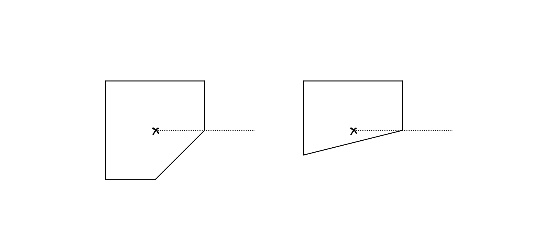
Figure 2. Drawn inside $B_{k}$ with the dashed ray representing the defining monodromy invariant ray. The left figure is the $k=1$, and the right one is $k=4$.

Recall that for $\mathcal{Y}$ a rigid analytic space a map $\mathcal{Y}\to B$ is continuous if the preimage of each admissible polygon is an admissible open of $\mathcal{Y}$ and the preimages of admissible coverings are admissible coverings in $\mathcal{Y}$. We call such a map strong Stein if the preimage of a admissible convex polygon is isomorphic to an affinoid domain as a rigid analytic space.

Proposition 3.14.

The map $p_{k}:Y_{k}^{an}\to B_{k}$ is a strongly Stein continuous map.

Proof.

For admissible polygons not containing the origin, the Stein property follows from Propositions 3.8 and 3.10. We also already know that the Stein property holds for $P(a)$ with $a>0$.

Assume that we already know the Stein property for an admissible polygon $P$ containing the node, i.e. that $p_{k}^{-1}(P)$ is an affinoid domain. Let $U$ be a rational halfspace containing the node in its interior. Now we claim that

$$p_{k}^{-1}(P\cap U)\subset p_{k}^{-1}(P)$$

is a Weierstrass subdomain (cf. [6, Proposition 3.3.2]). Consider the rational line $H$ that is the boundary of $U$ and use its $U$-co-orientation. Assume that $H$ is contained in $E^{+}(B^{+})$ (if it is contained in $E^{-}(B^{-})$ the same argument works). Then as in Equation (7) and using Proposition 3.8 we obtain a function $F\in\mathcal{O}(p_{k}^{-1}(Q))$ for any admissible polytope $Q\subset E^{+}(B^{+})$. Under the embedding $g^{+}$ the function $F$ is equal to $(\xi^{+})^{a}(\eta^{+})^{b}$ with $a\in\mathbb{Z}_{\geq 0}$ and $b\in\mathbb{Z}.$ Since $\xi$ and $(\eta^{+})^{\pm 1}$ are global functions, we obtain that $F$ in fact extends to functions in $\mathcal{O}(p_{k}^{-1}(Q))$ for any admissible polytope $Q\subset B_{k},$ particularly for $Q=P.$ To finish we notice that

$$p_{k}^{-1}(P\cap U)=\{x\in p_{k}^{-1}(P)\mid val(F(x))\geq b\}$$

for some $b\in\mathbb{R}$.

This finishes the proof of the Stein property since we can obtain each admissible polytope by successively chopping of some $P(a)$ by rational halfspaces. To finish it suffices to show that if $Q\subset P\subset B_{k}$ are admissible polygons such that $P$ contains the node but $Q$ does not, then $p_{k}^{-1}(Q)\subset p_{k}^{-1}(P)$ is an affinoid subdomain.

It suffices to deal with the case where $Q=P\cap U$ with $U$ a rational halfspace which does not contain the node. The same argument as above works, but this time we obtain

$$p_{k}^{-1}(P\cap U)=\{x\in p_{k}^{-1}(P)\mid val(F(x))\leq b\}$$

for some $F\in\mathcal{O}(p_{k}^{-1}(P))$. This means that we indeed have an affinoid subdomain, but this time a Laurent subdomain. ∎

Definition 3.15.

Let us define a sheaf $\mathcal{O}_{k}$ on the $G$-topology of $B_{k}$ by

$$\mathcal{O}_{k}(P):=\mathcal{O}(p_{k}^{-1}(P)),$$

for an admissible polygon $P$.

Corollary 3.16.

For $k\geq 0$, the sheaf $\mathcal{O}_{k}$ on the $G$-topology of $B_{k}$ satisfies the following properties

• (Affinoidness) If $P$ is an admissible convex polygon, $\mathcal{O}_{k}(P)$ is an affinoid algebra.

• (Subdomain) If $Q\subset P$ are admissible convex polygons, then the morphism of affinoid domains induced from the restriction map $\mathcal{O}_{k}(P)\to\mathcal{O}_{k}(Q)$:

  $$M(\mathcal{O}_{k}(P))\to M(\mathcal{O}_{k}(Q))$$

  has image an affinoid subdomain and it is an isomorphism of affinoid domains onto its image.

• (Strong cocycle condition) For admissible convex polygons $Q,Q^{\prime}\subset P$, we have

  $$im(M(\mathcal{O}_{k}(Q))\cap im(M(\mathcal{O}_{k}(Q^{\prime})))=im(M(\mathcal{O}_{k}(Q\cap Q^{\prime}))$$

  inside $M(\mathcal{O}_{k}(P))$

• (Independence) Let $Q_{1},\ldots,Q_{N}\subset P$ be admissible convex polygons such that $P=\bigcup Q_{i}$. Then

  $$\bigcup im(M(\mathcal{O}_{k}(Q_{i})))=M(\mathcal{O}_{k}(P)).$$

• (Separation) Let $Q\subset P$ be an inclusion of admissible convex polygons. For any $p\in M(\mathcal{O}_{k}(P))\setminus im(M(\mathcal{O}_{k}(Q))$ there is a small admissible polygon $Q^{\prime}\subset P$ which is disjoint of $Q$ such that $p\in im(M(\mathcal{O}_{k}(Q^{\prime})))$.

Proof.

We have already proved the first two properties in the proof of Proposition 3.14. The last three are also automatic because for $Q\subset P$ admissible polygons, we have

$$im(M(\mathcal{O}_{k}(Q))=p_{k}^{-1}(Q)\subset M(\mathcal{O}_{k}(P))$$

under the canonical identification of $M(\mathcal{O}_{k}(Q))$ with $p_{k}^{-1}(Q).$ ∎

We will also need the following Hartogs property.

Proposition 3.17.

Let $P\subset B_{k}$ be an admissible convex polygon containing the node. Then, restriction map

$$\mathcal{O}_{k}(P)\to\mathcal{O}_{k}(\partial P)$$

is an isomorphism.

Proof.

This follows from a much more general extension property in rigid analytic geometry, see [17, Proposition 2.5], and the proof of Proposition 3.14. Note that $Y_{k}^{an}$ is normal as analytification preserves normality [21, Proposition 1.3.5].

∎

Recall that in the previous section we defined on $Y_{0}$ (resp. $Y_{0}^{an}$) the algebraic (resp. analytic) volume form $\Omega_{0}$.

Proposition 3.18.

By taking the residue of the meromorphic form

$$Res_{Y_{k}\subset\mathbb{A}^{3}_{\Bbbk}}\left(-\frac{dxdydu}{u(xy-(u+1)^{k})}\right),$$

we can define an algebraic (resp. analytic) volume form $\Omega_{k}$ on the smooth points of $Y_{k}$ (resp. $Y_{k}^{an}$). The pullback of $\Omega_{k}$ under the embeddings $g^{\pm}$ is $\Omega_{0}$.

Proof.

Note that $\Omega_{k}$ is defined by the equality:

$$-\frac{dxdydu}{u(xy-(u+1)^{k})}=\frac{uydx+uxdy-(xy-(u+1)^{k-1})du}{u(xy-(u+1)^{k})}\wedge\Omega_{k}.$$

This implies the desired properties. For example when $x\neq 0$, we have $\Omega_{k}=\frac{dxdu}{xu}.$ ∎

4. Symplectic cohomology type invariants

4.1. Filtrations, torsion and boundary depth

A filtration map on an Abelian group $A$ is a map $\rho:A\to\mathbb{R}\cup\{\infty\}$ satisfying the inequality

$$\rho(x+y)\geq\min{(\rho(x),\rho(y))},$$

the equality $\rho(x)=\rho(-x)$, and sending $0$ to $\infty$. If $\rho^{-1}(\infty)=\{0\}$ the filtration map is called Hausdorff. A non-archimedean valuation on a $\Lambda$-vector space satisfies these assumptions along with multiplicativity for scalar multiplication.

Note that if $(V_{i},\rho_{i})$ are Abelian groups equipped with filtration maps indexed by a set $i\in I$, then $\bigoplus_{\alpha\in I}V_{\alpha}$ is equipped with a filtration map given by

$$\rho\left(\sum v_{i}\right):=\min_{i\in I}{\left(\rho_{i}(v_{i})\right)}.$$

Let us call this the $min$ construction.

Let us call an Abelian group with a filtration map a filtered Abelian group. Filtered Abelian groups are equipped with a pseudo-metric and topology. Let us call the value of an element under the filtration map the filtration value.

We call a graded Abelian group with a filtration map in each degree and a differential that does not decrease the filtration values a filtered chain complex. The homology of a filtered chain complex is naturally a filtered graded Abelian group by taking the supremum of the filtration values of all representatives for each homology class.

For $(C,d,\rho)$ a filtered chain complex and real numbers $a<b$, we define the subquotient complexes

$$C_{(a,b]}:=\frac{\{\rho>a\}}{\{\rho>b\}}.$$

Lemma 4.1.

Let $(C,d,\rho)$, $(C^{\prime},d^{\prime},\rho^{\prime})$ be filtered chain complexes whose underlying graded Abelian groups are degreewise Hausdorff and complete. Let $f:C\to C^{\prime}$ be a chain map which does not decrease the filtration values. Assume that for every $a<b$ real numbers, the induced map

$$C_{(a,b]}\to C^{\prime}_{(a,b]}$$

is a quasi-isomorphism, then $f$ is a quasi-isomorphism.

Proof.

This is an immediate consequence of the Eilenberg–Moore Comparison Theorem [29, Theorem 5.5.11]. ∎

If $A$ is a Novikov ring module, $A\otimes\Lambda$ is naturally equipped with a non-archimedean valuation as follows. Consider the natural map $\iota:A\to A\otimes\Lambda$. For $a\in A\otimes\Lambda$, we define

$$val_{A}(a):=-\inf\{r\in\mathbb{R}\mid T^{r}a\in\iota(A)\}.$$

Lemma 4.2.

If $A$ is a free Novikov ring module, then $val_{A}$ is a non-archimedean valuation on $A\otimes\Lambda$. We can complete $A$ as a Novikov ring module $\hat{A}$ and complete $A\otimes\Lambda$ as a normed space $\widehat{A\otimes\Lambda}$. Then, the natural map

$$\hat{A}\otimes\Lambda\to\widehat{A\otimes\Lambda}$$

is a valuation preserving functorial isomorphism.

Definition 4.3.

Let $A$ be a module over the Novikov ring $\Lambda_{\geq 0}$. For any element $v\in A$ we define the torsion $\tau(v)$ to be the infimum over $\lambda$ so that $T^{\lambda}v=0$. We take $\tau(v)=\infty$ if $v$ is non-torsion. We define the maximal torsion

(32) $$\tau(A):=\sup_{v:\tau(v)<\infty}\tau(v).$$

If there are no torsion elements we take $\tau(A)=-\infty$.

Lemma 4.4.

The natural map $\iota:A\to A\otimes\Lambda$ is injective if and only if $A$ has no torsion elements.

The importance of the following definition was explained thoroughly in [9].

Definition 4.5.

For any $C$ chain complex over $\Lambda_{\geq 0}$, we define the $i$- homological torsion of $C$ as the maximal torsion of $H^{i}(C)$. If the $i$-homological torsion of $C$ is less than $\infty$, we say that it has homologically finite torsion at degree $i$.

Now we relate it to the notion of finite boundary depth which to the best of our knowledge was introduced to symplectic topology by Usher [26].

Definition 4.6.

Let $(C,d,\rho)$ be a Hausdorff filtered chain complex. The boundary depth in degree $i\in\mathbb{Z}$ is defined as the infimum of $\beta\geq 0$ satisfying

$$\text{ for every }x\in im(d)\cap C^{i},\text{there exists y}\in C^{i-1}\text{ s. t. }dy=x\text{ and }\rho(x)-\rho(y)\leq\beta.$$

If this is not $+\infty$ we say that the boundary depth is finite in degree $i$. If the boundary depth is finite in all degrees we say that $C$ has finite boundary depth.

Proposition 4.7.

Assume that $(C,d,\rho)$ is obtained from a chain complex over the Novikov ring $C^{\prime}$ i.e. $C=C^{\prime}\otimes_{\Lambda_{\geq 0}}\Lambda$, where the underlying module of $C^{\prime}$ is torsion free. Then the boundary depth in degree $i$ is equal to the maximal torsion of $H^{i}(C^{\prime})$.

Proof.

For an element $\alpha\in C$ and $\delta>0$, there is a unique element $\alpha_{0,\delta}\in C^{\prime}$ such that

$$\alpha=T^{\rho(\alpha)-\delta}\alpha_{\delta}\otimes 1.$$

Let us first show that $b_{i}$, the boundary depth in degree $i$, is at least $t_{i}$, the maximal torsion in degree $i$. Let $[z]\in H^{i}(C^{\prime})$ be an arbitrary torsion element. Then, it follows that $z\otimes 1\in C^{i}$ is exact. For every $\epsilon>0$, there exists

$$y\in C^{i-1}\text{ s. t. }dy=z\otimes 1\text{ and }-\rho(y)\leq b_{i}+\epsilon-\rho(z\otimes 1)\leq b_{i}+\epsilon.$$

Since $d$ does not decrease $\rho$ values, $T^{-\rho(y)+\epsilon}z$ defines an element in $C^{\prime}$. It immediately follows that $T^{-\rho(y)+\epsilon}z=dy_{\epsilon}$ and that $T^{b_{i}+2\epsilon}[z]=0$. We proved that $b_{i}+2\epsilon\geq t_{i}$, which implies the claim.

Conversely, let us consider an exact element $x\in C^{i}$. Then, it follows that $x_{\delta}$ is torsion for all $\delta>0$. Therefore, there exists $y_{\delta}$ such that $dy_{\delta}=T^{t_{i}+\delta}x_{\delta}$. But, then

$$T^{\rho(x)-t_{i}-2\delta}d(y_{\delta}\otimes 1)=T^{\rho(x)-2\delta-t_{i}}T^{t_{i}+\delta}x_{\delta}\otimes 1=x.$$

Note that

$$\rho(x)-\rho(T^{\rho(x)-t_{i}-2\delta}y_{\delta}\otimes 1)\leq t_{i}+2\delta$$

This shows that $b_{i}\leq t_{i}+2\delta$, finishing the proof.

∎

Corollary 4.8.

Using the notation and assumptions of Proposition 4.7, the complex $C$ has finite boundary depth in degree $i$ if and only if the complex $C^{\prime}$ has homologically finite torsion in degree $i$.

We will also need the following lemma.

Lemma 4.9.

Let $X$ be a Hausdorff filtered abelian group and $Y$ a subspace. Then the completion of $X/Y$ is isomorphic to $\widehat{X}/\bar{Y},$ where $\bar{Y}$ is the closure of $Y\subset\widehat{X}$.

Proof.

First, note that $\widehat{X}/\bar{Y}$ is complete. We also have a canonical map

$$q:X/Y\to\widehat{X}/\bar{Y},$$

because $X\to\widehat{X}\to\widehat{X}/\bar{Y}$ factors through $X/Y$. We claim that $q$ satisfies the universal mapping property of the completion of $X/Y$ in the category of filtered abelian groups with bounded linear maps, which finishes the proof.

Let $X/Y\to Z$ be any map in this category with $Z$ complete. By pre-composing with the quotient map we obtain a map $X\to Z$, which factors through $X\to\widehat{X}$ to give $\widehat{X}\to Z$ by the UMP of completion. This last map sends $Y$ to zero, which implies that it sends $\bar{Y}$ to zero by continuity. Therefore, we get the desired factorization through $q$. The uniqueness also follows because otherwise we contradict the uniqueness part of the UMP for $X\to\widehat{X}$ noting that $\widehat{X}\to\widehat{X}/\bar{Y}$ is surjective. ∎

4.2. Relative symplectic cohomology

Let $M$ be a geometrically bounded symplectic manifold and $K$ a compact subset. Let us also fix a homotopy class of trivializations of the canonical bundle $K_{M}$. Then we obtain a unital $\mathbb{Z}$-graded BV algebra over the Novikov field

$$SH^{*}_{M}(K,\Lambda):=SH^{*}_{M}(K)\otimes\Lambda.$$

From now on we will only consider unital and ${\mathbb{Z}}$-graded BV algebras, and we will omit mentioning this. The construction of $SH^{*}_{M}(K,\Lambda)$ involves the choice of a monotone acceleration datum and various other choices of monotone Floer data to construct the BV operator and the pair-of-pants product. The unit was constructed in [25]. One can show of such data different choices give rise to canonically isomorphic BV algebras. For more details see [9, Section 6.2] . Note that using

(33) $$\mathcal{C}:=CF^{*}(H_{1};\Lambda_{\geq 0})\to CF^{*}(H_{2};\Lambda_{\geq 0})\ldots$$

as the defining Floer one ray, we can equip $tel(\mathcal{C})\otimes\Lambda$ with its natural filtration map. We then have by Lemma 4.2 that

$$H^{*}(\widehat{tel(\mathcal{C})\otimes\Lambda})$$

is canonically isomorphic as filtered BV algebras with $SH^{*}_{M}(K,\Lambda)$.

We can also define an invariant for open sets. Let $U$ be an open subset of $M$. Let $K_{1}\subset K_{2}\subset\ldots$ be an exhaustion of $U$ by compact subsets. We define

$$SH^{*}_{M}(U,\Lambda):=\varprojlim SH^{*}_{M}(K_{i},\Lambda).$$

Remark 4.10.

In the present work we will only consider the case $U=M$. In the case considered here, $SH^{0}_{M}(M)$ will be the entire functions of the mirror.

Lemma 4.11.

It is easy to see by functoriality of $SH^{*}_{M}(\cdot)$ with respect to inclusions that $SH^{*}_{M}(U)$ is independent of the choice of exhaustion in the sense that different exhaustions of $U$ give rise to canonically isomorphic $SH^{*}_{M}(U).$

4.3. Exact manifolds

Let $(M,\theta)$ be an exact graded symplectic manifold that is of geometrically finite type and assume that $W\subset M$ is a compact domain. Then we can work over the base commutative ring $\mathbb{F}$ (coefficient ring for the elements of $\Lambda$), e.g. $\mathbb{F}=\mathbb{Z}$. We consider $\mathbb{F}$ as a trivially valued field.

We choose a dissipative acceleration datum for $W$ whose underlying Hamiltonians $H_{i}$ each have finitely many $1$-periodic orbits. Define a Floer $1$-ray over $\mathbb{F}$ by signed counts without weights:

$$\mathcal{C}_{\mathbb{F}}:=CF^{*}(H_{1};\mathbb{F})\to CF^{*}(H_{2};\mathbb{F})\ldots$$

and obtain

$$SH^{*}_{M,\theta}(W;\mathbb{F}):=H^{*}(\widehat{tel}(\mathcal{C})),$$

which is a BV algebra over $\mathbb{F}$. Here the filtration map on the telescope comes from taking the actions of generators

$$A(\gamma)=\int\gamma^{*}\theta+\int H(\gamma(t))dt,$$

and equipping the telescope with the min-filtration (by taking the minimum of the filtration values of the basis elements in the linear combination). We obtain a filtration map on $SH^{*}_{M,\theta}(W;\mathbb{F})$ by taking supremum of chain representatives. The operations do not decrease the filtration map in the appropriate sense.

Theorem 4.12.

$SH^{*}_{M,\theta}(W;\mathbb{F})$ is well-defined as a filtered graded Abelian group, i.e. another choice of dissipative acceleration data gives rise to a filtered graded Abelian group which is canonically isomorphic in a way that preserves filtration maps.

Proof.

This follows from combining [8, Lemma 8.14] and Lemma 4.1 ∎

Remark 4.13.

This statement would not be true if we did not complete the telescope. This can be seen by comparing $S$-shaped and $J$-shaped acceleration data for Liouville manifolds.

In many situations relevant to this paper (see Proposition 5.3), we observe that the acceleration data can be chosen to satisfy the extra property that the actions of the $1$-periodic orbits that contribute are uniformly bounded above (e.g. non-positive). The completion to the telescope of $\mathcal{C}_{\mathbb{F}}$ does nothing in this case! Let us call this the bounded action property.

Lemma 4.14.

Under the bounded action property, the induced pseudo metric on $SH^{*}_{M,\theta}(W;\mathbb{F})$ is actually a metric and the topology is complete and Hausdorff.

Here is the main application of boundary depth considerations for our purposes.

Proposition 4.15.

Let us assume that $tel(\mathcal{C}_{\mathbb{F}})$ has finite boundary depth at degree $i$. Then, the canonical map

$$SH^{i}_{M,\theta}(W;\mathbb{F})\hat{\otimes}\Lambda\to SH_{M}^{i}(W;\Lambda)$$

obtained by action rescaling is a filtered isomorphism.

Proof.

Define $\mathcal{C}:=CF^{*}(H_{1};\Lambda_{\geq 0})\to CF^{*}(H_{2};\Lambda_{\geq 0})\ldots$ as in Equation (33). We have a filtered isomorphism of chain complexes

$$tel(\mathcal{C}_{\mathbb{F}})\otimes\Lambda\to tel(\mathcal{C})\otimes_{\Lambda_{\geq 0}}\Lambda,$$

given by sending

$$\gamma\otimes 1\mapsto\gamma\otimes T^{A(\gamma)}.$$

Let us define $(C^{*},d^{*})$ to be the normed $\Lambda$-chain complex $\widehat{tel}(\mathcal{C}_{\mathbb{F}})\otimes\Lambda$ and $(\widehat{C}^{*},\widehat{d}^{*})$ be the degree-wise completion. We can write any homogeneous element $x\in\widehat{C}^{i}$ as an infinite sum $\sum_{n=0}^{\infty}\alpha_{n}\otimes T^{a_{n}}$ with $\alpha_{n}\in\widehat{tel}(\mathcal{C}_{\mathbb{F}})^{i}$ and $a_{n}\in\mathbb{R}$ pairwise distinct such that $A(\alpha_{n})+a_{n}\to\infty$. The valuation of such an element is the minimum of $A(\alpha_{n})+a_{n}$.

We have that $SH_{M}^{i}(W;\Lambda)$ is isomorphic to

$$ker(\widehat{d}_{i})/im(\widehat{d}_{i-1}),$$

and $SH^{i}_{M,\theta}(W;\mathbb{F})\hat{\otimes}\Lambda$ is nothing but

$$\widehat{ker(d_{i})/im(d_{i-1})}.$$

Our goal is to use Lemma 4.9 to finish the proof.

Note that $ker(\widehat{d}_{i})$ and $\widehat{ker(d_{i})}$ are both canonically identified with the subset of $\widehat{C}^{i}$ consisting of elements $\sum_{n=0}^{\infty}\alpha_{n}\otimes T^{a_{n}}$ with $\alpha_{n}$ closed in $\widehat{tel}(\mathcal{C}_{\mathbb{F}})^{i}$. Hence all that is left to show is that $im(\widehat{d}_{i-1})$ is the closure of $im({d}_{i-1})$ inside $\widehat{C}^{i}$ (and hence inside $\widehat{ker(d_{i})}$).

Continuity immediately implies that $im(\widehat{d}_{i-1})$ is in the closure. Conversely, we can write every limit point as $\sum_{n=0}^{\infty}\alpha_{n}\otimes T^{a_{n}}$ with each $\alpha_{n}$ exact. The finite boundary depth assumption finishes the proof as it lets us construct a primitive with respect to $\widehat{d}_{i}$. ∎

4.4. Liouville manifolds

We now discuss the relation between relative $SH$ and the symplectic cohomology introduced by Viterbo mainly for Liouville domains and their completions. Here we refer in particular to the non-quantitative approach emphasised in Section 3e) of [22].

Let $(M,\theta)$ be a finite type complete Liouville manifold and denote by $Z$ the Liouville vector field. Let $W\subset M$ be a compact domain with smooth boundary such that the Liouville vector field $V$ is outward pointing on $\partial W$ and $V$ is non-zero outside of $W$. Call such a domain admissible. Denoting by $Sk_{\theta}$ the skeleton of $M$ with respect to $\theta$, $\partial W$ and $V$ give rise to an exponentiated Liouville coordinate

$$\rho:M\setminus Sk_{\theta}\to\mathbb{R}_{>0},$$

which is equal to $1$ on $\partial W$ and satisfies $V\cdot\rho=\rho.$ Let us denote by $\mathcal{L}(W)$ the class of Hamiltonians on $M$ which outside of a compact set are linear functions of $\rho$. Define a pre-order on $\mathcal{L}(W)$ by $H_{i}\preceq H_{i+1}$ if there is a constant $C$ for which $H_{1}\leq H_{2}+C$.

We then get an invariant $SH^{*}(M;\mathbb{F})$ which we refer to as Viterbo $SH$. It is defined by considering the non-completed colimit of the Floer complexes for any sequence of Hamiltonians $H_{i}\in\mathcal{L}(W)$ with the slope going to infinity. Since the sequence $H_{i}$ is only required to satisfy that $H_{i+1}-H_{i}$ is bounded from below, the Viterbo $SH$ contains no quantitative information about the domain $W$.

At first sight there is still some dependence on the domain $W$ because of the involvement of $\mathcal{L}(W)$. However, as pointed out in [22], the Viterbo symplectic cohomologies for different admissible subdomains $W$ are canonically isomorphic. The reason is that we can squeeze a sequence in $\mathcal{L}(W_{1})$ into any sequence in $\mathcal{L}(W_{2})$ and vice versa. Moreover, given functions $H_{1},H_{2}$ which at infinity are linear functions of $\rho_{1},\rho_{2}$ respectively, and satisfying $H_{1}\leq H_{2}+C$ there are well defined continuation maps between them .

It is convenient to push this discussion somewhat further. Denote by $\mathcal{L}_{a}(W)$ the set of dissipative functions $H$ on $M$ for which there exists a $c$ so that $\frac{1}{c}\rho<H<c\rho$ outside of a compact set. Since for $W_{1},W_{2}$ we have constants $\frac{1}{c}\rho_{1}<\rho_{2}<c\rho_{1}$ there is actually an equality $\mathcal{L}_{a}(W_{1})=\mathcal{L}_{a}(W_{2})$. We thus drop the dependence on $W$ from the notation and write $\mathcal{L}=\mathcal{L}_{a}(W)$.

Then $\mathcal{L}(W)\subset\mathcal{L}$ is $\preceq$-cofinal. It follows that the Viterbo $SH$ can be computed with any $\preceq$-cofinal sequence in $\mathcal{L}$.

Remark 4.16.

The Viterbo $SH$ is a global invariant of $M$, but it is not naturally endowed with a norm. The interpretation of Viterbo $SH$ for exact symplectic cluster manifolds is as the functions of the algebraic mirror defined over $\mathbb{F}$.

As observed in [8] Viterbo $SH$ can also be defined for $M$ which is not necessarily the completion of a Liouville domain (not even exact) provided one specifies an appropriate growth condition at infinity akin to the set $\mathcal{L}$. In the case we are considering, the integral affine structure can be used to specify such a condition, namely, piece-wise linearity in integral affine coordinates. In particular this specifies a set of global algebraic functions on the mirror over the Novikov field.

We now compare Viterbo $SH$ to relative $SH$ of a compact domain $W\subset M$. We drop the requirement that $W$ has smooth boundary. We only require that $W$ is the intersection of a descending sequence of admissible subdomains $W_{i}$. Then in computing relative $SH$ of $W$ we can use acceleration data of Viterbo type. Namely, if $W=\cap_{i=1}^{\infty}W_{i}$ the underlying $i$th Hamiltonian is a linear function of $\rho_{i}$ near infinity, a convex function of $\rho_{i}$ on $M\setminus W_{i}$ and $C_{2}$ small on $W_{i}$. For such acceleration data one can immediately see from the Viterbo $y$-intercept trick that the action functional really only takes negative values. This means that the filtration map can only take non-positive values. Note that the sequence of Hamiltonians of this acceleration datum is $\preceq$ cofinal in $\mathcal{L}$. We thus conclude

Theorem 4.17.

1. $SH^{*}_{M,\theta}(W;\mathbb{F})$ is canonically isomorphic to the Viterbo symplectic cohomology $SH^{*}(M;\mathbb{F})$ of $M$ as a BV-algebra

2. If $W^{\prime}\subset M$ also satisfies the conditions above, $SH^{*}_{M,\theta}(W;\mathbb{F})$ and $SH^{*}_{M,\theta}(W^{\prime};\mathbb{F})$ are canonically isomorphic BV algebras.

Remark 4.18.

These isomorphisms are a special feature of the exact case and even then only hold over a trivially valued field. For example the isomorphism in the second part does not have to be bounded with respect to the filtration. Thus if we base change to a non-trivially valued field the completions will be different and the canonical restriction map will no longer be an isomorphism. For example consider $M=T^{*}S^{1}\cong\mathbb{R}\times S^{1}$, $W=[-1,1]\times S^{1}$ and $W^{\prime}=[-2,2]\times S^{1}.$ Identifying the algebra with Laurent series in the variable $z$ the infinite series $\sum T^{-i}z^{i}$converges with respect to the first norm, but not the second.

There are many techniques to compute the Viterbo symplectic cohomology as a BV algebra. Most important among them is Viterbo’s isomorphism between symplectic cohomology and string homology in case of the cotangent bundle of a smooth manifold. The latter is fully computable for $T^{n}$, which we will use below (see Theorem 5.1). On the other hand what is relevant for us is the completed version (assuming finite boundary depth as above)

$$SH^{*}_{M,\theta}(W;\mathbb{F})\hat{\otimes}\Lambda=SH_{M}^{*}(W;\Lambda)$$

as we are planning to use our locality theorem in more global situations. Hence, it is important to be able to explicitly describe the norm on $SH^{*}(M;\mathbb{F})$ given by $W$ as above.

5. Analysis of the local model for the regular fibers

We denote the coordinate functions of ${\mathbb{R}}^{n}$ by $q_{1},\ldots q_{n}$ and the corresponding dual linear coordinates on $({\mathbb{R}}^{n})^{\vee}$ by $p_{1},\ldots p_{n}$. $\mathbb{Z}^{n}$ and $(\mathbb{Z}^{n})^{\vee}$ are the standard integer lattices in $\mathbb{R}^{n}$ and $(\mathbb{R}^{n})^{\vee}.$ Let us denote the smooth manifold underlying ${\mathbb{R}}^{n}$ by $B_{0}$ for clarity. Let $v$ be the vector field $\sum q_{i}\frac{\partial}{\partial q_{i}}$ in $B_{0}$. Note that this vector field is invariant under the action of linear isomorphisms of ${\mathbb{R}}^{n}$.

Let $M:=({\mathbb{R}}^{n})^{\vee}/(\mathbb{Z}^{n})^{\vee}\times{\mathbb{R}}^{n}$ be equipped with the Liouville structure $\theta:=\sum-q_{i}dp_{i}$ and let $\omega:=d\theta$. Let $\pi:M\to B_{0}$ be the canonical projection and equip $\pi$ with the induced (trivial) horizontal subbundle. The horizontal lift $V$ of $v$ is the Liouville vector field.

Let us also trivialize the canonical bundle $TM_{\mathbb{C}}^{\wedge n}$ defined through the compatible almost complex structure $J\frac{\partial}{\partial q_{i}}=-\frac{\partial}{\partial p_{i}}$ with the trivialization

$$\frac{\partial}{\partial q_{1}}\wedge\ldots\wedge\frac{\partial}{\partial q_{n}}.$$

We will now state a special case of Viterbo’s theorem, Theorem 1.1 of [15, Chapter 12]. Note that $M$ is symplectomorphic to the cotangent bundle of $T^{n}$

$$\left(T^{*}(({\mathbb{R}}^{n})^{\vee}/(\mathbb{Z}^{n})^{\vee})=({\mathbb{R}}^{n})^{\vee}/(\mathbb{Z}^{n})^{\vee}\times{\mathbb{R}}^{n},\sum dp_{i}dq_{i}=-\omega\right)$$

via the map that negates the $q$ coordinates. Using the computation of the Chas-Sullivan string homology BV-algebra from [24, Section 6.2], we know that the symplectic cohomology of $T^{*}T^{n}$ is isomorphic to

$$\mathbb{F}[H_{1}(T^{n},\mathbb{Z})]\otimes\Lambda^{*}(H^{1}(T^{n},\mathbb{Z}))$$

with the $BV$ operator given by taking the interior product of an element of $\Lambda^{*}(H^{1}(T^{n},\mathbb{Z}))$ with an element of $H_{1}(T^{n},\mathbb{Z}).$

Theorem 5.1.

The Viterbo symplectic cohomology $BV$-algebra $SH^{*}(M;\mathbb{F})$ is isomorphic to

$$\mathcal{A}^{*}:=\mathbb{F}[(\mathbb{Z}^{n})^{\vee}]\otimes\Lambda^{*}(\mathbb{Z}^{n}),$$

with its implicit graded algebra structure and the $BV$ operator:

$$\Delta(z^{\alpha}\otimes\beta)=z^{\alpha}\otimes\iota_{\alpha}\beta,$$

for any $\alpha\in(\mathbb{Z}^{n})^{\vee}$ and $\beta\in\Lambda^{*}(\mathbb{Z}^{n})$.

Moreover, using the identification $H_{1}(M;\mathbb{Z})=(\mathbb{Z}^{n})^{\vee}$, and the extra $H_{1}(M;\mathbb{Z})$-grading of $SH^{*}(M;\mathbb{F})$ obtained using the homology classes of orbits

• the homogeneous summand of $SH^{0}(M;\mathbb{F})$ corresponding to the homology class $\alpha\in(\mathbb{Z}^{n})^{\vee}$ is generated by $z^{\alpha}\otimes 1$ as an $\mathbb{F}$-module.

• the homogeneous summand $SH^{*}_{0}(M;\mathbb{F})$ of $SH^{*}(M;\mathbb{F})$ corresponding to the homology class $0\in(\mathbb{Z}^{n})^{\vee}$ is generated by $1\otimes e_{i},i=1,\ldots,n$ as an $\mathbb{F}$-algebra.

• The homogeneous summand of $SH^{*}(M;\mathbb{F})$ corresponding to the homology class $\alpha\in(\mathbb{Z}^{n})^{\vee}$ is generated by $z^{\alpha}\otimes 1$ as an $SH^{*}_{0}(M;\mathbb{F})$-module

Recall that at the end of Section 3.1, for an admissible convex polytope $P\subset B_{0}$, we defined the $BV$-algebra $\mathcal{A}^{*}(P)$.

Proposition 5.2.

The natural map of $\Lambda$-algebras

$$\mathcal{A}^{*}\otimes\Lambda\to\mathcal{A}^{*}(P)$$

given by

$$z^{e_{i}^{\vee}}\otimes 1\otimes 1\to y_{i}^{-1}\text{ and }1\otimes e_{j}\otimes 1\to y_{j}\frac{\partial}{\partial y_{j}}$$

respects the BV operator. Moreover, it is injective and has dense image.

Proof.

We need to check what happens to

(34) $$z^{\alpha}\otimes e_{j(1)}\wedge\ldots\wedge\ldots e_{j(k)}\otimes 1,$$

for $\alpha\in(\mathbb{Z}^{n})^{\vee}$ and $j:[k]\to[n]$ strictly order preserving. It’s image under BV operator is

$$z^{\alpha}\otimes\sum_{l=1}^{k}(-1)^{l-1}\alpha(e_{j(l)})\cdot e_{j(1)}\wedge\ldots\widehat{e_{j(l)}}\wedge\ldots e_{j(k)}\otimes 1.$$

Applying the natural map in turn, we get

$$y^{-\alpha}\sum_{l=1}^{k}(-1)^{l+1}\alpha(e_{j(l)})\cdot y^{e_{j(1)}^{\vee}+\ldots+\widehat{e_{j(l)}^{\vee}}+\ldots+e_{j(k)}^{\vee}}\frac{\partial}{\partial y_{j(1)}}\ldots\widehat{\frac{\partial}{\partial y_{j(l)}}}\ldots\frac{\partial}{\partial y_{j(k)}},$$

Under the natural map (34) is sent to

$$y^{-\alpha+e_{j(1)}^{\vee}+\ldots+e_{j(k)}^{\vee}}\frac{\partial}{\partial y_{j(1)}}\ldots\frac{\partial}{\partial y_{j(k)}}.$$

The inner product with $\Omega_{0}$ returns

$$(-1)^{s(j)}y^{-\alpha-e_{j^{\prime}(1)}^{\vee}-\ldots-e_{j^{\prime}(n-k)}^{\vee}}dy_{j^{\prime}(1)}\ldots dy_{j^{\prime}(n-k)},$$

where

$$s(j):=\sum_{l=1}^{k}j(l)-l,$$

and $j^{\prime}:[n-k]\to[n]$ is the order preserving isomorphism to the complement of the image of $j$.

Exterior differential of this is

$$(-1)^{s(j)}y^{-\alpha-e_{j^{\prime}(1)}^{\vee}-\ldots-e_{j^{\prime}(n-k)}^{\vee}}\sum_{l=1}^{k}(-1)^{j(l)-l}(-\alpha(e_{j(l)}))\cdot y^{-e_{j(l)}^{\vee}}dy_{j^{\prime}(1)}\ldots dy_{j(l)}\ldots dy_{j^{\prime}(n-k)}.$$

This then goes back to

$$\sum_{l=1}^{k}(-1)^{s(j)+s(j\setminus l)+j(l)+l+1}y^{-\alpha+e_{j(1)}^{\vee}+\ldots+\widehat{e_{j(l)}^{\vee}}+\ldots+e_{j(k)}^{\vee}}\alpha(e_{j(l)})\cdot\frac{\partial}{\partial y_{j(1)}}\ldots\widehat{\frac{\partial}{\partial y_{j(l)}}}\ldots\frac{\partial}{\partial y_{j(k)}},$$

where $j\setminus l$ denotes the map $[k-1]\to[k]\to[n]$ with the first map isomorphism on to the complement of $\{l\}$.

It is easy to see that

$$s(j)-s(j\setminus l)=j(l)-l+(k-l).$$

Applying the final sign $(-1)^{k}$ we obtain the correct result. ∎

Let us recall some generalities on integrable Hamiltonian flows on $M$. Note that the vertical tangent space of $\pi$ at any $x\in M$, is canonically identified with $T^{*}_{\pi(x)}B_{0}=(\mathbb{R}^{n})^{\vee}$. The Hamiltonian vector field of any $H=h\circ\pi$ at $x$ (which is vertical) is equal to $dh_{\pi(x)}$ under this identification. Hence the Hamiltonian flow of such an $H$ preserves the fibers of $\pi$, and inside each torus the time $t$ map of the flow is given by translating the torus $\pi^{-1}(b)=(\mathbb{R}^{n})^{\vee}/(\mathbb{Z}^{n})^{\vee}$ by the vector $tdh_{\pi_{b}}.$ In particular, the time $1$ periodic orbits of the Hamiltonian flow of $H$ correspond to the $b\in B_{0}$ such that $dh_{b}$ is integral.

Let us denote the Hamiltonian flow of $H=h\circ\pi$ by $\Phi^{t}$. The flow $\Phi^{t}$ does not preserve the horizontal subspaces. The image of a horizontal vector $v\in H_{x}\subset T_{x}M$ under $d\Phi^{t}$ is given by the sum of the horizontal lift of $\pi_{*}v$ to $\Phi_{t}(x)$ and the vertical vector corresponding to

$$t\nabla_{\pi_{*}v}dh\in T_{\pi(x)}^{*}B,$$

where the bilinear form $\nabla dh$ on $T_{b}B$ has matrix

$$\left(\frac{\partial^{2}h}{\partial q_{i}\partial q_{j}}(b)\right)$$

with respect to basis $\frac{\partial}{\partial q_{1}},\ldots,\frac{\partial}{\partial q_{n}}.$

Hence the Morse-Bott non-degeneracy of a time-$1$ orbit of $\Phi^{t}$ corresponding to a point $b\in B$ with integral $dh_{b}$ is equivalent to the non-degeneracy of the symmetric bilinear form $(\nabla dh)_{b}$. The Maslov index [20] of this path is equal to $-s/2$, where $s$ is the the number of positive eigenvalues minus the number of negative eigenvalues of $(\nabla dh)_{b}$ using the Normalization property listed in page 17 of [20]. Our convention is to add $n$ to the Maslov index to define the degree in our Floer complexes. After controlled perturbations to $H$, such a $b$ therefore contributes $H^{*+n-s/2}(T^{n};\mathbb{Z})$ to the Hamiltonian Floer cohomology.

The following generalization of Viterbo’s $y$-intercept formula for actions will be useful. We state it more generally than needed here using the same notation.

Proposition 5.3.

Let $M$ be an exact symplectic manifold and $\rho:M\to\mathbb{R}^{k}$ be an involutive smooth map. Assume that the Liouville vector field $V$ on $M$ and the Euler vector field $v$ in the base $\mathbb{R}^{k}$ are $\rho$-related. Let $h:\mathbb{R}^{k}\to\mathbb{R}$ be smooth and $H:=h\circ\rho$. Then the action of a $1$-periodic orbit $\gamma:S^{1}\to M_{k}$ of $H$ living over $b\in\mathbb{R}^{k}$ is

$$\int\gamma^{*}\theta+\int\gamma^{*}H=h(b)+\int_{0}^{1}\theta(X_{H}(\gamma(t))dt.$$

Using

$$\theta(X_{H})=\omega(Z,X_{H})=-dH(Z)=-dh(V),$$

we obtain precisely that the action is given by the height axis intercept of the tangent space to the graph of $h$ over $b$.

For $\alpha\in(\mathbb{Z}^{n})^{\vee}$ and $Q\subset B_{0}^{n},$ we define $F(Q,\alpha)$ to be the subset of $Q$ where $\alpha:B_{0}^{n}={\mathbb{R}}^{n}\to\mathbb{R}$ takes its maximum on $Q$.

Proposition 5.4.

Let $P\subset B_{0}^{n}$ be an admissible convex polytope containing the origin. Then,

1. There exists an acceleration datum for $\pi^{-1}(P)\subset M$ leading to the Floer $1$-ray $\mathcal{C}_{\mathbb{F}}:=CF^{*}(H_{1};\mathbb{F})\to CF^{*}(H_{2};\mathbb{F})\ldots$ such that the bounded action property is satisfied and $tel(\mathcal{C}_{\mathbb{F}})$ has finite boundary depth at all degrees.

2. The map obtained by Theorem 4.17 and Theorem 5.1

   $$SH^{*}_{M,\theta}(\pi^{-1}(P),\mathbb{F})\to\mathbb{F}[(\mathbb{Z}^{n})^{\vee}]\otimes\Lambda^{*}(\mathbb{Z}^{n})$$

   is so that the induced filtration map (via Theorem 4.12) on $\mathbb{F}[(\mathbb{Z}^{n})^{\vee}]\otimes\Lambda^{*}(\mathbb{Z}^{n})$ is

   $$\sum a_{i}z^{\alpha_{i}}\otimes\beta_{i}\mapsto\min_{i}-\alpha_{i}(F(P,\alpha_{i}))=\min_{i}\min_{b\in P}-\alpha_{i}(b).$$

Proof.

Assume that $P$ can be defined by the inequalities:

$$\nu_{i}(p)\geq b_{i},$$

where $\nu_{i}$ are primitive elements of $(\mathbb{Z}^{n})^{\vee}$ and $b_{i}\in\mathbb{R}$ for $i=1,\ldots k$.

Let us define for $\eta>0$ the functions

$$l_{i,\eta}(x)=b_{i}-\eta-\nu_{i}(x),$$

for $x\in B_{0}^{n}$. For any $\vec{\lambda}\in\mathbb{R}_{>0}^{k},$ we define

$$h_{\vec{\lambda},\eta}:=\max{(0,\lambda_{1}l_{1,\eta},\ldots,\lambda_{k}l_{k,\eta})}$$

and also $\nu_{\vec{\lambda}}^{-}$ be an arbitrary function $\mathbb{R}^{n}\to(\mathbb{R}^{n})^{\vee}$ equal to $dh_{\vec{\lambda}}$ whenever the latter makes sense.

Let $\rho_{\epsilon}:\mathbb{R}^{n}\to\mathbb{R}$, $\epsilon\geq 0$ be a choice of mollifiers which approximate the Dirac delta function. We will only consider $\epsilon$’s small which are sufficiently small.

We also consider a parameter $\delta\geq 0$ and define

$$h_{\vec{\lambda},\eta,\epsilon,\delta}:=\rho_{\epsilon}\star h_{\vec{\lambda},\eta}-\delta.$$

Let us also define $h_{\vec{\lambda},\epsilon}:=h_{\vec{\lambda},\epsilon,0}.$ Note that we have that

$$(dh_{\vec{\lambda},\eta,\epsilon,\delta})_{b}=\int_{\mathbb{R}^{n}}\rho_{\epsilon}(b-y)\nu_{\vec{\lambda}}^{-}(y)dy.$$

Let us call $\vec{\lambda}\in\mathbb{R}_{>0}^{k}$ sufficiently irrational, if the boundary of the intersection complex of the points

$$\lambda_{1}\nu_{1},\ldots,\lambda_{k}\nu_{k}\in(\mathbb{R}^{n})^{\vee}$$

does not contain any integral points. Here by intersection complex we mean the union of

$$\left\{\sum_{i\in S}a_{i}\lambda_{i}\nu_{i}\mid\sum_{i\in S}a_{i}\leq 1,a_{i}\geq 0\right\}$$

over all non-empty subsets $S$ of $[k]$ such that the faces of $P$ associated to $\nu_{i}$ with $i\in S$ have non-empty intersection. Let us call this convex polytope $I_{\vec{\lambda}}$.

If $\vec{\lambda}$ is sufficiently irrational (which we assume from now on) then $h_{\vec{\lambda},\epsilon,\delta}$ is dissipative with respect to the standard $J$ coming from the flat metric on $\mathbb{R}^{n}$. Indeed the Hamiltonians are Lipschitz with respect to this $J$ and we have a uniform bound from below outside of the pre-image of the complement of a neighborhood of $P$ on the distance of a point to its time $1$ flow. The dissipativity then follows by Lemma 5.11 and Corollary 6.19 of [8].

All functions $h_{\vec{\lambda},\epsilon,\delta}$ are convex. We can consider the map

$$\mathbb{R}^{n}\to(\mathbb{R}^{n})^{\vee}$$

which sends

$$b\mapsto(-dh_{\vec{\lambda},\epsilon,\delta})_{b}.$$

The image is $I_{\vec{\lambda}}$ and we can almost explicitly compute the preimage $X_{\alpha}$ of each $\alpha\in(\mathbb{Z}^{n})^{\vee}\cap I_{\vec{\lambda}}$. $X_{\alpha}$ is an admissible polytope with the same dimension as $F(P,\alpha)$. It is also parallel to $F(P,\alpha)$ and converges to $F(P,\alpha)$ as $\epsilon\to 0$.

We can perturb $h_{\vec{\lambda},\epsilon,\delta}$ to $\tilde{h}_{\vec{\lambda},\epsilon,\delta}$ by a $C_{2}$ small function supported in an arbitrarily small neighborhood of

$$\bigcup_{\alpha\in(\mathbb{Z}^{n})^{\vee}\cap I_{\vec{\lambda}},dim(F(P,\alpha))>0}X_{\alpha}$$

such that for each $(\mathbb{Z}^{n})^{\vee}\cap I_{\vec{\lambda}}$ there is exactly one solution $b\in B_{0}^{n}$ of

$$(d\tilde{h}_{\vec{\lambda},\eta,\epsilon,\delta})_{b}=\alpha.$$

Moreover, this solution satisfies $b\in X_{\alpha}$ and $(\nabla dh)_{b}$ is strictly positive definite.

To get these perturbations choose an integral affine hyperplane $H$ containing $X_{\alpha}$ consider a non-positive smooth function $\phi$ on $H$ with a minimum and no other critical points inside $X_{\alpha}$. We can choose the support of $H$ to lie in an arbitrarily small neighborhood of $X_{\alpha}$. Let $\xi$ be a bump function equal to $1$ in a neighborhood of $0$. Then we consider the perturbation

$$c\cdot\xi(dist(H,b))\cdot\phi(pr_{H}(b)).$$

Choosing $c>0$ sufficiently small gives the desired perturbation.

We can construct a sequence $h_{1}<h_{2}<\ldots$ of such $h_{\vec{\lambda},\epsilon,\delta}$ which converges to $0$ on $P$ and to $\infty$ outside $P$. Denote by $p_{i,\alpha}$ the unique point of $B_{0}^{n}$ where all the $1$-periodic orbits corresponding to the class $\alpha\in H_{1}(M;\mathbb{Z})=(\mathbb{Z}^{n})^{\vee}$ occurs for $h_{i}$. The actions of these orbits are equal to $-\alpha(p_{i,\alpha})$ by Proposition 5.3. It is clear from the construction that $p_{i,\alpha}$ converges to some point of $F(P,\alpha)$ as $i\to\infty$.

We now perturb the Morse-Bott tori families of orbits as in [14, Appendix B] using a perfect Morse function and obtain $H_{1}<H_{2}<\ldots.$ In addition, we make sure that the actions of the $1$-periodic orbits of $H_{i}$ are $\delta_{i}>0$ close to the actions of the $1$-periodic orbits of $h_{i}$ for some $\delta_{i}\to 0$ as $i\to\infty$. We can extend $H_{i}$ to an acceleration datum in any way we want and it will obtain part (1). Part (2) follows from the second part of Theorem 5.1 and the action computation from the last paragraph by an elementary analysis of chain level representatives in the telescope.

∎

We conclude

Theorem 5.5.

Let $P\subset{\mathbb{R}}^{n}$ be a convex admissible polytope, then $SH_{M}^{*}(\pi^{-1}(P),\Lambda)$ is isomorphic as a $\Lambda$-BV algebra to $\mathcal{A}^{*}(P)$. The isomorphisms are compatible with the restriction maps.

Proof.

If $P$ contains the origin, by Proposition 4.15 and Proposition 5.4, $SH_{M}^{*}(\pi^{-1}(P),\Lambda)$ is isomorphic to the completion of $\mathcal{A}^{*}\otimes\Lambda$ with respect to the filtration map

$$\sum z^{\alpha_{i}}\otimes\beta_{i}\otimes A_{i}\mapsto\min_{i}(val(A_{i})+\min_{b\in P}-\alpha_{i}(b)).$$

This is also seen to be true even when $P$ does not contain the origin by choosing a different base point on $B_{0}^{n}$. $\mathcal{A}^{*}(P)$ is also isomorphic to the same completion of $\mathcal{A}^{*}\otimes\Lambda$ by Equation (8) and Proposition 5.2, leading to the desired isomorphisms in this case.

∎

Let us note the degree $0$ portion separately. Recall that we have a sheaf on $\mathbb{R}^{n}$ defined by

$$\mathcal{F}_{0}(P):=SH^{0}_{M}(\pi^{-1}(P),\Lambda).$$

Using Lemma 2.1 we conclude.

Corollary 5.6.

The sheaves $\mathcal{F}_{0}$ and $\mathcal{O}_{0}$ on the G-topology of admissible polytopes on $\mathbb{R}^{n}$ are canonically isomorphic to each other as sheaves of algebras.

6. Analysis of the local models for the nodal fibers I

6.1. Symplectic local models

For an integer $k>0$ the integral affine structure on $B^{reg}_{k}$ induces a lattice in each cotangent fiber. Let $X(B^{reg}_{k})$ be the quotient of $T^{*}B^{reg}_{k}$ by these lattices. Let $\pi_{k}:X(B^{reg}_{k})\to B^{reg}_{k}$ be the induced Lagrangian torus fibration. By gluing in an explicit local model, one can then extend

• the smooth structure on $B^{reg}_{k}$ to a smooth structure on $B_{k}:=B^{reg}_{k}\cup\{0\}$ with its natural topology,

• the symplectic manifold $X(B^{reg}_{k})$ to a symplectic manifold $M_{k}$ and,

• the fibration $\pi_{k}:X(B^{reg})\to B^{reg}$ to a nodal Lagrangian torus fibration $\pi_{k}:M_{k}\to B_{k}$ with $k$ focus-focus singularities.

For details, see Section 7.1 of [9].

We now turn to the computation of the sheaf of $\Lambda$-algebras

$$\mathcal{F}_{k}(P):=SH^{0}_{M_{k}}(\pi^{-1}_{k}(P);\Lambda)$$

over the $G$-topology of $B_{k}$. This will occupy most of the remainder of the paper. Our strategy will be to first compute the restriction of $\mathcal{F}_{k}$ to $B_{k}^{reg}$, i.e. we will prove

Theorem 6.1.

The sheaves $\mathcal{F}_{k}$ and $\mathcal{O}_{k}$ over $B_{k}\setminus\{0\}$ are isomorphic.

We then prove a Hartogs property in Section 9 which shows that $\mathcal{F}_{k}$ is completely determined by its restriction to $B_{k}^{reg}$.

Let us define the eigenray $l_{\pm}$ for $\pi_{k}:M_{k}\to B_{k}$ (including $k=0$) to be the complement of the image of the canonical embeddings $E^{\pm}_{k}:B^{\pm}\to B_{k}$ in the notation introduced in the beginning of Section §2.1. A $\pm$ Lagrangian tail is one that lives above the $\pm$ eigenray.

Our strategy for proving Theorem 6.1 is to first construct an isomorphism between the restrictions of $\mathcal{F}_{k}$ and $\mathcal{O}_{k}$ to $B_{k}\setminus l_{\pm}$. Then we will prove compatibility on overlaps using wall crossing analysis. For this we will use the two main Theorems of [9]. We first recall a definition:

Definition 6.2.

A symplectic embedding $\iota:X\to Y$ of equidimensional symplectic manifolds is called a complete embedding if $X$ and $Y$ are both geometrically bounded.

We refer to [9] for detailed discussion of this notion. We mention that the symplectic manifolds $M_{k}$ for all $k\geq 0$ are geometrically bounded.

Theorem 6.3.

Let $\iota:X\to Y$ be a complete embedding. Then for any $\lambda>0$ and any compact $K\subset X$ we have an isomorphism $\iota_{*}:SH^{*}_{X,\lambda}(K)\to SH^{*}_{Y,\lambda}(\iota(K))$ functorially with respect to $\lambda$ and $K$.

If $X,Y$ and $\iota$ are graded and $SH^{i}_{X}(K)$ has homologically finite torsion in degree $i\in\mathbb{Z}$ (c.f. Corollary 4.8), we have an isomorphism $\iota_{*}:SH^{i}_{X}(K)\to SH^{i}_{Y}(\iota(K))$ functorially with respect to $K$.

Lemma 6.4.

Let $\iota:X\to Y$ be a complete embedding. Let $K\subset X$, let $\phi_{t}:X\to X$ and $\psi_{t}:Y\to Y$ be a Hamiltonian isotopy satisfying $\phi_{t}(K)=K$ and $\psi_{t}(\iota(K))=\iota(K)$ for all $t$ then for all $t$ we have $(\psi_{t}\circ\iota\circ\phi_{t})_{*}=\iota_{*}$.

Proof.

The locality morphisms are functorial with respect to complete embeddings. The claim now follow from the isotopy invariance property [27, Theorem 4.0.1] (only the $K=K^{\prime}$ case is needed). We just remark that for a Hamiltonian isotopy $\psi:M\to M$ the locality isomorphism is the same as the relabelling isomorphism of [27, Theorem 4.0.1]. ∎

The following Proposition is a particular case of [9, Theorem 7.31], except for the last clause which is also straightforward from the proof of that statement.

Proposition 6.5.

Let $p$ be one of the critical points of $\pi_{k}:M_{k}\to B_{k}$, let $L_{\pm}$ be a Lagrangian tail from $p$ lying over $l_{\pm}$. Then, there are symplectomorphisms $\Phi_{\pm}:M_{k-1}\to M_{k}\setminus L_{\pm}$.

Moreover, let $\epsilon>0$ and let $U_{\pm}^{\epsilon}$ be open neighborhoods of $l_{\pm}$ whose union is $U^{\epsilon}:=\{-\epsilon<u<\epsilon\}\subset B_{k}$ for $u$ the primitive integral affine function vanishing on the eigenline. Then $\Phi_{\pm}$ can be chosen to fit into commutative diagrams

(39)

where the lower horizontal embedding is the one that is compatible with the canonical embeddings $E^{\pm}_{i}$ with $i=k-1,k$, and the induced map on $B_{k}\setminus U^{\epsilon}$ is the identity map on the upper half plane and the shear $\begin{pmatrix}1&1\\ 0&1\\ \end{pmatrix}$ on the lower half plane.

The maps $\Phi_{\pm}$ are defined up to Hamiltonian automorphisms of $M_{k-1}$ which preserve the fibration $\pi_{k-1}$ over $B_{k}\setminus U^{\epsilon}_{\pm}$. For any $0<\epsilon^{\prime}<\epsilon$ we can modify the maps $\Phi_{\pm}$ via Hamiltonian isotopies supported in the region $\Phi_{\pm}^{-1}(U_{\epsilon})$ so that the diagram above commutes upon replacing $\epsilon$ by $\epsilon^{\prime}$.

We omitted the precise statement about the independence of $\Phi_{\pm}$ up to Hamiltonian isotopy of $M_{k}$ on the choice of Lagrangian tails and how the Hamiltonian isotopy interacts with the Lagrangian fibrations. This boils down to constructing careful Hamiltonian isotopies taking one choice of Lagrangian tail to any other, which we leave to the reader.

The symplectic structure on $\pi_{k}^{-1}(B_{k}^{reg})\subset M_{k}$ admits a canonical primitive, which we now describe. There is an Euler vector field $V$ on $B_{k}^{reg}$, which is defined as follows. At every point $b\in B_{k}^{reg}$, there is a unique vector which is tangent to an affine geodesic that converges to $0$ as time goes to $1$. The Euler vector field at $b$ is defined by taking the negative of this vector. Using the connection on $\pi_{k}^{-1}(B_{k}^{reg})\to B_{k}^{reg}$ induced from the Gauss-Manin connection defined by the period lattice we can lift the Euler vector field to a vector field $Z$ upstairs, which is easily checked to be a Liouville vector field. Let us call the resulting primitive $\tilde{\theta}_{k}$. If $k=0$, we take ${\theta}_{0}=\tilde{\theta}_{0}$ on $B_{0}=B_{0}^{reg}$. For $k>0$, an elementary argument involving the relative deRham isomorphism shows that we can construct a primitive ${\theta}_{k}$ on $M_{k}$, which agrees with $\tilde{\theta}_{k}$ outside of an arbitrarily small neighborhood of the singular fiber. All the computations of actions

$$A(\gamma)=\int\gamma^{*}\theta+\int\gamma^{*}Hdt,\text{ for }\gamma:S^{1}\to M_{k}$$

will be done using $\theta_{k}$ with the neighborhood of the singular fiber chosen to be sufficiently small. Note that if $\gamma:S^{1}\to M_{k}$ is a $1$-periodic orbit contained inside a regular torus fiber $\pi_{k}^{-1}(b)$ generated by the integral covector $\alpha\in T_{b}^{*}B^{reg}_{k}$, then

(40) $$\int\gamma^{*}\theta_{k}=-\alpha(V_{b}).$$

For $M=M_{k}$ and $W$ the preimage under $\pi_{k}$ of an admissible convex polygon $P\subset B_{k}$ containing $0$ in its interior, there is a nice way to construct an acceleration datum as in the proof of Proposition 5.4. Each edge of $P$ belongs to a rational line which divides $B_{k}$ into two parts. We consider non-negative PL functions on $B_{k}$ which are zero on the part that contains $P$ and affine (with slopes chosen sufficiently irrational) on the other. Taking the maximum of all these PL functions, smoothing and perturbing we obtain functions that are dissipative with respect to certain standard almost complex structures. The actions of generators can be computed explicitly in this case using Proposition 5.3 and branch cuts in the base.

6.2. The wall-crossing map

Consider embedding $M_{0}$ into $M_{k}$ by choosing $k$ Lagrangian tails either all to the left ($-$ embedding) or all to the right ($+$ embedding). As in Proposition 6.5 we can choose the $\pm$ embeddings so that away from $\epsilon$ neighborhoods of the eigenrays they cover integral affine embeddings

$$E_{\pm}:B_{0}\setminus\{(v,u)\mid u=0,\pm v\geq 0\}\to B_{k}\setminus\psi_{k}(\{(v,u)\mid u=0,\pm v\geq 0\})$$

such that $E_{+}\circ E_{-}^{-1}$ is the identity map on the upper half plane and the shear $\begin{pmatrix}1&k\\ 0&1\\ \end{pmatrix}$ on the lower half plane.

Proposition 6.6.

The locality isomorphism induces canonical isomorphisms of sheaves

(41) $$\mathcal{O}_{k}|_{B_{k}\setminus l_{\pm}}\simeq\mathcal{F}_{k}|_{B_{k}\setminus l_{\pm}}.$$

Proof.

From Proposition 6.5, Theorem 6.3, Corollary 5.6, and the diagrams (16) and (21) we get isomorphisms for the restrictions to $B_{k}\setminus U^{\epsilon}_{\pm}$ for each $\epsilon$ over admissible convex polygons. Then, we use Lemma 2.1 to extend to all admissible polygons. To extend from $B_{k}\setminus U^{\epsilon}_{\pm}$ to $B_{k}\setminus l_{\pm}$, we use Lemma 6.4. Note this statement implies that the isomorphisms are independent of the choice of tails too.∎

Our proof of Theorem 6.1 proceeds by showing the compatibility of the above maps for admissible polygons $P\subset B_{k}\setminus l_{-}\cap B_{k}\setminus l_{+}$. In other words, let us denote the monodromy invariant line in $B_{k}$ by $R$ for all $k>0$. For any admissible polygon $P$ in the complement of $R$ inside $B_{k}$, we obtain the non-horizontal arrows in the diagram as in the proof of Proposition 6.6:

(48)

Since all the other arrows in the diagram are filtered isomorphisms we obtain the horizontal isomorphism, which is also filtered. We call these the $A$-side wall-crossing isomorphisms for the purposes of this document. The diagrams (16) and (21) induce an analogous diagram and we call the corresponding map the B-side wall crossing map. Evidently, Theorem 6.1 will follow once we show the A- and B-side wall crossing maps are equal. To show this we first turn to prove a general lemma about the leading term of the A-side wall crossing.

Remark 6.7.

It might be possible to use Yu-Shen Lin’s results from [16] (for example Theorem 6.18) along with the unexplored relationship between Family Floer theory and relative symplectic cohomology that was mentioned in Section 1.3.2 to get an enumerative calculation of wall-crossing isomorphisms (as we defined them).

7. Locality via complete embeddings and wall-crossing

In this section, we tried to be as self-contained as it is possible within the length limits, but some familiarity with Sections 3,4 and 5 of [9] is still needed.

A Novikov ring $\Lambda_{\geq 0}$ module $A$ is naturally equipped with a filtration map as follows. For $a\in A$, we define

$$val_{A}(a):=\sup\{r\in\mathbb{R}_{\geq 0}\mid a\in T^{r}A\}.$$

We also define $|a|=e^{-val_{A}(a)}$ and call it the module semi-norm - note that if $A$ has torsion the scalar multiplication is only sub-multiplicative.

Remark 7.1.

Given a chain complex $C$ over $\Lambda_{\geq 0}$, it is customary to define a semi-norm on each homology module $H^{i}(C)$ by taking the infimum over the module semi-norms of its representatives. The norm obtained in this way agrees with the module semi-norms of the homology modules. Also note that the natural inclusion

$$T^{r}H^{*}(C)\subset\ker{(H^{*}(C)\to H^{*}(C/T^{r}C))}$$

is an equality for all $r$.

An extremely important fact is that a Novikov ring module map does not decrease valuations, or equivalently does not increase norms.

Recall the following definition from [9, Section 3]. A function $f$ on a geometrically bounded symplectic manifold is called admissible if it is proper, bounded below, and there is a constant $C$ such that with respect to a geometrically bounded almost complex structure $J$ we have $\|X_{f}\|_{g_{J}}<C$ and $\|\nabla X_{f}\|_{g_{J}}<C.$

Lemma 7.2.

Let $X,Y$ be geometrically bounded graded symplectic manifolds of the same dimension. Let $K\subset X$ be compact and let $V_{0}\subset X$ be an open neighbourhood of $K$ with the property that there is an admissible function on $X$ with no critical points outside of $V_{0}$. In particular, $X$ is geometrically bounded. Suppose further that $K$ has homologically finite torsion in degree $i\in\mathbb{Z}$.

Let $\iota_{1},\iota_{2}:X\to Y$ be graded symplectic embeddings such that $\iota_{1}|_{V_{0}}=\iota_{2}|_{V_{0}}$. Denote by $\iota_{i,*}$ the locality isomorphisms, and by

$$WC_{X}:=\iota_{2,*}^{-1}\circ\iota_{1,*}:SH_{X}^{*}(K)\to SH_{X}^{*}(K)$$

the wall crossing map. Then there is a $\delta>0$ so that for all $x\in SH^{0}_{X}(K)$ we have $|WC_{X}(x)-x|<e^{-\delta}|x|$. Moreover, if the symplectic form of $Y$ is exact, all eigenvalues of $WC_{X}\otimes_{\Lambda_{\geq 0}}\Lambda$ are $1$.

Even though we stated the result in terms of $WC_{X},$ for the proof it will be psychologically more convenient to consider

$$WC=\iota_{2,*}\circ\iota_{1,*}^{-1}:SH_{Y}(\iota_{1}(K))\to SH_{Y}(\iota_{2}(K)),$$

noting that $\iota_{1}(K)=\iota_{2}(K)$, and then prove the same statements for $WC$.

In the following denote by $\tau_{\lambda}:SH^{*}_{M}(K)\to SH^{*}_{M,\lambda}(K)$ the natural truncation map. For the next two lemmas, we do not need any extra assumptions on $K\subset M$.

Lemma 7.3.

For $a\in SH^{*}_{M}(K)$ and any $\lambda_{0}$ such that $\tau_{\lambda_{0}}(a)\neq 0$ we have $|a|=|\tau_{\lambda_{0}}(a)|$.

Proof.

For a chain complex $C$ over $\Lambda$ and $a\in H^{*}(C)$, we have

(49) $$-\log\left|a\right|=\sup\left\{\lambda:a\in T^{\lambda}H^{*}(C)=\ker{(H^{*}(C)\to H^{*}(C/T^{\lambda}C))}\right\}.$$

For $\lambda_{0}\geq\lambda$ we denote by $\tau^{\lambda_{0}}_{\lambda}:SH^{*}_{\lambda_{0}}\to SH^{*}_{\lambda}$ the truncation map. The claim now follows by the functoriality $\tau_{\lambda}=\tau^{\lambda_{0}}_{\lambda}\circ\tau_{\lambda_{0}}$. ∎

Lemma 7.4.

Let $\{M_{\gamma}\}$ be a filtered directed system of Novikov ring modules. Then for any $a\in\varinjlim_{\gamma}M_{\gamma}$

(50) $$|a|=\inf_{\lambda,b\in M_{\lambda}:\kappa(b)=a}|b|.$$

Here we denote by $\kappa:M_{\lambda}\to\varinjlim_{\gamma}M_{\gamma}$ the structural maps.

Proof.

It is immediate that the RHS is at least as large as the LHS. For the inequality in the other direction, which is also very easy, let $x$ and $y$ be elements in the direct limit such that $T^{r}x=y$. We know that there exists $x_{0}$ in some $M_{\gamma_{0}}$ such that $\kappa(x_{0})=x$. Note also that $\kappa(T^{r}x_{0})=y$. This leads to the proof. ∎

Corollary 7.5.

Let $a\in SH^{*}_{M,\lambda_{0}}(K)$. Then

(51) $$|a|=\inf_{H\in\mathcal{H}_{K},b\in HF^{*}_{\lambda_{0}}(H):\kappa(b)=a}|b|.$$

Here for any $H\in\mathcal{H}_{K}$ we denote by $\kappa:HF^{*}_{\lambda}(H)\to SH^{*}_{M,\lambda}(K)$ the structural map.

Proof.

Follows from the filteredness of $\mathcal{H}_{K}$, see [8, Theorem 6.10].

∎

One final ingredient we shall need is the following monotonicity estimate taken from [12, Proposition 3.2].

Lemma 7.6.

Let $M$ be a symplectic manifold and consider $\Sigma:=S^{1}\times\mathbb{R}$ with coordinates $(t,s)$ as usual. Let $s\mapsto(H_{s},J_{s})$ be a family of Floer data so that $\partial_{s}H_{s},\partial_{s}J_{s}$ is compactly supported on ${\mathbb{R}}$. Let $U\subset V$ be precompact open subsets of $M$. Assume that in the region $\overline{V}\setminus U$ we have that $J_{s}$ is independent of $s$, that $H_{s}-H_{s^{\prime}}\equiv const$, and that $H_{s}$ is $t$-independent. Moreover, assume that $\partial V$ and $\partial U$ are level sets of $H_{s}$ for some, hence any, $s\in{\mathbb{R}}$. Finally assume there $H_{s}$ has no $1$-periodic orbits in the region $\overline{V}\setminus U$. Then there is a constant $\delta>0$ depending only on the restriction of $(H_{s},J_{s})$ to $\overline{V}\setminus U$ so that any solution $u:{\mathbb{R}}\times S^{1}\to M$ to the parametrized Floer equation

(52) $$\partial_{s}u+J_{s}(\partial_{t}u-X_{H_{s}})=0$$

which meets both $\partial U$ and $\partial V$ satisfies

(53) $$E^{geo}(u)\geq\delta.$$

If we additionally assume that the Floer data is monotone, i.e. $\partial_{s}H_{s}\geq 0$, then

(54) $$E^{top}(u)\geq\delta.$$

Strictly speaking the statement [12, Proposition 3.2] doesn’t mention the $s$-dependent case. The proof however requires virtually no adjustment as we assumed that $s$-dependence is trivial in the region $\overline{U}\setminus V$.

Proof of Lemma 7.2.

It suffices to prove the claim for the induced map

$$WC:SH^{*}_{Y,\lambda_{0}}(K)\to SH^{*}_{Y,\lambda_{0}}(K).$$

Indeed, under the assumption on torsion,

$$SH^{*}_{Y}(K)=\varprojlim_{\lambda}SH^{*}_{Y,\lambda}(K).$$

Moreover, by Corollary 7.3, the norm on the left hand side of the last equation is induced by the norms on the right.

We recall the construction of the locality isomorphism. Let $\iota$ be either one of $\iota_{1}$ or $\iota_{2}$. We denote $\iota(K)$ by $K$ by an abuse of notation. For each $\lambda>0,$ the locality isomorphism $\iota_{*}:SH^{*}_{X,\lambda}(K)\to SH^{*}_{Y,\lambda}(K)$ is constructed as follows. Denote by $\mathcal{H}_{K,X}$ the set of Floer data $(H,J)$ on $X$ such that $H|_{K}<0$. We define $\mathcal{H}_{K,Y}$. Then $SH^{*}_{X,\lambda}(K)=\varinjlim_{(H,J)\in\mathcal{H}_{K,X}}HF^{*}_{\lambda}(H,J)$. We show in [9] that we can find a cofinal set $\mathcal{H}_{\iota,K,Y}\subset\mathcal{H}_{K,Y}$ so that

1. the associated $\lambda$-truncated Floer complexes $CF^{*}_{\lambda}(H,J)$ split as $CF^{*}_{\lambda}(H,J)=CF^{*}_{\lambda,inner}(H,J)\oplus CF^{*}_{\lambda,outer}(H,J)$, where the first complex is generated by periodic orbits lying in $V_{0}$,

2. the splitting is functorial at the homology level with respect to continuation maps,

3. the induced map $HF^{*}_{\lambda,outer}\to SH^{*}_{Y,\lambda}(K)$ is trivial,

4. the complex $CF^{*}_{\lambda,inner}(H,J)$ is local. This means that there is a fixed open neighborhood $V_{\lambda}\subset X$ such that all Floer solutions of energy $\leq\lambda$ connecting the generators in $\iota(V_{0})$ are contained in $\iota(V_{\lambda})$ and are unaffected by the values of $(H,J)$ outside of $\iota(V_{\lambda})$. A similar statement holds for continuation maps.

The takeaway from this is that at the truncation level $\lambda$ we can concretely realize the locality map at the homology level in the following way.

Fix the open set $V_{\lambda}\subset X$ independently of the embedding. Let $[x]\in SH^{*}_{X,\lambda}(K)$. Let $H_{0,X}\in\mathcal{H}_{K,X}$ so that $[x]$ is the image of an element $[x_{0}]\in HF^{*}_{\lambda}(H_{0,X})$. For $i=1,2$ let $H_{0,\iota_{i}}$ be a Hamiltonian on $Y$ so that $H_{0,\iota_{i}}\circ\iota_{i}=H_{0,X}|_{V_{\lambda}}$. Let $H_{1,X}\in\mathcal{H}_{K,X}$ and $H_{1,\iota_{2}}\in\mathcal{H}_{\iota_{2},K,X}$ be Hamiltonians on $X$ and $Y$ respectively so that $H_{1,X}\geq H_{0,X}$, $H_{1,\iota_{2}}\geq\max\{H_{0,\iota_{1}},H_{0,\iota_{2}}\}$ and so that $H_{1,\iota_{2}}\circ\iota_{2}=H_{1,X}|_{K}$. The existence of such a pair of Hamiltonians is justified by considering that the set $\mathcal{H}_{\iota_{2},K,Y}$ is cofinal. Observe we can pick first the Hamiltonian $H_{1,\iota_{2}}\in\mathcal{H}_{\iota_{2},K,Y}$ so that $H_{1,\iota_{2}}\geq\max\{H_{0,\iota_{1}},H_{0,\iota_{2}}\}$ and then the existence of an appropriate $H_{1,X}$ is guaranteed by the properties listed for $\mathcal{H}_{\iota_{2},K,Y}$. Here and for the remainder of the proof we abusively omit $J$ from the notation even though it plays an important role in the locality isomorphism.

We then have two different maps $HF^{*}_{\lambda}(H_{0,\iota_{1}})\to HF^{*}_{\lambda}(H_{1,\iota_{2}})$. We have the Floer theoretic continuation map $f_{Y}=\kappa_{01,Y}$ associated with a monotone interpolating datum from $H_{0,\iota_{1}}$ to $H_{1,\iota_{2}}$. The other is $f_{X}$ as defined by the diagram

(59) $$\lx@xy@svg{\hbox{\raise 0.0pt\hbox{\kern 26.04082pt\hbox{\ignorespaces\ignorespaces\ignorespaces\hbox{\vtop{\kern 0.0pt\offinterlineskip\halign{\entry@#!@&&\entry@@#!@\cr&\\&\crcr}}}\ignorespaces{\hbox{\kern-26.04082pt\raise 0.0pt\hbox{\hbox{\kern 0.0pt\raise 0.0pt\hbox{\hbox{\kern 3.0pt\raise 0.0pt\hbox{$\textstyle{HF^{*}_{\lambda}(H_{0,X})\ignorespaces\ignorespaces\ignorespaces\ignorespaces\ignorespaces\ignorespaces\ignorespaces\ignorespaces}$}}}}}}}\ignorespaces\ignorespaces\ignorespaces\ignorespaces{}{\hbox{\lx@xy@droprule}}\ignorespaces\ignorespaces\ignorespaces{\hbox{\kern 28.65483pt\raise 5.57916pt\hbox{{}\hbox{\kern 0.0pt\raise 0.0pt\hbox{\hbox{\kern 3.0pt\hbox{\hbox{\kern 0.0pt\raise-0.43472pt\hbox{$\scriptstyle{\kappa_{01,X}}$}}}\kern 3.0pt}}}}}}\ignorespaces{\hbox{\kern 50.04082pt\raise 0.0pt\hbox{\hbox{\kern 0.0pt\raise 0.0pt\hbox{\lx@xy@tip{1}\lx@xy@tip{-1}}}}}}{\hbox{\lx@xy@droprule}}{\hbox{\lx@xy@droprule}}\ignorespaces\ignorespaces\ignorespaces\ignorespaces{}{\hbox{\lx@xy@droprule}}\ignorespaces\ignorespaces\ignorespaces{\hbox{\kern 0.0pt\raise-20.54193pt\hbox{{}\hbox{\kern 0.0pt\raise 0.0pt\hbox{\hbox{\kern 3.0pt\hbox{\hbox{\kern 0.0pt\raise-0.47362pt\hbox{$\scriptstyle{\iota_{1,*}}$}}}\kern 3.0pt}}}}}}\ignorespaces{\hbox{\kern 0.0pt\raise-29.94777pt\hbox{\hbox{\kern 0.0pt\raise 0.0pt\hbox{\lx@xy@tip{1}\lx@xy@tip{-1}}}}}}{\hbox{\lx@xy@droprule}}{\hbox{\lx@xy@droprule}}{\hbox{\kern 50.04082pt\raise 0.0pt\hbox{\hbox{\kern 0.0pt\raise 0.0pt\hbox{\hbox{\kern 3.0pt\raise 0.0pt\hbox{$\textstyle{HF^{*}_{\lambda}(H_{1,X})\ignorespaces\ignorespaces\ignorespaces\ignorespaces}$}}}}}}}\ignorespaces\ignorespaces\ignorespaces\ignorespaces{}{\hbox{\lx@xy@droprule}}\ignorespaces\ignorespaces\ignorespaces{\hbox{\kern 76.08163pt\raise-20.54193pt\hbox{{}\hbox{\kern 0.0pt\raise 0.0pt\hbox{\hbox{\kern 3.0pt\hbox{\hbox{\kern 0.0pt\raise-0.47362pt\hbox{$\scriptstyle{\iota_{2,*}}$}}}\kern 3.0pt}}}}}}\ignorespaces{\hbox{\kern 76.08163pt\raise-29.94777pt\hbox{\hbox{\kern 0.0pt\raise 0.0pt\hbox{\lx@xy@tip{1}\lx@xy@tip{-1}}}}}}{\hbox{\lx@xy@droprule}}{\hbox{\lx@xy@droprule}}{\hbox{\kern-25.29239pt\raise-41.08386pt\hbox{\hbox{\kern 0.0pt\raise 0.0pt\hbox{\hbox{\kern 3.0pt\raise 0.0pt\hbox{$\textstyle{HF^{*}_{\lambda}(H_{0,\iota_{1}})\ignorespaces\ignorespaces\ignorespaces\ignorespaces}$}}}}}}}\ignorespaces\ignorespaces\ignorespaces\ignorespaces{}{\hbox{\lx@xy@droprule}}\ignorespaces\ignorespaces\ignorespaces{\hbox{\kern 31.13664pt\raise-34.96997pt\hbox{{}\hbox{\kern 0.0pt\raise 0.0pt\hbox{\hbox{\kern 3.0pt\hbox{\hbox{\kern 0.0pt\raise-1.74722pt\hbox{$\scriptstyle{f_{X}}$}}}\kern 3.0pt}}}}}}\ignorespaces{\hbox{\kern 50.78925pt\raise-41.08386pt\hbox{\hbox{\kern 0.0pt\raise 0.0pt\hbox{\lx@xy@tip{1}\lx@xy@tip{-1}}}}}}{\hbox{\lx@xy@droprule}}{\hbox{\lx@xy@droprule}}{\hbox{\kern 50.78925pt\raise-41.08386pt\hbox{\hbox{\kern 0.0pt\raise 0.0pt\hbox{\hbox{\kern 3.0pt\raise 0.0pt\hbox{$\textstyle{HF^{*}_{\lambda}(H_{1,\iota_{2}})}$}}}}}}}\ignorespaces}}}}\ignorespaces. \textstyle{HF^{*}_{\lambda}(H_{0,X})\ignorespaces\ignorespaces\ignorespaces\ignorespaces\ignorespaces\ignorespaces\ignorespaces\ignorespaces} \scriptstyle{\kappa_{01,X}} \scriptstyle{\iota_{1,*}} \textstyle{HF^{*}_{\lambda}(H_{1,X})\ignorespaces\ignorespaces\ignorespaces\ignorespaces} \scriptstyle{\iota_{2,*}} \textstyle{HF^{*}_{\lambda}(H_{0,\iota_{1}})\ignorespaces\ignorespaces\ignorespaces\ignorespaces} \scriptstyle{f_{X}} \textstyle{HF^{*}_{\lambda}(H_{1,\iota_{2}})} \textstyle{HF^{*}_{\lambda}(H_{0,X})\ignorespaces\ignorespaces\ignorespaces\ignorespaces\ignorespaces\ignorespaces\ignorespaces\ignorespaces} \scriptstyle{\kappa_{01,X}} \scriptstyle{\iota_{1,*}} \textstyle{HF^{*}_{\lambda}(H_{1,X})\ignorespaces\ignorespaces\ignorespaces\ignorespaces} \scriptstyle{\iota_{2,*}} \textstyle{HF^{*}_{\lambda}(H_{0,\iota_{1}})\ignorespaces\ignorespaces\ignorespaces\ignorespaces} \scriptstyle{f_{X}} \textstyle{HF^{*}_{\lambda}(H_{1,\iota_{2}})}$$

Denote by $\kappa_{0}:HF^{*}_{\lambda}(H_{0,\iota_{1}})\to SH^{*}_{Y,\lambda}(K)$ and $\kappa_{1}:HF^{*}_{\lambda}(H_{1,\iota_{2}})\to SH^{*}_{Y,\lambda}(K)$ the structural maps. Let $[y]=\iota_{1,*}([x])\in SH^{*}_{Y,\lambda}(K)$ and $[y_{0}]=\iota_{1,*}([x_{0}])\in HF^{*}_{\lambda}(H_{0,\iota_{1}})$. Then $\kappa_{1}\circ f_{Y}([y_{0}])=\kappa_{0}([y_{0}])=[y]$, and $\kappa_{1}\circ f_{X}([y_{0}])=WC([y])$.

Therefore, to prove the first part of the claim, we need to prove the inequality

(60) $$\left|\kappa_{1}\circ f_{Y}([y_{0}])\right|>\left|\kappa_{1}\circ(f_{Y}-f_{X})([y_{0}])\right|.$$

Note that the expressions on both sides are independent of any of the choices made. Thus it suffices to prove the estimate for carefully chosen Hamiltonians. Using monotonicity, we may assume our Floer data are chosen so that there is a $\delta>0$ such that any local continuation Floer trajectory of energy $<\delta$ and connecting orbits inside $V_{0}$ is contained inside $V_{0}$ and a similar claim for the continuation trajectories in $Y$. Indeed, we may pick the Hamiltonians $H_{0,X}\leq H_{1,X}$ so that the following are satisfied

• $V_{0}=H^{-1}_{0,X}(-\infty,t)$ for some real $t$.

• There is a $t^{\prime}<t$ such that all periodic orbits of either $H_{0,X}$ or $H_{1,X}$ that are contained in $V_{0}$ are contained inside $U:=H^{-1}_{0,X}(-\infty,t^{\prime})$.

• On the region $\overline{V}_{0}\setminus U$ we have that $H_{1,X}-H_{0,X}$ is constant.

We are then in the setting of Lemma 7.6.

Fixing such a $\delta$ we further assume by Corollary 7.5 that $H_{0,X}$ is chosen so that $|[x_{0}]|<e^{\delta/2}|[x]|$. The left hand side of (60) is then $|[x]|$ while the right hand side is $<|f_{Y}-f_{X}|e^{\delta/2}|[x]|$. So to conclude it now suffices to show $|f_{Y}-f_{X}|\leq e^{-\delta}$ . For this note that our Hamiltonians agree with the local ones on $V_{0}$ since we assumed $\iota_{1}=\iota_{2}$ on $V_{0}$. Therefore, the contribution to $f_{Y}-f_{X}$ comes from the trajectories which leave the region $V_{0}$. By the choice of $\delta$ these all have energy $\geq\delta$. The first part of the claim follows.

It remains to prove the claim concerning eigenvalues. For this note that, after base change to $\Lambda$, we can take our underlying chain level models for relative $SH$ to be of the form $tel(\mathcal{C}_{\mathbb{F}})\hat{\otimes}\Lambda$ as in the proof of Proposition 4.15. The locality maps and therefore the wall crossing maps are then defined over the trivially valued field $\mathbb{F}$. Relying on Proposition 4.7, the conclusion of Proposition 4.15 holds. Thus, if $[x]$ is an eigenvector then after scalar multiplication, we may assume it is of the form $a\otimes 1$ for $a\in SH^{*}_{M,\theta}(K;\mathbb{F})$. The inequality $|WC_{X}(x)-x|<|x|$ implies $WC_{X}(x)=(1+c)x$ for $c\in\mathbb{F}$ of norm $<1$. This is only possible for $c=0$. ∎

8. Analysis of the local models for the nodal fibers II

Armed with the result of the previous section we turn to compute the wall crossing maps. Let $\eta$ and $\xi$ be the monomials corresponding to $-e_{2}^{\vee}$ and $e_{1}^{\vee}$ in $\Lambda[(\mathbb{Z}^{2})^{\vee}]\subset\mathcal{O}_{0}(Q)$ for any admissible polygon $Q\subset B_{0}$. Recall that the wall crossing isomorphisms were defined as the horizontal arrow in the diagram (48). We have that, for $Q$ connected, $\mathcal{O}_{0}(Q)$ is a certain completion of the Laurent polynomials in in the variables $\eta,\xi$. Thus to compute the wall crossing isomorphisms all we need is to derive formulas for the wall crossing map applied to $\eta,\xi$.

In deriving a formula for the wall crossing we will have to deal separately with the case of $P\subset B_{k}\setminus R$ in the upper and lower half plane. On the other hand, in each half plane, the formulas, as formal Laurent series in $\eta,\xi$, will not depend on the choice of the polygon $P$. To see this observe that wall-crossing isomorphisms are compatible with restriction maps. Moreover, the restriction maps in each half plane are intertwined with those of $\mathcal{O}_{0}$ and we know these to be injective as stated in Proposition 3.4. From now on let us assume that $P\subset B_{k}\setminus R$ is a convex admissible polygon, which we will vary to prove certain restrictions.

Let us start listing the results that eventually lead to the computation of the wall-crossing isomorphisms.

Proposition 8.1.

There are formal Laurent series $h_{1},h_{2},h_{3},h_{4}\in\Lambda[[\eta,\eta^{-1}]]$ such that the wall-crossing isomorphisms for $P$ lying in the upper (resp. lower) side of $R$ send any monomial $\xi^{a}\eta^{b}$ to an element with formal expression $(\xi^{a}\eta^{b})\cdot h_{1}^{a}h_{2}^{b}$ (resp. $(\xi^{a}\eta^{b})\cdot h_{3}^{a}h_{4}^{b}$).

Proof.

This is an immediate consequence of the fact that the kernel of $H_{1}(M_{0};\mathbb{Z})\to H_{1}(M_{k};\mathbb{Z})=\mathbb{Z}$ is generated by the class of the vanishing cycle. ∎

Proposition 8.2.

Both wall-crossing isomorphisms send $\eta$ to $\eta$, i.e. $h_{2}=h_{4}=\eta$.

Proof.

We first consider the upper wall crossing map. The wall-crossing isomorphism can be extended to all degrees and they respect the $BV$ algebra structure. We know that $SH^{*}_{M_{0}}(\pi^{-1}(Q),\Lambda)$ is isomorphic as a BV algebra to $\mathcal{A}^{*}(Q)$ for any convex admissible polygon $Q\subset B_{0}$ by Theorem 5.5. It thus follows from Proposition 3.5 that up to multiplication by a constant $c\in\Lambda^{*}$ the CY form $\Omega$ is preserved under the wall-crossing isomorphisms. Moreover, by the last clause in Lemma 7.2 we have $c=1$.

We show how this implies the claim. Preservation of the CY form together with Proposition 8.1 give us the equation

$$d\log{\eta}\wedge d\log{\xi} =d\log\left(h_{1}(\eta,\eta^{-1})\eta\right)\wedge d\log\left(h_{2}(\eta,\eta^{-1})\xi\right)$$

$$=d\log{\eta}\wedge d\log{\xi}+d\log{h_{1}(\eta,\eta^{-1})}\wedge d\log{\xi}.$$

From which we deduce $d\log{h_{1}(\eta,\eta^{-1})}$ and $d\log{\xi}$ are linearly dependent which is only possible if $d\log h_{1}=0$. That is, $h_{1}$ has only a constant term. In particular $\eta$ is an eigenvector of the wall crossing map. Thus again by the last clause in Lemma 7.2 we get that $h_{1}=1$.

We now treat the lower wall crossing map. Our choice in Proposition 6.5 does not allow us to directly apply Lemma 7.2 since we do not have $\iota_{1}|_{V_{0}}=\iota_{2}|_{V_{0}}$ for $V_{0}$ a neighborhood of $\pi_{0}^{-1}(P)$. Rather we have $\iota_{1}|_{V_{0}}=\iota_{2}\circ\psi|_{V_{0}}$ for $\psi$ the symplectomorphism of $M_{0}$ induced by the shear map. To conclude, it suffices to observe that the induced action of the symplectomorphism $\psi$ is $\eta\mapsto\eta$ and $\xi\mapsto\eta^{k}\xi$.

∎

Proposition 8.3.

The upper wall-crossing isomorphism sends

$$\xi\mapsto\xi(1+a_{1}\eta+a_{2}\eta^{2}+\ldots)$$

and the lower wall-crossing isomorphism sends

$$\xi\mapsto\xi\eta^{k}(1+b_{1}\eta^{-1}+b_{2}\eta^{-2}+\ldots).$$

Proof.

The wall crossing maps preserve the action filtration. Under the vertical isomorphisms of Diagram (48), the action filtration with respect to the primitive on $M_{0}$ used in Section 5 corresponds to the valuation on $\mathcal{O}_{0}(Q)$ with $Q=E_{\pm}^{-1}(P)$ given by

(61) $$val_{Q}\left(\sum a_{j}\eta^{n_{j}}\xi^{m_{j}}\right):=\inf_{(v,u)\in Q}\inf_{j}\left(val(a_{j})-m_{j}v+n_{j}u\right)$$

as noted in the proof of Theorem 5.5.

For the upper wall crossing map no negative power of $\eta$ can appear in $h_{2}$ because we can take $P$ to be arbitrarily far away from $R$ and obtain a contradiction to the preservation of the valuation. Furthermore, using Lemma 7.2, we obtain that the constant term of $h_{2}$ has to be $1$.

For the lower wall crossing map the same reasoning applies by first modifying the locality embedding with a symplectomorphism as in the end of the previous proof. ∎

Finally, we come to the step which relates the upper and lower wall-crossing isomorphisms.

Proposition 8.4.

We have the equality

(62) $$1+a_{1}\eta+a_{2}\eta^{2}+\ldots=\eta^{k}(1+b_{1}\eta^{-1}+b_{2}\eta^{-2}+\ldots).$$

The proof of this proposition relies on a monodromy argument which formulate now. Consider an admissible convex polygon $S\subset B_{k}$ as shown in Figure 3 for definiteness.

Let us call $X$ (resp. $Y$) the union of the upper, lower and left (resp. right) edges of $S$. Note that $X$ (resp. $Y$) lies in the image of $E_{+}$ (resp. $E_{-}$). Therefore we can use the locality isomorphisms with respect to the $+$ (resp. $-$) embedding for $X$ (resp. $Y$) as in Diagram (48). We use this along with Proposition 3.2 to identify

$$\mathcal{F}_{k}(X)\simeq\mathcal{F}_{0}(E_{+}^{-1}(X))\simeq\mathcal{O}_{0}(E_{+}^{-1}(X))\simeq\mathcal{O}_{0}(hull(E_{+}^{-1}(X))),$$

where $hull(E_{+}^{-1}(X))$ is the convex hull of $E_{+}^{-1}(X)$ - an admissible convex polygon. Of course the same analysis can be made for $Y$ as well.

Note that unlike what happened in Diagram (48) for admissible polygons contained in the upper or lower half of the eigenline, we have exactly one identification for $X$ and $Y$ depending on which eigenray they intersect.

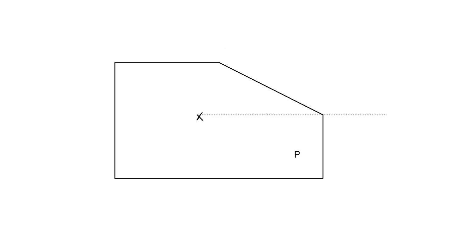
Figure 3. Drawn inside $B_{k}$ with the dashed ray representing the defining monodromy invariant ray

Proposition 8.5.

The restriction map

$$\mathcal{F}_{k}(S)\to\mathcal{F}_{k}(X)=\mathcal{O}_{0}(hull(E_{+}^{-1}(X)))$$

has in its image the element with formal expression $\xi.$

We first finish the proof of Proposition 8.4 using this statement.

Proof of Proposition 8.4.

Take an element $A\in\mathcal{F}_{k}(S)$ which has image $A_{X}=\xi$ under the identification $\mathcal{F}_{k}(X)=\mathcal{O}_{0}(hull(E_{+}^{-1}(X)))$ as in the statement of Proposition 8.5.

Restrict $A$ to either the upper edge $U$ or the lower edge $L$ of $P$. Using the left side of Diagram (48), we obtain elements $A_{U}\in\mathcal{O}_{0}(E_{+}^{-1}(U))$ and $A_{L}\in\mathcal{O}_{0}(E_{+}^{-1}(L))$. The formal expression for both of these elements is $\xi$.

Now use the upper and the lower wall-crossing isomorphisms to get elements in $A_{U}^{\prime}\in\mathcal{O}_{0}(hull(E_{-}^{-1}(U)))$ and $A_{L}^{\prime}\in\mathcal{O}_{0}(hull(E_{-}^{-1}(L)))$. We a priori know that both of these elements have to be restrictions of $A_{Y}\in\mathcal{O}_{0}(hull(E_{-}^{-1}(Y)))$ and in particular they have to have the same formal expression.

Writing this down using Proposition 8.3 we obtain

$$\xi\cdot(1+a_{1}\eta+a_{2}\eta^{2}+\ldots)=\xi\cdot\eta^{k}(1+b_{1}\eta^{-1}+b_{2}\eta^{-2}+\ldots).$$

It is easy to see that one can cancel $\xi$ from this relation. Indeed, we can restrict to a polygon where $\xi$ is invertible. The claim follows.

∎

Corollary 8.6.

The wall-crossing isomorphisms (both!) are given by

$$\eta\mapsto\eta,\xi\mapsto\xi(1+\eta)^{k}.$$

Proof.

For $k=1$, we uniquely determine the wall-crossing transformations from equation (62). For $k>1$, (62) does not have a unique solution, but notice that we can resolve the the $k$-fold singularity into $k$ simple nodal singularities lying on one monodromy invariant line by nodal sliding. This can be achieved by modifying $\pi_{k}$ in a small neighborhood of $\pi_{k}^{-1}(0)$, and in particular does not modify $\pi_{k}^{-1}(S)\subset M_{k}$ as a set or its relative $SH$. For this resolved singularity the wall crossing around all $k$ singularities is the same as the wall crossing around the unresolved one, and it factors as a $k$-fold iteration of the wall crossing isomorphism for the case $k=1$.

∎

Finally, we can prove Theorem 6.1.

Proof of Theorem 6.1.

As commented in Section 6.2 this amounts to matching the A- and B- side wall crossing. The formula for the B-side wall crossing is given in Proposition 3.10, which matches with Corollary 8.6. ∎

8.1. Proof of Proposition 8.5

Let us now prove the intermediary Proposition 8.5

Proof of Proposition 8.5.

Let $L$ be the edge of $X$ on the left. By functoriality with respect to inclusions and our knowledge of the restriction map $\mathcal{O}_{0}(hull(E_{+}^{-1}(X)))\to\mathcal{O}_{0}(E_{+}^{-1}(L))$ it suffices to prove that the restriction map to $L$ contains $\xi$, where we identified $\mathcal{F}_{k}(L)$ with $\mathcal{O}_{0}(E_{+}^{-1}(L))$ via the locality isomorphism as well.

A Hamiltonian $H$ is called $Q$-admissible for a subset $Q\subset B_{k}$ if $H<0$ on $\pi_{k}^{-1}(Q)$. A dissipative $H$ is called $\xi$-full if $\xi$ is in the image of the natural map $HF^{0}(H;\Lambda)\to SH^{0}_{M_{k}}(\pi_{k}^{-1}(L),\Lambda)=\mathcal{F}_{k}(L)$.

It suffices to show that there is an $S$-admissible Hamiltonian $H$ which is $\xi$-full. Indeed, the map $HF^{0}(H;\Lambda)\to\mathcal{F}_{k}(L)$ factors through the restriction map $\mathcal{F}_{k}(S)\to\mathcal{F}_{k}(L)$.

Let $B_{+}$ be the image of $E_{+}$ and $M_{+}:=\pi_{k}^{-1}(B_{+})$. A function $h:B_{k}\to{\mathbb{R}}$ is said to be convex on the left if $dh(e_{1})\geq 0$ on the eigenray $B_{k}\setminus B_{+}$ and on $B_{+}$ any co-vector $\nu$ with $\nu(e_{1})<0$ is obtained at most once as $dh_{b}$ for some $b\in B_{+}$, using the canonical identification of the cotangent spaces of points in $B_{+}$

For a function $h$ which is convex on the left we show now that if the level sets are sufficiently close to being rectangular in a neighbourhood of $L$ we have the following property. Equip $M$ with a $S$-compatible primitive (given by Euler primitive outside an open subset whose closure is contained in the interior of $S$). Consider the homology class $a$ in $H_{1}(M_{+},\mathbb{Z})$ given by the primitive covector (called $-e_{1}^{\vee}$) of the left edge pointing out of $S$. Let $\tilde{a}$ be its image in $H_{1}(M,\mathbb{Z})$. Then if $h$ has a $1$-periodic orbit $\gamma$ corresponding to $-e_{1}^{\vee}$, this orbit maximizes action among all orbits in the class $\tilde{a}$. To see this note the action of an orbit representing $e_{1}+ne_{2}^{\vee}$ is arbitrarily close to $-\lambda_{1}-|n|\lambda_{2}$ where $\lambda_{1}$ is the distance from the origin to $L$ and $\lambda_{2}$ is half the length of $L$ by Proposition 5.3 (using the flat metric in the domain of $E^{+}$).

Call a convex from the left $h$ which has sufficiently large slope to the left of $L$ and with level sets sufficiently close to rectangular for the property of the previous paragaraph to hold well-behaved. It is straightforward that we can construct acceleration data for $L$ which consist of well behaved Hamiltonians.

Given $F:M_{k}\times S^{1}\to\mathbb{R}$ that is an appropriate small time dependent perturbation of $f\circ\pi_{k}$ for a well behaved $f$, let $\gamma^{f}$ be the $1$-periodic orbit corresponding to the negative of $e_{1}^{\vee}$ in degree $0$. By standard Morse-Bott considerations, the only possible contributions to the differential of $\gamma^{f}$ are those connecting it to degree $1$ periodic orbits which don’t arise from the perturbation of $-e_{1}^{\vee}$. By action considerations we conclude that $\gamma^{f}$ is a cycle. Fix such $H,G$ so that $H$ is $S$-admissible and $G$ is $L$-admissible. Assume that a neighborhood of $\gamma^{H}$ coincides with a neighborhood of $\gamma^{G}$ and that $H$ and $G$ coincide there. Then $\gamma^{H}$ maps precisely to $\gamma^{G}$. Indeed, we have the constant solution, and we can have no other by the action minimization.

To conclude, we turn to show that at least for carefully chosen $G$ and almost complex structures, the generator $\gamma^{G}$ maps to a non-zero scalar multiple of $\xi$. By nodal sliding to the right (similar to the argument in locality for complete embeddings) we can assume that any relevant Floer trajectory with $\gamma^{G}$ as input with energy $\leq 1$ is contained in a fixed compact neighbourhood $K$ of $\pi^{-1}_{k}(L)$ inside $M_{+}$. Thus, up to $O(1)$ we can guarantee that $\gamma^{G}$ maps to $T^{\epsilon}\xi$ where $\epsilon<1$. To see the last point let $G_{loc}$ be an extension of $G|_{K}$ to $M_{0}$ which is still convex from the left. Then at least for $G_{loc}$ large enough we know that $\xi$ is in the image of the map $HF^{*}(G_{loc})\to SH^{*}_{M_{0}}(\pi^{-1}(L))$. But the only thing that can map to $\xi$ is $\gamma^{G}$. We now rule out the possibility of an $O(1)$ correction. Such a correction would amount to a continuation trajectory from $\gamma^{G}$ to some orbit $\delta$ of some well behaved Hamiltonian $G^{\prime}>G$ so that $\delta$ is in the class $\tilde{a}$ in $M$ but not in $M^{+}$. By definition of well behavedness such a $\delta$ has lower action and such a trajectory is impossible.

∎

Remark 8.7.

Let us explain what happened a posteriori. The $A$-side wall crossing maps as defined by Diagram (48) gives us an isomorphism of the rigid analytic spaces

$$(\Lambda^{*})^{2}\setminus\{val(\eta^{-})=0\}\to(\Lambda^{*})^{2}\setminus\{val(\eta^{+})=0\}.$$

This is a morphism between two disconnected spaces and it appears that we have two entirely independent maps. But it turns out that in fact this map extends to an isomorphism

$$(\Lambda^{*})^{2}\setminus\{\eta^{-}=-1\}\to(\Lambda^{*})^{2}\setminus\{\eta^{+}=-1\}.$$

If we knew this fact a priori, then Proposition 8.4 would follow as both maps (and in particular the pullback of the regular function $\xi^{+}$) are determined by this one map. In fact our results prove that it is the restriction of the transition map from Proposition 3.10.

Our monodromy argument is a replacement of this point. Its intuition is the knowledge that the function $\xi^{+}$ extends to a function $Y_{1}^{an}$ and hence maybe we should use the mirror of this global function to obtain the desired relationship between how the mirror of $\xi^{+}$ transforms under the two wall crossing transformations.

9. Hartogs’s property

Our goal in this section is to prove the following statement, which will allow us to extend the isomorphism of Theorem 6.1 to all of $B_{k}$.

Proposition 9.1.

Let $P\subset B_{k}$ be an admissible convex polygon containing a node in its interior. Then, the restriction map

$$\mathcal{F}_{k}(P)\to\mathcal{F}_{k}(\partial P)$$

is an isomorphism.

Recall that the same statement holds if we replace $\mathcal{F}_{k}$ with $\mathcal{O}_{k}$, see Proposition 3.17. The rough idea of the proof is that one can choose the acceleration data for $\partial P$ and $P$ so that in a large region where the degree $0$ orbits of the Hamiltonians are contained the acceleration data are exactly the same. We start with an abstract lemma.

Lemma 9.2.

Let $C\to D$ be a chain map of non-negatively graded chain complexes. Assume that $C^{0}\to D^{0}$ is an isomorphism and $C^{1}\to D^{1}$ is injective. Then, $H^{0}(C)\to H^{0}(D)$ is an isomorphism.

Proof.

For a formal proof, truncate the complexes at degree $2$ and consider the long exact sequence. ∎

Lemma 9.3.

Let us take a map of $1$-rays over the Novikov ring $\Lambda_{\geq 0}$

(67)

Assume that each of these chain complexes are non-negatively graded, in degrees $0$ and $1$ they are free of finite rank,

$$f_{i}^{0}:\mathcal{C}_{i}^{0}\otimes\Lambda_{\geq 0}/\Lambda_{>0}\to\mathcal{C}_{0}^{{}^{\prime}1}\otimes\Lambda_{\geq 0}/\Lambda_{>0}$$

is an isomorphism,

$$f_{i}^{1}:\mathcal{C}_{i}^{1}\otimes\Lambda_{\geq 0}/\Lambda_{>0}\to\mathcal{C}_{i}^{{}^{\prime}1}\otimes\Lambda_{\geq 0}/\Lambda_{>0}$$

is injective and both $H^{0}(\widehat{tel}(\mathcal{C}))$ and $H^{0}(\widehat{tel}(\mathcal{C}^{\prime}))$ have finite torsion.

Then, the induced map

$$H^{0}(\widehat{tel}(\mathcal{C}))\to H^{0}(\widehat{tel}(\mathcal{C}^{\prime}))$$

is an isomorphism.

Proof.

We have the commutative diagram:

(72)

and, under the finite torsion assumption, the vertical maps are isomorphisms by [9, Proposition 1.2].

Therefore, it suffices to show that

$$H^{0}(\mathcal{C}_{i}/T^{r}\mathcal{C}_{i})\to H^{0}(\mathcal{C}_{i}^{\prime}/T^{r}\mathcal{C}_{i}^{\prime})$$

is an isomorphism for every $r\geq 0$ and $i=1,2,\ldots$. Fix an $i$ and $r$ for the rest of the argument.

Now, by Nakayama’s lemma, we see that

$$f_{i}^{0}:\mathcal{C}_{i}^{0}\otimes\Lambda_{\geq 0}/\Lambda_{>r}\to\mathcal{C}_{i}^{{}^{\prime}0}\otimes\Lambda_{\geq 0}/\Lambda_{>r}$$

is an isomorphism.

Note that, moreover,

$$f_{i}^{1}:\mathcal{C}_{i}^{1}\otimes\Lambda_{\geq 0}/\Lambda_{>r}\to\mathcal{C}_{i}^{{}^{\prime}1}\otimes\Lambda_{\geq 0}/\Lambda_{>r}$$

preserves the module norms and hence is injective for all $r\geq 0$. Here we are also using that $\mathcal{C}_{i}^{1}$ is free to conclude that the module semi-norms are in fact norms.

Finally, we use Lemma 9.2.

∎

Proof of Proposition 9.1.

We construct acceleration data for $P$ and $\partial P$ and homotopy data for the restriction map so that the hypotheses of the previous lemma hold.

Let us call a smooth function $f:B_{1}\to\mathbb{R}$ strongly non-degenerate if

• In a neighborhood of the node $f$ only depends on the monodromy invariant integral affine coordinate $u$ and $0<\frac{\partial f}{\partial u}(0)<1$.

• The Hessian

  (73) $$\left(\frac{\partial^{2}f}{\partial q_{i}\partial q_{j}}(b)\right)$$

  with respect to an (and hence any) integral affine coordinate system $q_{1},q_{2}$ is non-degenerate for every $b\in B^{reg}_{1}$ such that $df_{b}\in T_{\mathbb{Z}}^{*}B$.

• It is dissipative for some geometrically bounded almost complex structure.

Note that the first bullet point implies that the only $1$-periodic orbit of the Hamiltonian $f\circ\pi_{1}$ which lies on the nodal fiber $\pi_{1}^{-1}(0)$ is the constant orbit at the focus-focus singularity. Moreover, the Morse index of this critical point of $f\circ\pi_{1}$ is $2$. To see this note that in a neighborhood of the singular point there are complex valued coordinates $z_{1},z_{2}$ such that $u\circ\pi_{1}$ is the map $(z_{1},z_{2})\mapsto|z_{1}|^{2}-|z_{2}|^{2}$.

Using the strategy described at the end of Section 6.1 (label!), we choose

• a sequence of strongly non-degenerate smooth functions $f_{1}<f_{2}<\ldots$ and $g_{1}<g_{2}<\ldots$

• a sequence of compact domains $D_{1}\subset D_{2}\subset\ldots$ inside $B_{1}$

such that

• $f_{1}<f_{2}<\ldots$’s form a cofinal sequence among functions that are negative on $P$

• $g_{1}<g_{2}<\ldots$’s form a cofinal sequence among functions that are negative on $\partial P$

• $f_{i}=g_{i}$ outside of $D_{i}$ for every $i\geq 0$

• $f_{i}$ is $C^{2}$-small inside $D_{i}$.

• $g_{i}$ is so that if $(dg_{i})_{b}\in T_{\mathbb{Z}}^{*}B$ for $b\in D_{i}$, then the Hessian from (73) is not positive definite.

We carefully perturb the Morse-Bott families of orbits with the condition that outside of $D_{i}$ we use the same perturbations for both $f_{i}$ and $g_{i}$. After choosing the relevant monotone interpolations, the conditions of Lemma 9.3 are easily checked. ∎

We finally prove Theorem 1.8

Proof of Theorem 1.8.

We want to show that we can extend the isomorphism of Theorem 6.1. By another application of Lemma 2.1, it suffices to extend it to admissible convex polygons containing the node. We define these isomorphisms by the diagram

(78)

where the vertical maps are given by Propositions 9.1 and 3.17, for any such $P\subset B_{k}.$

We need to check that, for an admissible convex polygon $Q\subset P\subset B_{k}$,

(83)

commutes.

First, note that when $Q\subset\partial P$, this is immediate as the restriction maps factor through $\partial P$. Now assume that $Q\subset P$ intersects $\partial P$ and let $q\in Q\cap\partial P$. Then $q\in\partial Q$. Consider the diagram

(88)

We already know the outer rectangle and the square on the right commute. Noting that $\mathcal{O}_{k}(Q)\to\mathcal{O}_{k}(\{q\})$ is injective finishes the proof. This injectivity is immediate (see [3, Lemma 10]) from the fact that $p_{k}^{-1}(\{q\}\subset p_{k}^{-1}(Q)$ is an affinoid (in fact rational) subdomain, which was shown in the proof of Proposition 3.14.

Finally, assume that $Q$ is arbitrary. We can find an admissible convex polygon $Q^{\prime}\subset P$ which intersects both $Q$ and $\partial P$. Let $q^{\prime}\in\partial Q^{\prime}\cap\partial Q$. Both squares in the diagram

(93)

commute so the composition square also commutes. We finish this time using the injectivity of $\mathcal{O}_{k}(Q)\to\mathcal{O}_{k}(\{q^{\prime}\}).$

∎

10. Construction of mirrors

10.1. Symplectic cluster manifolds

Let $\mathcal{R}$ be an eigenray diagram. As explained in Section 7 of [9], one can associate to $\mathcal{R}$ a symplectic manifold $M_{\mathcal{R}}$ together with a nodal Lagrangian fibration $\pi_{\mathcal{R}}:M_{\mathcal{R}}\to B_{\mathcal{R}}$. The pre-image of an admissible polygon containing a singular point with monodromy $A_{k}$ is modeled on $\pi_{k}:M_{k}\to B_{k}$. There are some choices involved in the construction near each node but by abuse of notation we will shall not distinguish them.

A symplectic cluster manifold is symplectic manifold which is symplectomorphic to $M_{\mathcal{R}}$ for some eigenray diagram $\mathcal{R}$. A given symplectic cluster manifold may have multiple eigenray diagram representations as a result of nodal slide and branch move operations on eigenray diagrams. See Section 7.2 of [9].

The following is Proposition 7.17 of [9].

Proposition 10.1.

Symplectic cluster manifolds are geometrically of finite type.

If $M$ is a symplectic cluster manifold, then $c_{1}(M)=0$ and there is a preferred trivialization up to homotopy of $\Lambda^{n}T_{\mathbb{C}}M,$ which makes the regular fibers of any associated $\pi_{\mathcal{R}}:M_{\mathcal{R}}\to B_{\mathcal{R}}$ have Maslov homomorphism $\pi_{1}(T^{2},\star)\to\mathbb{R}$ zero. We use this grading datum in defining relative $SH$ without further mention.

For a small admissible polygon we say it has multiplicity $k>0$ if it contains a singular value of multiplicity $k$. If it contains no singular value we say it has multiplicity $0$.

Proposition 10.2.

Let $P\subset B_{\mathcal{R}}$ be a small admissible polygon of multiplicity $k$. Then there exists a complete embedding $\iota:M_{k}\to M_{\mathcal{R}}$, a convex admissible polygon $P_{0}\subset B_{k}$, and an integral affine embedding $f:U\to B_{\mathcal{R}}$ from neighborhood of $P_{0}$ so that

• $f(P_{0})=P$

• $\pi_{\mathcal{R}}^{-1}(P)\subset\iota(M_{k})$

• $\pi_{\mathcal{R}}\circ\iota|_{\pi_{k}^{-1}(P_{0})}=f\circ\pi_{k}$.

Proof.

If the multiplicity is $k>0$ we can choose Lagrangian tails $L_{i}$ lying over each ray not emanating from the singular value inside $P$. The complement of these tails is symplectomorphic to $M_{k}$ according to [9, Theorem 1.8]. Moreover, this symplectomorphism can be taken to intertwine the Lagrangian fibrations away from arbitrarily small neighborhoods of the removed rays. If the multiplicity is $0$ and $P$ intersects no rays we can again do the same thing. If $P$ meets some ray $l$ then by removing tails over rays which don’t meet $P$ the complement is symplectomorphic to $M_{k}$ in a fibration preserving manner near $P$. We can then perform a branch move on $l$, which has no effect on the fibration, and reduce to the previous case. ∎

We can now prove the five properties listed in Theorem 1.5.

Proof of Theorem 1.5.

The locality isomorphism of Theorem 6.3 and Proposition 10.2 reduce the result to the same statements for $\mathcal{F}_{k}$ on $B_{k}$. Theorem 1.8 reduces it to $\mathcal{O}_{k}$ on $B_{k},$ which is covered by Corollary 3.16. ∎

10.2. Gluing

For $P$ a small admissible polygon in $B_{\mathcal{R}}$, we consider the affinoid domains

$$M(P):=M(\mathcal{F}_{\mathcal{R}}(P)).$$

Let us denote by

$$\iota_{Q\subset P}:M(Q)\to M(P)$$

the maps induced by the restriction maps.

We denote the collection of all small admissible polygons in $B_{\mathcal{R}}$ by $\{P_{i}\}_{i\in I}$. Let us define, for each pair $i,j\in I,$ the affinoid subdomains

$$U_{ij}:=\iota_{P_{i}\cap P_{j}\subset P_{i}}(M(P_{i}\cap P_{j})).$$

Then, for all $i,j\in I$, we automatically obtain the isomorphism

$$\psi_{ij}:=\iota_{P_{i}\cap P_{j}\subset P_{j}}\circ\iota_{P_{i}\cap P_{j}\subset P_{i}}^{-1}:U_{ij}\to U_{ji}.$$

Lemma 10.3.

For $i,j,k\in I,$ we have

$$\psi_{ij}(U_{ij}\cap U_{ik})\subset U_{ji}\cap U_{jk}.$$

Proof.

Note that we have

$$U_{ij}\cap U_{ik}=im(\mathcal{M}(P_{i}\cap P_{j}\cap P_{k}))$$

inside $\mathcal{M}(P_{i})$ by the strong cocycle condition, and the map $\iota_{P_{i}\cap P_{j}\cap P_{k}\subset P_{i}}$ is the same as

$$\iota_{P_{i}\cap P_{j}\subset P_{i}}\circ\iota_{P_{i}\cap P_{j}\cap P_{k}\subset P_{i}\cap P_{j}}$$

by the presheaf property of restriction maps.

Therefore, we have a canonical commutative diagram

(98)

where the image of $M(P_{i}\cap P_{j}\cap P_{k})$ in $U_{ij}$ and $U_{ji}$ is equal to $U_{ij}\cap U_{ik}$ and $U_{ji}\cap U_{jk},$ respectively. The proof is immediate. ∎

For $i,j,k\in I,$ let us give the name

$$\psi_{ijk}:U_{ij}\cap U_{ik}\to U_{ji}\cap U_{jk}$$

to the map obtained by restricting $\psi_{ij}$.

Lemma 10.4.

The collection of maps $\psi_{ij}$ satisfies $\psi_{ij}\circ\psi_{ji}=id$, $\psi_{ii}=id$ and the cocycle condition

$$\psi_{ijk}=\psi_{kji}\circ\psi_{ikj}.$$

Proof.

The first two are obvious. The cocycle condition follows from the commutativity of the diagram of isomorphisms:

(103)

∎

As in [3, Proposition 5] we now define the rigid analytic space by gluing $M(P_{i})$ along $U_{ij}$’s using $\psi_{ij}$’s. As a set

(104) $$\mathcal{Y}_{\mathcal{R}}=\coprod_{i\in I}M(P_{i})/\sim$$

where $\sim$ is the relation $x\in U_{ij}\sim\psi_{ij}(x)\in U_{ji}$.

Note that by construction there are canonical embeddings of each $\mathcal{M}(P_{i})$ into $\mathcal{Y}_{\mathcal{R}}$ and we call their images (which are admissible opens) $X_{i}\subset\mathcal{Y}_{\mathcal{R}}.$ If $P_{i}\subset P_{j}$, then $X_{i}\subset X_{j}$.

We now want to construct a map $p_{\mathcal{R}}:\mathcal{Y}_{\mathcal{R}}\to B_{\mathcal{R}}$ using the properties listed in Theorem 1.5.

Proposition 10.5.

Let $y\in\mathcal{Y}_{\mathcal{R}}$. Denote by $I_{y}\subset I$ the set of indices for which $P_{i}$ is a small admissible polygon such that $y\in X_{i}$. Then the set

$$\bigcap_{i\in I_{y}}P_{i}\subset B_{\mathcal{R}}$$

is a singleton $\{b_{y}\}$.

Proof.

We first claim that there is a sequence of small admissible polytopes

$$P_{i(1)}\supset P_{i(2)}\supset\ldots$$

such that

• $i(k)\in I_{y}$ for all $k\geq 1$.

• $\bigcap_{k\geq 1}P_{i(k)}$ is a singleton.

Note that we have an explicit PL isomorphism $\mathbb{R}^{2}\simeq B_{\mathcal{R}}$ by construction. Let us use the flat metric on $\mathbb{R}^{2}$ to equip $B_{\mathcal{R}}$ with a metric space structure.

By construction $I_{y}$ is non-empty. Let $i(1)\in I_{y}$. Partition $P_{i(1)}=\bigcup_{k=1}^{n}P_{j(k)}$ into admissible convex polygons (which are automatically small) with half the diameter. Using the independence property we know that $y\in X_{j(k)}$ for some $k$. We let $i(2)=j(k)$ and thus continue inductively. The polygons $P_{i(k)}$ are compact in the standard topology on $B_{\mathcal{R}}$ so we deduce that the intersection $\bigcap_{k\geq 1}P_{i(k)}$ is non-empty and of $0$ diameter. That is, a singleton.

It follows, first, that the intersection $\bigcap_{i\in I_{y}}P_{i}$ has at most one element. It remains to show non-emptyness. Let $b_{y}$ be the unique element in $\bigcap_{k\geq 1}P_{i(k)}$. Let $i\in I_{y}$ and assume by contradiction that $b_{y}\not\in P_{i}$. Then for $k$ large enough, $P_{i}\cap P_{i(k)}=\emptyset$. But then we cannot have $y\in X_{i}\cap X_{i(k)}$ by the gluing construction. This contradiction completes the proof. ∎

We thus define a canonical map

$$p_{\mathcal{R}}:\mathcal{Y}_{\mathcal{R}}\to B_{\mathcal{R}}$$

by $y\to b_{y}$.

Lemma 10.6.

For any small admissible polygon $P_{i}$ we have $p_{\mathcal{R}}^{-1}(P_{i})=X_{i}$ .

Proof.

For $y\in X_{i}$ we have $b_{y}\in P_{i}$ by construction. So $p_{\mathcal{R}}(X_{i})\subset P_{i}$. Conversely, suppose $b\in P_{i}$. We want to show that $p_{\mathcal{R}}^{-1}(b)\subset X_{i}$. Let $y\in p_{\mathcal{R}}^{-1}(b),$ that is $b_{y}=b.$

Let $P_{j}$ be any small admissible polygon such that $y\in X_{j}$. Let $P_{k}=P_{i}\cap P_{j}$. Note that $b$ is contained in $P_{k}$. Then we claim that $y\in X_{k}$. Assuming $y\notin X_{k}$, by the separation property, there is a $P_{l}\subset P_{j}$ which does not contain $b$ so that $y\in X_{l}$. This contradicts the construction of $b=b_{y}$. Therefore, we have that $y\in X_{k}\subset X_{i}$.

∎

Proposition 10.7.

If $P\subset B_{\mathcal{R}}$ is a small admissible polygon of multiplicity $k$ there is a commutative diagram of sets

(109)

where the upper horizontal arrow is an analytic embedding and the lower arrow is a nodal integral affine embedding.

Proof.

By Lemma 10.6 we have $p_{\mathcal{R}}^{-1}(P_{i})=X_{i}\simeq\mathcal{M}(P_{i})$. The upper horizontal arrow is the one induced by the locality isomorphism and the lower arrow is the inverse of the map $f$ from Lemma 10.2 restricted to $f^{-1}(P)$. It remains to show commutativity.

For this note, that for $P_{i}\subset P_{j}$ admissible polygons, locality and the isomorphism of Theorem 1.8 intertwine the inclusion $\mathcal{M}(P_{i})\to\mathcal{M}(P_{j})$ with the inclusion $p_{k}^{-1}(P_{i})\to p_{k}^{-1}(P_{j})$. Second, for any $y\in Y_{k}$ we have tautologically that $p_{k}(y)=\cap_{i:y\in p_{k}^{-1}(P_{i})}P_{i}$ where $i$ runs over all small admissible polygons in $B_{k}$. The commutativity thus follows by construction of $p_{\mathcal{R}}$. ∎

Proof of Theorem 1.1.

We have already constructed $\mathcal{Y}_{\mathcal{R}}$ with its map $p_{\mathcal{R}}\to B_{\mathcal{R}}$. That $p_{\mathcal{R}}$ is a Stein continuous map follows from Lemma 10.6 and the properties of the gluing construction of analytic spaces. Let us denote the structure sheaf of $\mathcal{Y}_{\mathcal{R}}$ by $\mathcal{O}_{\mathcal{R}}.$

By construction and Lemma 10.6, for a small admissible polygon $P$,

$$(p_{\mathcal{R}})_{*}\mathcal{O}_{\mathcal{R}}(P)=\mathcal{F}_{\mathcal{R}}(P).$$

Invoking Lemma 2.1 we obtain the desired isomorphism of sheaves of algebras $\mathcal{F}_{\mathcal{R}}\simeq p_{\mathcal{R}}^{*}\mathcal{O}_{\mathcal{R}}$.

Let us now start proving the numbered assertions. The items (1) and (2) follow immediately from Proposition 10.7 and the discussion in Section 3.2 for $p_{k}:Y_{k}\to B_{k}$. For item (3), we in addition need Proposition 3.18 and the fact that $\Omega_{0}$ is invariant under the action of the integral affine transformations $SL(2,\mathbb{Z})\ltimes\mathbb{R}^{2}$ on $Y_{0}^{an}=(\Lambda^{*})^{2}$.

Note that if we take a cover of $B_{\mathcal{R}}$ by small admissible polygons, we can construct $\mathcal{Y}_{\mathcal{R}}$ by gluing only the corresponding affinoid domains because of the invariance property. If the cover is sufficiently fine, namely if for every point of $B_{\mathcal{R}}$ there is a descending chain of members of the cover with intersection precisely equalling that point, then we can construct $p_{\mathcal{R}}$ only using this cover. Items (4) and (5) follow from this point.

For (4), we note that $B_{\mathcal{R}_{1}}$ and $B_{\mathcal{R}_{2}}$ are canonically identified as nodal integral affine manifolds and we use the cover by the admissible polygons which are small with respect to both eigenray representations.

For (5), first assume that we can find a small admissible polygon in $B_{\mathcal{R}_{1}}$ which contains the nodal slide locus in its interior. We consider the covers of $B_{\mathcal{R}_{1}}$ and $B_{\mathcal{R}_{2}}$ (canonically identified by a PL isomorphism) by this small admissible polygon and all the small admissible polygons which do not intersect the nodal slide locus. Clearly, the resulting rigid analytic spaces are the same. Moreover, we see that the isomorphism respects the fibrations outside of the nodal slide locus. The general case follows by iterating this step.

Finally, for (6), it suffices to note that both sides can be defined as an inverse limit over the preimage of an exhaustion of $B_{\mathcal{R}}$ by admissible polygons.

∎

Remark 10.8.

Our proof of the first three bullet points rely on a computation (not just properties) and is ad-hoc. At least when all the multiplicities are $1$, we expect to be able to give a much more conceptual proof based on the fact that there is a Lagrangian section $L$ satisfying the local generation property after recasting the construction of $\mathcal{Y}_{\mathcal{R}}$ using the relative Lagrangian Floer homology of $L$.

The intrinsic meanings of (2) and (3) are clear. One might consider replacing (1) with the statement that $p_{\mathcal{R}}$ is the projection to the essential skeleton defined using the canonical volume form on $\mathcal{Y}_{\mathcal{R}}$.

11. Future work

11.1. Higher dimensions

In this section we want to briefly explain how our methods would extend to higher dimensions. Let us start with a generalization that is essentially straightforward.

Any triple $(\mu,f,Z)$, where

• $\mu:\mathbb{R}^{n}\to\mathbb{R}$ an integral affine function

• $f\in\mathbb{Z}^{n}$ such that $d\mu(f)=0$

• a properly embedded connected codimension $1$ smooth submanifold $Z$ of

  $$H:=\{x\in\mathbb{R}^{n}\mid\mu(x)=0\}$$

  which is transverse to $f$ everywhere

defines a subset $S(\mu,f,Z)$ of $\mathbb{R}^{n}$ by considering the closure of the $f$-positive side of $Z$ inside $H$.

Given $(\mu,f,Z)$ inside $\mathbb{R}^{n}$ we can define a nodal integral affine manifold with the singular locus $Z$ by regluing a connected neighborhood of $S:=S(\mu,f,Z)$ by the identity on the $\mu(x)>0$ side and by the transvection

(110) $$v\mapsto v-\mu(v)\cdot f.$$

on the other.

We define a shear-cut diagram $\mathcal{R}$ in $\mathbb{R}^{n}$ as a finite collection of such triples $(\mu_{i},f_{i},Z_{i}),i\in I$ such that $S_{i}:=S(\mu_{i},f_{i},Z_{i})$ are pairwise disjoint. Given a shear cut locus $\mathcal{R}$, we can define a Lagrangian fibration $\pi_{\mathcal{R}}:M_{\mathcal{R}}\to B_{\mathcal{R}}$ with only focus-focus singularities such that the induced nodal integral affine structure is isomorphic to the one induced on $\mathbb{R}^{n}$ by $\mathcal{R}$ [2].

We have analogues of the nodal slide and branch cut operations. For nodal slides, we can isotope $Z_{i}$ inside $H_{i}=\{\mu_{i}(x)=0\}$ as a properly embedded smooth submanifold keeping it transverse to $f_{i}$. This does not change $M_{\mathcal{R}}$ but modifies the fibration $\pi_{\mathcal{R}}$. Assuming that $H_{i}$ is disjoint from all the other $S_{j}$’s, we can apply a branch move by replacing $f_{i}$ with $-f_{i}$. This only changes how we represent our Lagrangian fibration using a shear-cut diagram.

Let us identify $B_{\mathcal{R}}$ with $\mathbb{R}^{n}$ using the canonical PL homeomorphism and denote the singularity locus $\bigcup_{i\in I}Z_{i}$ by $Z$. We now start assuming that $Z_{i}$ are in fact affine. This means that there are neighborhoods of $Z_{i}$ which are for some $k_{i}$ isomorphic to a neighborhood of $\mathbb{R}^{n-2}\times\{\text{node}\}$ inside $\mathbb{R}^{n-2}\times B_{k_{i}}.$ Let us fix such isomorphisms and call this data a framing.

We define an admissible convex polygon in $B_{\mathcal{R}}$ to be a convex rational polygon if it does not intersect $Z$, and if it does intersect, as a product of admissible convex rational polygons inside $\mathbb{R}^{n-2}$ and $B_{k_{i}}$ with respect to a fixed framing.

Using locality for complete embeddings, Kunneth theorem e.g. [8, Theorem 10.6] and some torsion analysis it should be easy to prove Theorem 1.5 and then construct a mirror $p_{\mathcal{R}}:\mathcal{Y}_{\mathcal{R}}\to B_{\mathcal{R}}$.

We can go further and consider more complicated constructions. To illustrate the idea let us focus on dimension $3$. In that case we consider $(\mu,\Delta,Z)$ where $\mu:{\mathbb{R}}^{3}\to{\mathbb{R}}^{2}$ is an integral affine map, $\Delta\subset{\mathbb{R}}^{2}$ is a tropical curve, and $Z\subset\mu^{-1}(\Delta)$ is a codimension $1$-graph projecting bijectively onto $\Delta$ under $\mu$. We label the two components of $\mu^{-1}(\Delta)\setminus Z$ by $j\in\{\pm\}$, and denote the closure by $S_{j}(\mu,\Delta,Z)$. Assume that we are given $\mathcal{R}$, a collection of $(\mu_{i},\Delta_{i},Z_{i})$ and a choice of signs $j_{i}$ such that $S_{j_{i}}(\mu_{i},\Delta_{i},Z_{i})$ are pairwise disjoint. Then, we can form by the same method as above an integral affine manifold with nodal singularities on the edges. At each vertex we get the singular integral affine structure of the positive vertex. Accordingly we can form a symplectic manifold $M_{\mathcal{R}}$ by gluing a neighborhood of the singular fibers of the Gross-fibration corresponding to $\Delta$. See [9] for a more detailed discussion of the local models. We expect the methods of this paper to extend to allow the proof of Theorem 1.5 and moreover to compute the local models.

References

- [1] Sergey Barannikov and Maxim Kontsevich. Frobenius manifolds and formality of Lie algebras of polyvector fields. International Mathematics Research Notices, 1998(4):201–215, 1998.
- [2] Ricardo Castano Bernard and Diego Matessi. Lagrangian 3-torus fibrations. Journal of Differential Geometry, 81(3):483–573, 2009.
- [3] Siegfried Bosch. Lectures on formal and rigid geometry, volume 2105. Springer, 2014.
- [4] Ricardo Castano-Bernard, Diego Matessi, and Jake P Solomon. Symmetries of Lagrangian fibrations. Advances in mathematics, 225(3):1341–1386, 2010.
- [5] Brian Conrad. Several approaches to non-archimedean geometry. In p-adic geometry, pages 9–63, 2008.
- [6] Manfred Einsiedler, Mikhail Kapranov, and Douglas Lind. Non-archimedean amoebas and tropical varieties. 2006(601):139–157, 2006.
- [7] Kenji Fukaya, Yong-Geun Oh, Hiroshi Ohta, and Kaoru Ono. Lagrangian Floer theory on compact toric manifolds, I. Duke Mathematical Journal, 151(1):23–175, 2010.
- [8] Yoel Groman. Floer theory and reduced cohomology on open manifolds. arXiv preprint arXiv:1510.04265, 2015.
- [9] Yoel Groman and Umut Varolgunes. Locality of relative symplectic cohomology for complete embeddings. arXiv preprint arXiv:2110.08891, 2021.
- [10] Walter Gubler. Tropical varieties for non-archimedean analytic spaces. Inventiones mathematicae, 169(2):321–376, 2007.
- [11] Paul Hacking and Ailsa Keating. Homological mirror symmetry for log Calabi-Yau surfaces. arXiv preprint arXiv:2005.05010, 2020.
- [12] Doris Hein. The Conley conjecture for irrational symplectic manifolds. Journal of Symplectic Geometry, 10(2):183–202, 2012.
- [13] Maxim Kontsevich and Yan Soibelman. Affine structures and non-archimedean analytic spaces. In The unity of mathematics, pages 321–385. Springer, 2006.
- [14] Myeonggi Kwon and Otto van Koert. Brieskorn manifolds in contact topology. Bulletin of the London Mathematical Society, 48(2):173–241, 2016.
- [15] Janko Latschev, Alexandru Oancea, and Mohammed Abouzaid. Free loop spaces in geometry and topology: including the monograph Symplectic cohomology and Viterbo’s theorem by Mohammed Abouzaid. European Mathematical Society, 2015.
- [16] Yu-Shen Lin. Correspondence theorem between holomorphic discs and tropical discs on K3 surfaces. Journal of Differential Geometry, 117(1):41–92, 2021.
- [17] Werner Luetkebohmert. On extension of rigid analytic objects. Muenster Journal of Mathematics.
- [18] Travis Mandel and Helge Ruddat. Tropical quantum field theory, mirror polyvector fields, and multiplicities of tropical curves. arXiv preprint arXiv:1902.07183, 2019.
- [19] Daniel Pomerleano. Intrinsic mirror symmetry and categorical crepant resolutions. arXiv preprint arXiv:2103.01200, 2021.
- [20] Joel Robbin and Dietmar Salamon. The Maslov index for paths. Topology, 32(4):827–844, 1993.
- [21] Hans Schoutens. Embedded resolution of singularities in rigid analytic geometry. In Annales de la Faculté des sciences de Toulouse: Mathématiques, volume 8, pages 297–330, 1999.
- [22] Paul Seidel. A biased view of symplectic cohomology. Current developments in mathematics, 2006(1):211–254, 2006.
- [23] Paul Seidel. Some speculations on pairs-of-pants decompositions and Fukaya categories. Surveys in Differential Geometry, 17(1):411–426, 2012.
- [24] Dmitry Tonkonog. String topology with gravitational descendants, and periods of Landau-Ginzburg potentials. arXiv preprint arXiv:1801.06921, 2018.
- [25] Dmitry Tonkonog and Umut Varolgunes. Super-rigidity of certain skeleta using relative symplectic cohomology. arXiv preprint arXiv:2003.07486, 2020.
- [26] Michael Usher. Hofer’s metrics and boundary depth. In Annales scientifiques de l’École Normale Supérieure, volume 46, pages 57–129, 2013.
- [27] Umut Varolgunes. Mayer-Vietoris property for relative symplectic cohomology. PhD thesis, Massachusetts Institute of Technology, 2018.
- [28] Umut Varolgunes. Mayer–vietoris property for relative symplectic cohomology. Geometry & Topology, 25(2):547–642, 2021.
- [29] Charles A. Weibel. An introduction to homological algebra, volume 38 of Cambridge Studies in Advanced Mathematics. Cambridge University Press, Cambridge, 1994.
- [30] Tony Yue Yu. Enumeration of holomorphic cylinders in log Calabi–Yau surfaces, II: Positivity, integrality and the gluing formula. Geometry & Topology, 25(1):1–46, 2021.
- [31] Hang Yuan. Family Floer program and non-archimedean SYZ mirror construction. arXiv preprint arXiv:2003.06106, 2020.