$p$-adaptive algorithms in Discontinuous Galerkin solutions to the time-domain Maxwell’s equations

Abstract

The Discontinuous Galerkin time-domain method is well suited for adaptive algorithms to solve the time-domain Maxwell’s equations and depends on robust and economically computable drivers. Adaptive algorithms utilize local indicators to dynamically identify regions and assign spatial operators of varying accuracy in the computational domain. This work identifies requisite properties of adaptivity drivers and develops two methods, a feature-based method guided by gradients of local field, and another utilizing the divergence error often found in numerical solution to the time-domain Maxwell’s equations. Results for canonical testcases of electromagnetic scattering are presented, highlighting key characteristics of both methods, and their computational performance.

1 Introduction

Mesh adaptive methods aim to efficiently allocate discrete degrees of freedom throughout a computational space. The finite element method and development of the popular Discontinuous Galerkin Finite Element Method (DGFEM) provides flexibility with non-conforming meshes having hanging nodes, and facilitates $p$-anisotropy, i.e. variation of degree of the basis polynomials across cells. Adaptive methods have been widely studied with initial ideas appearing in the works of Babuška and co-workers [1, 2, 3]. Broadly, adaptive methods are classified into three categories: those based on residuals or local error estimation [4, 5, 6], adjoint-based methods that estimate the error in a particular simulation output of interest as an objective functional [7, 8, 9, 10] and, the feature-based methods, recognized by easily computable indicators, often encoding identifiable physical quantities to be accurately resolved [11, 12, 13, 14]. Feature-based methods use readily computable response variables and their gradients like density or pressure gradients are classically approaches to identify regions of interest. The primary limitation these techniues is that the identified features may not show a direct relation with the underlying numerical discretization errors [4]. Also, the subjectivity involved due to their heuristic nature requires an expert user to devise effective feature-based schemes [15]. Adjoint-based methods eliminate these drawbacks to an extent, relying on numerical approximations of the adjoint problem to compute the error in a target functional. Despite being theoretically sound, these methods have not found widespread industrial application, owing to their high computational cost [16, 17]. Residual or error-based methods work towards making the mesh richer by estimating local sources of error. This approach has been shown to be computationally more economical than adjoint methods, and are autonomous [5]. Error estimation driven adaptive methods have found a lot of interest and a wide range of error estimation techniques and applications can be found in literature [4, 18, 19]. In hyperbolic problems, the two relevant numerical errors are discretization and truncation errors. The discretization error is advected downstream from under-resolved regions in space, unlike the truncation error, that acts as a local source [17]. The truncation error is related to the discretization error through the Discretization Error Transport equation (DETE) and forms the case for truncation error driven adaptive methods in hyperbolic problems [20]. Truncation error estimation, or $\tau$-estimation based adaptive methods have been successfully used in case of wave-dominated problems [4, 6]. Hence, the effectiveness of adaptive methods depends largely on developing robust error indicators and often, the utility of these methods is limited by the following challenges, as is highlighted in [21]:

1. Prohibitive cost of computing effective error estimators.

2. The practical difficulty of incorporating a fully adaptive routine in an existing code structure.

Given that the conventional numerical framework used in solid mechanics for long is the finite element method, we investigate advancements in the development of well-established refinement indicators in problems of linear elasticity to identify requisite properties of such indicators for possible use in time-domain electromagnetics. One of the most accepted physical quantities that drivers are based on, is the strain energy or strain energy density (SED). Strain energy being used in various forms in adaptive methods is standard and has a long history. One of the first uses of strain energy as an error sensor was shown by Melosh and Marcal [22] and was further developed in later works by Shephard [23] and Botkin [24], where variation in SED was used to estimate local error. Hernández [13] used error in SED to drive the mesh refinement, and Luo [14] used its gradient. The use of energy to drive an adaptive method is also seen in other disciplines, for example, Heid et. al. in [25] used energy based adaptivity to model the steady states of Boson Einstein condensates consisting of a collection of bosonic quantum particles. The working principle is that for a structure with a given load path, at the equilibrium state, the total potential energy is definite. This has been presented in the context of the minimization of total potential energy principle in structural mechanics in [14]. Therein, the theoretical basis to use the SED is that the numerical strain energy must converge to its actual value with finer meshes, and gradient of SED is used as a heuristic, feature-based driver. This is distinguished from schemes using error in SED instead. Hernández et. al. in [13], showed that one of the most widely used measure of error in linear elasticity, i.e. the energy norm, from the SED. This led to the use of error in SED as a proxy to discretization error, and a subsequent error-driven adaptation scheme [13]. A strain energy-based refinement indicator also possesses characteristics like being a scalar and co-ordinate independent, which are of practical significance. Thus, a versatile and robust indicator for adaptive methods is found in strain energy.

In this paper, we seek a successor of the strain energy based indicators established in solid mechanics, to compute $p$-adaptive DGTD solutions to the time-domain Maxwell’s equations. We investigate established strain energy based indicators to identify requisite properties of a prospective indicator, and use these as guidelines to develop a driver for $p$-adaptive methods in CEM. Specifically, we are interested in wave scattering problems modelled using the time-domain Maxwell’s equations. Electromagnetic (EM) energy in CEM has been used in literature for various purposes. Henrotte [26] presented an energy-based representation of the Maxwell system to develop weak formulations in CEM which enabled coupling multi-physics sub-problems to establish a global energy balance. Further applications, namely in model order reduction techniques, and parameter identification methods have also been shown [26, 27].

On the subject of adaptive methods, there has been recent interest in utilizing EM energy as a driver. Feature-based heuristic adaptive algorithms have been proposed for the time-domain Maxwell’s equations, set in the Discontinuous Galerkin time domain (DGTD) framework, driven by gradient of EM energy [28], and expansion co-efficients of modal basis polynomials used to represent the solution [29]. $hp$-refinement techniques have also been developed based on energy-norm of the discretization error [30], and extended to goal-oriented adaptivity based on the minimization of error in scattering parameters in waveguides [30, 31]. However, as pointed out in [32], these methods introduce a global optimization scheme, which proves to be computationally expensive since it solves a finer version of a given problem. This essentially highlights a key limitation of error estimation: that estimating the error, requires estimating a finer solution, or a reference value since it is usually unknown. The procedure of adopting an enhanced or smoothed solution on the basis of a coarse solution is well established in finite element methods [13, 33, 34]. There is abundant literature available for $p$- and $hp$- adaptive error-estimation methods in elliptic problems [35, 36, 37, 38, 39], but those for the hyperbolic time-domain Maxwell’s equations are limited. We find a gap in literature studying a non-heuristic adaptive method for the time-domain Maxwell’s equations building upon the idea of utilizing EM energy as a driver.

We analyze an energy-based $p$-adaptive algorithm, borrowing key ideas from [14, 40] originally developed based on SED for problems in structural mechanics for problems in linear elasticity, exploring the extent they can be emulated in CEM to solve the time-domain Maxwell’s equations. We further the analysis by showing that for the purpose of adaptivity indicators, EM energy in CEM does not assume the same role as strain energy in solid mechanics. We also show how the pitfalls of EM energy as an indicator can instead be overcome with a re-interpretation of divergence error, often found in numerical solutions of the time-domain Maxwell’s equations, in non-finite difference time domain methods. Ref. [41] introduces the idea of utilizing divergence error as an indicator in adaptive algorithms, combining the ease of computation of feature-based methods and the rigour and autonomy of error estimation based methods.

2 Discontinuous Galerkin time domain method

This section briefly outlines the discontinuous Galerkin time domain method.

Consider a system of hyperbolic conservation laws,

$$\frac{\partial\mathbf{u}}{\partial t}+\nabla\cdot\mathcal{F}=\mathbf{s}$$ (1)

where, $\mathbf{u}=\left[q_{1},\cdots,q_{n}\right]^{T}$ is a vector of conserved variables, $\mathcal{F}$ is the flux tensor depending on $q$, and $s$ is a source term. This system is representative, among others, of the time domain Maxwell’s curl equations. For instance, consider the vector components in the 2D transverse magnetic ($TM_{z}$) mode, given by

$$\mathbf{u}=\left(\begin{array}[]{c}B_{x}\\ B_{y}\\ D_{z}\end{array}\right),\hskip 8.5359pt\mathbf{f}=\left(\begin{array}[]{c}0\\ -D_{z}/\epsilon\\ -B_{y}/\mu\end{array}\right),\hskip 8.5359pt\mathbf{g}=\left(\begin{array}[]{c}D_{z}/\epsilon\\ 0\\ B_{x}/\mu\end{array}\right),\hskip 8.5359pt\mathbf{s}=\left(\begin{array}[]{c}0\\ 0\\ -J_{iz}\end{array}\right).$$ (2)

and in the 2D transverse electric ($TE_{z}$) mode given by,

$$\mathbf{u}=\left(\begin{array}[]{c}B_{z}\\ D_{x}\\ D_{y}\end{array}\right),\hskip 7.11317pt\mathbf{f}=\left(\begin{array}[]{c}D_{z}/\epsilon\\ 0\\ B_{z}/\mu\end{array}\right),\hskip 7.11317pt\mathbf{g}=\left(\begin{array}[]{c}-D_{x}/\epsilon\\ -B_{z}/\mu\\ 0\end{array}\right),\hskip 7.11317pt\mathbf{s}=\left(\begin{array}[]{c}0\\ -J_{ix}\\ -J_{iy}\end{array}\right).$$ (3)

Here, $\mathcal{F}=\left[\mathbf{f},\mathbf{g}\right]$ consists corresponding flux vectors in the $x$ and $y$ directions. To close the system, constituent relations $\mathbf{B}=\mu\mathbf{H},\mathbf{D}=\epsilon\mathbf{E}$ are used. The spatial domain $\Omega$ is triangulated as $K$ elements, $\Omega\simeq\Omega_{h}=\bigcup_{k=1}^{K}\mathsf{D}^{k}$, and boundary $\partial\Omega_{h}$. Element $\mathsf{D}^{k}$ is a straight-sided triangle with the triangulation taken to be geometrically conforming.

The solution $\mathbf{u}$ is approximated locally as a polynomial expansion using $p$-th degree nodal basis functions, defined on element $\mathsf{D}^{k}$. This variational method involves multiplying the conservation law by a test function and integrating by parts. Choosing the test function to be the local basis functions leads to the Galerkin formulation,

$$\int_{\mathsf{D}^{k}}\left(\frac{\partial\mathbf{u}_{h,p}^{k}}{\partial t}+\nabla\cdot\mathcal{F}_{h,p}^{k}\right)\ell_{i}^{k}(\bm{x})d\bm{x}=\int_{\partial\mathsf{D}^{k}}\bm{\hat{n}}\cdot\left[\mathcal{F}_{h,p}^{k}-\mathcal{F}^{*}\right]\ell_{i}^{k}(\bm{x})d\bm{x},$$ (4)

A $p$-th order multidimensional Lagrange polynomial $\ell_{i}^{k}$ is constructed with nodes $x_{i}$ on element $\mathsf{D}^{k}$. Since the discontinuous Galerkin schemes allows for discontinuities at element interfaces, this leads to multi-valued functions at the the edges. An upwind flux $\mathcal{F^{*}}$ is used to resolve the multi-valuedness. $\bm{\hat{n}}$ is the local outward pointing normal to the element edge $\partial\mathsf{D}^{k}$. For a thorough description of the details, we refer the reader to [42].

In a nodal DG framework, nodes are spaced according to the degree of the quadrature employed, which varies across elements due to the $p$-anisotropy. This gives rise to situations like the one shown in fig. 1. Neighbouring cells with dissimilar $p$, do not have the solution available at the same physical positions. This requires evaluating the solution by interpolating it using its polynomial expansion [43]. Every update in the $p$-distribution may requrie such computation for each pair of common edges. Another concern is truncation of the outer boundaries of the computational domain $\Omega_{h}$. For scattering problems, we require that the scattered field dampens as it moves sufficiently far away from the scatterer to safely truncate the domain [42]. The computational domain consists of a surrounding perfectly matched layer (PML) along the outer boundaries such that they do not produce spurious oscillations at their interface with the inner domain [44]. Testcases in the results presented, mention geometry of the PML layer used in them. A practical overhead of the $p$-anisotropy is the increased bookkeeping of the field vectors, boundaries, element matrices etc. Given the unequal sizes of local solution vectors across elements, indexing into them needs special treatment too.

Figure 1: “Misaligned” neighbouring nodes at common edges in a $p$-anisotropic nodal DG framework

3 Energy driven adaptivity

3.1 Role of strain energy in solid mechanics

In solid mechanics, a widely accepted driver for adaptive methods is the strain energy. Strain energy and its density have been used in various forms to drive adaptive methods. Error in SED as a local error estimate is well established [13, 45, 23, 22], and is coupled with the procedure of treating an enhanced field obtained from a coarse discrete solution as reference to estimate error [46, 33], to devise an adaptive scheme. Hernández presented this process [13] and derived a relation between the energy norm of the discretization error in displacements $||\tilde{e}||_{E}$, and the error in SED as,

$$||\tilde{e}||_{E}^{2}=2\cdot\int_{V}|\Psi^{*}-\tilde{\Psi}|dv$$ (5)

where $\Psi^{*}$ is taken to be the true SED $\Psi$, and $\tilde{\Psi}$ is the SED computed from the numerically obtained field. $dv$ is an elemental volume in a finite element discretization. The enhanced field $\Psi^{*}$ is suggested to be obtained from $\tilde{\Psi}$ using simple averaging at nodes, or various projection methods.

Gradient of SED is also used to compute a heuristic refinement criterion [14, 40]. Luo et. al. developed gradient-based methods set in the element-free Galerkin framework, based on the on the principle that higher gradients require finer meshes. A basic requirement of convergence of the numerical SED is applied. A given structure under a set of given loads corresponds to a definite value of the total strain energy. The rationale also includes the fact that SED comprehensively embeds information of other fields like the displacement, stress, material properties etc. To summarize, SED forms a basis in both error-based and feature-based adaptive methods in solid mechanics, mainly due to the following factors:

1. SED is a scalar and independent of the co-ordinate system used.

2. The numerical strain energy converges to a definite value.

3. Information regarding other fields like the displacement and stress, are embedded into the SED.

4. A measure of error can be derived from the SED, making it an error estimator.

The first 3 points are common to both feature-based and error-based drivers. The last point admitting SED as an error estimator enables a “blackbox” operation [45].

3.2 EM energy as driver

In contrast to solid mechanics, adaptive methods in advection dominated problems in CEM, require tracking oscillatory waves. Finer meshes are needed to resolve drastic spatial variation in such fields [28, 47]. The variation in the fields is measured by the gradient of the local EM power density $\nabla\left(\epsilon||\mathbf{E}||^{2}+\mu||\mathbf{H}||^{2}\right)$, or that of the local electric field $E_{z}$, in the $TM_{z}$ case, as suggested in [28]. This results in a feature-based scheme driven by EM energy.

We analyze EM energy as a driver, considering the properties of SED listed in sec. 3.1 as guidelines. Like SED, EM energy is obviously a scalar and independent of co-ordinate systems. We now show that EM energy indeed converges to a definite value with finer meshes.

3.3 Asymptotic convergence of EM energy

We use the Richardson extrapolation and grid convergence criteria to quantify the asymptotic behaviour of EM energy. Consider a function $f$, computed using two meshes, a fine and a coarse, their sizes denoted by $h_{1}$, $h_{2}$ and the computed values by $f_{1}$, $f_{2}$. This makes the grid refinement ratio $s=h_{2}/h_{1}$. The continuum value $f_{h=0}$ can be approximated using a generalization of Richardson extrapolation [48] for a $p$-th order method as,

$$f_{h=0}\cong f_{1}+\frac{f_{1}-f_{2}}{s^{p}-1}.$$ (6)

Roache [49] suggested a grid convergence index for uniform reporting of grid convergence studies. Assuming $3$ meshes denoted by subscripts $1,2,3$; $1$ being the finest, the grid convergence index between grids $1$ and $2$ is given by

$$GCI_{12}=\frac{F_{s}|\epsilon_{12}|}{s^{p}-1},$$ (7)

where $\epsilon_{12}$ is the relative error $\left(f_{1}-f_{2}\right)/f_{1}$. $F_{s}$ is a factor of safety usually taken to be $1.25$ when comparing three or more grids. This index shows how far the solution is from its asymptotic value. In the asymptotic range, consecutive $GCI$s follow the relation $GCI_{23}=s^{p}GCI_{12}$, or in other words, the ratio,

$$\mathcal{R}=\frac{GCI_{23}}{s^{p}GCI_{12}}=1.$$ (8)

Following figures 3-LABEL:fig:GCI_aR establish asymptotic convergence of EM energy density in a scattering problem. Fig. 2 shows a schematic with a circular cylinder of radius $r=1$ as the scatterer, with a monochromatic $TM_{z}$ incident plane wave travelling along the $+x$-axis. The scatterer is enclosed by $4$ other concentric circles of radii $r=1.25,1.5,2,3$ to mark locations where the energy is recorded. Fig. 3 shows the asymptotic behaviour of energy density, approximated with the scattered electric field as integral of $E_{z}^{2}$ along the scatterer’s surface and the enclosing circles of various radii. Since $E_{z}$ is harmonic in time, each plot in fig. 3 shows values $\max_{t}E_{z}^{2}(r,\theta,t)$ computed for various $p=[2,\cdots,5]$ with refined meshes denoted by the no. of cells $K_{cyl}$ the scattering surface is divided into. For reference, the Richardson extrapolated value for the data corresponding to $p=5$ is shown with a solid black line. Energy of the signals corresponding to all $p=[2,\cdots,5]$, and at all locations recorded, shows convergence to the extrapolated value asymptotically. The local behaviour is shown in fig. 4, where the scattered field is plotted against viewing angle $\theta$, measured anticlockwise from $+x$-axis; for different levels of mesh refinement. Each row corresponds to a particular $p$ and each column, an enclosing circle. Each subplot shows data corresponding to various $K_{cyl}$ levels of mesh refinement. Beginning with an under-resolved mesh with $K_{cyl}=16$, plots with finer meshes are overlaid. The mutual agreement between plots corresponding to all mesh levels (except the under-resolved one) shows convergence of the local field $E_{z}$ and of the local EM energy in turn. This is quantified in fig. LABEL:fig:GCI_aR that uses the three finest meshes $K_{cyl}=[32,64,128]$ to plot GCI and the ratio $\mathcal{R}$ between successive GCIs as defined in eqns. 7 and 8. Therefore, we find that the local field and its energy show an asymptotic convergence to a definite value, much like its solid mechanics counterpart, strain energy density.

As listed in sec. 3.1, SED is a scalar, co-ordinate independent and is clearly headed towards a definite state. With EM energy showing similar traits, we develop an adaptive scheme driven by the gradient of EM energy. An important distinction must be made between the nature of computing the SED and EM energy. The solution obtained in solid mechanics is expressed in terms of nodal displacements, and obtaining strain involves their derivatives. The SED $\tilde{\Psi}$ computed using numerically obtained nodal displacements $\delta$ [13], is given by,

$$\tilde{\Psi}=\frac{1}{2}\delta^{T}\mathbf{B}^{T}\mathbf{D}\mathbf{B}^{T}\delta,$$ (9)

where $\mathbf{D}$ is the elasticity matrix, and $\mathbf{B}$ is the matrix relating strain and nodal displacements $\delta$ via a differential operator matrix relating the strains to the continuous displacement field. Therefore, the SED involves information of the derivatives of the solution whereas in the case of CEM, computing the energy of a field does not add any additional smoothness information. This can be seen from the expression for the total energy stored in electromagnetic fields $U_{em}$ [50], given by,

$$U_{em}=\frac{1}{2}\int\left(\epsilon E^{2}+\frac{1}{\mu}B^{2}\right)dv$$ (10)

Moreover, there exists no relation between error in EM energy or its gradient, and the underlying numerical errors, as opposed to SED in solid mechanics. This limits the use of EM energy to only feature-based adaptive schemes. We present such a feature-based adaptive strategy based on the gradient of local EM energy. The choice of gradient of a local field as a driver has been used in CEM too, in reference [28], to determine levels of refinement heuristically, for similar problems as the one presented in this work.

Figure 2: Enclosing surfaces (dashed) around scattering cylinder (solid)

i

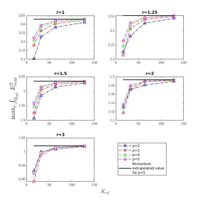
Figure 3: Asymptotic convergence of time-averaged $\int_{\Omega_{cyl}}\left(E_{z}^{s}\right)^{2}$ vs. no. of elements $K_{cyl}$ on the surface of the scattering cylinder.

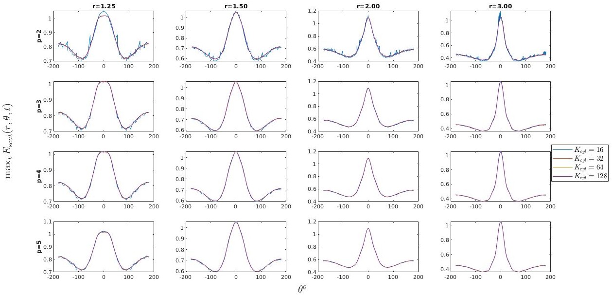
Figure 4: Asymptotic convergence of time-averaged, local $\max_{t}E_{z}^{s}$ vs. viewing angle $\theta$.

4 Divergence error based adaptivity

In this section, we summarize a re-interpretation of a known numerical error arising when solving the time-domain Maxwell’s equations, the divergence error, as an error indicator presented by us earlier in ref. [41]. Numerical solutions of the time-domain Maxwell’s equations, when obtained with methods other than the finite-difference time-domain (FDTD) methods, consist of a numerical divergence error originating from the treatment of the constraint on divergence posed by the Gauss laws. Due to the act of discretization with spatial operators having finite accuracy, the solenoidal condition on the fields is not met exactly. This results in the evolution of divergence in an initially solenoidal field, which in the continuous system is zero (in absence of sources), giving rise to numerical divergence error. There is abundant literature on the subject of divergence cleaning techniques and Gauss’ constraint satisfying methods [51, 52, 53, 54, 55, 56]. But these are only used when the underlying physics requires exactly meeting the divergence constraint, for example in magnetohydrodynamics. Apart from this exception, divergence errors accruing in conservative higher-order formulations do not significantly impact the overall accuracy of the solution [55, 57] and so, are often disregarded in practice. In [57], Cioni et. al used a mixed finite volume/finite element method to show that divergence error, despite being linked to the accuracy of the solver and the underlying discretization, does not hamper the formal accuracy of the solution.

Consider a subsystem of eq. 1 with the $TM_{z}$ mode given by eq. 2, consisting of only in-plane components $B_{x}$ and $B_{y}$, such that

$$\mathbf{U}=\begin{pmatrix}B_{x}\\ B_{y}\end{pmatrix}=\mathbf{B},\hskip 8.5359pt\mathbf{F}=\begin{pmatrix}0\\ -D_{z}/\epsilon\end{pmatrix}\hat{i},\hskip 8.5359pt\mathbf{G}=\begin{pmatrix}D_{z}/\epsilon\\ 0\end{pmatrix}\hat{j},\hskip 8.5359pt$$ (11)

with $\mathbf{S}=0$ for simplicity, and $\hat{i},\hat{j}$ being unit vectors along the $+x$ and $+y$ directions respectively. Conservation form for this subsystem came then be written in Cartesian co-ordinates as,

$$\frac{\partial\mathbf{U}}{\partial t}+\nabla\cdot\mathcal{F}=\frac{\partial\mathbf{U}}{\partial t}+\frac{\partial\mathbf{F}}{\partial x}+\frac{\partial\mathbf{G}}{\partial y}=0,$$ (12)

where the flux is given as

$$\mathcal{F}=[\mathbf{F},\mathbf{G}].$$

Writing the vector equation eq. 12 component-wise,

$$\frac{\partial}{\partial t}\begin{pmatrix}B_{x}\\ B_{y}\end{pmatrix}+\frac{\partial}{\partial x}\begin{pmatrix}0\\ -D_{z}/\epsilon\end{pmatrix}+\frac{\partial}{\partial y}\begin{pmatrix}D_{z}/\epsilon\\ 0\end{pmatrix}=0.$$ (13)

$$\frac{\partial}{\partial t}\begin{pmatrix}B_{x}\\ B_{y}\end{pmatrix}+\begin{pmatrix}\frac{\partial D_{z}/\epsilon}{\partial y}\\ \\ -\frac{\partial D_{z}/\epsilon}{\partial x}\end{pmatrix}=0.$$ (14)

A representation of eq. 14 as a time-dependent PDE, is given by

$$\frac{\partial\mathbf{U}}{\partial t}=\mathbf{R}\left(\mathbf{U}\right),$$ (15)

where $\mathbf{R}$ is the spatial operator. Consider a higher order discretization of eq. 12 of the form [5],

$$\int_{\Omega}\nabla\cdot\mathcal{F}\left(\mathbf{U}\right)\psi d\mathbf{x}=0\rightarrow\sum_{\mathbb{D}^{k}\in\Omega_{h}}\mathbf{R}_{p}\left(\mathbf{U}_{p}\right)=0,$$ (16)

where $\psi$ is a test function and $p$ is the degree of the polynomial bases used to represent the discrete solution $\mathbf{U}_{p}$. $\mathbf{R}_{p}$ represents the discrete spatial partial differential operator. A lower $q$th order approximation on the same mesh can be formed by projecting the $p$-th order accurate solution to a space of $q$-th order basis functions,

$$\tilde{\mathbf{U}}_{p}^{q}=I_{p}^{q}\mathbf{U}_{p},$$ (17)

where $I_{p}^{q}$ is the transfer operator with $p>q$, and $\left(\tilde{\cdot}\right)$ is a restricted higher order (here, $p$-th order) quantity.

A relative truncation error [17, 58] between levels $p$ and $q$, is usually defined as,

$$\bm{\tau}_{p}^{q}=I_{p}^{q}\mathbf{R}_{p}\left(\mathbf{U}_{p}\right)-\mathbf{R}_{q}\left(I_{p}^{q}\mathbf{U}_{p}\right)=\llbracket\mathbf{R}\left(\mathbf{U}\right)\rrbracket_{p}^{q}.$$ (18)

Here, the notation $\llbracket\left(\cdot\right)\rrbracket_{p}^{q}$ represents the difference between quantities at refinement levels $p$ and $q$ as shown. Operator $\mathbf{R}$ of varying spatial accuracies acts on pure and restricted solution vectors $\mathbf{U}$, via the transfer operator $I_{p}^{q}$ restricting the higher ($p$-th) order solution to a lower ($q$-th) order. This relative truncation error is commonly used in multigrid and multilevel techniques for explicit time marching schemes [59], as a forcing function for maintaining higher ($p$-th) order solution while operating at a lower ($q$-th) order. Similarly, a relative divergence error [41] is defined as

$$\gamma_{p}^{q}=\bm{\nabla}\cdot\tilde{\mathbf{B}}_{p}^{q}-\bm{\nabla}\cdot\mathbf{B}_{q}$$ (19)

The relative truncation and relative divergence errors are related to each other via the Divergence Error Evolution Equation (DEEE), which in continuous form is derived in [41] to be,

$$\boxed{\frac{d\gamma_{p}^{q}}{dt}=\bm{\nabla}\cdot\bm{\tau}_{p}^{q}}.$$ (20)

Eq. 20 expresses compactly that the relative truncation error acts as a source for the relative divergence error. For $p\rightarrow\infty$, i.e. corresponding to the continuous case, then eq. 20 suggests that it is due to the act of discretization that a divergence error is generated. The divergence error is contained in the discrete solution, and is not a result of the finite accuracy of the divergence operators used. This is emphasized above by defining $\gamma_{p}^{q}$ using infinitely accurate divergence operators.

Consider a plane wave solution to eq. 2, restricted to a single frequency $\omega$ here, as a representative instance [42],

$$D_{z}=D_{z0}e^{(\mathbf{k}\cdot\bm{x}-\omega t)},$$ (21a)

$$B_{y}=-\sqrt{\frac{\mu}{\epsilon}}D_{z}cos\phi,$$ (21b)

$$B_{x}=\sqrt{\frac{\mu}{\epsilon}}D_{z}sin\phi,$$ (21c)

where $\bm{x}$ is a position vector in the $xy$ plane; $\mathbf{k}=\frac{\omega}{c}\left[\cos\phi,\sin\phi\right]^{T}$ is the wavenumber with $\phi$ being the angle made with the $+x$ axis. $c=\frac{1}{\sqrt{\mu\epsilon}}$ is the speed of propagation in the medium. In this case, $\bm{\tau}_{p}^{q}$ defined as eq. 18 evaluates to,

$$\bm{\tau}_{p}^{q}=\llbracket\mathbf{R}\left(\mathbf{U}\right)\rrbracket_{p}^{q}=\begin{pmatrix}\left\llbracket\frac{\partial{B_{y}}}{\partial y}\right\rrbracket_{p}^{q}\frac{c}{cos\phi}\\ \\ \left\llbracket\frac{\partial B_{x}}{\partial x}\right\rrbracket_{p}^{q}\frac{c}{sin\phi}\end{pmatrix}=\begin{pmatrix}-\left\llbracket\frac{\partial{E_{z}}}{\partial y}\right\rrbracket_{p}^{q}\\ \\ \left\llbracket\frac{\partial E_{z}}{\partial x}\right\rrbracket_{p}^{q}\end{pmatrix}.$$ (22)

A relevant simplification for such a monochromatic plane wave solution using a fully discrete relative divergence error $\hat{\gamma}_{p}^{q}$ is given in [41] by,

$$\boxed{\hat{\gamma}_{p}^{q}=\bm{\tau}_{p}^{q}\cdot\frac{\bm{\phi}}{c}},$$ (23)

where $\bm{\phi}=\left[\cos\phi,\sin\phi\right]^{T}$, is a unit vector along the direction of wave travel. The fully discrete relative divergence error $\hat{\gamma}_{p}^{q}$ is defined as,

$$\hat{\gamma}_{p}^{q}=I_{p}^{q}\bm{\nabla}_{p}\cdot\mathbf{B}_{p}-\bm{\nabla}_{q}\cdot\left(I_{p}^{q}\mathbf{B}_{p}\right)=\llbracket\bm{\nabla}\cdot\mathbf{B}\rrbracket_{p}^{q},$$ (24)

which uses discrete divergence operators and includes the errors associated with them. The definition eq. 24 is a practically computable relative divergence error defined as eq. 18 [41]. $\hat{\gamma}_{p}^{q}$ is given component-wise by,

$$\hat{\gamma}_{p}^{q}=\llbracket\bm{\nabla}\cdot\mathbf{B}\rrbracket_{p}^{q}=\left\llbracket\frac{\partial B_{x}}{\partial x}\right\rrbracket_{p}^{q}+\left\llbracket\frac{\partial{B_{y}}}{\partial y}\right\rrbracket_{p}^{q}.$$ (25)

Relation 23 forms the essential link between the two errors and institutes $\hat{\gamma}$ as a scalar proxy of $\bm{\tau}$. Since the divergence error of the solution is readily available, it serves as an inexpensive driver in adaptive algorithms having the typical ease of computation of feature-based methods. However, these mutual relations make this indicator, also a rigourous truncation error-based indicator. The truncation and discretization errors are mutually related through the Discretization Error Transport Equation (DETE), which shows that truncation error acts as a local source of discretization error [5]. This made the case for preferring truncation error as a sensor in a number of adaptive algorithms for hyperbolic problems in literature. Hence, the extensive work in the area of truncation error estimation [17, 5, 6].

4.1 Comparison between local gradient and divergence errors

In section 3.3, we established EM energy as a feature-based adaptivity driver, heuristically adapting based on $\nabla E$ (subscript $z$ dropped, considering the $TM_{z}$ mode). Here, we use error in gradient of local field to potentially develop a non-heuristic, error-driven indicator, similar to the use of error in SED in solid mechanics, shown in eq. 5. For comparison with $\gamma_{p}^{q}$, consider a relative gradient error in local field $E$,

$$\bm{\nabla}\tilde{E}_{p}^{q}-\bm{\nabla}E_{q}=\llbracket\bm{\nabla}E\rrbracket_{p}^{q}=\begin{pmatrix}\left\llbracket\frac{\partial E}{\partial x}\right\rrbracket_{p}^{q}\\ \\ \left\llbracket\frac{\partial E}{\partial y}\right\rrbracket_{p}^{q}\end{pmatrix}.$$ (26)

In this context, both gradient and divergence of the solution are smoothness indicators, made of a combination of first spatial derivatives of the solution, as shown in eqns. 25 and 26. Despite this similarity, derivatives taken in the combination of divergence has an advantage over a simple gradient in the present context. From eqns. 22 and 26, it can be seen that despite the magnitudes of the relative truncation and relative gradient errors being equal, a causal relation like the one with the relative divergence error in eq. 23 does not follow.

More importantly, to compute the relative gradient error between two discretization levels, no reference value for $\nabla\tilde{E}_{p}^{q}$ is readily available limiting the use of gradient of the local field to a heuristic indicator as shown in sec. 3.3. In solid mechanics, this problem of finding a reference value for SED $\Psi^{*}$ (refer eq. 5) is overcome by estimating it, using the SED $\tilde{\Psi}$, obtained from a discrete solution followed with projection techniques. The practice of adopting an enhanced or smoothed field as a true field on the basis of the obtained numerical solution, is well established in solid mechanics [13, 33, 60, 61]. Unlike in solid mechanics, the solenoidal constraint in the time-domain Maxwell’s equations means that a known datum (of zero divergence) is available at all points in space and time. Eq. 20 establishes relative divergence error as a proxy to the relative truncation error and, the condition of null divergence makes the divergence corresponding to any single discretization level, a relative divergence error.

Therefore, unlike the relative gradient error, a divergence error based sensor need not rely on expensive estimation procedures and can be accurately computed. Moreover, it leads to a non-heuristic method eliminating the subjectivity involved with gradient-driven adaptation schemes. The divergence error-based indicator utilizes the structure of the governing equations eliminating the need to estimate reference states. It shows all desirable properties of adaptivity indicators identified in sec. 3.1, along with the added advantage of a known reference.

As pointed out earlier in the introduction, the high cost of computation of an error indicator, and accommodating tedious computations in an existing code structure are limiting factors for the practical use of adaptive algorithms in commerical software [62]. Since computing divergence only uses derivatives of the solution vector, requisite routines are usually already available in an existing code, making it practically feasible to incorporate such an indicator. It is co-ordinate independent and a scalar, and combines the rigour of truncation error driven methods, with the practicality of feature-driven methods.

The effort to advance from heuristic feature-driven methods to fully automated, rigorous error-driven adaptive methods seen in solid mechanics, is made here for the time-domain Maxwell’s equations. We construct an adaptation routine based on the gradient of EM energy, followed by another, utilizing a divergence error indicator.

The arguments presented thus far, are summarized as follows:

1. Like gradient of SED in solid mechanics, gradient of EM energy has been used for the time-domain Maxwell’s equations, both leading to heuristic, feature-based adaptive schemes.

2. To advance from a heuristic feature driven method to an automated error-driven adaptive method, error in SED is used as an estimate of the discretization error in solid mechanics. With the hyperbolic time-domain Maxwell’s equations, use of gradient of EM energy is limited to a feature-based method since it neither shows a direct relation with the relative truncation error, nor is economically computable.

3. A re-interpretation of the divergence error, inherent to any (except FDTD and dedicated divergence-free methods) numerical solution of the time-domain Maxwell’s equations, establishes it as a proxy to the relative truncation error.

4. Along with having all desirable properties identified from the well-established SED-based indicators in solid mechanics, the divergence error has an additional advantage of being exactly computable, eliminating typical estimation procedures.

5 Results

We present results for 3 testcases in this section - scattering from a PEC circular cylinder, a semi-open cavity, and a case of two adjacent PEC circular cylinders. These problems represent complexities arising from scatterers with various geometries and configurations. Uniform $p$ solutions are compared to the adaptive $p$ solutions for accuracy, along with a comparison of computational performance between the two adaptivity drivers: one based on gradient of the local field, and the other on divergence error of the solution. For a fair comparison, both adaptive methods use the same algorithm with respective local indicators as input to map them to a $p$-distribution. The algorithm takes a logarithm of the local data, segregating it into different orders of magnitude, and maps the highest value to a preset maximum allowable $p$, which is taken to be $8$, and the lowest to $1$ with all intermediate values mapped linearly. Hence, every node gets mapped to a proposed $p$ for the next iteration and the maximum $p$ amongst all nodes within an element is chosen. The elements forming the PML layer to truncate the domain boundaries, are manitained at the highest, i.e. $8$-th order to resolve the rapidly decaying fields. For a thorough description, we refer the reader to [41].

In EM wave scattering problems, a scattered wave is formed at the PEC boundary and propagated away from it. Thus, the scatterer acts as a local source resulting in a relatively higher divergence error close to its boundaries. Also, as the wave progresses in space, similar behaviour is expected along the foremost, or leading wavefront. Hence, we expect the divergence-driven adaptive method to allocate denser close to the scattering surface and the leading wavefront. Likewise, the higher relative gradients close to the scattering body due to its being the source, is expected to cause the gradient-based adaptive method to allocate denser. Additionally, unlike divergence, the harmonic scattered wave advecting in space, is expected to have higher relative gradients in the region between the scatterer and the leading wavefront as well, especially in the shadow region, as is typical in scattering problems. Hence, the distribution of $p$ across elements obtained using the gradient-driven adaptive method, is expected to qualitatively follow the contour of the local field, refining (by raising local $p$) along the boundary of the scatterer and extending it upto the leading wavefront.

5.1 Scattering off a circular cylinder

Figure 6: Schematic for the circular cylinder scattering problem

The two proposed drivers are applied to the problem of scattering from a PEC cylinder for validation. A schematic of the problem is shown in fig. 6. Variations of the problem in terms of electrical sizes and incident TM and TE illumination are presented.

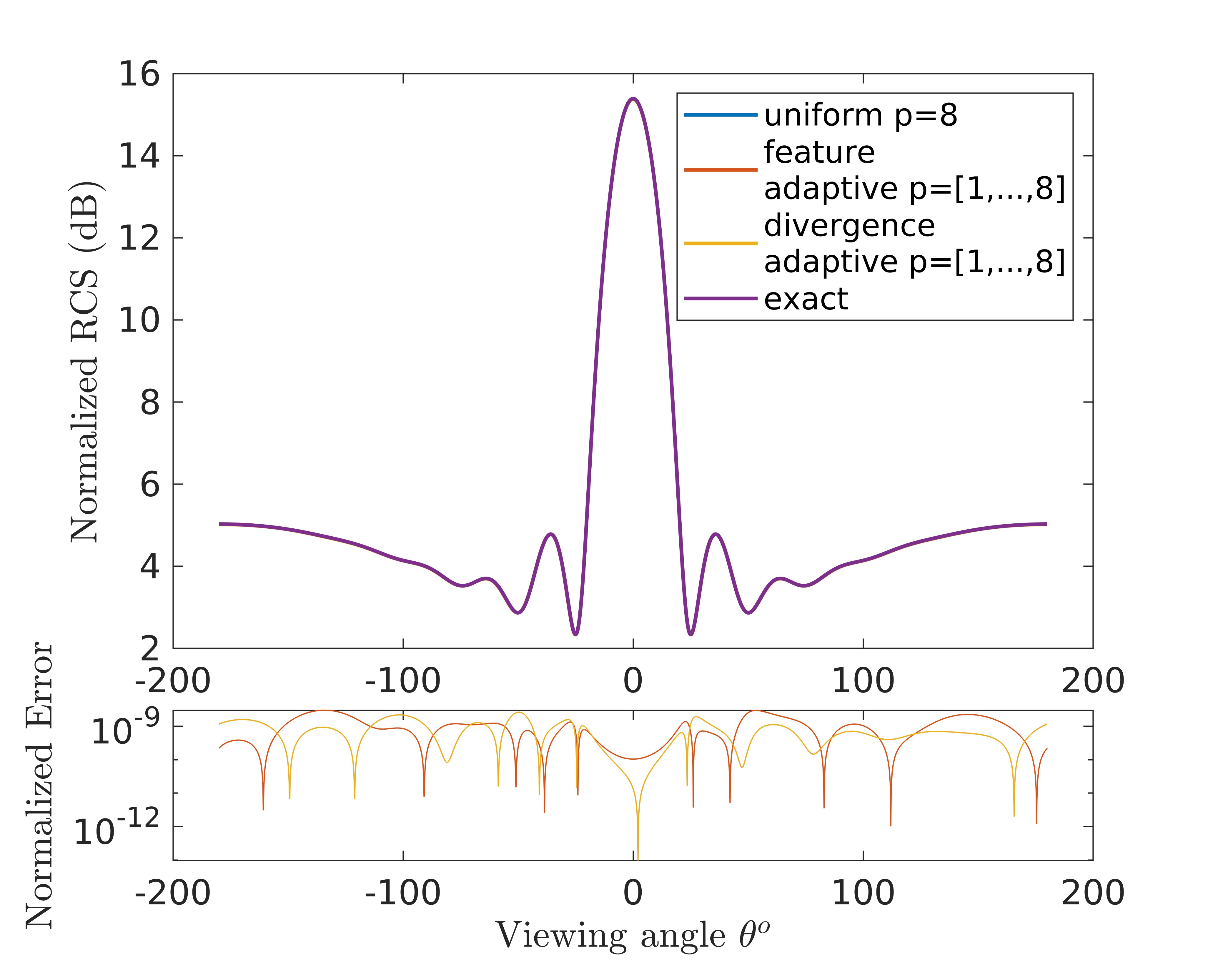
Figure 7: RCS, circular cylinder scattering, size $2\lambda$, TM illumination

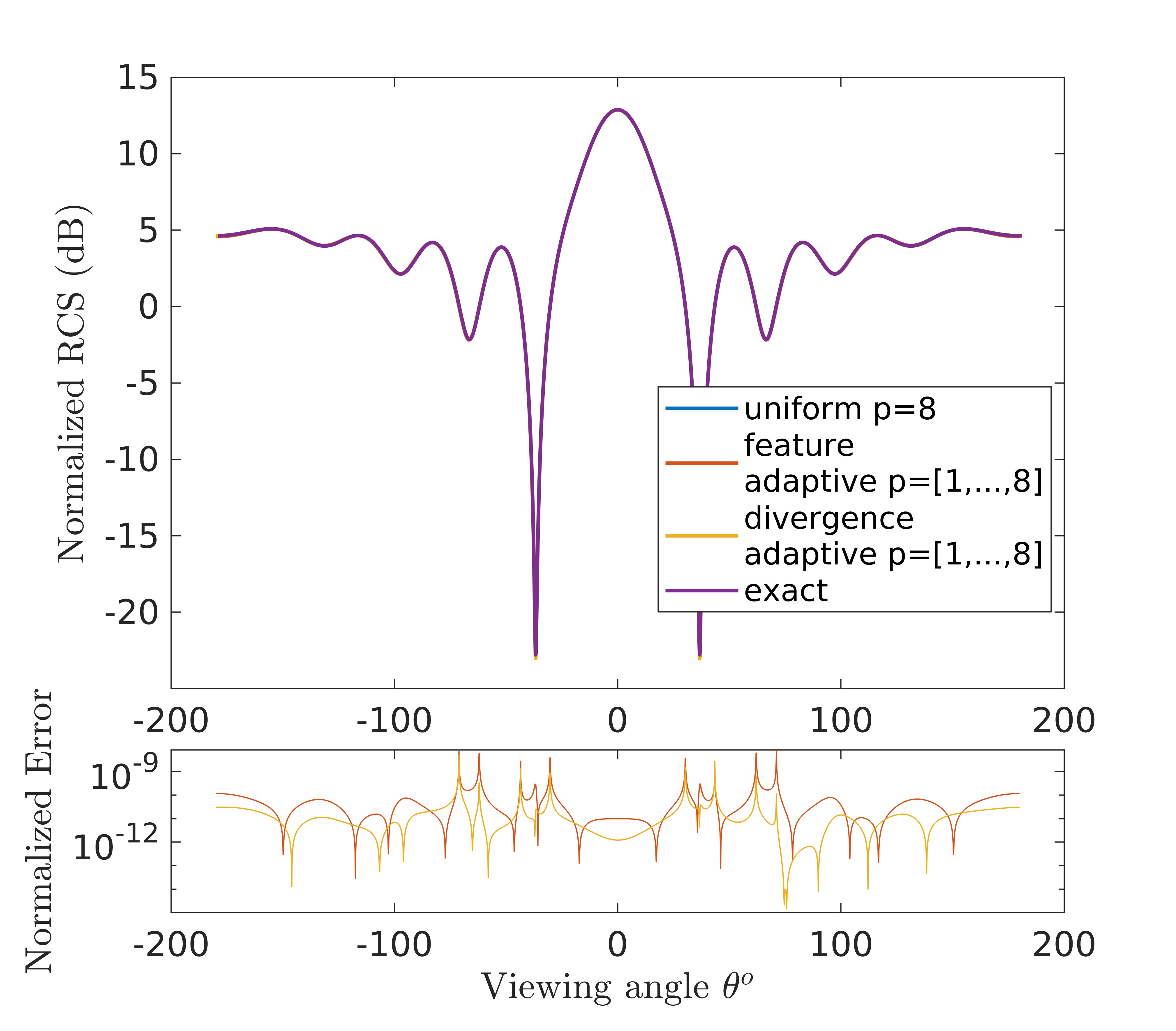
Figure 8: RCS, circular cylinder scattering, size $2\lambda$, TE illumination

The scattering width obtained numerically, compared to the exact solutions are shown in figs. 7 and 8, under TM and TE illuminations respectively, for a scatterer $2\lambda$ in diameter. Fig. 9 shows another instance with a larger scatterer, $15\lambda$ in size. 4 lines plots overlay each other including a uniform order method to compare against the 2 adaptive methods. For this canonical case, the exact solution is known and is plotted for comparison. Since the plots are visually indistinguishable, the difference between the RCS obtained using the adaptive $p=[1,\cdots,N]$ and uniform $p=N$ solutions is also shown. Viewing angle $\theta$ referred to in these plots, is measured from the $+x$ axis as depicted in the schematic fig. 6. The adaptation routine operates after every iteration throughout the duration of the problem, including an initial unsteady phase, evolving into a harmonically steady state.

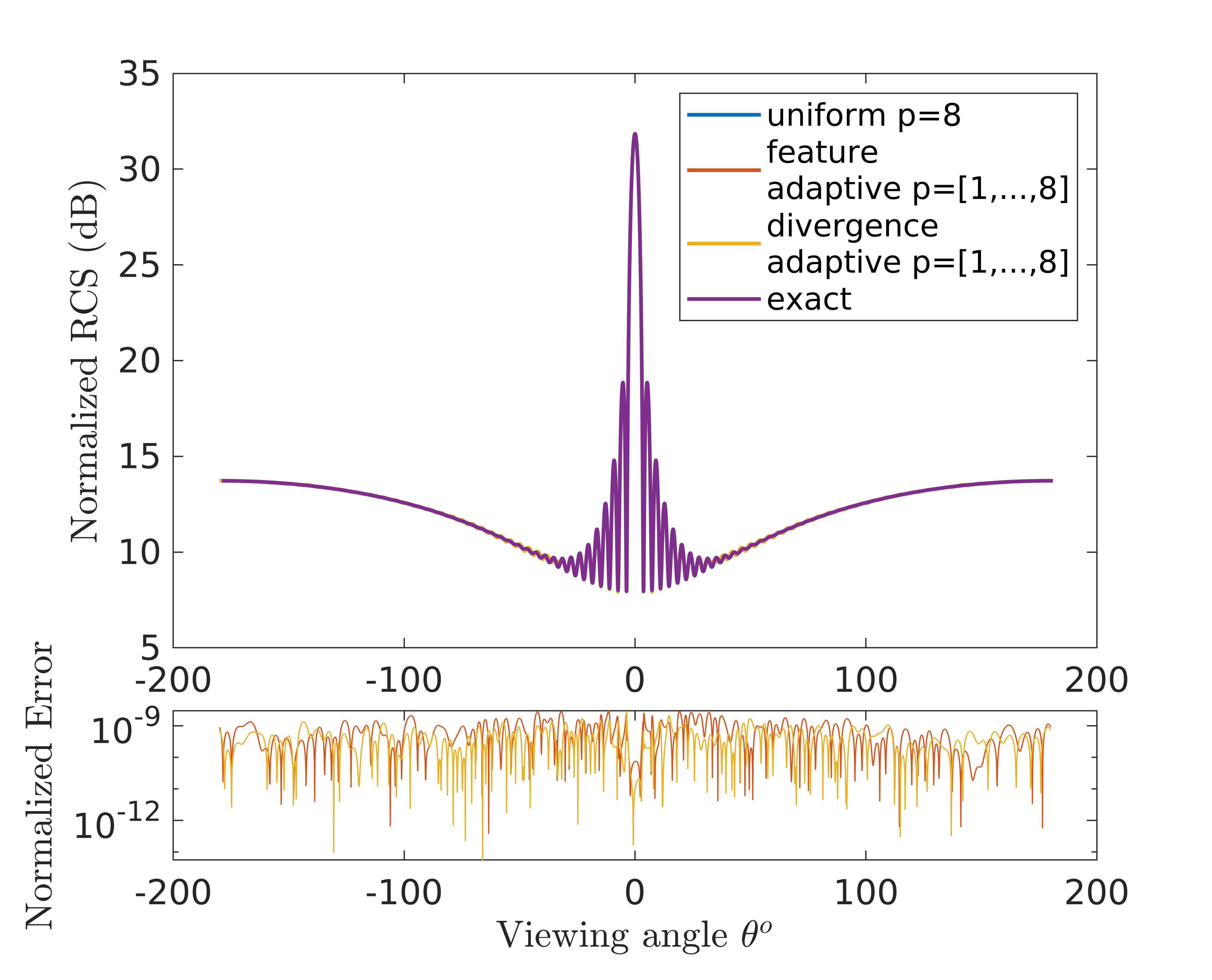
Figure 9: RCS, circular cylinder scattering, size $15\lambda$, TM illumination

To demonstrate the dynamic behaviour of the two adaptation criteria, fig. LABEL:fig:pdis1cyl shows the scattered $E_{z}$ at the 4 time-period mark and the corresponding distributions of $p$ resulting from the adaptation. The divergence-based identifies local sources of divergence at the scattering surface, and along the leading wavefront travelling away from the body. This becomes significant in case of mutually interacting waves from multiple scattering surfaces, presented in later sections. Unlike divergence, the gradients do not decay away from the scatterer resulting in the feature-based method allocating higher order elements more densely as compared to that of the divergence error based driver since the gradients do not localize based strictly on the truncation error. The $p$-distribution pattern follows the contour of $E_{z}$ instead.

5.2 Semi-open cavity

Figure 11: Schematic for the semi-open cavity problem

Fig. 11 shows a schematic of the semi-open cavity problem. A TE monochromatic plane wave travels towards the closed-end of the cavity. The computational domain includes a PML 1$\lambda$ wide at the outer boundaries to truncate the domain. 12. The overlaid RCS plots in fig. 12 show that the adaptive solutions are essentially as accurate as the uniform $p$ solution. A $5$th order accurate hybrid Galerkin solution to this problem, presented in [63] has been used as reference. Results shown have been computed at the 40 period mark, the solution being well converged.

Figure 12: RCS, semi-open cavity problem.

We compare the $p$-distributions at an intermediate time level of 4 periods in the unsteady regime to highlight key differences between the two adaptation schemes, in fig. LABEL:fig:pdisSOcavity. The scattered wave in the cavity has reached halfway length and this raises the local divergence near this region, as also at the corners, seen in the divergence-based $p$-distribution. The contours of $H_{z}$ also show that the scattered waves emerging at both open and closed ends of the cavity (along $x$-axis) completely surround the scattering surface. This creates higher relative gradients around the scattering surface resulting in denser allocation by the feature-based method, compared to the divergence error based, that localizes most higher order elements along the scattering surfaces.

5.3 Two adjacent cylinders

Figure 14: Schematic for the scattering off 2 adjacent cylinders problem

Another canonical problem that addresses the complexity of multiple reflections and reciprocal interactions is that of multiple scatterers [64]. Here, we investigate scattering from two adjacent circular cylindrical PEC scatterers, the schematic for which is shown in fig. 14. An incident TE wave illuminates the two cylinders travelling along the $-y$ axis. The distance separating the scatterers ($6.4$ wavelengths) and the diameter of each ($4$ wavelengths) makes it lie in the optical scattering range. The circular domain is truncated with a PML $1\lambda$ wide with the interface located at a radius of 7.5, and the outermost boundary at radius 8.5. The solution takes 50 periods to converge and a reference RCS plot is taken from [63] that used a $6$th order accurate hybrid Galerkin solution.

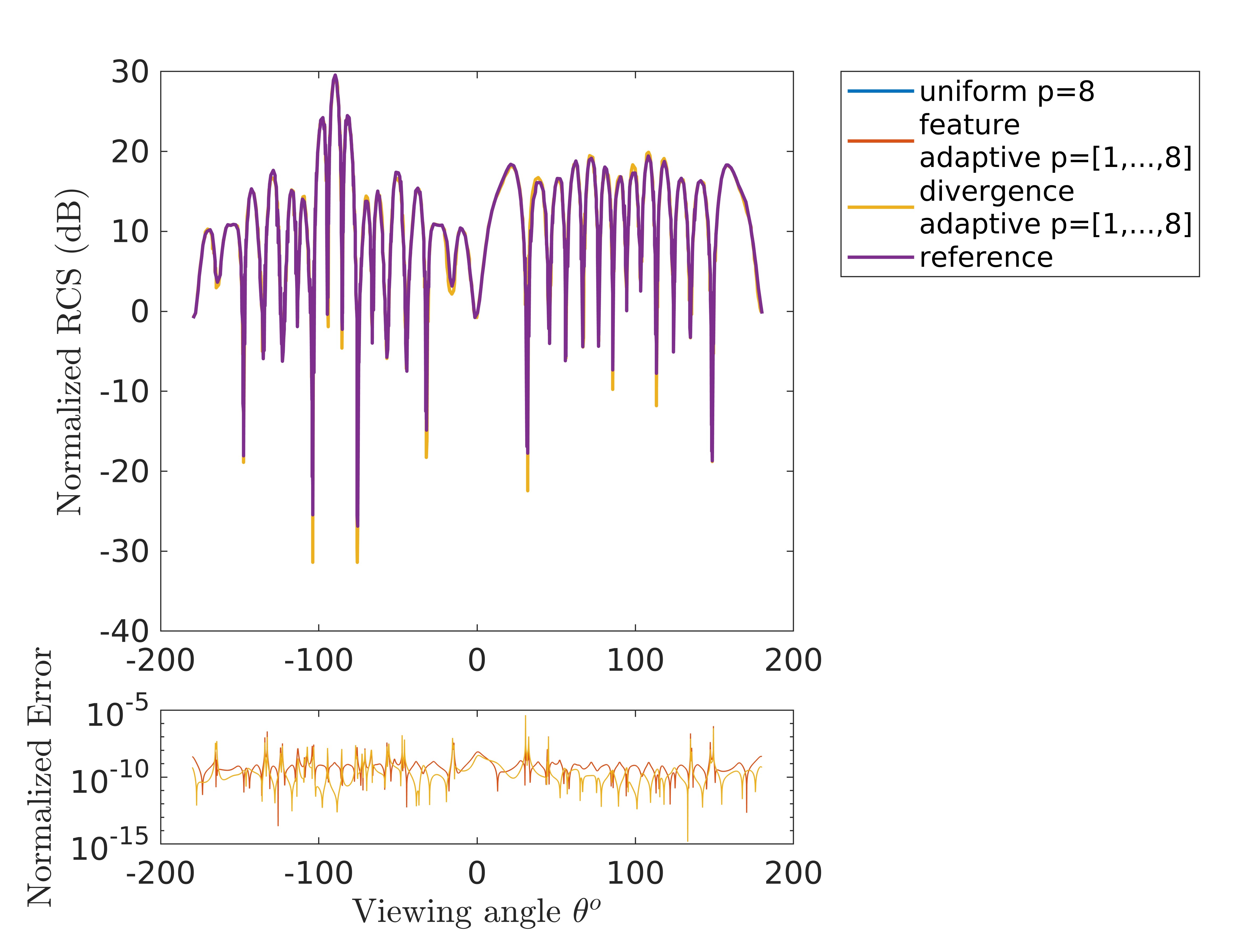
Figure 15: RCS, 2 adjacent cylinders problem

Continuing with the pattern of presenting RCS results as in earlier sections, fig. 15 shows the uniform, adaptive and reference plots. The uniform and the adaptive solution plots are close to each other and in agreement with the reference.

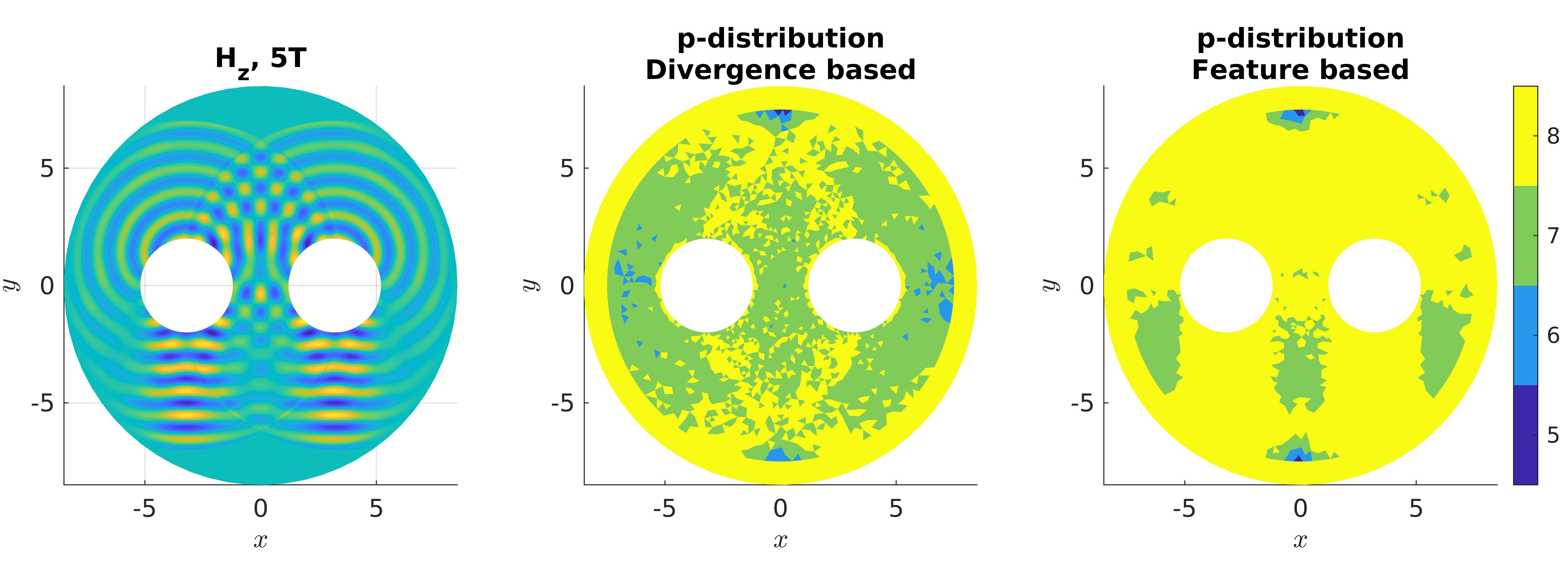
Figure 16: Comparison between $p$ distributions, 2 adjacent cylinders problem

Fig. 16 compares $p$-distributions at the 5 period mark, developed enough to show all key features. The contour on the lit side (the upper half) shows two leading wavefronts scattered off each cylinder, and also off the neighbouring cylinder. The divergence error driver captures these wavefronts in both the illuminated and shadow regions. The gradient-driven method on the other hand, follows the contours of the scattered field closely, along with a characteristic denser allocation as seen in previous cases.

For similar accuracies (determined by the resulting RCS from both methods), it is observed that the divergence error based method leads to a more economical allocation of $p$, concentrating the DOFs to local sources of divergence error, and in turn truncation errors. The scattering surface acting as a local source of divergence error, gets assigned a denser allocation of higher order elements relative to the region between the surface and the leading wavefront. Also, the divergence-error based method tracks the leading wavefront of the scattered wave from a body on its way to a neighbouring scatterer, thereby maintaining higher order accuracy in cases of mutually interacting waves between multiple scatterers. On the other hand, a feature-based method driven by gradient of the local field, allocates denser not only close to the scattering surface, but also in the region upto the leading wavefront following the harmonic scattered wave. Hence, unlike divergence error, it results in over-compensating by concentrating DOFs closer to, but also away from local truncation error sources. This leads to a higher demand in DOFs, quantified in the following section.

5.4 Computational performance

Problem	Savings in DOFs (%)		effective $p$
	Divergence error	Gradient of energy	Divergence error	Gradient of energy
1 cylinder, 2$\lambda$, TM	43.14	31.36	5.31	6.07
1 cylinder, 2$\lambda$, TE	43.41	31.34	5.30	6.07
1 cylinder, 15$\lambda$, TM	34.36	20.86	5.90	6.72
1 cylinder, 15$\lambda$, TE	35.01	20.84	5.87	6.73
Semi-open cavity	25.95	18.12	6.31	6.82
2 adjacent cylinders	23.39	13.77	6.57	7.23

Table 1: Computational savings in DOFs and effective $p$ employed to achieve accuracy corresponding to a uniform 8th order method.

In this section, we compare the computational gain from the two proposed adaptive methods. For equally accurate solutions, the two schemes evolve different $p$-distributions and the impact on computational savings is compared in table 1. The savings in DOFs are compared to a uniform $p$ solution. The effective $p$ shown for individual testcases, is the $p$, averaged over time and space. It serves as a measure of the computational savings made in obtaining $8$-th order accurate solutions with methods using lower order spatial operators, in an average sense. While considerable savings are made in all testcases, the recurring theme of the feature-based scheme using denser allocations than the divergence error-based, follows from the $p$-distribution plots shown in earlier sections, and is quantified in table 1.

6 Conclusion

An extension of the principles on which established drivers for adaptive methods in solid mechanics are based upon, is made to CEM for non-FDTD solutions to the time-domain Maxwell’s equations. A feature-based method guided by gradient of local EM energy, and another using the divergence error are presented. The proposed methods use a combination of spatial operators locally varying in order of accuracy, to achieve higher order accurate solutions, using fewer degrees of freedom. Numerical results for canonical testcases of scattering problems are presented demonstrating the effectiveness of the proposed schemes. Theoretically, it is shown that the role strain energy plays in adaptive methods for solid mechanics of acting as a proxy to numerical error, EM energy in the current context cannot. Unlike strain energy, EM energy does not contain any more information than the solution and despite showing some desirable properties, is not a viable substitute. The use of EM energy as an adaptivity driver remains limited to only a heuristic, feature-based method. As an alternative, the relation between truncation and divergence errors is used to develop a divergence error driven adaptive algorithm. The highlight of using the proposed divergence error driver is that it needs no expensive error estimation algorithms and is easily computed. This is enabled by the knowledge of a reference state of null divergence, afforded in the time-domain Maxwell’s equations, a distinguishing feature from other applications. Divergence error makes for a robust indicator to develop automated, error-driven adaptive methods. The divergence error indicator not only satisfies all requisite properties that established error indicators in solid mechanics possess, it is easily incorporated in existing code structures. More importantly, it is highlighted that numerical divergence error when not detrimental to the underlying physics, may be utilized to a computational gain.

References

- [1] I Babuška “The p and h-p Versions of the Finite Element Method: The State of the Art” In Finite Elements New York, NY: Springer New York, 1988, pp. 199–239 DOI: 10.1007/978-1-4612-3786-0˙10
- [2] I. Babuska “The p-version of the finite element method” In SIAM Journal on Numerical Analysis 18.3, 1981
- [3] I. Babuška and W. Gui “Basic principles of feedback and adaptive approaches in the finite element method” In Computer Methods in Applied Mechanics and Engineering 55.1-2, 1986, pp. 27–42 DOI: 10.1016/0045-7825(86)90084-8
- [4] Moritz Kompenhans, Gonzalo Rubio, Esteban Ferrer and Eusebio Valero “Adaptation strategies for high order discontinuous Galerkin methods based on Tau-estimation” In Journal of Computational Physics 306.December Elsevier Inc., 2016, pp. 216–236 DOI: 10.1016/j.jcp.2015.11.032
- [5] Moritz Kompenhans, Gonzalo Rubio, Esteban Ferrer and Eusebio Valero “Comparisons of p-adaptation strategies based on truncation- and discretisation-errors for high order discontinuous Galerkin methods” In Computers & Fluids 139 Elsevier Ltd, 2016, pp. 36–46 DOI: 10.1016/j.compfluid.2016.03.026
- [6] Alexandros Syrakos, Georgios Efthimiou, John G. Bartzis and Apostolos Goulas “Numerical experiments on the efficiency of local grid refinement based on truncation error estimates” In Journal of Computational Physics 231.20 Elsevier Inc., 2012, pp. 6725–6753 DOI: 10.1016/j.jcp.2012.06.023
- [7] Li Wang and Dimitri J. Mavriplis “Adjoint-based h-p adaptive discontinuous Galerkin methods for the 2D compressible Euler equations” In Journal of Computational Physics 228.20 Elsevier Inc., 2009, pp. 7643–7661 DOI: 10.1016/j.jcp.2009.07.012
- [8] Niles A. Pierce and Michael B. Giles “Adjoint and defect error bounding and correction for functional estimates” In Journal of Computational Physics 200.2, 2004, pp. 769–794 DOI: 10.1016/j.jcp.2004.05.001
- [9] David A. Venditti and David L. Darmofal “Grid adaptation for functional outputs: Application to two-dimensional inviscid flows” In Journal of Computational Physics 176.1, 2002, pp. 40–69 DOI: 10.1006/jcph.2001.6967
- [10] Ralf Hartmann and Paul Houston “Adaptive discontinuous Galerkin finite element methods for the compressible Euler equations” In Journal of Computational Physics 183.2, 2002, pp. 508–532 DOI: 10.1006/jcph.2002.7206
- [11] M. J. Aftosmis “Upwind method for simulation of viscous flow on adaptively refined meshes” In AIAA Journal 32.2, 1994, pp. 268–277 DOI: 10.2514/3.11981
- [12] Jean François Remacle, Joseph E. Flaherty and Mark S. Shephard “An adaptive discontinuous Galerkin technique with an orthogonal basis applied to compressible flow problems” In SIAM Review 45.1, 2003, pp. 53–72 DOI: 10.1137/S00361445023830
- [13] A. Hernández, J. Albizuri, M.B.G. Ajuria and M.V. Hormaza “An adaptive meshing automatic scheme based on the strain energy density function” In Engineering Computations 14.6, 1997, pp. 604–629 DOI: 10.1108/02644409710367476
- [14] Yunhua Luo and Ulrich Häussler-Combe “A gradient-based adaptation procedure and its implementation in the element-free Galerkin method” In International Journal for Numerical Methods in Engineering 56.9, 2003, pp. 1335–1354 DOI: 10.1002/nme.615
- [15] Fabio Naddei, Marta. de la Llave Plata and Vincent Couaillier “A comparison of refinement indicators for p-adaptive discontinuous Galerkin methods for the Euler and Navier-Stokes equations” In 2018 AIAA Aerospace Sciences Meeting Reston, Virginia: American Institute of AeronauticsAstronautics, 2018, pp. 0368 DOI: 10.2514/6.2018-0368
- [16] François Fraysse, Eusebio Valero and Jorge Ponsín “Comparison of mesh adaptation using the adjoint methodology and truncation error estimates” In AIAA Journal 50.9, 2012, pp. 1920–1932 DOI: 10.2514/1.J051450
- [17] Andrés M. Rueda-Ramírez, Gonzalo Rubio, Esteban Ferrer and Eusebio Valero “Truncation Error Estimation in the p-Anisotropic Discontinuous Galerkin Spectral Element Method” In Journal of Scientific Computing 78.1 Springer US, 2019, pp. 433–466 DOI: 10.1007/s10915-018-0772-0
- [18] Thomas Grätsch and Klaus Jürgen Bathe “A posteriori error estimation techniques in practical finite element analysis” In Computers and Structures 83.4-5, 2005, pp. 235–265 DOI: 10.1016/j.compstruc.2004.08.011
- [19] Mark Ainsworth and J. Tinsley. Oden “A Posteriori Error Estimation in Finite Element Analysis” In Wiley-Interscience, 2000 DOI: 10.1016/S0045-7825(96)01107-3
- [20] Christopher Roy “Review of Discretization Error Estimators in Scientific Computing” In 48th AIAA Aerospace Sciences Meeting Including the New Horizons Forum and Aerospace Exposition, 2010, pp. 1–29 DOI: 10.2514/6.2010-126
- [21] O. C. Zienkiewicz and J Z Zhu “A simple error estimator and adaptive procedure for practical engineerng analysis” In International Journal for Numerical Methods in Engineering 24.2, 1987, pp. 337–357 DOI: 10.1002/nme.1620240206
- [22] R. J. Melosh and P. V. Marcal “An energy basis for mesh refinement of structural continua” In International Journal for Numerical Methods in Engineering 11.7, 1977, pp. 1083–1091 DOI: 10.1002/nme.1620110705
- [23] Mark S Shephard, Richard H Gallagher and John F Abel “The synthesis of near-optimum finite element meshes with interactive computer graphics” In International Journal for Numerical Methods in Engineering 15.7, 1980, pp. 1021–1039 DOI: 10.1002/nme.1620150705
- [24] M. E. Botkin “An adaptive finite element technique for plate structures” In AIAA Journal 23.5, 1985, pp. 812–814 DOI: 10.2514/3.8990
- [25] Pascal Heid, Benjamin Stamm and Thomas P. Wihler “Gradient flow finite element discretizations with energy-based adaptivity for the Gross-Pitaevskii equation” In Journal of Computational Physics 436.200021 Elsevier Inc., 2021, pp. 110165 DOI: 10.1016/j.jcp.2021.110165
- [26] Francois Henrotte and Kay Hameyer “The Energy Viewpoint in Computational Electromagnetics”, 2007, pp. 261–273 DOI: 10.1007/978-3-540-71980-9˙27
- [27] Athanasios C Antoulas, Danny C Sorensen and Serkan Gugercin “A Survey of Model Reduction Methods for Large-Scale Systems”, 2000
- [28] Su Yan et al. “A discontinuous galerkin time-domain method with dynamically adaptive cartesian mesh for computational electromagnetics” In IEEE Transactions on Antennas and Propagation 65.6 IEEE, 2017, pp. 3122–3133 DOI: 10.1109/TAP.2017.2689066
- [29] Su Yan and Jian Ming Jin “A Dynamic p-Adaptive DGTD Algorithm for Electromagnetic and Multiphysics Simulations” In IEEE Transactions on Antennas and Propagation 65.5 IEEE, 2017, pp. 2446–2459 DOI: 10.1109/TAP.2017.2676724
- [30] Luis E. Garcia-Castillo, David Pardo and Leszek F. Demkowicz “Energy-norm-based and goal-oriented automatic hp adaptivity for electromagnetics: Application to waveguide Discontinuities” In IEEE Transactions on Microwave Theory and Techniques 56.12, 2008, pp. 3039–3049 DOI: 10.1109/TMTT.2008.2007096
- [31] David Pardo, Luis E. García-Castillo, Leszek F. Demkowicz and Carlos Torres-Verdín “A two-dimensional self-adaptive hp finite element method for the characterization of waveguide discontinuities. Part II: Goal-oriented hp-adaptivity” In Computer Methods in Applied Mechanics and Engineering 196.49-52, 2007, pp. 4811–4822 DOI: 10.1016/j.cma.2007.06.023
- [32] M. Bürg “Convergence of an automatic hp-adaptive finite element strategy for Maxwell’s equations” In Applied Numerical Mathematics 72 Elsevier B.V., 2013, pp. 188–204 DOI: 10.1016/j.apnum.2013.04.008
- [33] A Tessler, H.R Riggs and S.C Macy “A variational method for finite element stress recovery and error estimation” In Computer Methods in Applied Mechanics and Engineering 111.3-4, 1994, pp. 369–382 DOI: 10.1016/0045-7825(94)90140-6
- [34] P. S. Donzelli et al. “Automated adaptive analysis of the biphasic equations for soft tissue mechanics using a posteriori error indicators” In International Journal for Numerical Methods in Engineering 34.3, 1992, pp. 1015–1033 DOI: 10.1002/nme.1620340322
- [35] Paul Houston and Endre Süli “A note on the design of hp-adaptive finite element methods for elliptic partial differential equations” In Computer Methods in Applied Mechanics and Engineering 194.2-5, 2005, pp. 229–243 DOI: 10.1016/j.cma.2004.04.009
- [36] Mark Ainsworth and Bill Senior “An adaptive refinement strategy for hp-finite element computations” In Applied Numerical Mathematics 26.1-2, 1998, pp. 165–178 DOI: 10.1016/S0168-9274(97)00083-4
- [37] T. Eibner and J. M. Melenk “An adaptive strategy for hp-FEM based on testing for analyticity” In Computational Mechanics 39.5, 2007, pp. 575–595 DOI: 10.1007/s00466-006-0107-0
- [38] V. Heuveline and R. Rannacher “Duality-based adaptivity in the hp-finite element method” In Journal of Numerical Mathematics 11.2, 2003, pp. 95–113 DOI: 10.1163/156939503766614126
- [39] W. Rachowicz, D. Pardo and L. Demkowicz “Fully automatic hp-adaptivity in three dimensions” In Computer Methods in Applied Mechanics and Engineering 195.37-40, 2006, pp. 4816–4842 DOI: 10.1016/j.cma.2005.08.022
- [40] Yunhua Luo “r-Adaptation algorithm guided by gradients of strain energy density” In International Journal for Numerical Methods in Biomedical Engineering 26.8, 2008, pp. 1077–1086 DOI: 10.1002/cnm.1209
- [41] Apurva Tiwari and Avijit Chatterjee “Divergence Error Based p-adaptive Discontinuous Galerkin Solution of Time-domain Maxwell’s Equations” In Progress In Electromagnetics Research B 96.September, 2022, pp. 153–172 DOI: 10.2528/PIERB22080403
- [42] Jan S. Hesthaven and Tim Warburton “Nodal Discontinuous Galerkin Methods” 54, Texts in Applied Mathematics New York, NY: Springer New York, 2008 DOI: 10.1007/978-0-387-72067-8
- [43] D Moxey et al. “Towards p-Adaptive Spectral/hp Element Methods for Modelling Industrial Flows” In Spectral and High Order Methods for Partial Differential Equations ICOSAHOM 2016 Cham: Springer International Publishing, 2017, pp. 63–79
- [44] Saul Abarbanel and David Gottlieb “On the construction and analysis of absorbing layers in CEM” In Applied Numerical Mathematics 27.4, 1998, pp. 331–340 DOI: 10.1016/S0168-9274(98)00018-X
- [45] M E Botkin “An adaptive finite element technique for plate structures” In AIAA Journal 23.5, 1985, pp. 812–814 DOI: 10.2514/3.8990
- [46] Peter S Donzelli et al. “Automated adaptive analysis of the biphasic equations for soft tissue mechanics using a posteriori error indicators” In International Journal for Numerical Methods in Engineering 34.3, 1992, pp. 1015–1033 DOI: 10.1002/nme.1620340322
- [47] Su Yan and Jian Ming Jin “A Dynamic p-Adaptive DGTD Algorithm for Electromagnetic and Multiphysics Simulations” In IEEE Transactions on Antennas and Propagation 65.5, 2017, pp. 2446–2459 DOI: 10.1109/TAP.2017.2676724
- [48] “Examining Spatial (Grid) Convergence” URL: https://www.grc.nasa.gov/www/wind/valid/tutorial/spatconv.html
- [49] P. J. Roache “Quantification of uncertainty in computational fluid dynamics” In Annual Review of Fluid Mechanics 29, 1997, pp. 123–160 DOI: 10.1146/annurev.fluid.29.1.123
- [50] David J. Griffiths “Introduction To Electrodynamics”, 1999
- [51] Bernardo Cockburn, Fengyan Li and Chi-Wang Shu “Locally divergence-free discontinuous Galerkin methods for the Maxwell equations” In Journal of Computational Physics 194.2, 2004, pp. 588–610 DOI: 10.1016/j.jcp.2003.09.007
- [52] Fengyan Li and Liwei Xu “Arbitrary order exactly divergence-free central discontinuous Galerkin methods for ideal MHD equations” In Journal of Computational Physics 231.6 Elsevier Inc., 2012, pp. 2655–2675 DOI: 10.1016/j.jcp.2011.12.016
- [53] Sergey Yakovlev, Liwei Xu and Fengyan Li “Locally divergence-free central discontinuous Galerkin methods for ideal MHD equations” In Journal of Computational Science 4.1-2 Elsevier B.V., 2013, pp. 80–91 DOI: 10.1016/j.jocs.2012.05.002
- [54] Praveen Chandrashekar “A Global Divergence Conforming DG Method for Hyperbolic Conservation Laws with Divergence Constraint” In Journal of Scientific Computing 79.1 Springer US, 2019, pp. 79–102 DOI: 10.1007/s10915-018-0841-4
- [55] C.-D. Munz et al. “Divergence Correction Techniques for Maxwell Solvers Based on a Hyperbolic Model” In Journal of Computational Physics 161.2, 2000, pp. 484–511 DOI: 10.1006/jcph.2000.6507
- [56] F. Assous et al. “On a Finite-Element Method for Solving the Three-Dimensional Maxwell Equations” In Journal of Computational Physics 109.2, 1993, pp. 222–237 DOI: 10.1006/jcph.1993.1214
- [57] J.P. Cioni, Loula Fezoui and Herve Steve “A Parallel Time-Domain Maxwell Solver Using Upwind Schemes and Triangular Meshes” In IMPACT of Computing in Science and Engineering 5.3, 1993, pp. 215–247 DOI: 10.1006/icse.1993.1010
- [58] F. Fraysse, J. De Vicente and E. Valero “The estimation of truncation error by -estimation revisited” In Journal of Computational Physics 231.9 Elsevier Inc., 2012, pp. 3457–3482 DOI: 10.1016/j.jcp.2011.09.031
- [59] Avijit Chatterjee “A Multilevel Numerical Approach with Application in Time-Domain Electromagnetics” In Communications in Computational Physics 17.3, 2015, pp. 703–720 DOI: 10.4208/cicp.181113.271114a
- [60] E Hinton and J S Campbell “Local and global smoothing of discontinuous finite element functions using a least squares method” In International Journal for Numerical Methods in Engineering 8.3, 1974, pp. 461–480 DOI: 10.1002/nme.1620080303
- [61] Ted Blacker and Ted Belytschko “Superconvergent patch recovery with equilibrium and conjoint interpolant enhancements” In International Journal for Numerical Methods in Engineering 37.3, 1994, pp. 517–536 DOI: 10.1002/nme.1620370309
- [62] O. C. Zienkiewicz, Robert L. Taylor and J. Z. Zhu “The Finite Element Method : Its Basis and Fundamentals” Butterworth-Heinemann, 2013
- [63] R. W. Davies, K. Morgan and O. Hassan “A high order hybrid finite element method applied to the solution of electromagnetic wave scattering problems in the time domain” In Computational Mechanics 44.3, 2009, pp. 321–331 DOI: 10.1007/s00466-009-0377-4
- [64] J. W. Young and J. C. Bertrand “Multiple scattering by two cylinders” In Journal of the Acoustical Society of America 58.6, 1975, pp. 1190–1195 DOI: 10.1121/1.380792