AsyncNeRF: Learning Large-scale Radiance Fields from Asynchronous RGB-D Sequences with Time-Pose Function

Abstract

Large-scale radiance fields are promising mapping tools for smart transportation applications like autonomous driving or drone delivery. But for large-scale scenes, compact synchronized RGB-D cameras are not applicable due to limited sensing range, and using separate RGB and depth sensors inevitably leads to unsynchronized sequences. Inspired by the recent success of self-calibrating radiance field training methods that do not require known intrinsic or extrinsic parameters, we propose the first solution that self-calibrates the mismatch between RGB and depth frames. We leverage the important domain-specific fact that RGB and depth frames are actually sampled from the same trajectory and develop a novel implicit network called the time-pose function. Combining it with a large-scale radiance field leads to an architecture that cascades two implicit representation networks. To validate its effectiveness, we construct a diverse and photorealistic dataset that covers various RGB-D mismatch scenarios. Through a comprehensive benchmarking on this dataset, we demonstrate the flexibility of our method in different scenarios and superior performance over applicable prior counterparts. Codes, data, and models will be made publicly available.

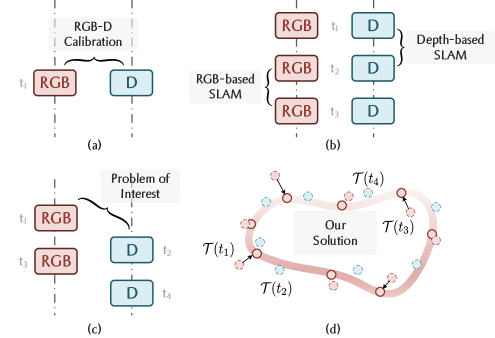
Figure 1: A conceptual demonstration of the comparison between our problem of interest and other existing problems, and our solution of learning an implicit time-pose representation.

1 Introduction

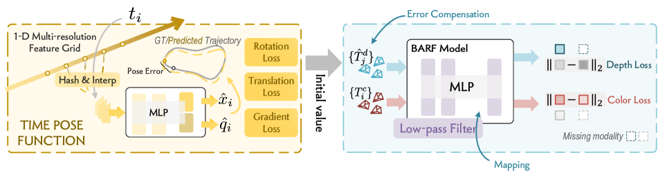
Figure 2: System Overview Our system optimization process can be divided into two stages. In the first stage, the time-pose function learns the unknown deep camera poses from an implicit functional relationship between time and camera poses in the RGB sequence. In the second stage, the complementary poses are used to train an implicit 3D scene representation with depth supervision, and the estimated poses are simultaneously refined.

Recently, Neural Radiance Fields [15] have been successfully extended to represent large-scale scenes by methods like Block-NeRF [28], UrbanNeRF [19], Mega-NeRF [30] and BungeeNeRF [33]. Due to their revolutionary view synthesis quality, these algorithms have the potential to serve as mapping tools for next-generation visual navigation systems. We envision a future in which SLAM algorithms [43] estimate the poses of agents with an unprecedented accuracy, according to the differences between sensory inputs and photorealistic images rendered from radiance fields. However, these methods have not yet systematically addressed the issue of using depth as a regularization, which has been shown as an effective technique for NeRF [4, 21].

We note that using RGB-D signals as supervision for large-scale NeRF training is not trivial due to practical issues. Compact synchronized RGB-D cameras like Microsoft Kinect [40] or Intel Realsense [36] have limited sensing range, thus are not applicable in smart transportation applications like autonomous driving or drone delivery. Using asynchronous RGB and depth sensors, on the other hand, brings substantially more complexities as the transformation matrices between RGB and depth frames need to be estimated. We compare our problem of interest with other existing problems of widespread concern in figure 1: (a) RGB-D calibration methods [7] estimate the transformation relationship between the depth camera and the RGB camera, allowing point-to-point correspondence between depth and RGB maps. (b) Given continuously acquired RGB or depth maps, RGB-based SLAMs [3, 5, 17] and depth-based SLAMs [18, 34] estimate the transfer matrices $\{\mathbf{T}_{ij}\}$ between adjacent frames. (c) Our problem of interest estimates the camera poses $\{\mathbf{T}_{i}\}$ of the depth sequence by learning the trajectory prior from the timestamp-pose pairs of the RGB sequence.

Inspired by the success of recent NeRF methods that optimize the radiance field and camera intrinsic/extrinsic parameters jointly [7, 11], we aim to develop a method that self-calibrates the mismatch between RGB-D frames automatically while optimizing the radiance field which we name it as AsyncNeRF. We notice that there exists a natural solution to this setting: treating RGB and depth frames separately as captured by cameras with a missing modality at certain timestamps. As such, former methods like BARF [11] can be readily extended to this scenario. However, this baseline method fails to leverage a useful domain-specific prior in this problem: The RGB and depth cameras actually go over the same continuous underlying trajectory.

To this end, we propose to use a novel time-pose function to model this prior, which maps a timestamp to a 6-DoF camera pose. Just like the way that distance and radiance fields approximate functions with 3D/5D inputs, this time-pose function approximates a function that takes the 1D timestamp as input and outputs a transformation in the SE(3) manifold. In other words, this time-pose function is also an implicit representation network. We combine it with a city-scale radiance field to form a cascaded architecture as shown in figure 2. As such, training this architecture can simultaneously build a city-scale radiance field for scene mapping and calibrate the mismatch between RGB-D frames.

To summarize, we have the following contributions:

• We formalize a new important problem: training city-scale neural radiance fields from asynchronous RGB-D sequences, which is deeply rooted in practical issues encountered in real-world applications.

• We identify an important domain-specific prior in this problem: RGB-D frames are sampled from the same underlying trajectory. We instantiate this prior into a novel time-pose function and develop a cascaded implicit representation network.

• In order to systematically study the problem, we build a photo realistically rendered synthetic dataset that mimics different types of mismatch.

• Through a comprehensive benchmarking on this new dataset, we demonstrate that our method can promote mapping performance over strong prior arts. We release our codes, data, and models.

2 Related Works

Neural Implicit Representations NeRF[15] has shown great success in neural reconstruction and rendering, but its capacity in modeling large-scale unbounded 3D scenes is limited due to the lack of geometry supervision or prior information.

With the integrated positional encoding (IPE) representation of the volume covered by each conical frustum, Mip-NeRF[2] efficiently renders anti-aliased conical frustums instead of rays, which reduces objectionable aliasing artifacts. NeRF++[38] separately models foreground and background representations, and samples rays respectively to address the challenge of modeling unbounded 3D scenes. NeRF-W [14] introduces appearance and transient embedding to remedy the weakness subject to the variable illumination or transient occluders. The adoption in InstantNGP[16] of the multi-resolution hash table with trainable feature vectors enables NeRF to learn high-quality neural graphics primitives.

Block-NeRF[28] and Mega-NeRF[30] decompose the scene spatially into individually trained NeRFs, enabling the scene representation to scale to arbitrarily large environments. Bungee-NeRF[33] focuses on a multi-scale data model where large changes in imagery are observed at drastically different scales up to satellite level. By introducing LiDAR and sky modeling and compensating for varying exposure, Urban Radiance Fields[19] extends the NeRF model to produce notable 3D surface reconstructions and synthesize high-quality novel views in outdoor environments.

In addition, with the help of dense depth supervision[4] or prior information [21], NeRF has achieved amazing results in both novel view synthesis and depth prediction, yet it is difficult to scale into large-scale outdoor scenes.

Self-calibration There are a variety of SLAM systems for reconstructing the scene by jointly estimating camera parameters and 3D geometries. ORB-SLAM[17] reconstructs scene and estimates camera poses in real-time by associating feature correspondences, while DSO[31] and LSD-SLAM[6] achieve comparable results by minimizing a photometric loss. SfM systems [22, 12] are capable of simultaneously calibrating the intrinsic and extrinsic camera parameters and reconstructing the scene. Lidar-Camera fused SLAMs[24, 37, 42] align the correspondence between points and visual features in the unit sphere around the camera center, which facilitates the pose estimation accuracy and registration time.

With the burgeoning research in NeRF-based 3D scene reconstruction and rendering, recent works estimate camera parameters on top of NeRF. Given a trained NeRF model, iNeRF[35] is able to perform mesh-free, RGB-only 6DoF pose estimation according to the observed image. Thanks to the temporal consistency of RGB and depth, iMAP[27] and NICE-SLAM[43] accomplished significant results in both high-fidelity reconstruction and pose estimation in the room in real-time. Martin-Brualla et al. [1] propose hybrid implicit fields incorporating TSDFs and radiance fields, which improves the overall reconstruction quality of appearance and geometry while optimizing the camera poses. Different from the NeRF-based methods, NeRF$--$[32] and SCNeRF[7] jointly optimize camera poses and intrinsics in training. NeRF$--$[32] can only work with forward-facing scenes. The SCNeRF[7] is applicable to generic cameras with arbitrary non-linear distortions. Both of them are not scalable to large-scale scenes and are not applicable to the setting of the RGB-D mismatching scenarios.

3 Method

Our system input consists of a set of RGB images $\{\mathcal{I}_{i}\}_{i=1}^{N_{c}}$, a set of depth maps $\{\mathcal{D}_{i}\}_{i=1}^{N_{d}}$, a set of camera poses $\{\mathbf{T}_{i}^{c}\}_{i=1}^{N_{c}}$ that are synchronized in time with the RGB images, and the EXIF information from which we obtain the timestamps $\{t_{i}\}_{i=1}^{N_{c}+N_{d}}$ of the images and the corresponding camera intrinsics. The RGB images and depth maps are both captured with a drone on the same trajectory, but they are not necessarily synchronized in terms of acquisition time.

The problem of interest can be formulated as a two-stage optimization problem, as shown in Fig. 3. First, we predict the initial values of the camera poses $\{\mathbf{\hat{T}}_{j}^{d}\}$ corresponding to the depth maps using an implicit functional relationship (shown in equation 1) between the capture time and the camera poses from the RGB images. Second, we learn the scene representation using posed RGB images, and simultaneously optimize the inaccurate initial values of the depth map poses input in the previous stage.

$$\mathcal{T}_{\Theta}:\quad t_{i}\to\ \mathbf{\hat{T}}_{i}=[\ x_{i},\ q_{i}\ ],$$ (1)

where $t_{i}$ is the input of this function, which is the timestamp, $\mathbf{\hat{T}}_{i}$ denotes the output camera pose represented by a translation vector $x_{i}$ and a rotation vector $q_{i}$, and $\Theta$ is the function parameters.

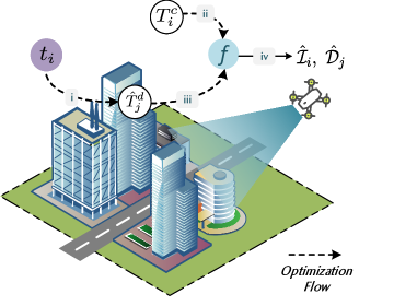
Figure 3: Optimization Pipeline. (i) the time-pose function learns the embedded trajectory prior from the RGB sequence and predicts the depth camera poses; (ii), (iii) the ground-truth RGB camera poses and the estimated depth camera poses are used in learning the 3D scene representation that generates observed RGB images and depth maps at novel perspective (iv).

We introduce in section 3.1 and 3.2 a method of generating initial poses of depth maps using an implicit time-pose function of the trajectory prior. The functional relationship is learned from the time-pose pairs in the RGB sequence. In section 3.3 we introduce our method for mapping and optimizing the predicted poses simultaneously.

3.1 Time-Pose Function

In this part, we introduce the time-pose function that estimates the camera poses.

We represent the camera trajectory as an implicit time-pose function whose input is a timestamp, and whose output is a 6-DoF camera pose. The pose output consists of a 3D translation vector $\hat{x}_{i}$ and a 4-D rotation vector represented as a quaternion $\hat{q}_{i}$.

Network Overview The time-pose function is approximated with a 1-dimensional multi-resolution hash grid $\{\mathcal{G}_{\theta}^{(l)}\}_{l=1}^{L}$, followed by an MLP structure $\mathcal{F}_{\Theta}$. The hash grid consists of $L$ levels of separate feature grids with trainable hash encodings[16].

When querying the camera pose $\mathbf{\hat{T}}_{i}$ for an arbitrary timestamp $t_{i}$ that is in the interval of the timestamps, we sample the hash encodings from each grid layer and perform quadratic interpolation on the extracted encodings to obtain a feature vector $\mathcal{V}_{i}$. After obtaining the interpolated feature vector, a shared MLP is used to process the input, whose output is then fed into two separated fully connected layers to predict the output translation $\hat{x}_{i}$ and rotation $\hat{q}_{i}$ vector respectively. The forward pass can be expressed in the following equations:

$$\mathcal{V}_{i} =\mathcal{F}_{\Theta}\left(\ \{\text{interp}(\text{h}(t_{i},\pi_{l}),\ \mathcal{G}_{\theta}^{l}\}_{l=1}^{L}\ \right),$$ (2)

$$\mathbf{\hat{T}}_{i} =[\hat{x}_{i},\hat{q}_{i}]=l_{\text{trans}}(\mathcal{V}_{i},\Theta_{\text{trans}}),\ l_{\text{rot}}(\mathcal{V}_{i},\Theta_{\text{rot}}),$$ (3)

where interp denotes the interpolation operator, h is the hash function parameterized by $\pi_{l}$, $l_{\text{trans}},l_{\text{rot}}$ are the two fully connected layer, where $\Theta_{\text{trans}},\Theta_{\text{rot}}$ represent the network parameters respectively.

Depth-pose Prediction Since both the depth maps and the RGB images are collected by the same drone in the same flight, they have an almost identical trajectory in temporal and spatial terms except for the difference in the placement of the two sensors on the aircraft. Therefore we can directly predict the poses corresponding to the depth sequence timestamps using the implicit time-pose function we learned in the RGB sequence with a pre-defined pose transformation $\textbf{T}_{\text{sensor}}$ between sensor positions.

3.2 Optimizing Time-Pose Function

The most common choices to represent rotation for optimizing camera poses are to use rotation matrices[35] or Euler-angles[26, 29]. However, they are not continuous for representing rotation[41] for their non-homeomorphic representation space to SO(3). We chose to use unit quaternion as our raw representation because arbitrary 4-D values are easily mapped to legitimate rotations by normalizing them to unit length[9].

To optimize the time-pose function, we propose the following objective function:

$$\mathcal{L}=\lambda_{\text{trans}}\mathcal{L}_{\text{trans}}+\lambda_{\text{rot}}\mathcal{L}_{\text{rot}}+\lambda_{\text{speed}}\mathcal{L}_{\text{speed}},$$ (4)

where $\lambda_{\text{trans}},\lambda_{\text{rot}},\lambda_{\text{grad}}$ are the weighting parameters.

Direct Optimization of Translation and Rotation We directly optimize the translation and the rotation vector in the Euclidean space by evaluating the mean square error (MSE) of the estimated camera poses and the ground-truth pose vectors:

$$\mathcal{L}_{\text{trans}} =\text{MSE}(x(\{t_{i}\}),\hat{x}(\{t_{i}\}))=\frac{1}{n}\sum_{i=1}^{n}(x_{i}-\hat{x}_{i})^{2},$$ (5)

$$\mathcal{L}_{\text{rot}} =\text{MSE}(q(\{t_{i}\}),\hat{q}(\{t_{i}\}))=\frac{1}{n}\sum_{i=1}^{n}(q_{i}-\hat{q}_{i})^{2}.$$ (6)

Since $x$ and $q$ are in different units, the scaling factor $\lambda_{\text{trans}}$ and $\lambda_{\text{rot}}$ played an important role to balance the losses. To prevent translation and rotation from influencing each other in training and to tap into possible mutual facilitation, we made the weighting factors learnable[8].

Gradient Optimization of Motion Speed Observing that the time-pose function is essentially a function of displacement and angular displacement with respect to time, we can use the average velocity calculated from the ground-truth camera pose to supervise the gradient of the network output. Since the velocity variation is small and the angular velocity variation is relatively larger in the scenes captured by the drone, only the average velocity is used to supervise the neural network:

$$\mathcal{L}_{\text{grad}}=\text{MSE}(v(t_{i}),\hat{v}(t_{i}))=\frac{1}{n}\sum_{i=1}^{n}(v(t_{i})-\frac{\partial\hat{x}}{\partial t}(t_{i}))^{2},$$ (7)

where $v(t_{i})=\left.\frac{\partial x}{\partial t}\right|_{t=t_{i}}\approx\frac{x_{i}-x_{i-1}}{t_{i}-t_{i-1}}$.

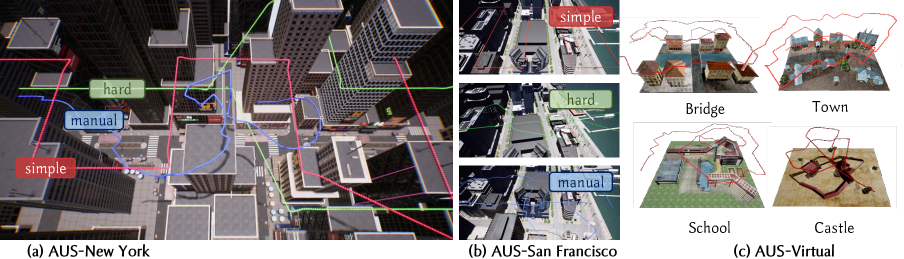
Figure 4: Visualization of our proposed AUS dataset

3.3 Learning Large-scale Implicit Fields with Joint Time-Pose Function Error Compensation

While the time-pose function provides a great initial value for the mapping stage, there still exists noticeable error in some of the outlying frames. In this section, we describe how we perform simultaneous mapping and pose optimization, which compensates for the error of the time-pose function. We partition the city scene map into a series of equal-sized blocks in terms of spatial scope, and each block learns its scene representation with an implicit field separately, while the camera poses $\hat{T}_{i}^{d}$ corresponding to the depth map is also optimized in the training process.

Scene Representation We represent the scene model as a series of implicit functions mapping from spatial point coordinates and viewing directions to the radiance values as $\{f_{\text{MLP}}^{(i)}\}_{i=1}^{N_{x}\times N_{y}}$, where $N_{x},N_{y}$ denotes the spatial grid size. Each implicit function represents a geographic region with $\textbf{x}_{i}^{\text{centroid}}$ as its centroid.

$$\vspace{-1mm}f^{\text{(k)}}_{\text{MLP}}(\gamma^{(\alpha)}(\mathbf{x}_{\text{pts}}),\mathbf{d},l^{(a)})\to(\hat{c},\sigma),$$ (8)

$$\text{where }\text{k}=\mathop{\arg\min}\limits_{j}||\mathbf{x}_{\text{pts}}-\mathbf{x}_{j}^{\text{centroid}}||_{2}.\vspace{-1mm}$$

For view synthesis, we adopt volume rendering techniques that are proven to be powerful. To be specific, we sample a set of points for each emitted camera ray in a coarse-to-fine manner [15] and accumulate the radiance and the ray-depth along the corresponding ray to calculate the rendered color $\mathcal{\hat{I}}$ and depth $\mathcal{\hat{D}}$. To obtain the radiance of a spatial point $\mathbf{x}_{\text{pts}}$, we use the nearest scene model for prediction. A set of per-image appearance embedding $l^{(a)}$ [14] is also optimized simultaneously in the training.

$$\mathcal{\hat{I}}(\mathbf{o},\mathbf{d}) =\int_{\text{near}}^{\text{far}}T(t)\sigma^{(k)}(\mathbf{x}(t))\cdot c^{(k)}(\mathbf{x}(t),\mathbf{d})\text{d}t,$$ (9)

$$\mathcal{\hat{D}}(\mathbf{o},\mathbf{d}) =\int_{\text{near}}^{\text{far}}T(t)\sigma^{(k)}(\mathbf{x}(t))\cdot t\text{d}t,$$ (10)

where o and d denote the position and orientation of the sampled ray, $\textbf{x}(t)=\textbf{o}+t\textbf{d}$ represents the sampled point coordinates in the world space, and $T(t)=\exp\left(-\int_{\text{near}}^{t}\sigma^{(k)}(\textbf{x}(s))\text{d}s\right)$ is the accumulated transmittance.

Optimization We jointly optimize the inaccurate camera poses and the scene mapping: When fitting parameters $\Theta_{\text{MLP}}^{(k)}$ of the scene representation, the estimated depth camera poses $\hat{T}_{i}\in SE(3)$ (where $t\in\mathbb{R}^{3}$ and $q\in SO(3)$) will be simultaneously optimized on the manifold:

$$\hat{\Theta}_{\text{MLP}},\mathbf{\hat{T}}=\underset{\textbf{T}\in SE(3),\Theta}{\operatorname{argmin}}\mathcal{L}(\textbf{T},{\Theta_{\text{MLP}}}\mid{\textbf{T}_{0}},\{\mathcal{I}_{i}\},\{\mathcal{D}_{i}\}),$$ (11)

where $\mathcal{L}$ is the objective function, and $\textbf{T}_{0}$ is the initial pose input from the time-pose function .

To train the implicit expression to obtain realistic RGB rendering maps and accurate depth map estimation, we used the objective function proposed in equation 12.

$$\mathcal{L}=\lambda_{\text{color}}\text{MSE}(\mathcal{I},\mathcal{\hat{I}})+\lambda_{\text{depth}}(\alpha_{0})\text{MSE}(\mathcal{D},\mathcal{\hat{D}}),$$ (12)

where $\lambda_{\text{color}}$ and $\lambda_{\text{depth}}(\alpha_{0})$ are weighting hyper-parameters for color and depth loss, in which the depth loss weight starts to grow from zero gradually with training process $\alpha_{0}$.

To compensate for the error from the time-pose function extracted poses, we further optimize the estimated poses $\mathbf{\hat{T}}$ by applying a set of trainable pose correction terms $\{\xi_{x}^{(i)},\xi_{q}^{(i)}\}$ (where $\xi_{q}^{(i)}\in\mathbb{R}^{3},\xi_{q}^{(i)}\in\mathfrak{so}(3)$) to the initial poses $\{\hat{x}_{0,i},\hat{q}_{0,i}\}$ in each iteration:

$$\hat{q}_{i}^{\prime} =\text{Exp}(\xi_{i})\cdot\hat{q}_{0,i},$$ (13)

$$\hat{x}_{i}^{\prime} =\xi_{x}^{(i)}+\hat{x}_{0,i}$$ (14)

where $\text{Exp}(\cdot)$ is the exponential mapping that uses the Rodrigues formula [20] to map rotation vectors in $\mathfrak{so}(3)$ to rotation matrices.

Dynamic Low-pass Filter As stated in BARF[11], in solving the positional calibration problem, smoother signals can predict more consistent displacements than complex signals, which can easily lead to sub-optimal optimization results. The positional encoding in the traditional NeRF rendering significantly improves the synthesized view in terms of high-frequency details. Using a low-pass filter that can weaken the effect of position coding will have a similar effect as smoothing. Thus, a dynamic low-pass filter is used in AsyncNeRF in the joint-optimization stage to help optimize inaccurate depth frame poses.

Scene	Method	Time-Pose Function		Novel-view Synthesis				Depth Estimation						Pose Optimization
		Rotation$(^{\circ})$ $\downarrow$	Translation $(m)\downarrow$		PSNR $\uparrow$	SSIM $\uparrow$	LPIPS $\downarrow$		RMSE $\downarrow$	RMSE log $\downarrow$	$\delta_{1}\uparrow$	$\delta_{2}\uparrow$	$\delta_{3}\uparrow$	Rotation $(^{\circ})\downarrow$	Translation $(m)\downarrow$
NY simple	NeRF-W				23.06	0.7946	0.2318		16.74	0.2149	84.62%	93.99%	99.68%
	Mega-NeRF	0.6601	1.8400		23.48	0.8744	0.1738		19.74	0.2411	82.76%	93.25%	96.71%	0.1336	0.3394
	Ours				24.77	0.8469	0.1661		5.50	0.0690	97.78%	99.39%	99.85%
NY hard	NeRF-W				22.88	0.7899	0.2574		9.97	0.2027	86.04%	94.63%	97.31%
	Mega-NeRF	0.5908	1.1200		23.09	0.7860	0.2339		10.07	0.2117	87.59%	95.64%	97.47%	0.0890	0.5644
	Ours				23.99	0.8162	0.2218		7.03	0.1672	94.91%	97.21%	98.33%
NY Manual	NeRF-W				24.02	0.8471	0.1854		25.48	0.3715	69.85%	81.71%	87.18%
	Mega-NeRF	3.6980	0.4605		24.03	0.8522	0.1683		42.15	0.43	69.99%	77.43%	84.43%	1.4740	0.1997
	Ours				24.24	0.8406	0.1621		5.93	0.0085	91.85%	98.08%	99.48%
SF simple	NeRF-W				22.12	0.8297	0.2528		31.12	0.1988	86.14%	90.59%	98.17%
	Mega-NeRF	0.1700	1.3380		19.99	0.8294	0.2252		32.17	0.2188	86.38%	92.12%	95.04%	0.0465	0.3193
	Ours				22.70	0.8336	0.2067		7.26	0.0669	97.97%	99.30%	99.72%
SF hard	NeRF-W				17.17	0.5564	0.4489		23.58	0.1429	81.14%	91.36%	96.34%
	Mega-NeRF	0.6656	1.4488		19.77	0.7112	0.3302		26.02	0.1666	86.20%	94.92%	96.45%	0.4064	1.0880
	Ours				20.49	0.7164	0.3344		9.99	0.0992	93.68%	97.78%	99.72%
SF Manual	NeRF-W				18.33	0.5968	0.3878		20.09	0.2214	78.14%	92.67%	96.29%
	Mega-NeRF	0.6539	0.9393		21.83	0.6596	0.2304		12.48	0.1286	93.17%	97.18%	99.01%	0.0191	0.6632
	Ours				23.24	0.8291	0.2450		5.66	0.0706	97.37%	99.31%	99.67%
Bridge	NeRF-W				26.79	0.8053	0.2438		131.88	1.2277	53.76%	61.57%	58.98%
	Mega-NeRF	1.5108	0.9514		27.98	0.8674	0.1548		120.41	1.3246	69.10%	72.54%	73.17%	0.4893	0.5709
	Ours				29.06	0.8751	0.1952		26.56	0.3248	93.24%	96.32%	98.26%
Town	NeRF-W				21.32	0.6208	0.4088		132.70	1.4640	44.89%	55.68%	57.90%
	Mega-NeRF	0.6774	1.3460		24.69	0.7305	0.3103		129.50	1.4240	54.54%	59.18%	57.90%	0.3633	0.8364
	Ours				25.32	0.7675	0.2631		15.61	0.4632	91.92%	96.89%	98.49%
School	NeRF-W				19.69	0.5715	0.44527		88.83	0.9365	61.73%	72.58%	75.80%
	Mega-NeRF	0.7031	0.8780		25.57	0.7739	0.3191		63.10	0.7651	77.18%	85.02%	86.69%	0.6807	0.5600
	Ours				26.51	0.7971	0.3175		21.19	0.2083	92.87%	95.78%	97.51%
Castle	NeRF-W				22.63	0.7443	0.2557		78.18	0.8651	75.72%	79.26%	81.11%
	Mega-NeRF	1.0525	0.3772		28.06	0.9053	0.1159		54.99	0.6167	79.69%	83.59%	87.43%	0.3822	0.1200
	Ours				28.21	0.8976	0.1113		16.66	0.3565	93.12%	97.23%	98.45%

Table 1: Quantitative results on the localization quality of the time-pose Function, the mapping quality, and the effect of the pose optimization in the mapping stage. The time-pose function successfully localized the depth camera poses. The scene representation network achieves high-quality novel view synthesis results and accurate depth estimation while further compensating for the depth pose error.

4 Experiments

In this section, we show in the effectiveness of our two-staged pipeline. We first introduce the experiment setup in section 4.1 and 4.2. In section 4.3, we qualitatively and quantitatively evaluate our proposed methods.

4.1 Datasets

We evaluate our method against our proposed Asynchronous Urban Scene (AUS) dataset (Figure 4). The AUS dataset is generated from a simulator. With loaded scene models, the simulator can create asynchronous RGB-D sequences that mimic real-world asynchronous sequences. The proposed dataset consists of 2 realistic scenes and 4 virtual scenes. The former uses the New York and San Francisco city scenes provided by Kirill Sibiriakov[25], in which AUS-NewYork covers a $250\times 150m^{2}$ area with many detailed buildings and AUS-SanFrancisco consists of a $500\times 250m^{2}$ area near the Golden Gate Bridge, while the latter uses the simulation model files provided in the UrbanScene3D dataset [13]. We make use of the physical engine of Unreal Engine together with AirSim[23] to model physical properties and use three types of trajectory which consists of a Zig-Zag trajectory, a more complex planned random trajectory, and a complex manual controlled trajectory. In virtual scenes, we only provide manually controlled trajectories, since the scene sizes are relatively smaller.

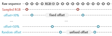
Figure 5: Visual demonstration of the sampling strategies. We sample one RGB frame from every 5 frames of raw RGB-D data. We calculate the depth frame sampling time by adding different offsets to the RGB frame timestamps. Two types of offsets are included in the AUS dataset: (1) fixed offsets of 10%-50% of the time interval between two adjacent RGB frames (5 traces in total); (2) unfixed offset by random.

In real scenarios, RGB cameras and LiDAR are usually not aligned in time, so we sample raw RGB-D sequences in the simulator at a higher frequency (50fps) and re-sampled them with different starting frames to get similar asynchronous RGB-D sequences. To further increase the realism, we added random perturbations to the fixed offsets. The sampling method is shown in figure 5.

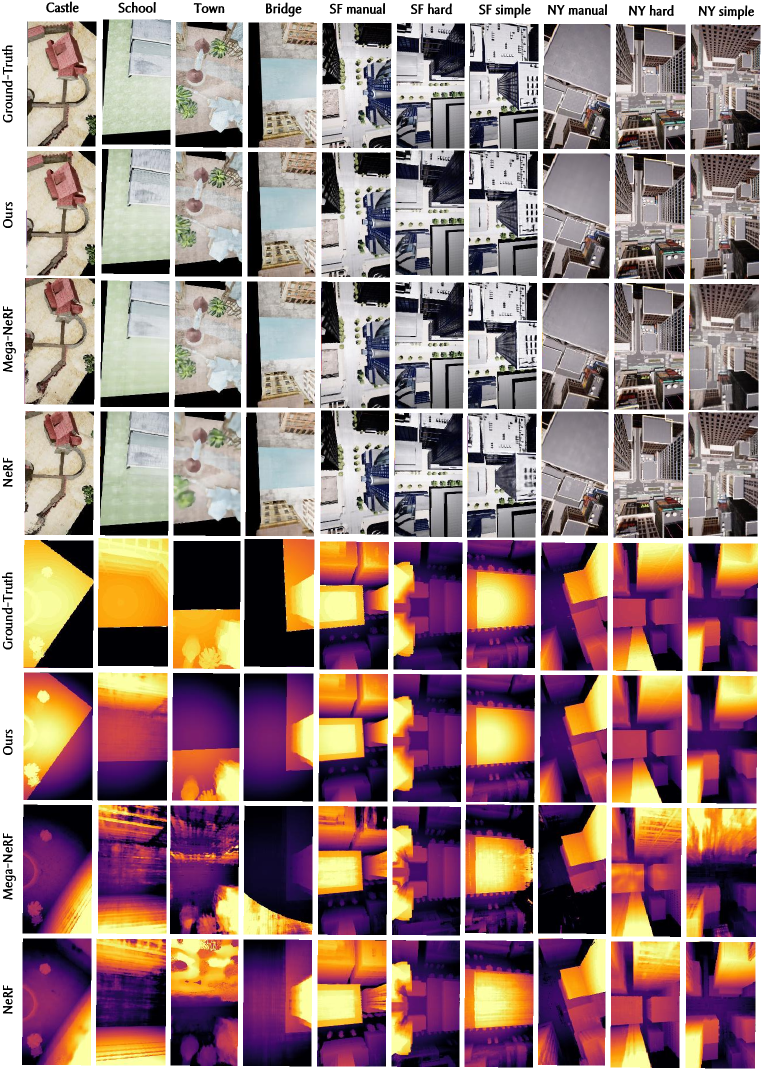
Figure 6: Qualitative Results. Async-NeRF can render photo-realistic novel views and the best depth estimation results.

4.2 Implementation Details

Time-Pose Function In our experiments, we maintain a multi-resolution feature grid with $L=2$, concatenate the interpolated feature vectors from different grid layers together and process through a shallow MLP of 5 layers with 1024 neurons in each layer. We use a spatial hash function $h^{(l)}(x)=\left\lfloor x\right\rfloor\oplus\pi_{l}\ \text{mod}\ N_{l}$ for each layer of the grid, where $\oplus$ denotes the bit-wise XOR operation, $N_{l}$ is the number of feature vectors in layer $l$, and $\pi_{l}$ is the selected large prime number. In our experiments, we set $\pi_{0}=1,\pi_{1}=2,654,435,761$. We use the Adam[10] optimizer with an initial learning rate of $5\times 10^{-4}$ decaying exponentially to $5\times 10^{-5}$. The initial weighting parameters for optimizing the time-pose function are set to a default of $\lambda_{\text{trans}}=1,\lambda_{\text{rot}}=1$, and $\lambda_{\text{speed}}=10^{-3}$.

Joint Optimization We follow the spatial partitioning method from Mega-NeRF[30]. We train all models for 500K iterations and render a batch of 1024 rays at each step, with a learning rate of $5\times 10^{-4}$ decaying to $5\times 10^{-5}$ for the scene representation networks, and $1\times 10^{-6}$ decaying to $1\times 10^{-7}$ for the pose optimization. The hyper-parameters for each loss in this stage are set to $\lambda_{\text{color}}=1$, and $\lambda_{\text{depth}}(\alpha_{0})=10^{-3}\cdot\alpha_{0}$.

4.3 Results

We evaluate our proposed Async-NeRF against NeRFW[14] and city-scale Mega-NeRF [30]. We present the quantitative results in table 1.

Time-Pose Function We evaluate pose error to demonstrate the ability of the time-pose function to localize from time-pose sequences. As shown in the table, our methods can achieve an average pose accuracy of less than $1.5m$ in translation and $2^{\circ}$ in rotation.

Mapping The standard metrics for novel view synthesis and depth estimation are used for evaluation. For view synthesis, metrics including PSNR, SSIM, and the VGG implementation of LPIPS [39] is used. For depth estimation, RMSE, RMSE log, $\delta_{1}$, $\delta_{2}$, and $\delta_{3}$ are used. We also present the mapping results qualitatively in figure 6. We show that our methods can synthesize photo-realistic novel views with comparable quality to the recent state-of-the-art methods. Our method significantly outperforms current RGB-based methods for depth estimation.

4.4 Ablation Studies

Time-Pose Function Network Structure We evaluate our methods against different network structures on localization accuracy: (a)Pure MLP structure: straightly process the input timestamps with an MLP. (b)1-D Feature Grid: maintain a feature vector for each second in the timestamp span. (c)Ours: our proposed 1-D multi-resolution hash grid with different layers of resolution.

The results (Table 2) show that our proposed multi-resolution outperforms other network structures in accuracy.

Ablation of the Speed Optimization We compared the localization accuracy and optimization time of our method with and without the gradient optimization of motion speed. Quantitative results are listed in table 2.

Method	rotation ∘		translation $m$
	mean	median	mean	median
MLP	26.62	17.53	8.23	7.5
Feature Grid	15.86	14.56	8.53	7.48
Ours (L=1)	24.24	12.99	9.2	8.01
Ours w/o speed constraint	12.96	11.21	19.95	12.28
Ours	11.36	11.17	6.29	4.03

Table 2: Result of the ablation on different network structures and the use of speed optimization

Scene	Ours		Mega-NeRF		Mega-NeRF-Depth
	PSNR	RMSE	PSNR	RMSE	PSNR	RMSE
NY	24.24	5.93	24.025	42.15	19.701	15.94
SF	22.6985	7.26	19.9957	32.1686	19.0666	11.3864
Bridge	29.0644	26.55	27.9767	120.41	22.3456	96.16
Town	25.315	15.61	24.6925	129.5	20.135	81.99
School	26.51	21.192	25.5729	63.1047	21.9129	42.74
Castle	28.2157	16.6617	28.0643	54.9895	23.23	38.8983

Table 3: Result of the ablation of error compensation

Ablation of Pose Error Compensation We train a Mega-NeRF[30] with depth supervision from the ground-truth depth maps and the depth camera pose output from the time-pose function and compare its mapping results with our proposed method. From the evaluation results (Table 3), we find that depth supervision with errors can improve Mega-NeRF’s effectiveness on depth prediction, but incorrect geometric information in turn affects the performance of the rendering network.

offset	rotation ∘			translation $m$
	mean	median		mean	median
10%	0.6578	0.2590		3.4248	1.8818
20%	0.9422	0.5516		4.9643	3.898
30%	1.2383	0.7914		6.4142	5.7807
40%	1.4141	0.7538		7.2644	6.617
50%	1.4984	0.8419		5.1704	6.5162
random	1.1228	0.5155		5.1704	4.0544

Table 4: Result of the ablation of different sampling offset

Ablation of Different Sampling Offset We compare the localization accuracy of implicit trajectory representations trained with RGB poses in predicting depth camera poses under different sampling offsets. We trained a time-pose function with a sparse set of time-pose pairs to amplify the differences in quantitative results (Table 4).

5 Conclusion

We present Async-NeRF, a pipeline that uses an implicit functional relationship between time-pose to calibrate RGB-D poses and train a large-scale implicit scene representation. Our experiments show that Async-NeRF can effectively register depth camera poses by leveraging the trajectory prior embedded in RGB time-pose relationship. Meantime, Async-NeRF learns the 3D scene representation for photo-realistic novel view synthesis and accurate depth estimations.

References

- [1] Dejan Azinović, Ricardo Martin-Brualla, Dan B Goldman, Matthias Nießner, and Justus Thies. Neural rgb-d surface reconstruction. In Proceedings of the IEEE/CVF Conference on Computer Vision and Pattern Recognition, pages 6290–6301, 2022.
- [2] Jonathan T Barron, Ben Mildenhall, Matthew Tancik, Peter Hedman, Ricardo Martin-Brualla, and Pratul P Srinivasan. Mip-nerf: A multiscale representation for anti-aliasing neural radiance fields. In Proceedings of the IEEE/CVF International Conference on Computer Vision, pages 5855–5864, 2021.
- [3] Carlos Campos, Richard Elvira, Juan J. Gómez Rodríguez, José M. M. Montiel, and Juan D. Tardós. ORB-SLAM3: An Accurate Open-Source Library for Visual, Visual–Inertial, and Multimap SLAM. IEEE Transactions on Robotics, 37(6):1874–1890, Dec. 2021.
- [4] Kangle Deng, Andrew Liu, Jun-Yan Zhu, and Deva Ramanan. Depth-supervised NeRF: Fewer Views and Faster Training for Free. In 2022 IEEE/CVF Conference on Computer Vision and Pattern Recognition (CVPR), pages 12872–12881, June 2022.
- [5] Jakob Engel, Vladlen Koltun, and Daniel Cremers. Direct Sparse Odometry. IEEE Transactions on Pattern Analysis and Machine Intelligence, 40(3):611–625, Mar. 2018.
- [6] Jakob Engel, Thomas Schöps, and Daniel Cremers. Lsd-slam: Large-scale direct monocular slam. In European conference on computer vision, pages 834–849. Springer, 2014.
- [7] Yoonwoo Jeong, Seokjun Ahn, Christopher Choy, Animashree Anandkumar, Minsu Cho, and Jaesik Park. Self-Calibrating Neural Radiance Fields. In 2021 IEEE/CVF International Conference on Computer Vision (ICCV), pages 5826–5834, Oct. 2021.
- [8] Alex Kendall and Roberto Cipolla. Geometric loss functions for camera pose regression with deep learning. In Proceedings of the IEEE conference on computer vision and pattern recognition, pages 5974–5983, 2017.
- [9] Alex Kendall, Matthew Grimes, and Roberto Cipolla. Posenet: A convolutional network for real-time 6-dof camera relocalization. In Proceedings of the IEEE international conference on computer vision, pages 2938–2946, 2015.
- [10] Diederik P. Kingma and Jimmy Ba. Adam: A method for stochastic optimization. CoRR, abs/1412.6980, 2015.
- [11] Chen-Hsuan Lin, Wei-Chiu Ma, Antonio Torralba, and Simon Lucey. BARF: Bundle-Adjusting Neural Radiance Fields. In Proceedings of the IEEE/CVF International Conference on Computer Vision, pages 5741–5751, 2021.
- [12] Philipp Lindenberger, Paul-Edouard Sarlin, Viktor Larsson, and Marc Pollefeys. Pixel-Perfect Structure-from-Motion with Featuremetric Refinement. In ICCV, 2021.
- [13] Yilin Liu, Fuyou Xue, and Hui Huang. Urbanscene3d: A large scale urban scene dataset and simulator. CoRR, abs/2107.04286, 2021.
- [14] Ricardo Martin-Brualla, Noha Radwan, Mehdi S. M. Sajjadi, Jonathan T. Barron, Alexey Dosovitskiy, and Daniel Duckworth. NeRF in the Wild: Neural Radiance Fields for Unconstrained Photo Collections. In 2021 IEEE/CVF Conference on Computer Vision and Pattern Recognition (CVPR), pages 7206–7215, June 2021.
- [15] Ben Mildenhall, Pratul P. Srinivasan, Matthew Tancik, Jonathan T. Barron, Ravi Ramamoorthi, and Ren Ng. NeRF: Representing Scenes as Neural Radiance Fields for View Synthesis. In Andrea Vedaldi, Horst Bischof, Thomas Brox, and Jan-Michael Frahm, editors, Computer Vision – ECCV 2020, Lecture Notes in Computer Science, pages 405–421, Cham, 2020. Springer International Publishing.
- [16] Thomas Müller, Alex Evans, Christoph Schied, and Alexander Keller. Instant neural graphics primitives with a multiresolution hash encoding. ACM Transactions on Graphics, 41(4):1–15, July 2022.
- [17] Raúl Mur-Artal, J. M. M. Montiel, and Juan D. Tardós. ORB-SLAM: A Versatile and Accurate Monocular SLAM System. IEEE Transactions on Robotics, 31(5):1147–1163, Oct. 2015.
- [18] Matthias Nießner, Michael Zollhöfer, Shahram Izadi, and Marc Stamminger. Real-time 3D reconstruction at scale using voxel hashing. ACM Transactions on Graphics, 32(6):169:1–169:11, Nov. 2013.
- [19] Konstantinos Rematas, Andrew Liu, Pratul Srinivasan, Jonathan Barron, Andrea Tagliasacchi, Thomas Funkhouser, and Vittorio Ferrari. Urban Radiance Fields. In 2022 IEEE/CVF Conference on Computer Vision and Pattern Recognition (CVPR), pages 12922–12932, June 2022.
- [20] Rodrigues. Des lois géométriques qui régissent les déplacements d’un système solide dans l’espace, et de la variation des coordonnées provenant de ces déplacements considérés indépendamment des causes qui peuvent les produire. Journal de Mathématiques Pures et Appliquées, pages 380–440, 1840.
- [21] Barbara Roessle, Jonathan T. Barron, Ben Mildenhall, Pratul P. Srinivasan, and Matthias Nießner. Dense Depth Priors for Neural Radiance Fields from Sparse Input Views. In 2022 IEEE/CVF Conference on Computer Vision and Pattern Recognition (CVPR), pages 12882–12891. IEEE Computer Society, June 2022.
- [22] Johannes Lutz Schönberger and Jan-Michael Frahm. Structure-from-Motion Revisited. In Conference on Computer Vision and Pattern Recognition (CVPR), 2016.
- [23] Shital Shah, Debadeepta Dey, Chris Lovett, and Ashish Kapoor. Airsim: High-fidelity visual and physical simulation for autonomous vehicles. CoRR, abs/1705.05065, 2017.
- [24] Tixiao Shan, Brendan Englot, Carlo Ratti, and Daniela Rus. Lvi-sam: Tightly-coupled lidar-visual-inertial odometry via smoothing and mapping. In 2021 IEEE international conference on robotics and automation (ICRA), pages 5692–5698. IEEE, 2021.
- [25] Kirill Sibiriakov. Artstation page https://www.artstation.com/vegaart, 2022.
- [26] Hao Su, Charles R Qi, Yangyan Li, and Leonidas J Guibas. Render for cnn: Viewpoint estimation in images using cnns trained with rendered 3d model views. In Proceedings of the IEEE international conference on computer vision, pages 2686–2694, 2015.
- [27] Edgar Sucar, Shikun Liu, Joseph Ortiz, and Andrew J Davison. imap: Implicit mapping and positioning in real-time. In Proceedings of the IEEE/CVF International Conference on Computer Vision, pages 6229–6238, 2021.
- [28] Matthew Tancik, Vincent Casser, Xinchen Yan, Sabeek Pradhan, Ben P. Mildenhall, Pratul Srinivasan, Jonathan T. Barron, and Henrik Kretzschmar. Block-NeRF: Scalable Large Scene Neural View Synthesis. In 2022 IEEE/CVF Conference on Computer Vision and Pattern Recognition (CVPR), pages 8238–8248, June 2022.
- [29] Shubham Tulsiani and Jitendra Malik. Viewpoints and keypoints. In Proceedings of the IEEE Conference on Computer Vision and Pattern Recognition, pages 1510–1519, 2015.
- [30] Haithem Turki, Deva Ramanan, and Mahadev Satyanarayanan. Mega-NeRF: Scalable Construction of Large-Scale NeRFs for Virtual Fly- Throughs. In 2022 IEEE/CVF Conference on Computer Vision and Pattern Recognition (CVPR), pages 12912–12921, June 2022.
- [31] Rui Wang, Martin Schworer, and Daniel Cremers. Stereo dso: Large-scale direct sparse visual odometry with stereo cameras. In Proceedings of the IEEE International Conference on Computer Vision, pages 3903–3911, 2017.
- [32] Zirui Wang, Shangzhe Wu, Weidi Xie, Min Chen, and Victor Adrian Prisacariu. NeRF: Neural radiance fields without known camera parameters. arXiv preprint arXiv:2102.07064, 2021.
- [33] Yuanbo Xiangli, Linning Xu, Xingang Pan, Nanxuan Zhao, Anyi Rao, Christian Theobalt, Bo Dai, and Dahua Lin. BungeeNeRF: Progressive Neural Radiance Field for Extreme Multi-scale Scene Rendering, July 2022.
- [34] Yi Xu, Yuzhang Wu, and Hui Zhou. Multi-scale Voxel Hashing and Efficient 3D Representation for Mobile Augmented Reality. In 2018 IEEE/CVF Conference on Computer Vision and Pattern Recognition Workshops (CVPRW), pages 1586–15867, June 2018.
- [35] Lin Yen-Chen, Pete Florence, Jonathan T. Barron, Alberto Rodriguez, Phillip Isola, and Tsung-Yi Lin. iNeRF: Inverting Neural Radiance Fields for Pose Estimation. In 2021 IEEE/RSJ International Conference on Intelligent Robots and Systems (IROS), pages 1323–1330, Sept. 2021.
- [36] Aviad Zabatani, Vitaly Surazhsky, Erez Sperling, Sagi Ben Moshe, Ohad Menashe, David H. Silver, Zachi Karni, Alexander M. Bronstein, Michael M. Bronstein, and Ron Kimmel. Intel® RealSense™ SR300 Coded Light Depth Camera. IEEE Transactions on Pattern Analysis and Machine Intelligence, 42(10):2333–2345, Oct. 2020.
- [37] Ji Zhang and Sanjiv Singh. Laser–visual–inertial odometry and mapping with high robustness and low drift. Journal of field robotics, 35(8):1242–1264, 2018.
- [38] Kai Zhang, Gernot Riegler, Noah Snavely, and Vladlen Koltun. Nerf++: Analyzing and improving neural radiance fields. arXiv preprint arXiv:2010.07492, 2020.
- [39] Richard Zhang, Phillip Isola, Alexei A. Efros, Eli Shechtman, and Oliver Wang. The Unreasonable Effectiveness of Deep Features as a Perceptual Metric. In 2018 IEEE/CVF Conference on Computer Vision and Pattern Recognition, pages 586–595, June 2018.
- [40] Zhengyou Zhang. Microsoft Kinect Sensor and Its Effect. IEEE Multimedia, 19(2):4–10, Feb. 2012.
- [41] Yi Zhou, Connelly Barnes, Jingwan Lu, Jimei Yang, and Hao Li. On the continuity of rotation representations in neural networks. In Proceedings of the IEEE/CVF Conference on Computer Vision and Pattern Recognition, pages 5745–5753, 2019.
- [42] Yuewen Zhu, Chunran Zheng, Chongjian Yuan, Xu Huang, and Xiaoping Hong. Camvox: A low-cost and accurate lidar-assisted visual slam system. In 2021 IEEE International Conference on Robotics and Automation (ICRA), pages 5049–5055. IEEE, 2021.
- [43] Zihan Zhu, Songyou Peng, Viktor Larsson, Weiwei Xu, Hujun Bao, Zhaopeng Cui, Martin R. Oswald, and Marc Pollefeys. NICE-SLAM: Neural Implicit Scalable Encoding for SLAM. In 2022 IEEE/CVF Conference on Computer Vision and Pattern Recognition (CVPR), pages 12776–12786, June 2022.