Abstract

We find a large class of new supersymmetric $AdS_{5}$ black strings from five-dimensional $N=4$ gauged supergravity coupled to five vector multiplets with $SO(2)_{D}\times SO(3)\times SO(3)$ gauge group. These solutions have near horizon geometries of the form $AdS_{3}\times\Sigma^{2}$ for $\Sigma^{2}$ being a two-sphere ($S^{2}$) or a hyperbolic space ($H^{2}$). There are four supersymmetric $AdS_{5}$ vacua with $N=4$ and $N=2$ supersymmetries. By performing topological twists along $\Sigma^{2}$ with $SO(2)\times SO(2)_{\textrm{diag}}$ and $SO(2)_{\textrm{diag}}$ gauge fields, we find a number of $AdS_{3}\times\Sigma^{2}$ fixed points describing near horizon geometries of black strings in asymptotically $AdS_{5}$ spaces. Most of the solutions take the form of $AdS_{3}\times H^{2}$ with only one being $AdS_{3}\times S^{2}$ preserving $SO(2)_{\textrm{diag}}$ symmetry. We also give the corresponding black string solutions interpolating between asymptotically locally $AdS_{5}$ vacua and the near horizon $AdS_{3}\times\Sigma^{2}$ geometries. There are a number of solutions flowing from one, two or three $AdS_{5}$ vacua to an $AdS_{3}\times\Sigma^{2}$ fixed point. These solutions can also be considered as holographic RG flows across dimensions from $N=2$ and $N=1$ SCFTs in four dimensions to two-dimensional SCFTs with $N=(2,0)$ or $N=(0,2)$ supersymmetry.

1 Introduction

Supersymmetric black hole solutions in asymptotically $AdS$ spaces have attracted much attention recently since the groundbreaking work on microstate counting of $AdS_{4}$ black holes from supersymmetric localization in [1], see also [2, 3, 4, 5, 6, 7, 8, 9, 10]. This technique has also been extended to supersymmetric $AdS_{5}$ black strings in [11, 12, 13, 14]. Due to these results, constructing new supersymmetric $AdS_{5}$ black string solutions to further test the proposed holographic relation is interesting. Along this line, gauged supergravities in five dimensions provide a very useful tool in which $AdS_{5}$ black strings become domain walls interpolating between asymptotically $AdS_{5}$ spaces and near horizon geometries of the form $AdS_{3}\times\Sigma^{2}$ for $\Sigma^{2}$ being a two-sphere ($S^{2}$) or a two-dimensional hyperbolic space ($H^{2}$).
On the other hand, supersymmetric $AdS_{5}$ black string solutions also describe holographic RG flows from four-dimensional superconformal field theories (SCFTs) in the UV, dual to $AdS_{5}$ vacua, to two-dimensional SCFTs in the IR dual to near horizon geometries [15]. In this point of view, the SCFTs in four dimensions undergo twisted compactifications on $\Sigma^{2}$ to conformal field theories in two dimensions. Since the pioneering work [15], a number of similar solutions have been found [16, 17, 18, 32, 33, 21, 22, 23, 24, 25, 26, 27, 28]. Some of the solutions can be uplifted to string/M-theory, and the SCFTs dual to these solutions have also been identified.
In this paper, we will look for new supersymmetric $AdS_{5}$ black string solutions from five-dimensional $N=4$ gauged supergravity with $SO(2)_{D}\times SO(3)\times SO(3)$ gauge group. This gauged supergravity can be constructed from $N=4$ supergravity coupled to five vector multiplets and has been studied recently in [29] in which a number of $N=2$ and $N=4$ supersymmetric $AdS_{5}$ vacua and holographic RG flows interpolating among them have been found. Similar solutions within the framework of $N=4$ gauged supergravity have also appeared in [27, 28], see [30, 31, 32, 33, 34, 35, 36] for $AdS$ black string solutions in higher dimensions.
Unlike the solutions given in [27, 28], due to a richer structure of $AdS_{5}$ vacua in the gauged supergravity considered in the present paper, there is a large number of new and more interesting $AdS_{5}$ black string solutions. In particular, there are solutions connecting one, two or three $AdS_{5}$ critical points to $AdS_{3}\times\Sigma^{2}$ fixed points. A truncation of this $SO(2)_{D}\times SO(3)\times SO(3)$ gauged supergravity to two or three vector multiplets and $SO(2)_{D}\times SO(3)$ gauge group can be embedded in eleven dimensions as shown in [37]. Accordingly, both the $AdS_{5}$ vacua and $AdS_{5}$ black strings within this truncation could be uplifted to higher dimensions leading to new $AdS_{5}$ and $AdS_{3}$ solutions of string/M-theory. However, apart from the proof of the consistency of the truncation using the powerful framework of exceptional field theories in [37], no complete truncation ansatze in this case have appeared to date.
The paper is organized as follows. In section 2, we review the construction of five-dimensional $N=4$ gauged supergravity with $SO(2)_{D}\times SO(3)\times SO(3)$ gauge group in the embedding tensor formalism. In sections 3 and 4, we give $AdS_{3}\times\Sigma^{2}$ geometries with $SO(2)_{\textrm{diag}}\times SO(2)$ and $SO(2)_{\textrm{diag}}$ symmetries together with black string solutions interpolating between these geometries and supersymmetric $AdS_{5}$ vacua. We end the paper with some conclusions and comments in section 5.

2 Five dimensional $N=4$ gauged supergravity with $SO(2)_{D}\times SO(3)\times SO(3)$ gauge group

In this section, we review $N=4$ gauged supergravity as constructed in [38, 39] by using the embedding tensor formalism. The supergravity multiplet consists of the graviton $e^{\hat{\mu}}_{\mu}$, four gravitini $\psi_{\mu i}$, six vectors $(A^{0}_{\mu},A_{\mu}^{m})$, four spin-$\frac{1}{2}$ fields $\chi_{i}$ and one real scalar $\Sigma$ or the dilaton. Space-time and tangent space indices are denoted respectively by $\mu,\nu,\ldots=0,1,2,3,4$ and $\hat{\mu},\hat{\nu},\ldots=0,1,2,3,4$. The fundamental representation of $SO(5)_{R}\sim USp(4)_{R}$ R-symmetry is described by $m,n=1,\ldots,5$ for $SO(5)_{R}$ and $i,j=1,2,3,4$ for $USp(4)_{R}$. A vector multiplet contains a vector field $A_{\mu}$, four gaugini $\lambda_{i}$ and five scalars $\phi^{m}$. For $N=4$ supergravity coupled to $n$ vector multiplets, we will label these multiplets by indices $a,b=1,\ldots,n$ of the form $(A^{a}_{\mu},\lambda^{a}_{i},\phi^{ma})$.
From the gravity and vector multiplets, there are $6+n$ vector fields denoted collectively by $A^{\mathcal{M}}_{\mu}=(A^{0}_{\mu},A^{m}_{\mu},A^{a}_{\mu})$ and $5n+1$ scalars in the $SO(1,1)\times SO(5,n)/SO(5)\times SO(n)$ coset manifold. For later convenience, we have introduced an index $\mathcal{M}=(0,M)$ as in [38]. The $5n$ scalars parametrizing the $SO(5,n)/SO(5)\times SO(n)$ coset can be described by a coset representative $\mathcal{V}_{M}^{\phantom{M}A}$ transforming under the global $G=SO(5,n)$ and the local $H=SO(5)\times SO(n)$ by left and right multiplications, respectively. We use the global $SO(5,n)$ indices $M,N,\ldots=1,2,\ldots,5+n$ while the local $H$ indices $A,B,\ldots$ can be split as $A=(m,a)$. The coset representative can then be written as

$$\mathcal{V}_{M}^{\phantom{M}A}=(\mathcal{V}_{M}^{\phantom{M}m},\mathcal{V}_{M}^{\phantom{M}a}).$$ (1)

For later convenience, we also define a symmetric matrix

$$M_{MN}=\mathcal{V}_{M}^{\phantom{M}m}\mathcal{V}_{N}^{\phantom{M}m}+\mathcal{V}_{M}^{\phantom{M}a}\mathcal{V}_{N}^{\phantom{M}a}$$ (2)

which is manifestly $SO(5)\times SO(n)$ invariant. Finally, all fermionic fields are symplectic Majorana spinors subject to the condition

$$\xi_{i}=\Omega_{ij}C(\bar{\xi}^{j})^{T}$$ (3)

with $C$ and $\Omega_{ij}$ being the charge conjugation matrix and $USp(4)$ symplectic matrix, respectively.
Gaugings of $N=4$ supergravity are characterized by the embedding tensor with components $\xi^{M}$, $\xi^{MN}=\xi^{[MN]}$ and $f_{MNP}=f_{[MNP]}$. These components determine the embedding of gauge groups in the global symmetry group $SO(1,1)\times SO(5,n)$. We are only interested in gaugings with $\xi^{M}=0$ which admit supersymmetric $AdS_{5}$ vacua as shown in [40]. Accordingly, we will set $\xi^{M}=0$ which leads to considerable simplification in various expressions. In particular, the quadratic constraints on the embedding tensor simply reduce to

$$f_{R[MN}{f_{PQ]}}^{R}=0\qquad\textrm{and}\qquad{\xi_{M}}^{Q}f_{QNP}=0\,.$$ (4)

Furthermore, for $\xi^{M}=0$, the gauge group is embedded solely in $SO(5,n)$ with the corresponding gauge generators in $SO(5,n)$ fundamental representation given by

$${(X_{M})_{N}}^{P}=-{f_{M}}^{QR}{(t_{QR})_{N}}^{P}={f_{MN}}^{P}\quad\textrm{and}\quad{(X_{0})_{N}}^{P}=-\xi^{QR}{(t_{QR})_{N}}^{P}={\xi_{N}}^{P}\,.$$ (5)

We have chosen $SO(5,n)$ generators of the form ${(t_{MN})_{P}}^{Q}=\delta^{Q}_{[M}\eta_{N]P}$ with $\eta_{MN}=\textrm{diag}(-1,-1,-1,-1,-1,1,1,\ldots,1)$ being the $SO(5,n)$ invariant tensor. The gauge covariant derivative reads

$$D_{\mu}=\nabla_{\mu}+A_{\mu}^{M}X_{M}+A^{0}_{\mu}X_{0}=\nabla_{\mu}+A^{\mathcal{M}}X_{\mathcal{M}}$$ (6)

with $\nabla_{\mu}$ being a space-time covariant derivative (possibly) including $SO(5)\times SO(n)$ composite connection.
The bosonic Lagrangian of a general gauged $N=4$ supergravity can be written as

$$e^{-1}\mathcal{L} = \frac{1}{2}R-\frac{3}{2}\Sigma^{-2}D_{\mu}\Sigma D^{\mu}\Sigma+\frac{1}{16}D_{\mu}M_{MN}D^{\mu}M^{MN}-V$$ (7)

$$-\frac{1}{4}\Sigma^{2}M_{MN}\mathcal{H}^{M}_{\mu\nu}\mathcal{H}^{N\mu\nu}-\frac{1}{4}\Sigma^{-4}\mathcal{H}^{0}_{\mu\nu}\mathcal{H}^{0\mu\nu}+e^{-1}\mathcal{L}_{\textrm{top}}$$

where $e$ is the vielbein determinant. $\mathcal{L}_{\textrm{top}}$ is the topological term whose explicit form can be found in [38].
The covariant gauge field strength tensors read

$$\mathcal{H}^{\mathcal{M}}_{\mu\nu}=2\partial_{[\mu}A^{\mathcal{M}}_{\nu]}+{X_{\mathcal{N}\mathcal{P}}}^{\mathcal{M}}A^{\mathcal{N}}_{\mu}A^{\mathcal{P}}_{\nu}+Z^{\mathcal{M}\mathcal{N}}B_{\mu\nu\mathcal{N}}$$ (8)

with

$$Z^{MN}=\frac{1}{2}\xi^{MN}\qquad\textrm{and}\qquad Z^{0M}=-Z^{M0}=\frac{1}{2}\xi^{M}=0\,.$$ (9)

In the embedding tensor formalism, the two-form fields $B_{\mu\nu\mathcal{M}}$ are introduced off-shell. These fields do not have kinetic terms and couple to vector fields via the topological term. It is useful to note the first-order field equations for these two-form fields

$$Z^{\mathcal{M}\mathcal{N}}\left[\frac{1}{6\sqrt{2}}\epsilon_{\mu\nu\rho\lambda\sigma}\mathcal{H}^{(3)\rho\lambda\sigma}_{\mathcal{N}}-\mathcal{M}_{\mathcal{N}\mathcal{P}}\mathcal{H}^{\mathcal{P}}_{\mu\nu}\right]=0$$ (10)

with $\mathcal{M}_{00}=\Sigma^{-4}$, $\mathcal{M}_{0M}=0$ and $\mathcal{M}_{MN}=\Sigma^{2}M_{MN}$. The field strength $\mathcal{H}^{(3)}_{\mathcal{M}}$ is defined by

$$Z^{\mathcal{M}\mathcal{N}}\mathcal{H}^{(3)}_{\mu\nu\rho\mathcal{N}}=Z^{\mathcal{M}\mathcal{N}}\left[3D_{[\mu}B_{\nu\rho]\mathcal{N}}+6d_{\mathcal{NPQ}}A^{\mathcal{P}}_{[\mu}\left(\partial_{\nu}A^{\mathcal{Q}}_{\rho]}+\frac{1}{3}{X_{\mathcal{RS}}}^{\mathcal{Q}}A^{\mathcal{R}}_{\nu}A^{\mathcal{S}}_{\rho]}\right)\right]$$ (11)

for $d_{0MN}=d_{MN0}=d_{M0N}=\eta_{MN}$ and

$${X_{MN}}^{P}={f_{MN}}^{P},\qquad{X_{M0}}^{0}=0,\qquad{X_{0M}}^{N}={\xi_{M}}^{N}\,.$$ (12)

The scalar potential is given by

$$V = -\frac{1}{4}\left[f_{MNP}f_{QRS}\Sigma^{-2}\left(\frac{1}{12}M^{MQ}M^{NR}M^{PS}-\frac{1}{4}M^{MQ}\eta^{NR}\eta^{PS}\right.\right.$$ (13)

$$\left.+\frac{1}{6}\eta^{MQ}\eta^{NR}\eta^{PS}\right)+\frac{1}{4}\xi_{MN}\xi_{PQ}\Sigma^{4}(M^{MP}M^{NQ}-\eta^{MP}\eta^{NQ})$$

$$\left.+\frac{\sqrt{2}}{3}f_{MNP}\xi_{QR}\Sigma M^{MNPQR}\right]$$

where $M^{MN}$ is the inverse of $M_{MN}$, and $M^{MNPQR}$ is obtained from

$$M_{MNPQR}=\epsilon_{mnpqr}\mathcal{V}_{M}^{\phantom{M}m}\mathcal{V}_{N}^{\phantom{M}n}\mathcal{V}_{P}^{\phantom{M}p}\mathcal{V}_{Q}^{\phantom{M}q}\mathcal{V}_{R}^{\phantom{M}r}$$ (14)

by raising the indices with $\eta^{MN}$.
Supersymmetry transformations of fermionic fields are given by

$$\delta\psi_{\mu i} = D_{\mu}\epsilon_{i}+\frac{i}{\sqrt{6}}\Omega_{ij}A^{jk}_{1}\gamma_{\mu}\epsilon_{k}$$ (15)

$$-\frac{i}{6}\left(\Omega_{ij}\Sigma{\mathcal{V}_{M}}^{jk}\mathcal{H}^{M}_{\nu\rho}-\frac{\sqrt{2}}{4}\delta^{k}_{i}\Sigma^{-2}\mathcal{H}^{0}_{\nu\rho}\right)({\gamma_{\mu}}^{\nu\rho}-4\delta^{\nu}_{\mu}\gamma^{\rho})\epsilon_{k},$$

$$\delta\chi_{i} = -\frac{\sqrt{3}}{2}i\Sigma^{-1}D_{\mu}\Sigma\gamma^{\mu}\epsilon_{i}+\sqrt{2}\Omega_{ij}A_{2}^{kj}\epsilon_{k}$$ (16)

$$-\frac{1}{2\sqrt{3}}\left(\Sigma\Omega_{ij}{\mathcal{V}_{M}}^{jk}\mathcal{H}^{M}_{\mu\nu}+\frac{1}{\sqrt{2}}\Sigma^{-2}\delta^{k}_{i}\mathcal{H}^{0}_{\mu\nu}\right)\gamma^{\mu\nu}\epsilon_{k},$$

$$\delta\lambda^{a}_{i} = i\Omega^{jk}({\mathcal{V}_{M}}^{a}D_{\mu}{\mathcal{V}_{ij}}^{M})\gamma^{\mu}\epsilon_{k}+\sqrt{2}\Omega_{ij}A_{2}^{akj}\epsilon_{k}-\frac{1}{4}\Sigma{\mathcal{V}_{M}}^{a}\mathcal{H}^{M}_{\mu\nu}\gamma^{\mu\nu}\epsilon_{i}$$ (17)

in which the fermion shift matrices are defined by

$$A_{1}^{ij} = -\frac{1}{\sqrt{6}}\left(\sqrt{2}\Sigma^{2}\Omega_{kl}{\mathcal{V}_{M}}^{ik}{\mathcal{V}_{N}}^{jl}\xi^{MN}+\frac{4}{3}\Sigma^{-1}{\mathcal{V}^{ik}}_{M}{\mathcal{V}^{jl}}_{N}{\mathcal{V}^{P}}_{kl}{f^{MN}}_{P}\right),$$

$$A_{2}^{ij} = \frac{1}{\sqrt{6}}\left(\sqrt{2}\Sigma^{2}\Omega_{kl}{\mathcal{V}_{M}}^{ik}{\mathcal{V}_{N}}^{jl}\xi^{MN}-\frac{2}{3}\Sigma^{-1}{\mathcal{V}^{ik}}_{M}{\mathcal{V}^{jl}}_{N}{\mathcal{V}^{P}}_{kl}{f^{MN}}_{P}\right),$$

$$A_{2}^{aij} = -\frac{1}{2}\left(\Sigma^{2}{{\mathcal{V}_{M}}^{ij}\mathcal{V}_{N}}^{a}\xi^{MN}-\sqrt{2}\Sigma^{-1}\Omega_{kl}{\mathcal{V}_{M}}^{a}{\mathcal{V}_{N}}^{ik}{\mathcal{V}_{P}}^{jl}f^{MNP}\right).$$ (18)

$\mathcal{V}_{M}^{\phantom{M}ij}$ is defined in terms of ${\mathcal{V}_{M}}^{m}$ and $SO(5)$ gamma matrices ${\Gamma_{mi}}^{j}$ as

$${\mathcal{V}_{M}}^{ij}=\frac{1}{2}{\mathcal{V}_{M}}^{m}\Gamma^{ij}_{m}$$ (19)

with $\Gamma^{ij}_{m}=\Omega^{ik}{\Gamma_{mk}}^{j}$. Similarly, the inverse ${\mathcal{V}_{ij}}^{M}$ can be written as

$${\mathcal{V}_{ij}}^{M}=\frac{1}{2}{\mathcal{V}_{m}}^{M}(\Gamma^{ij}_{m})^{*}=\frac{1}{2}{\mathcal{V}_{m}}^{M}\Gamma_{m}^{kl}\Omega_{ki}\Omega_{lj}\,.$$ (20)

We will use the following representation of $SO(5)$ gamma matrices

$$\Gamma_{1} = -\sigma_{2}\otimes\sigma_{2},\qquad\Gamma_{2}=i\mathbb{I}_{2}\otimes\sigma_{1},\qquad\Gamma_{3}=\mathbb{I}_{2}\otimes\sigma_{3},$$

$$\Gamma_{4} = \sigma_{1}\otimes\sigma_{2},\qquad\Gamma_{5}=\sigma_{3}\otimes\sigma_{2}$$ (21)

with $\sigma_{i}$, $i=1,2,3$, being the Pauli matrices.
The covariant derivative on $\epsilon_{i}$ is given by

$$D_{\mu}\epsilon_{i}=\partial_{\mu}\epsilon_{i}+\frac{1}{4}\omega_{\mu}^{ab}\gamma_{ab}\epsilon_{i}+{Q_{\mu i}}^{j}\epsilon_{j}$$ (22)

with the composite connection defined by

$${Q_{\mu i}}^{j}={\mathcal{V}_{ik}}^{M}\partial_{\mu}{\mathcal{V}_{M}}^{kj}-A^{0}_{\mu}\xi^{MN}\mathcal{V}_{Mik}{\mathcal{V}_{N}}^{kj}-A^{M}_{\mu}{\mathcal{V}_{ik}}^{N}\mathcal{V}^{kjP}f_{MNP}\,.$$ (23)

In this paper, we will consider $N=4$ gauged supergravity coupled to $n=5$ vector multiplets with $SO(2)_{D}\times SO(3)\times SO(3)$ gauge group previously studied in [29]. The corresponding embedding tensor is given by, see [29] for more detail,

$$\xi^{MN} = g_{1}(\delta^{M}_{1}\delta^{N}_{2}-\delta^{M}_{2}\delta^{N}_{1})-g_{2}(\delta^{M}_{10}\delta^{N}_{9}-\delta^{M}_{9}\delta^{N}_{10}),$$ (24)

$$f_{\tilde{m}+2,\tilde{n}+2,\tilde{p}+2} = h_{1}\epsilon_{\tilde{m}\tilde{n}\tilde{p}},\qquad\tilde{m},\tilde{n},\tilde{p}=1,2,3,$$ (25)

$$f_{\tilde{a}\tilde{b}\tilde{c}} = h_{2}\epsilon_{\tilde{a}\tilde{b}\tilde{c}},\qquad\tilde{a},\tilde{b},\tilde{c}=1,2,3$$ (26)

with the coupling constants $g_{1}$, $g_{2}$, $h_{1}$ and $h_{2}$. It is useful to note that the first $SO(3)\sim SO(3)_{R}\subset SO(5)_{R}$ is a subgroup of the R-symmetry while the second $SO(3)$ factor is a subgroup of $SO(5)$ symmetry of the vector multiplets. $SO(2)_{D}$ is the diagonal subgroup of $SO(2)^{\prime}_{R}\subset SO(2)^{\prime}_{R}\times SO(3)_{R}\subset SO(5)_{R}$ and $SO(2)^{\prime}\subset SO(2)^{\prime}\times SO(3)\subset SO(5)$.
We end this section by giving an explicit parametrization of the scalar coset $SO(5,5)/SO(5)\times SO(5)$. With $SO(5,5)$ non-compact generators given by

$$Y_{ma}=t_{m,a+5},\qquad m=1,2,\ldots,5,\qquad a=1,2,\ldots,5,$$ (27)

the coset representative can be written as

$$\mathcal{V}=e^{\phi^{ma}Y_{ma}}\,.$$ (28)

3 Supersymmetric $AdS_{5}$ black strings with $SO(2)_{\textrm{diag}}\times SO(2)$ symmetry

We now look for supersymmetric $AdS_{5}$ black string solutions with a near horizon geometry given by $AdS_{3}\times\Sigma^{2}$ for $\Sigma^{2}=S^{2},H^{2}$. The metric ansatz is taken to be

$$ds^{2}=e^{2F(r)}dx^{2}_{1,1}+dr^{2}+e^{2G(r)}(d\theta^{2}+f_{\kappa}(\theta)^{2}d\phi^{2})$$ (29)

with

$$f_{\kappa}(\theta)=\begin{cases}\sin\theta,&\kappa=1\quad\textrm{for}\quad\Sigma^{2}=S^{2}\\ \sinh\theta,&\kappa=-1\quad\textrm{for}\quad\Sigma^{2}=H^{2}\end{cases}\,.$$ (30)

$dx_{1,1}^{2}=\eta_{\alpha\beta}dx^{\alpha}dx^{\beta}$, $\alpha,\beta=0,1$, is the flat metric on the two-dimensional Minkowski space. Relevant components of the spin connection are given by

$$\omega^{\hat{\alpha}\hat{r}}=F^{\prime}e^{\hat{\alpha}},\qquad\omega^{\hat{\theta}\hat{r}}=G^{\prime}e^{\hat{\theta}},$$

$$\omega^{\hat{\phi}\hat{r}}=G^{\prime}e^{\hat{\phi}},\qquad\omega^{\hat{\theta}{\phi}}=e^{-G}\frac{f^{\prime}_{\kappa}(\theta)}{f_{\kappa}(\theta)}e^{\hat{\phi}}\,.$$ (31)

Throughout the paper, $r$-derivatives are denoted by ^′ except for $f^{\prime}_{\kappa}(\theta)=\frac{df_{\kappa}(\theta)}{d\theta}$. It is also useful to point out that the metric ansatz (29) leads to solutions interpolating between $AdS_{5}$ and $AdS_{3}\times\Sigma^{2}$ geometries. Near the asymptotic $AdS_{5}$ space, we have

$$F(r)\sim G(r)\sim\frac{r}{L_{AdS_{5}}}$$ (32)

with $L_{AdS_{5}}$ being the corresponding $AdS_{5}$ radius while the $AdS_{3}\times\Sigma^{2}$ near horizon geometry corresponds to

$$F(r)\sim\frac{r}{L_{AdS_{3}}}\qquad\textrm{and}\qquad G^{\prime}(r)\sim 0$$ (33)

with the $AdS_{3}$ radius $L_{AdS_{3}}$.
We first consider solutions obtained from a topological twist along $\Sigma^{2}$ by turning on $SO(2)_{\textrm{diag}}\times SO(2)$ gauge fields of the form

$$A^{0}=a_{0}f^{\prime}_{\kappa}(\theta)d\phi=\frac{h_{1}}{g_{2}}A^{3},\qquad A^{3}=a_{3}f^{\prime}_{\kappa}(\theta)d\phi,\qquad A^{6}=a_{6}f^{\prime}_{\kappa}(\theta)d\phi$$ (34)

with $a_{0}$, $a_{3}$ and $a_{6}$ being constants. The $SO(2)_{\textrm{diag}}$ is the diagonal subgroup of $SO(2)_{D}\times SO(2)_{R}$ generated by the gauge generators $X_{0}$ and $X_{3}$ with $SO(2)_{R}\subset SO(3)_{R}\subset SO(5)_{R}$. From the embedding tensor (24) and the gauge field ansatz (34), we can verify that setting all the two-form fields to zero is a consistent truncation satisfying the two-form field equation (10). The corresponding field strength tensors are then given by

$$\mathcal{H}^{\mathcal{M}}=dA^{\mathcal{M}}=-\kappa a_{\mathcal{M}}f_{\kappa}(\theta)d\theta\wedge d\phi,\qquad\textrm{for}\quad\mathcal{M}=0,3,6$$ (35)

in which we have used the relation $f^{\prime\prime}_{\kappa}(\theta)=-\kappa f_{\kappa}(\theta)$. It should also be noted that the relation $a_{0}=\frac{h_{1}}{g_{2}}a_{3}$ implements the diagonal subgroup of $SO(2)_{D}\times SO(2)_{R}$.
Among the $25$ scalar fields from the vector multiplets, there are $5$ singlets under $SO(2)_{\textrm{diag}}\times SO(2)$ corresponding to the following non-compact generators

$$\hat{Y}_{1}=Y_{31},\phantom{+Y_{55}}\qquad\hat{Y}_{3}=Y_{44}+Y_{55},\qquad\hat{Y}_{5}=Y_{45}-Y_{54},$$

$$\tilde{Y}_{3}=Y_{14}+Y_{25},\qquad\tilde{Y}_{4}=Y_{15}-Y_{24}\,.$$ (36)

Accordingly, the coset representative can be written as

$$\mathcal{V}=e^{\phi_{1}\hat{Y}_{1}}e^{\phi_{3}\hat{Y}_{3}}e^{\phi_{5}\hat{Y}_{5}}e^{\varphi_{3}\tilde{Y}_{3}}e^{\varphi_{4}\tilde{Y}_{4}}\,.$$ (37)

As pointed out in [29], non-vanishing $\phi_{3}$ and $\phi_{5}$ break half of the supersymmetry with the corresponding Killing spinors given by $\epsilon_{1,3}$ or $\epsilon_{2,4}$.
We are now in a position to perform a topological twist by canceling component $\omega^{\hat{\theta}\hat{\phi}}$ of the spin connection. It turns out that this can be achieved only for $g_{2}=g_{1}$ or $\varphi_{3}=\varphi_{4}=0$. Both of these possibilities lead to equivalent results, so we will choose to set $\varphi_{3}=\varphi_{4}=0$ in the following analysis. With this, the composite connection along the $\phi$-direction is given by

$${Q_{i}}^{j}=\frac{ih_{1}}{2g_{2}}A^{3}\left[g_{2}{(\sigma_{2}\otimes\mathbb{I}_{2})_{i}}^{j}-g_{1}{(\sigma_{2}\otimes\sigma_{3})_{i}}^{j}\right].$$ (38)

It should be noted that $A^{6}$ does not appear in the composite connection since this vector field gauges the $SO(2)$ subgroup of the $SO(3)\subset SO(5)$ symmetry of the vector multiplets under which the gravitini are not charged.
From the supersymmetry transformation $\delta\psi_{\hat{\phi}i}$, the twist requires

$$\gamma_{\hat{\theta}\hat{\phi}}\epsilon_{i}=\frac{ih_{1}a_{3}}{g_{2}}\left[g_{2}{(\sigma_{2}\otimes\mathbb{I}_{2})_{i}}^{j}-g_{1}{(\sigma_{2}\otimes\sigma_{3})_{i}}^{j}\right]\epsilon_{j}\,.$$ (39)

The identity $(\gamma_{\hat{\theta}\hat{\phi}})^{2}=-\mathbb{I}_{4}$ imposes the consistency condition

$$\epsilon_{i}=\frac{h_{1}^{2}a_{3}^{2}}{g_{2}^{2}}\left[(g_{1}^{2}+g_{2}^{2})\delta_{i}^{j}-2g_{1}g_{2}{(\mathbb{I}_{2}\otimes\sigma_{3})_{i}}^{j}\right]\epsilon_{j}\,.$$ (40)

This condition can be satisfied by setting $g_{1}g_{2}=0$ or imposing a projector

$${(\mathbb{I}_{2}\otimes\sigma_{3})_{i}}^{j}\epsilon_{j}=\pm\epsilon_{i}\,.$$ (41)

The existence of supersymmetric $AdS_{5}$ vacua requires non-vanishing $g_{1}$ [40]. On the other hand, the $SO(2)_{\textrm{diag}}$ twist requires non-vanishing $g_{2}$, see (34). Therefore, we need to impose the projector (41) on the Killing spinors. Explicitly, the two sign choices of this projector give $\epsilon_{2,4}=0$ and $\epsilon_{1,3}=0$, respectively. This is precisely in agreement with the $N=2$ unbroken supersymmetry preserved by non-vanishing scalars $\phi_{3}$ and $\phi_{5}$ as noted before. For definiteness, we will choose the plus sign.
Imposing the projector (41), equation (39) leads to a twist condition

$$1=h_{1}a_{3}\left(1-\frac{g_{1}}{g_{2}}\right)$$ (42)

and a projector

$$\gamma_{\hat{\theta}\hat{\phi}}\epsilon_{i}={(i\sigma_{2}\otimes\mathbb{I}_{2})_{i}}^{j}\epsilon_{j}\,.$$ (43)

3.1 Supersymmetric $AdS_{5}$ vacua

We first look at supersymmetric $AdS_{5}$ vacua within the aforementioned truncation to $SO(2)_{\textrm{diag}}\times SO(2)$ residual symmetry. For $\varphi_{3}=\varphi_{4}=0$, the scalar potential is given by

$$V = \frac{1}{8\Sigma^{2}}(1+\cosh 2\phi_{3}\cosh 2\phi_{5})\left[h_{1}^{2}[\cosh 2\phi_{1}(\cosh 2\phi_{3}\cosh 2\phi_{5}-1)-2]\phantom{\sqrt{2}}\right.$$ (44)

$$\left.+4\sqrt{2}g_{1}h_{1}\cosh\phi_{1}\Sigma^{3}+g_{2}^{2}\Sigma^{6}(\cosh 2\phi_{3}\cosh 2\phi_{5}-1)\right].$$

The superpotential is given in terms of the first ($\alpha_{1}$) or third ($\alpha_{3}$) eigenvalue of $A^{ij}_{1}$ tensor as $W=\sqrt{\frac{2}{3}}|\alpha_{1,3}|$ with the explicit form

$$W = \frac{1}{12\Sigma}\left[2h_{1}\cosh\phi_{1}(1+\cosh 2\phi_{3}\cosh 2\phi_{5})\phantom{\sqrt{2}}\right.$$ (45)

$$\left.+\sqrt{2}\Sigma^{3}(g_{2}-2g_{1}-g_{2}\cosh 2\phi_{3}\cosh 2\phi_{5})\right].$$

The superpotential admits two supersymmetric $AdS_{5}$ critical points. The first one is given by the trivial critical point at the origin of the scalar manifold $SO(5,5)/SO(5)\times SO(5)$

$$\phi_{1}=\phi_{3}=\phi_{5}=0,\qquad\Sigma=-\left(\frac{h_{1}}{\sqrt{2}g_{1}}\right)^{\frac{1}{3}},$$

$$V_{0}=-3\left(\frac{g_{1}h_{1}^{2}}{2}\right)^{\frac{2}{3}},\qquad L_{AdS_{5}}=\sqrt{2}\left|\frac{2}{g_{1}h_{1}^{2}}\right|^{\frac{1}{3}}\,.$$ (46)

$V_{0}$ is the cosmological constant, and the $AdS_{5}$ radius is given by $L=\sqrt{-\frac{6}{V_{0}}}$. We can also choose $g_{1}=-\frac{h_{1}}{\sqrt{2}}$ to bring this critical point to $\Sigma=1$. This critical point preserves the full $N=4$ supersymmetry and $SO(2)_{D}\times SO(3)\times SO(3)$ gauge symmetry.
The second critical point is $N=2$ supersymmetric and given by

$$\phi_{1}=0,\qquad\phi_{5}=\textrm{constant},\qquad\Sigma=\left(\frac{\sqrt{2}h_{1}}{g_{2}}\right)^{\frac{1}{3}},$$

$$\phi_{3}=\frac{1}{2}\ln\left[\frac{2g_{2}-8g_{1}+\sqrt{2}\sqrt{32g_{1}^{2}-16g_{1}g_{2}-7g_{2}^{2}-9g_{2}^{2}\cosh 4\phi_{5}}}{6g_{2}\cosh 2\phi_{5}}\right],$$

$$V_{0}=-\frac{2}{3}(g_{2}-g_{1})^{2}\left(\frac{h_{1}^{2}}{\sqrt{2}g_{2}^{2}}\right)^{\frac{2}{3}},\qquad L_{AdS_{5}}=\frac{3}{g_{2}-g_{1}}\left(\frac{\sqrt{2}g_{2}^{2}}{h_{1}^{2}}\right)^{\frac{1}{3}}\,.$$ (47)

We have taken $g_{2}>g_{1}$ for simplicity. For $\phi_{5}=0$, we recover the results of [41] and [29] with

$$\phi_{3}=\frac{1}{2}\ln\left[\frac{g_{2}-4g_{1}+2\sqrt{4g_{1}^{2}-2g_{1}g_{2}-2g_{2}^{2}}}{3g_{2}}\right].$$ (48)

Similar to the result of [29], the gauge group is broken to $SO(2)_{\textrm{diag}}\times SO(3)$ with $SO(2)_{\textrm{diag}}$ being the diagonal subgroup of $SO(2)_{D}\times SO(2)_{R}$. The $SO(2)$ symmetry is enhanced to $SO(3)\subset SO(5)$ due to the vanishing of $\phi_{1}$. We also note that for $\phi_{3}=0$, we have

$$\phi_{5}=\frac{1}{2}\ln\left[\frac{g_{2}-4g_{1}+2\sqrt{4g_{1}^{2}-2g_{1}g_{2}-2g_{2}^{2}}}{3g_{2}}\right]$$ (49)

which shows a symmetric role between $\phi_{3}$ and $\phi_{5}$. Indeed, all values of $\phi_{5}$ lead to physically equivalent $N=2$ $AdS_{5}$ vacua with $SO(2)_{\textrm{diag}}$ generator given by different linear combinations of $X_{0}$ and $X_{3}$.

3.2 Supersymmetric $AdS_{3}\times\Sigma^{2}$ fixed points

With the twist condition (42) and the projector (43), the supersymmetry transformations $\delta\psi_{\hat{\phi}i}$ and $\delta\psi_{\hat{\theta}i}$ lead to the same BPS equation as usually the case in performing topological twists. Setting $\epsilon_{2}=\epsilon_{4}=0$, we arrive at the following BPS equations

$$F^{\prime} = \frac{1}{48g_{2}^{2}\Sigma^{2}}\left[4g_{2}^{2}\Sigma\left\{2h_{1}\cosh\phi_{1}(1+\cosh 2\phi_{3}\cosh 2\phi_{5})\right.\right.$$ (50)

$$\left.+\sqrt{2}\Sigma^{3}(g_{2}-2g_{1}-g_{2}\cosh 2\phi_{3}\cosh 2\phi_{5})\right\}$$

$$\left.-8\kappa e^{-2G}\left\{\sqrt{2}a_{3}h_{1}+2g_{2}\Sigma^{3}(a_{3}\cosh\phi_{1}+a_{6}\sinh\phi_{1})\right\}\right],$$

$$G^{\prime} = \frac{1}{48g_{2}^{2}\Sigma^{2}}\left[4g_{2}^{2}\Sigma\left\{2h_{1}\cosh\phi_{1}(1+\cosh 2\phi_{3}\cosh 2\phi_{5})\right.\right.$$ (51)

$$\left.+\sqrt{2}\Sigma^{3}(g_{2}-2g_{1}-g_{2}\cosh 2\phi_{3}\cosh 2\phi_{5})\right\}$$

$$\left.+16\kappa e^{-2G}\left\{\sqrt{2}a_{3}h_{1}+2g_{2}\Sigma^{3}(a_{3}\cosh\phi_{1}+a_{6}\sinh\phi_{1})\right\}\right],$$

$$\Sigma^{\prime} = \frac{1}{6}h_{1}\cosh\phi_{1}(1+\cosh 2\phi_{3}\cosh 2\phi_{5})+\frac{\sqrt{2}}{6}\Sigma^{3}(2g_{1}-g_{2}+g_{2}\cosh 2\phi_{3}\cosh 2\phi_{5})$$ (52)

$$+\frac{\kappa}{6g_{2}\Sigma}e^{-2G}\left[2\sqrt{2}a_{3}h_{1}-2g_{2}\Sigma^{3}(a_{3}\cosh\phi_{1}+a_{6}\sinh\phi_{1})\right],$$

$$\phi^{\prime}_{1} = -h_{1}\Sigma^{-1}\sinh\phi_{1}(1+\cosh 2\phi_{3}\cosh 2\phi_{5})$$ (53)

$$-\kappa e^{-2G}\Sigma(a_{3}\sinh\phi_{1}+a_{6}\cosh\phi_{1}),$$

$$\phi^{\prime}_{3} = \frac{1}{4}\Sigma^{-1}\textrm{sech}2\phi_{5}\sinh 2\phi_{3}(\sqrt{2}g_{2}\Sigma^{3}-2h_{1}\cosh\phi_{1}),$$ (54)

$$\phi^{\prime}_{5} = \frac{1}{4}\Sigma^{-1}\cosh 2\phi_{3}\sinh 2\phi_{5}(\sqrt{2}g_{2}\Sigma^{3}-2h_{1}\cosh\phi_{1}).$$ (55)

As in [29], we have also used the $\gamma_{\hat{r}}$-projector of the form

$$\gamma_{\hat{r}}\epsilon_{i}=-i{I_{i}}^{j}\epsilon_{j}$$ (56)

for ${I_{i}}^{j}=\sqrt{\frac{2}{3}}\frac{\Omega_{ik}A_{1}^{kj}}{|W|}$. It can be verified that these equations imply the second-order field equations.
An $AdS_{3}\times\Sigma^{2}$ fixed point is obtained from the conditions

$$\phi^{\prime}_{1}=\phi_{3}^{\prime}=\phi_{5}^{\prime}=\Sigma^{\prime}=G^{\prime}=0\qquad\textrm{and}\qquad F^{\prime}=\frac{1}{L_{AdS_{3}}}\,.$$ (57)

From the BPS equations, we find the following $AdS_{3}\times\Sigma^{2}$ fixed points:

$$1.\qquad \phi_{3}=\phi_{6}=0,\qquad\phi_{1}=\frac{1}{2}\ln\left[\frac{(a_{3}-a_{6})(a_{3}g_{1}-a_{6}g_{2})}{(a_{3}+a_{6})(a_{3}g_{1}+a_{6}g_{2})}\right],$$ (58)

$$\Sigma=\left(-\frac{\sqrt{2}a_{3}^{2}h_{1}(g_{1}+g_{2})}{g_{2}\sqrt{(a_{3}^{2}-a_{6}^{2})(a_{3}^{2}g_{1}^{2}-a_{6}^{2}g_{2}^{2})}}\right)^{\frac{1}{3}},$$

$$G=\frac{1}{2}\ln\left[-\frac{2\kappa a_{3}g_{2}(a_{3}^{2}-a_{6}^{2})^{2}}{h_{1}(g_{1}+g_{2})(a_{3}^{2}g_{1}^{2}-a_{6}^{2}g_{2}^{2})}\right],$$

$$L_{AdS_{3}}=\left(\frac{8\sqrt{2}a_{3}^{2}g_{2}^{2}(g_{1}+g_{2})(a_{3}^{2}-a_{6}^{2})(a_{6}^{2}g_{2}^{2}-a_{3}^{2}g_{1}^{2})}{h_{1}^{2}(a_{6}^{2}g_{2}^{2}+g_{1}a_{3}^{2}(g_{1}+2g_{2}))^{3}}\right)^{\frac{1}{3}}$$

$$2.\qquad a_{6}=0,\quad\phi_{1}=0,\quad\Sigma=\left(\frac{\sqrt{2}h_{1}}{g_{2}}\right)^{\frac{1}{3}},\quad\phi_{5}=\phi^{*}_{5}=\textrm{constant},$$ (59)

$$\phi_{3}=\frac{1}{2}\ln\left[\frac{2g_{2}-8g_{1}+\sqrt{2}\sqrt{32g_{1}^{2}-16g_{1}g_{2}-7g_{2}^{2}-9g_{2}^{2}\cosh 4\phi_{5}}}{6g_{2}\cosh 2\phi_{5}}\right],$$

$$G=\frac{1}{2}\ln\left[\frac{3\kappa a_{3}}{(g_{1}-g_{2})}\left(\frac{2g_{2}}{h_{1}}\right)^{\frac{1}{3}}\right],\qquad L_{AdS_{3}}=\frac{2}{(g_{2}-g_{1})}\left(\frac{\sqrt{2}g_{2}^{2}}{h_{1}^{2}}\right)^{\frac{1}{3}}$$

$$3.\qquad \phi_{1}=\frac{1}{2}\ln\left[\frac{a_{3}+a_{6}}{a_{3}-a_{6}}\right],\quad\Sigma=\left(\frac{\sqrt{2}\kappa a_{3}h_{1}}{g_{2}\sqrt{a_{3}^{2}-a_{6}^{2}}}\right)^{\frac{1}{3}},\quad\phi_{5}=\phi^{*}_{5}=\textrm{constant},$$ (60)

$$\phi_{3}=\frac{1}{2}\ln\left[\sqrt{4e^{4\phi_{5}}[a_{3}^{2}(4g_{1}-g_{2})+a_{6}^{2}g_{2}]^{2}-g_{2}^{2}(3a_{3}^{2}+a_{6}^{2})^{2}(1+e^{4\phi_{5}})^{2}}\right.$$

$$\left.\phantom{\sqrt{a_{3}^{2}}}-2e^{2\phi_{5}}[a_{3}^{2}(4g_{1}-g_{2})+a_{6}^{2}g_{2}]\right]-\frac{1}{2}\ln\left[g_{2}(3a_{3}^{2}+a_{6}^{2})(1+e^{4\phi_{5}})\right],$$

$$G=\frac{1}{6}\ln\left[\frac{2\kappa g_{2}(3a_{3}^{2}+a_{6}^{2})^{3}}{a_{3}h_{1}(a_{3}^{2}-a_{6}^{2})(g_{1}-g_{2})^{3}}\right],$$

$$L_{AdS_{3}}=\left(\frac{8\sqrt{2}g_{2}^{2}(a_{3}^{2}-a_{6}^{2})}{a_{3}^{2}h_{1}^{2}(g_{2}-g_{1})^{3}}\right)^{\frac{1}{3}}\,.$$

It turns out that all of these fixed points only exist for $\kappa=-1$ leading to $AdS_{3}\times H^{2}$ geometries. For critical points $2$ and $3$, this is obviously seen by the reality of $G$ and the twist condition (42). It should also be pointed out that at critical point $2$, $a_{6}=0$ is required by consistency of equation (53) for $\phi_{1}=0$.
Although in this work, we are mainly interested in the cases of $\Sigma^{2}=S^{2}$ and $\Sigma^{2}=H^{2}$, it could be useful to point out the possibility of obtaining black string solutions with $AdS_{3}\times\mathbb{R}^{2}$ near horizon geometry. Since in this case, the $\Sigma^{2}=\mathbb{R}^{2}$ is flat, there is no need to perform a twist. A similar analysis leading to the twist condition (42) would require that $a_{3}=0$ which also implies $a_{0}=0$. Therefore, the possible solutions will not be charged under any subgroup of the $SU(4)_{R}\sim SO(6)_{R}$ R-symmetry. In this case, only $A^{6}$ gauge field corresponding to an $SO(2)$ subgroup of the $SO(3)$ flavor symmetry in the dual four-dimensional SCFTs has a non-trivial magnetic flux along $\Sigma^{2}=\mathbb{R}^{2}$. Setting $a_{3}=0$ in the above construction of solutions with $SO(2)_{\textrm{diag}}\times SO(2)$ twist, we have not found any $AdS_{3}\times\mathbb{R}^{2}$ vacua from the resulting BPS equations. It is possible that different twists such as turning on $SO(2)_{D}\times SO(2)\times SO(2)\subset SO(2)_{D}\times SO(3)\times SO(3)$ gauge fields could lead to $AdS_{3}\times\mathbb{R}^{2}$ solutions. However, we will not further consider this type of solutions in the present paper.
Before giving explicit solutions interpolating between supersymmetric $AdS_{5}$ vacua and these $AdS_{3}\times H^{2}$ fixed points, we first note the unbroken supersymmetry of the solutions. Due to the projectors (41), (43) and (56), the black string solutions preserve $\frac{16}{2^{3}}=2$ supercharges. Using the relation among $SO(1,4)$ gamma matrices $i=\gamma_{\hat{0}}\gamma_{\hat{1}}\gamma_{\hat{r}}\gamma_{\hat{\theta}}\gamma_{\hat{\phi}}$, we find the chirality matrix on the two-dimensional Minkowski space

$$\gamma_{*}\epsilon_{i}=\gamma_{\hat{0}}\gamma_{\hat{1}}\epsilon_{i}=-i\gamma_{\hat{r}}\gamma_{\hat{\theta}}\gamma_{\hat{\phi}}=\pm(\epsilon_{1},0,\epsilon_{3},0)$$ (61)

in which we have used the projector (43) and an explicit form of the $\gamma_{\hat{r}}$-projector (56), $\gamma_{\hat{r}}\epsilon_{i}=\pm{(\sigma_{2}\otimes\sigma_{3})_{i}}^{j}\epsilon_{j}$. We then see that the Killing spinors $\epsilon_{1}$ and $\epsilon_{3}$ have definite two-dimensional chiralities, so the flow solutions will preserve $N=(2,0)$ or $N=(0,2)$ Poincare supersymmetry in two dimensions. At the $AdS_{3}\times H^{2}$ fixed points, the supersymmetry is enhanced to $4$ supercharges since the $\gamma_{\hat{r}}$-projector is not necessary for constant scalars. This results in $N=(2,0)$ or $N=(0,2)$ superconformal symmetry in two dimensions. Accordingly, the aforementioned $AdS_{3}\times H^{2}$ fixed points are dual to two-dimensional $N=(2,0)$ or $N=(0,2)$ SCFTs.

3.3 Supersymmetric black string solutions

We now find solutions to the BPS equations that interpolate between supersymmetric $AdS_{5}$ critical points and $AdS_{3}\times H^{2}$ fixed points identified previously. We begin with a simple solution interpolating between the $N=2$ $AdS_{5}$ vacuum to $AdS_{3}\times H^{2}$ fixed point $2$. It should be noted that $\Sigma$, $\phi_{1}$ and $\phi_{3}$ take the same values at both of these critical points. We can then truncate these scalar fields out by setting them to the values at the critical points together with $a_{6}=0$. For $\kappa=-1$, the remaining BPS equations are simply given by

$$F^{\prime} = \frac{(g_{2}-g_{1})}{3}\left(\frac{h_{1}^{2}}{\sqrt{2}g_{2}^{2}}\right)^{\frac{1}{3}}+\frac{1}{2}a_{3}\left(\frac{\sqrt{2}h_{1}}{g_{2}}\right)^{\frac{1}{3}}e^{-2G},$$ (62)

$$G^{\prime} = \frac{(g_{2}-g_{1})}{3}\left(\frac{h_{1}^{2}}{\sqrt{2}g_{2}^{2}}\right)^{\frac{1}{3}}-a_{3}\left(\frac{\sqrt{2}h_{1}}{g_{2}}\right)^{\frac{1}{3}}e^{-2G}\,.$$ (63)

Accordingly, the flow from $N=2$ $AdS_{5}$ vacuum to $AdS_{3}\times H^{2}$ critical point $2$ is driven only by the metric function $G(r)$. The above equations can be readily solved by

$$G = \frac{1}{2}\ln\left[\frac{e^{\frac{2(r-r_{0})}{L_{5}}}+6a_{3}g_{2}^{\frac{1}{3}}}{2^{\frac{2}{3}}(g_{2}-g_{1})h_{1}^{\frac{1}{3}}}\right],\qquad L_{5}=\frac{3}{(g_{2}-g_{1})}\left(\frac{\sqrt{2}g_{2}^{2}}{h_{1}^{2}}\right)^{\frac{1}{3}},$$

$$F = \frac{3r}{2L_{5}}-\frac{1}{4}\ln\left[e^{\frac{2(r-r_{0})}{L_{5}}}+6a_{3}g_{2}^{\frac{1}{3}}\right]$$ (64)

in which we have removed an additive integration constant in $F(r)$. The constant $r_{0}$ can also be removed by shifting the radial coordinate $r$. From this solution, we immediately see that as $r\rightarrow\infty$,

$$F\sim G\sim\frac{r}{L_{5}}$$ (65)

which gives locally asymptotically $N=2$ $AdS_{5}$ critical point. On the other hand, for $r\rightarrow-\infty$, we find that the solution becomes $AdS_{3}\times H^{2}$ fixed point $2$

$$G\sim\frac{1}{2}\ln\left[\frac{3a_{3}}{g_{2}-g_{1}}\left(\frac{2g_{2}}{h_{1}}\right)^{\frac{1}{3}}\right]\qquad\textrm{and}\qquad F\sim\frac{(g_{2}-g_{1})}{2}\left(\frac{h_{1}^{2}}{\sqrt{2}g_{2}^{2}}\right)^{\frac{1}{3}}r\,.$$ (66)

For more general solutions with non-vanishing scalars, we need to solve the BPS equations numerically to find the solutions. We follow [29] to fix numerical values of various parameters by defining

$$g_{1}=-\frac{h_{1}}{\sqrt{2}},\qquad g_{2}=\frac{\sqrt{2}h_{1}}{\rho},\qquad h_{2}=\frac{h_{1}}{\zeta}\,.$$ (67)

Examples of solutions for $\phi_{1}=0$, $a_{6}=0$, $h_{1}=1$, $\zeta=\frac{1}{2}$ and $\rho=\frac{3}{2}$ are given in figure 1. In the figure, we have given two types of solutions. A solution interpolating between the $N=4$ $AdS_{5}$ critical point to the $AdS_{3}\times H^{2}$ fixed point with $\phi^{*}_{5}=0.15$ is given by the purple line. There are also solutions that flow from the $N=4$ $AdS_{5}$ critical point to $N=2$ $AdS_{5}$ vacuum and then proceed to $AdS_{3}\times H^{2}$ fixed point $2$ in the IR. Examples of these solutions for three different values of $\phi^{*}_{5}=0.00,0.15,0.30$ at the latter two fixed points are given by pink, orange and green lines, respectively. The dashed lines in the solutions for $F^{\prime}(r)$ indicate the values of $\frac{1}{L_{AdS_{5}}}$ and $\frac{1}{L_{AdS_{3}}}$ at different critical points.
To obtain these solutions, we have performed numerical integrations from the $AdS_{3}\times H^{2}$ vacua in the IR to the $AdS_{5}$ critical points in the UV. Generic choices of boundary conditions lead to the first type of solutions interpolating between the $N=4$ $AdS_{5}$ and $AdS_{3}\times H^{2}$ fixed points. On the other hand, by tuning the boundary conditions very close to the $AdS_{3}\times H^{2}$ fixed points, we find the second type of solutions interpolating between $N=4$ and $N=2$ $AdS_{5}$ vacua and $AdS_{3}\times H^{2}$ geometries in the IR.

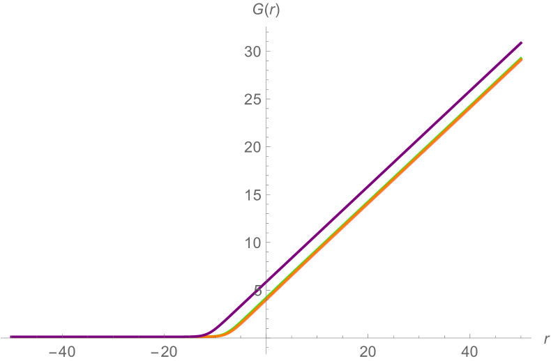
(a) Solution for $G(r)$

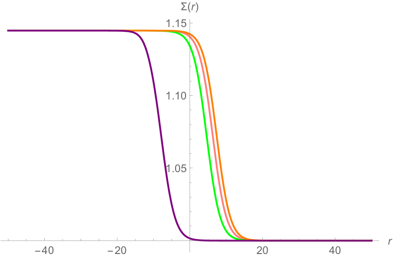
(b) Solution for $\Sigma(r)$

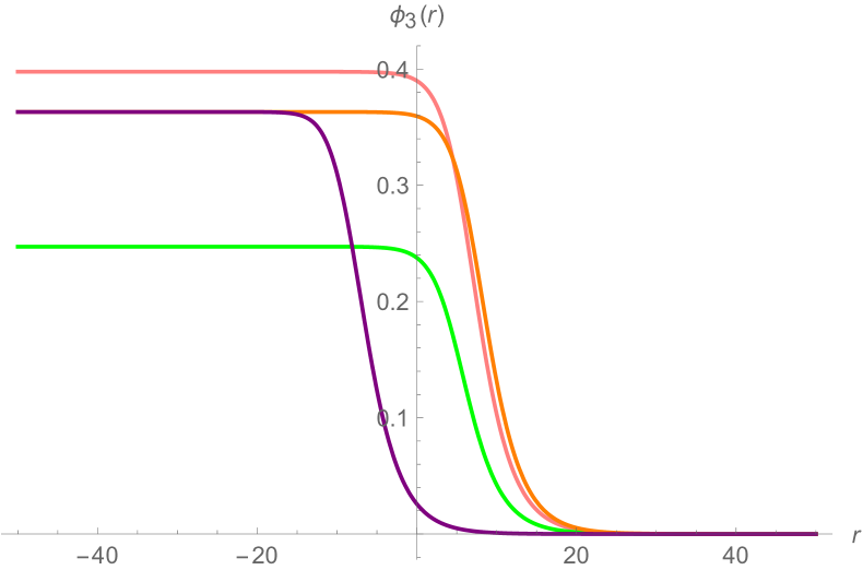
(c) Solution for $\phi_{3}(r)$

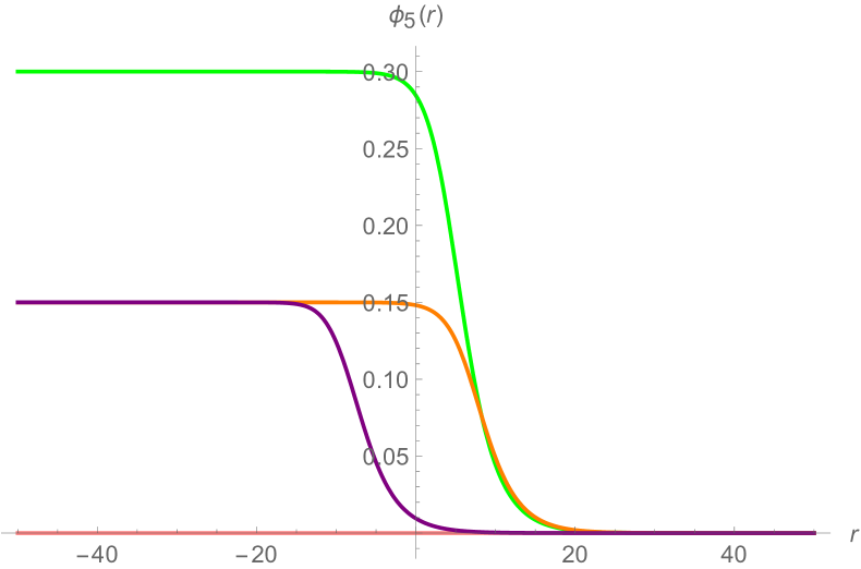
(d) Solution for $\phi_{5}(r)$

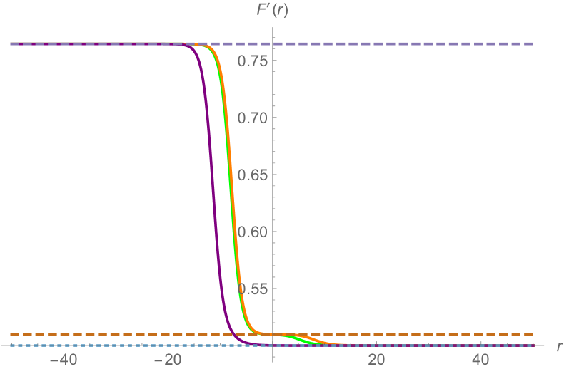
(e) Solution for $F^{\prime}(r)$

Figure 1: Examples of RG flows from $N=4$ and $N=2$ $AdS_{5}$ critical points to $N=(2,0)$ $AdS_{3}\times H^{2}$ fixed point $2$ with $SO(2)_{\textrm{diag}}\times SO(2)$ symmetry in the IR with $\phi_{1}=0$, $a_{6}=0$, $h_{1}=1$, $\rho=\frac{3}{2}$ and $\zeta=\frac{1}{2}$ for $\phi^{*}_{5}=0$ (pink), $\phi^{*}_{5}=0.15$ (orange and purple) and $\phi^{*}_{5}=0.30$ (green).

We now consider solutions flowing to $AdS_{3}\times H^{2}$ critical point $1$ with only $\phi_{1}$ non-vanishing. For $\phi_{3}=\phi_{5}=0$, the truncated BPS equations only admit the $N=4$ $AdS_{5}$ critical point as an asymptotic geometry. Therefore, in this case, there are only solutions interpolating between this $AdS_{5}$ critical point and the $AdS_{3}\times H^{2}$ geometry in the IR. Examples of these solutions for different values of $a_{6}=0.70,0.75,0.80$ are given in figure 2.

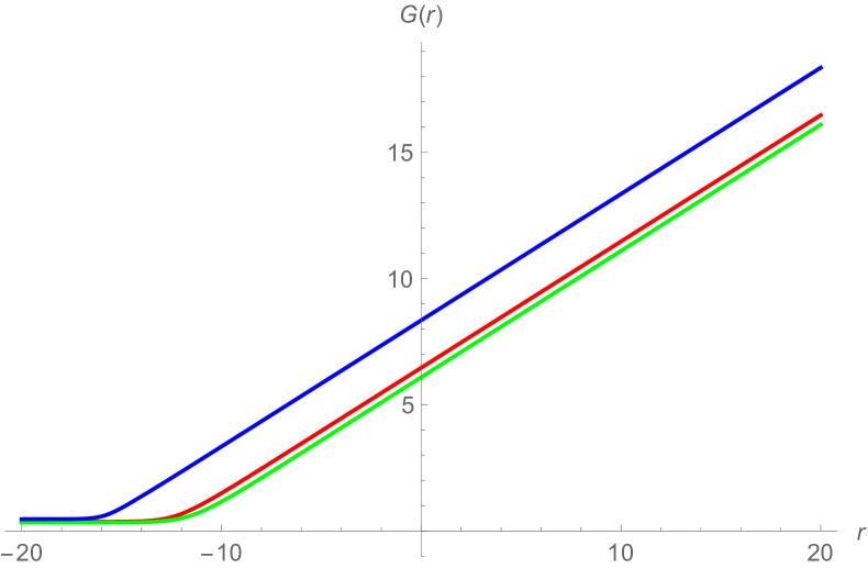
(a) Solution for $G(r)$

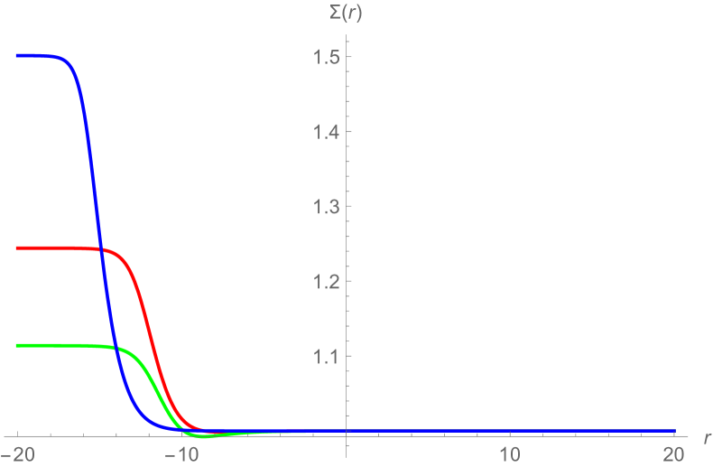
(b) Solution for $\Sigma(r)$

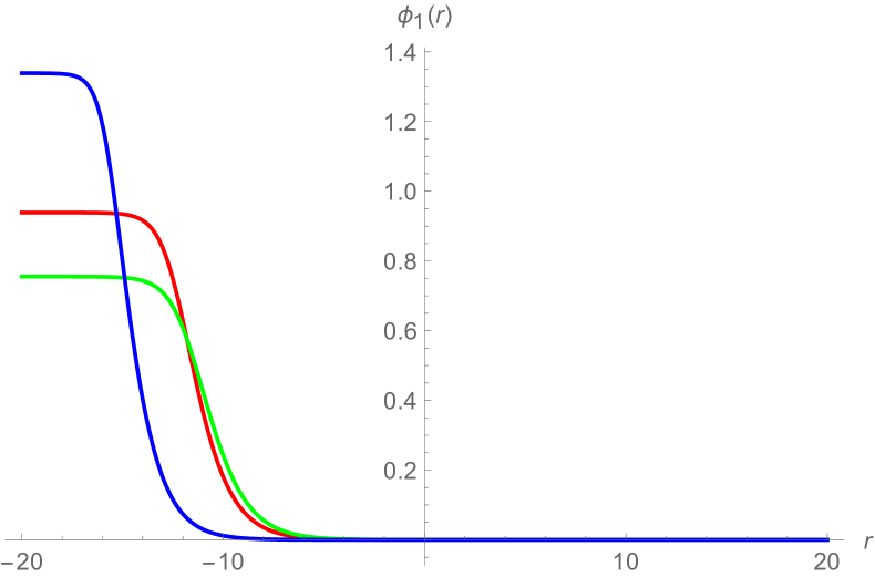
(c) Solution for $\phi_{1}(r)$

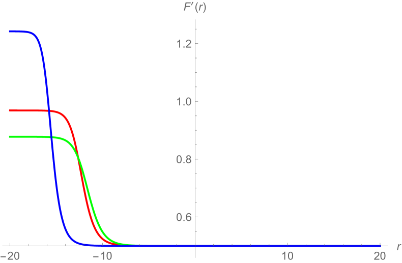
(d) Solution for $F^{\prime}(r)$

Figure 2: Examples of RG flows from $N=4$ $AdS_{5}$ critical point to $N=(2,0)$ $AdS_{3}\times H^{2}$ fixed point $1$ in the IR with $\phi_{3}=\phi_{5}=0$, $h_{1}=1$, $\rho=4$ and $\zeta=\frac{1}{2}$ for $a_{6}=0.70$ (blue), $a_{6}=0.75$ (red) and $a_{6}=0.80$ (green).

Finally, we look for more complicated solutions flowing to $AdS_{3}\times H^{2}$ fixed point $3$ with all scalars non-vanishing. Examples of solutions interpolating between $N=4$ $AdS_{5}$ critical point and this $AdS_{3}\times H^{2}$ fixed point are given in figure 3. It should be noted that at the $AdS_{3}\times H^{2}$ fixed point, only the value of $\phi_{3}$ is affected by the value of $\phi^{*}_{5}$. In addition, the solutions in the figure indicate that apart from the solutions for $\phi_{3}$ and $\phi_{5}$, the entire flow solutions for other fields are not affected by different values of $\phi^{*}_{5}$ at the $AdS_{3}\times H^{2}$ fixed point.

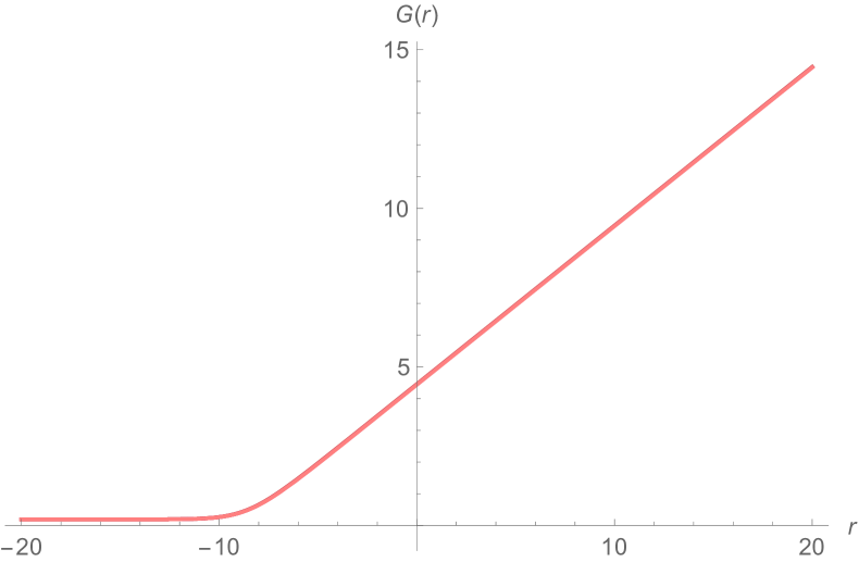
(a) Solution for $G(r)$

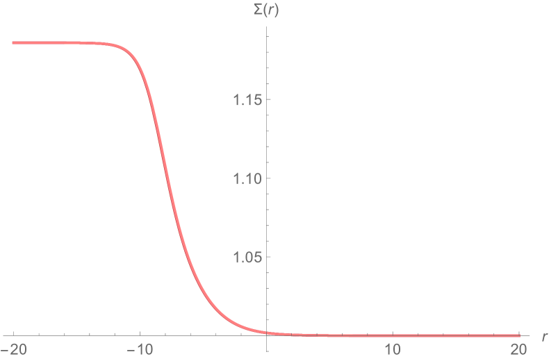
(b) Solution for $\Sigma(r)$

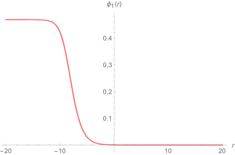
(c) Solution for $\phi_{1}(r)$

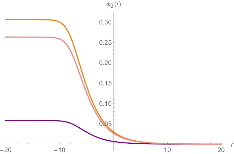
(d) Solution for $\phi_{3}(r)$

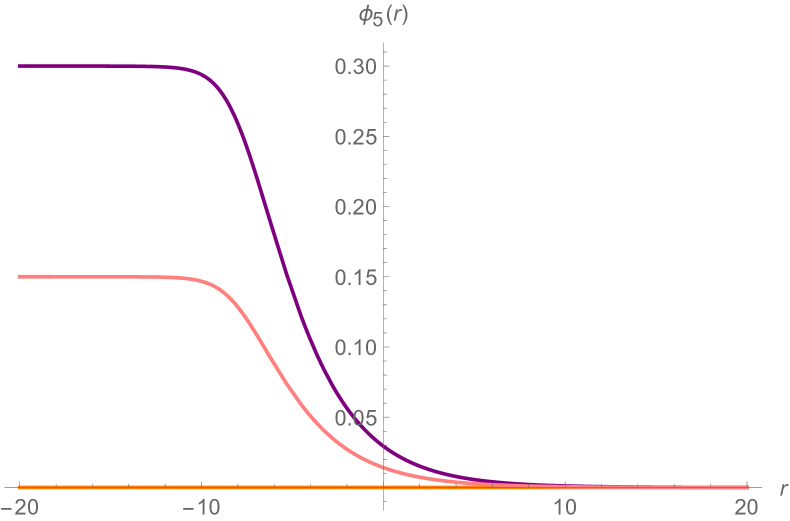
(e) Solution for $\phi_{5}(r)$

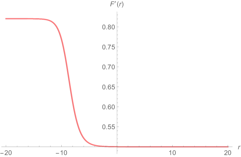
(f) Solution for $F^{\prime}(r)$

Figure 3: Examples of RG flows from $N=4$ $AdS_{5}$ critical point to $N=(2,0)$ $AdS_{3}\times H^{2}$ fixed point $3$ in the IR with $h_{1}=1$, $\rho=\frac{3}{2}$, $\zeta=\frac{1}{2}$ and $a_{6}=\frac{1}{4}$ for $\phi^{*}_{5}=0$ (orange), $\phi^{*}_{5}=0.15$ (pink) and $\phi^{*}_{5}=0.30$ (purple).

All of these solutions describe black strings with a near horizon geometry of the form $AdS_{3}\times H^{2}$ in asymptotically locally $AdS_{5}$ spaces. Holographically, the solutions can also be considered as holographic RG flows from the four-dimensional $N=2$ and $N=1$ SCFTs to two-dimensional $N=(2,0)$ SCFTs in the IR.

4 Supersymmetric $AdS_{5}$ black strings with $SO(2)_{\textrm{diag}}$ symmetry

In this section, we repeat the same analysis for a smaller residual symmetry $SO(2)_{\textrm{diag}}$ that is the diagonal subgroup of $SO(2)_{D}\times SO(2)_{R}\times SO(2)$ generated by $X_{0}$, $X_{3}$ and $X_{6}$. As pointed out in [29], there are nine singlet scalars under $SO(2)_{\textrm{diag}}$ corresponding to the non-compact generators

$$\hat{Y}_{1}=Y_{31},\phantom{-Y_{31}}\qquad\hat{Y}_{2}=Y_{42}+Y_{53},\qquad\hat{Y}_{3}=Y_{44}+Y_{55},$$

$$\hat{Y}_{4}=Y_{43}-Y_{52},\qquad\hat{Y}_{5}=Y_{45}-Y_{54},\qquad\tilde{Y}_{1}=Y_{12}+Y_{23},$$

$$\tilde{Y}_{2}=Y_{13}-Y_{22},\qquad\tilde{Y}_{3}=Y_{14}+Y_{25},\qquad\tilde{Y}_{4}=Y_{15}-Y_{24}\,.$$ (68)

The coset representative is then given by

$$\mathcal{V}=e^{\phi_{1}\hat{Y}_{1}}e^{\phi_{2}\hat{Y}_{2}}e^{\phi_{3}\hat{Y}_{3}}e^{\phi_{4}\hat{Y}_{4}}e^{\phi_{5}\hat{Y}_{5}}e^{\varphi_{1}\tilde{Y}_{1}}e^{\varphi_{2}\tilde{Y}_{2}}e^{\varphi_{3}\tilde{Y}_{3}}e^{\varphi_{4}\tilde{Y}_{4}}\,.$$ (69)

It turns out that the analysis in this case is much more complicated than the previous case of $SO(2)_{\textrm{diag}}\times SO(2)$ symmetry. To proceed further, we will consider a subtruncation of this sector with $\varphi_{1}=\varphi_{2}=\varphi_{3}=\varphi_{4}=0$. However, consistency among the BPS equations and compatibility between the BPS equations and the field equations further require that $\phi_{4}=\phi_{5}=0$. The resulting truncation is accordingly the same as that studied in [29] with only $\phi_{1}$, $\phi_{2}$ and $\phi_{3}$ non-vanishing.
The ansatz for the metric and $(A^{0},A^{3},A^{6})$ gauge fields are the same as in the previous section. To implement the $SO(2)_{\textrm{diag}}$ symmetry, in this case, we impose the following conditions

$$A^{0}=\frac{h_{1}}{g_{2}}A^{3}\qquad\textrm{and}\qquad A^{6}=\frac{h_{1}}{h_{2}}A^{3}\,.$$ (70)

The twist can be performed in the same way as in the previous section with the twist condition (42) and projectors (41) and (43).

4.1 Supersymmetric $AdS_{5}$ vacua

Since the scalar sector considered here is the same as in [29], the $AdS_{5}$ vacua are given by those identified in [29]. We will only give the superpotential and supersymmetric $AdS_{5}$ critical points but refer to [29] for the explicit form of the scalar potential.
The superpotential is given by

$$W = \frac{1}{3}\Sigma^{-1}\cosh^{2}\phi_{3}\left(h_{1}\cosh\phi_{1}\cosh^{2}\phi_{2}+h_{2}\sinh\phi_{1}\sinh^{2}\phi_{2}\right)$$ (71)

$$+\frac{\sqrt{2}}{12}(g_{2}-2g_{1}-g_{2}\cosh 2\phi_{3})\Sigma^{2}$$

which admits the following $AdS_{5}$ critical points:

• I. The trivial critical point, at the origin of $SO(5,5)/SO(5)\times SO(5)$, is given by

  $$\phi_{1}=\phi_{2}=\phi_{3}=0,\qquad\Sigma=-\left(\frac{h_{1}}{\sqrt{2}g_{1}}\right)^{\frac{1}{3}},\qquad V_{0}=-3\left(\frac{g_{1}h_{1}^{2}}{2}\right)^{\frac{2}{3}}\,.$$ (72)

  As in the previous section, this critical point preserves the full $SO(2)_{D}\times SO(3)\times SO(3)$ gauge symmetry and $N=4$ supersymmetry.

• II. Unlike the previous case of $SO(2)_{\textrm{diag}}\times SO(2)$ symmetry, there is another $N=4$ $AdS_{5}$ critical point given by

  $$\phi_{1}=\phi_{2}=\frac{1}{2}\ln\left[\frac{h_{2}-h_{1}}{h_{2}+h_{1}}\right],\qquad\Sigma=-\left(\frac{h_{1}h_{2}}{\sqrt{2}g_{1}\sqrt{h_{2}^{2}-h_{1}^{2}}}\right)^{\frac{1}{3}},$$

  $$\phi_{3}=0,\qquad V_{0}=-\frac{3}{2}\left(\frac{\sqrt{2}g_{1}h_{1}^{2}h_{2}^{2}}{h_{2}^{2}-h_{1}^{2}}\right)^{\frac{2}{3}}\,.$$ (73)

  This critical point preserves $SO(2)_{D}\times SO(3)_{\textrm{diag}}$ symmetry.

• III. The next critical point is given by

  $$\phi_{1}=\phi_{2}=0,\qquad\phi_{3}=\frac{1}{2}\ln\left[\frac{g_{2}-4g_{1}+2\sqrt{4g_{1}^{2}-2g_{1}g_{2}-2g_{2}^{2}}}{3g_{2}}\right],$$

  $$\Sigma=-\left(\frac{\sqrt{2}h_{1}}{g_{2}}\right)^{\frac{1}{3}},\qquad V_{0}=-\frac{1}{3}(g_{1}-g_{2})^{2}\left(\frac{\sqrt{2}h_{1}}{g_{2}}\right)^{\frac{4}{3}}\,.$$ (74)

  This critical point preserves $N=2$ supersymmetry and $SO(2)_{\textrm{diag}}\times SO(3)$ symmetry.

• IV. There is another $N=2$ supersymmetric critical point given by

  $$\phi_{1}=\phi_{2}=\frac{1}{2}\ln\left[\frac{h_{2}-h_{1}}{h_{2}+h_{1}}\right],\qquad\Sigma=\left(\frac{\sqrt{2}h_{1}h_{2}}{g_{2}\sqrt{h_{2}^{2}-h_{1}^{2}}}\right)^{\frac{1}{3}},$$

  $$\phi_{3}=\frac{1}{2}\ln\left[\frac{g_{2}-4g_{1}+2\sqrt{4g_{1}^{2}-2g_{1}g_{2}-2g_{2}^{2}}}{3g_{2}}\right],$$

  $$V_{0}=-\frac{2}{3}(g_{1}-g_{2})^{2}\left(\frac{h_{1}^{2}h_{2}^{2}}{\sqrt{2}g_{2}^{2}(h_{2}^{2}-h_{1}^{2})}\right)^{\frac{2}{3}}$$ (75)

  which is invariant under $SO(2)_{\textrm{diag}}$.

As pointed out in [29], some of these critical points appear in pairs with some sign differences. Since critical points related by these sign changes are physically equivalent, in the above equations, we have chosen a particular sign choice for definiteness.

4.2 Supersymmetric $AdS_{3}\times\Sigma^{2}$ fixed points

With the same anlysis of supersymmetry transformations of fermionic fields, we obtain the BPS equations

$$F^{\prime} = \frac{1}{12g_{2}h_{2}\Sigma^{2}}\left[\sqrt{2}g_{2}h_{2}\Sigma^{4}(g_{2}-2g_{1}-g_{2}\cosh 2\phi_{3})+4g_{2}h_{2}\cosh^{2}\phi_{3}\times\right.$$ (76)

$$(h_{1}\cosh\phi_{1}\cosh^{2}\phi_{2}+h_{2}\sinh\phi_{1}\sinh^{2}\phi_{2})\Sigma$$

$$\left.-2\kappa a_{3}e^{-2G}\left\{2g_{2}\Sigma^{3}(h_{2}\cosh\phi_{1}+h_{1}\sinh\phi_{1})+\sqrt{2}h_{1}h_{2}\right\}\right],$$

$$G^{\prime} = \frac{1}{12g_{2}h_{2}\Sigma^{2}}\left[\sqrt{2}g_{2}h_{2}\Sigma^{4}(g_{2}-2g_{1}-g_{2}\cosh 2\phi_{3})+4g_{2}h_{2}\cosh^{2}\phi_{3}\times\right.$$ (77)

$$(h_{1}\cosh\phi_{1}\cosh^{2}\phi_{2}+h_{2}\sinh\phi_{1}\sinh^{2}\phi_{2})\Sigma$$

$$\left.+4\kappa a_{3}e^{-2G}\left\{2g_{2}\Sigma^{3}(h_{2}\cosh\phi_{1}+h_{1}\sinh\phi_{1})+\sqrt{2}h_{1}h_{2}\right\}\right],$$

$$\Sigma^{\prime} = \frac{1}{3}\cosh^{2}\phi_{3}\left(h_{1}\cosh\phi_{1}\cosh^{2}\phi_{2}+h_{2}\sinh\phi_{1}\sinh^{2}\phi_{2}\right)+\frac{\sqrt{2}}{6}\Sigma^{3}(g_{2}\cosh 2\phi_{3}+2g_{1}$$ (78)

$$-g_{2})+\frac{1}{3g_{2}h_{2}\Sigma}\kappa a_{3}e^{-2G}\left[\sqrt{2}h_{1}h_{2}-2g_{2}\Sigma^{3}(h_{2}\cosh\phi_{1}+h_{1}\sinh\phi_{1})\right],$$

$$\phi_{1}^{\prime} = -\Sigma^{-1}\cosh^{2}\phi_{3}\left(h_{1}\cosh^{2}\phi_{2}\sinh\phi_{1}+h_{2}\cosh\phi_{1}\sinh^{2}\phi_{2}\right)$$ (79)

$$-\frac{\kappa a_{3}}{h_{2}}e^{-2G}\Sigma(h_{1}\cosh\phi_{1}+h_{2}\sinh\phi_{1}),$$

$$\phi_{2}^{\prime} = -\Sigma^{-1}\cosh\phi_{2}\sinh\phi_{2}(h_{1}\cosh\phi_{1}+h_{2}\sinh\phi_{1}),$$ (80)

$$\phi_{3}^{\prime} = \frac{1}{4}\Sigma^{-1}\sinh 2\phi_{3}\left[\sqrt{2}g_{2}\Sigma^{3}-2h_{1}\cosh\phi_{1}\cosh^{2}\phi_{2}-2h_{2}\sinh\phi_{1}\sinh^{2}\phi_{2}\right].$$ (81)

From these equations, we find the following $AdS_{3}\times\Sigma^{2}$ fixed points:

$$i : \quad\phi_{2}=\phi_{3}=0,\quad\phi_{1}=\frac{1}{2}\ln\left[\frac{(h_{2}-h_{1})(g_{1}h_{2}-g_{2}h_{1})}{(h_{2}+h_{1})(g_{2}h_{1}+g_{1}h_{2})}\right],\qquad\qquad\qquad$$ (82)

$$\quad\Sigma=\left(-\frac{\sqrt{2}(g_{1}+g_{2})h_{1}h_{2}^{2}}{g_{2}\sqrt{(h_{2}^{2}-h_{1}^{2})(g_{1}^{2}h_{2}^{2}-g_{2}^{2}h_{1}^{2})}}\right)^{\frac{1}{3}},$$

$$\quad G=\frac{1}{2}\ln\left[\frac{2^{\frac{1}{3}}\kappa a_{3}(g_{1}+g_{2})h_{1}h_{2}^{2}}{g_{2}(g_{2}^{2}h_{1}^{2}-g_{1}^{2}h_{2}^{2})}\right],$$

$$\quad L_{AdS_{3}}=\left(\frac{8\sqrt{2}g_{2}^{2}h_{2}^{2}(g_{1}+g_{2})(h_{2}^{2}-h_{1}^{2})(g^{2}_{2}h_{1}^{2}-g_{1}^{2}h_{2}^{2})}{h_{1}^{2}[g_{2}^{2}h_{1}^{2}+g_{1}^{2}h_{2}^{2}(g_{1}+2g_{2})]^{3}}\right)^{\frac{1}{3}},$$

$$ii : \quad\phi_{3}=0,\quad\phi_{1}=\phi_{2}=\frac{1}{2}\ln\left[\frac{h_{2}-h_{1}}{h_{2}+h_{1}}\right],\quad\Sigma=\left(-\frac{\sqrt{2}h_{1}h_{2}(g_{1}+g_{2})}{g_{1}g_{2}\sqrt{h_{2}^{2}-h_{1}^{2}}}\right)^{\frac{1}{3}},$$ (83)

$$\quad G=\frac{1}{6}\ln\left[-\frac{2g_{2}\kappa a_{3}^{3}(h_{2}^{2}-h_{1}^{2})^{2}}{g_{1}^{2}h_{1}h_{2}^{4}(g_{1}+g_{2})}\right],$$

$$\quad L_{AdS_{3}}=\left(-\frac{8\sqrt{2}g_{2}^{2}(g_{1}+g_{2})(h_{2}^{2}-h_{1}^{2})}{g_{1}h_{1}^{2}h_{2}^{2}(g_{1}+2g_{2})^{3}}\right)^{\frac{1}{3}},$$

$$iii : \quad\phi_{2}=0,\quad\phi_{1}=\frac{1}{2}\ln\left[\frac{h_{2}+h_{1}}{h_{2}-h_{1}}\right],\quad\Sigma=\left(\frac{\sqrt{2}h_{1}h_{2}}{g_{2}\sqrt{h_{2}^{2}-h_{1}^{2}}}\right)^{\frac{1}{3}},$$ (84)

$$\quad\phi_{3}=\frac{1}{2}\ln\left[\frac{g_{2}(h_{2}^{2}-h_{1}^{2})-4g_{1}h_{2}^{2}+2h_{2}\sqrt{2(g_{1}-g_{2})[g_{2}h_{1}^{2}+h_{2}^{2}(2g_{1}+g_{2})]}}{g_{2}(h_{1}^{2}+3h_{2}^{2})}\right],$$

$$\quad G=\frac{1}{6}\ln\left[\frac{2\kappa a_{3}^{3}g_{2}(h_{1}^{2}+3h_{2}^{2})^{3}}{h_{1}h_{2}^{4}(g_{1}-g_{2})^{3}(h_{2}^{2}-h_{1}^{2})}\right],$$

$$\quad L_{AdS_{3}}=\frac{6}{g_{2}-g_{1}}\left(1+\sqrt{\frac{4h_{2}^{2}}{h_{2}^{2}-h_{1}^{2}}}\right)^{-1}\left(\frac{\sqrt{2}g_{2}^{2}(h_{2}^{2}-h_{1}^{2})}{h_{1}^{2}h_{2}^{2}}\right)^{\frac{1}{3}},$$

$$iv : \quad\phi_{1}=\phi_{2}=\frac{1}{2}\ln\left[\frac{h_{2}-h_{1}}{h_{2}+h_{1}}\right],\quad\Sigma=\left(\frac{\sqrt{2}h_{1}h_{2}}{g_{2}\sqrt{h_{2}^{2}-h_{1}^{2}}}\right)^{\frac{1}{3}},\quad\qquad\qquad\qquad$$ (85)

$$\quad\phi_{3}=\frac{1}{2}\ln\left[\frac{g_{2}-4g_{1}+2\sqrt{4g_{1}^{2}-2g_{1}g_{2}-2g_{2}^{2}}}{3g_{2}}\right],$$

$$\quad G=\frac{1}{6}\ln\left[\frac{54\kappa a_{3}^{3}g_{2}(h_{2}^{2}-h_{1}^{2})^{2}}{(g_{1}-g_{2})^{3}h_{1}h_{2}^{4}}\right],$$

$$\quad L_{AdS_{3}}=\frac{2}{g_{2}-g_{1}}\left(\frac{\sqrt{2}g_{2}^{2}(h_{2}^{2}-h_{1}^{2})}{h_{1}^{2}h_{2}^{2}}\right)^{\frac{1}{3}}\,.$$

Among these fixed points, only $ii$ leads to $AdS_{3}\times S^{2}$ geometry. All the remaining fixed points correspond to $AdS_{3}\times H^{2}$ solutions.

4.3 Supersymmetric black string solutions

We now look for supersymmetric black string solutions interpolating between $AdS_{5}$ and $AdS_{3}\times\Sigma^{2}$ geometries. We begin with solutions flowing to $AdS_{3}\times H^{2}$ critical point $i$. With $\phi_{2}=\phi_{3}=0$ and $\kappa=-1$, examples of solutions interpolating between $N=4$ $AdS_{5}$ critical point I and $AdS_{3}\times H^{2}$ fixed point $i$ are shown in figure 4.

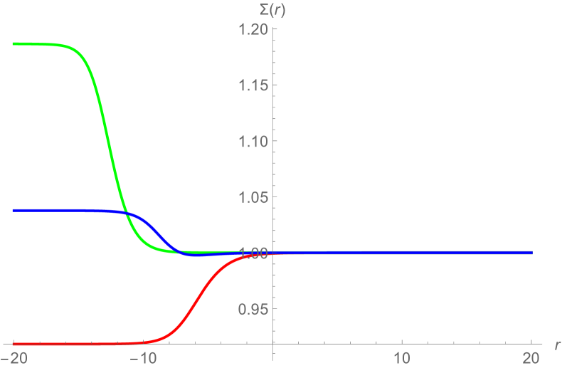
(a) Solution for $\Sigma(r)$

(b) Solution for $\phi_{1}(r)$

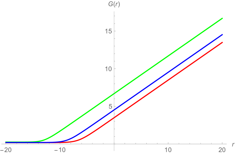
(c) Solution for $G(r)$

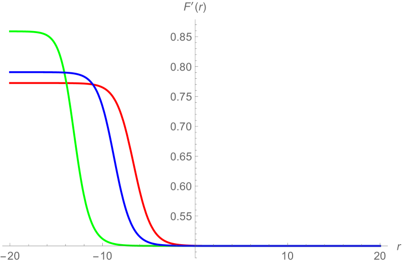
(d) Solution for $F^{\prime}(r)$

Figure 4: RG flows from $N=4$ $AdS_{5}$ critical point I to $N=(2,0)$ $AdS_{3}\times H^{2}$ fixed point $i$ with $\phi_{2}=\phi_{3}=0$, $h_{1}=1$, $\zeta=\frac{1}{2}$ for $\rho=1.20$ (green), $\rho=1.35$ (blue), $\rho=1.50$ (red).

We now move to solutions involving $AdS_{3}\times\Sigma^{2}$ fixed point $ii$. Unlike other cases, the solutions in this case only exist for $\kappa=1$. Some examples of solutions for $\phi_{3}=0$ are given in figure 5. There is a solution flowing directly from $N=4$ $AdS_{5}$ vacuum I to $AdS_{3}\times S^{2}$ fixed point $ii$ (red line). There are also solutions that flow to $AdS_{3}\times S^{2}$ fixed point $ii$ and approach arbitrarily close to $N=4$ $AdS_{5}$ critical point II shown by green, purple and blue lines. Similarly, setting $\phi_{2}=0$, we find solutions interpolating between $AdS_{5}$ critical point I and $AdS_{3}\times H^{2}$ fixed point $iii$ with some examples of these solutions shown in figure 6.

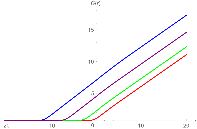
(a) Solution for $G(r)$

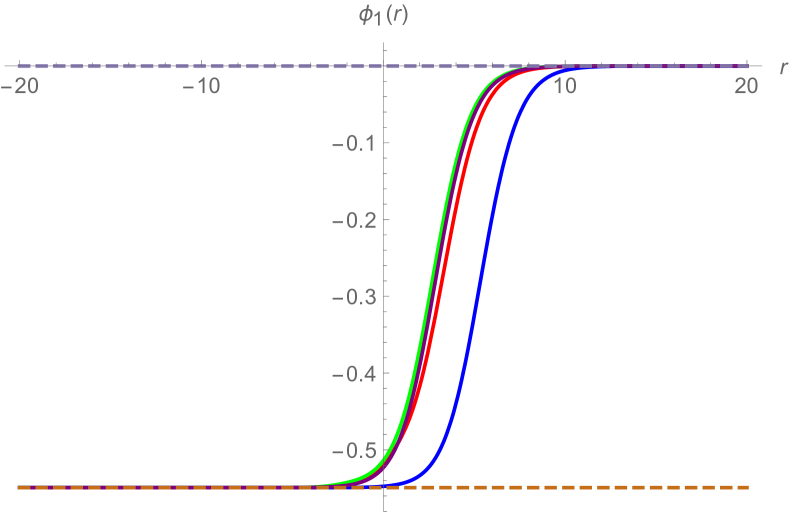
(b) Solution for $\phi_{1}(r)$

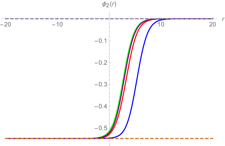
(c) Solution for $\phi_{2}(r)$

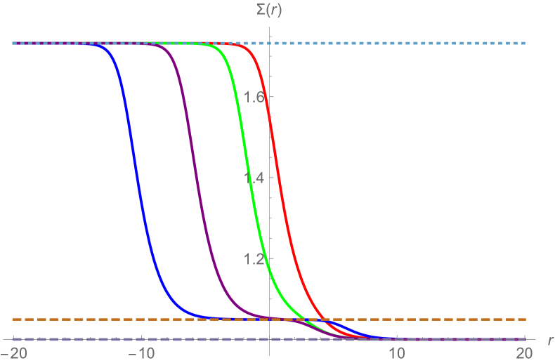
(d) Solution for $\Sigma(r)$

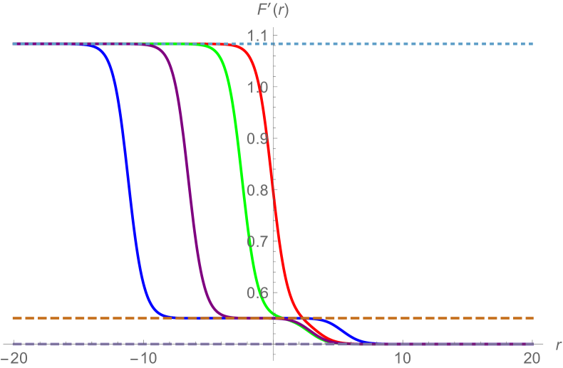
(e) Solution for $F^{\prime}(r)$

Figure 5: RG flows from $N=4$ $AdS_{5}$ critical points I and II to $N=(2,0)$ $AdS_{3}\times S^{2}$ fixed point $ii$ in the IR with $\phi_{3}=0$, $h_{1}=1$, $\rho=-\frac{5}{2}$ and $\zeta=\frac{1}{2}$.

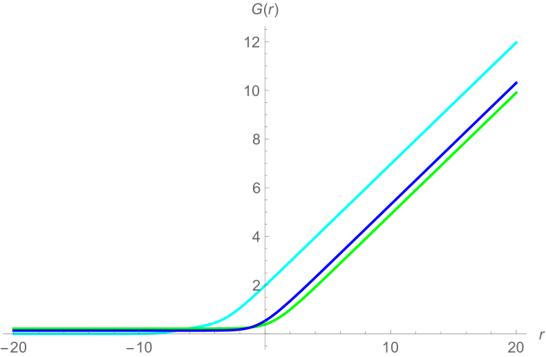
(a) Solution for $G(r)$

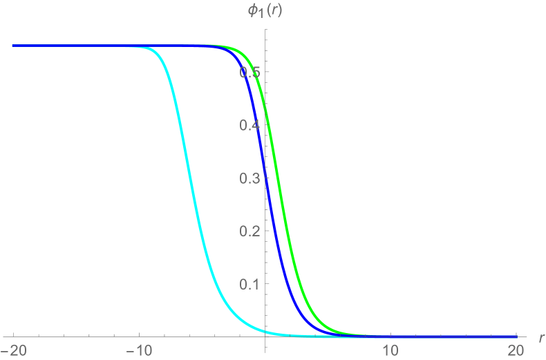
(b) Solution for $\phi_{1}(r)$

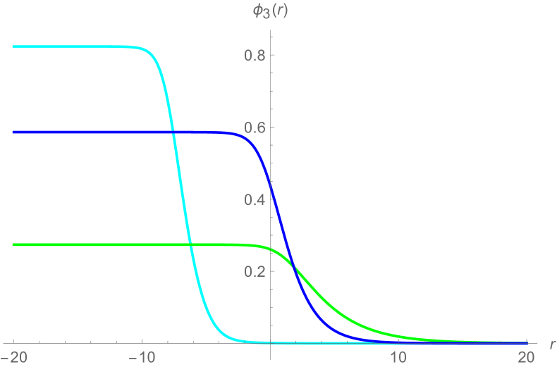
(c) Solution for $\phi_{3}(r)$

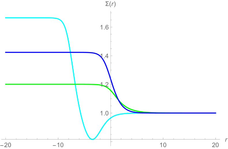
(d) Solution for $\Sigma(r)$

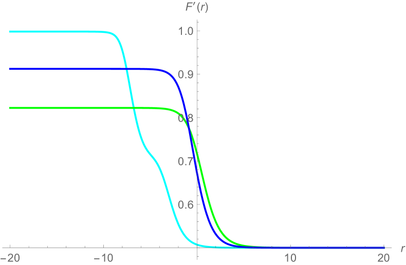
(e) Solution for $F^{\prime}(r)$

Figure 6: RG flows from $N=4$ $AdS_{5}$ critical point I to $N=(2,0)$ $AdS_{3}\times H^{2}$ fixed point $iii$ in the IR with $\phi_{2}=0$, $h_{1}=1$, $\zeta=\frac{1}{2}$ and $\rho=\frac{3}{2}$ (green), $\rho=\frac{5}{2}$ (blue), $\rho=4$ (cyan).

Finally, we consider solutions that flow to $AdS_{3}\times H^{2}$ critical point $iv$. We first note that the values of scalar fields are the same as those for $N=2$ $AdS_{5}$ critical point IV. By setting all scalar fields to the values at these critical points, we find a solution involving only $F(r)$ and $G(r)$ given by

$$G = \frac{1}{2}\ln\left[\frac{e^{\frac{2(r-r_{0})}{L_{5}}}+6a_{3}g_{2}^{\frac{1}{3}}(h_{2}^{2}-h_{1}^{2})}{h_{2}(g_{2}-g_{1})[4h_{1}h_{2}(h_{2}^{2}-h_{1}^{2})]^{\frac{1}{3}}}\right],\quad L_{5}=\frac{3}{(g_{2}-g_{1})}\left(\frac{g_{2}^{2}(h_{2}^{2}-h_{1}^{2})}{4\sqrt{2}h_{1}^{2}h_{2}^{2}}\right)^{\frac{1}{3}},$$

$$F = \frac{3r}{2L_{5}}-\frac{1}{4}\ln\left[e^{\frac{2(r-r_{0})}{L_{5}}}+6a_{3}g_{2}^{\frac{1}{3}}(h_{2}^{2}-h_{1}^{2})\right].$$ (86)

For more general solutions with scalars depending on $r$, we can find only numerical solutions. Examples of these solutions can be found in figure 7. In this case, the solutions are more interesting than those of the previous cases. There is a solution interpolating between $AdS_{5}$ critical point I to $AdS_{3}\times H^{2}$ fixed point $iv$ shown by the purple line. On the other hand, there are solutions interpolating among $AdS_{5}$ critical points I, II and IV and $AdS_{3}\times H^{2}$ fixed point $iv$. Some of these solutions connects all these critical points within a single flow (pink line). There are also solutions interpolating between two $AdS_{5}$ vacua and $AdS_{3}\times H^{2}$ fixed point $iv$ as shown by the orange and cyan lines. The former begins at critical point I and flows to critical points IV and $iv$ while the latter flows from critical point I to critical points II and $iv$.
As in the previous section, these solutions should also holographically describe various possible RG flows from $N=2$ and $N=1$ SCFTs in four dimensions to $N=(2,0)$ two-dimensional conformal fixed points in the IR.

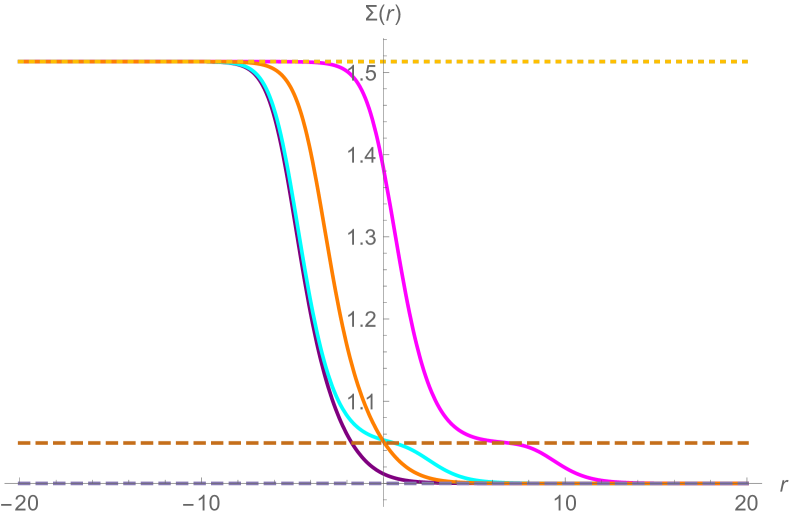
(a) Solution for $\Sigma(r)$

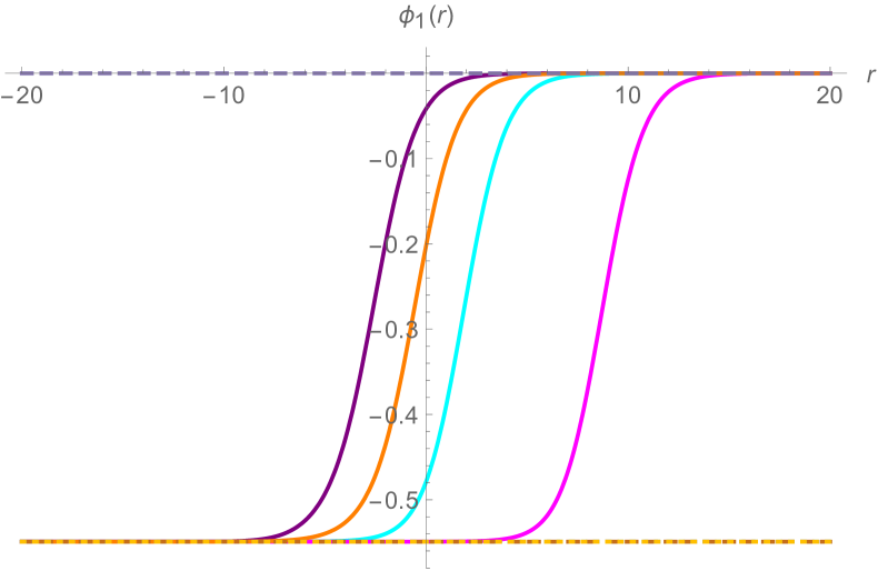
(b) Solution for $\phi_{1}(r)$

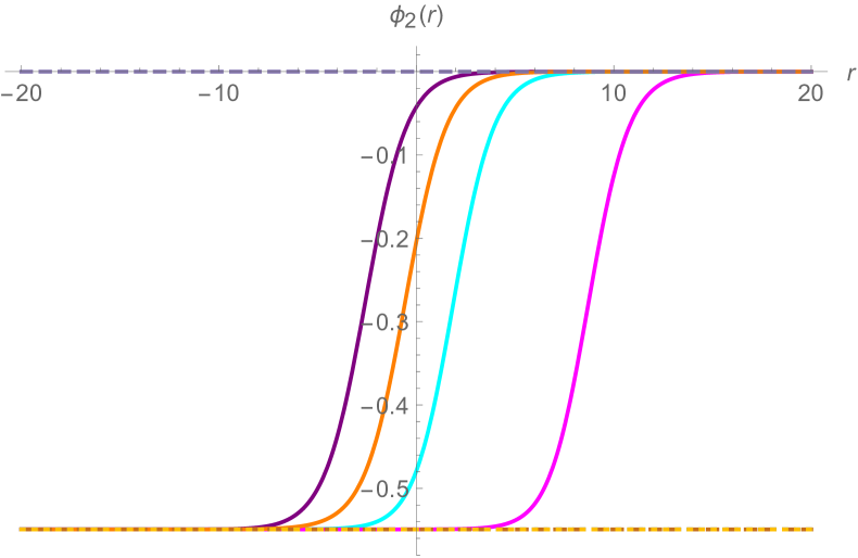
(c) Solution for $\phi_{2}(r)$

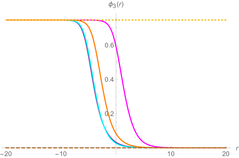
(d) Solution for $\phi_{3}(r)$

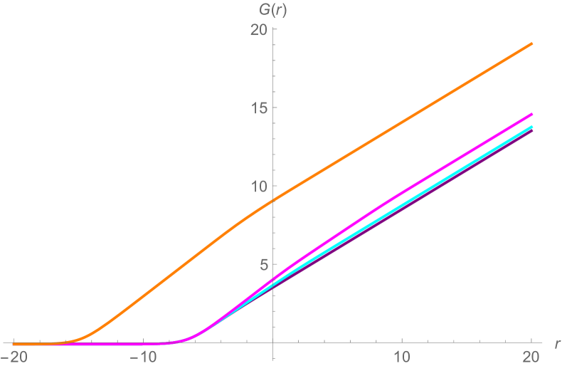
(e) Solution for $G(r)$

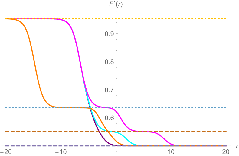
(f) Solution for $F^{\prime}(r)$

Figure 7: RG flows from $AdS_{5}$ critical points I, II and IV to $N=(2,0)$ $AdS_{3}\times H^{2}$ fixed point $iv$ with $h_{1}=1$, $\zeta=\frac{1}{2}$ and $\rho=3$.

5 Conclusions and discussions

In this paper, we have constructed a large number of supersymmetric $AdS_{5}$ black string solutions from five-dimensional $N=4$ gauged supergravity with $SO(2)_{D}\times SO(3)\times SO(3)$ gauge group. The solutions interpolate between a number of different $AdS_{5}$ and $AdS_{3}\times\Sigma^{2}$ critical points and preserve $SO(2)_{\textrm{diag}}\times SO(2)$ or $SO(2)_{\textrm{diag}}$ symmetry and two supercharges. On the other hand, the $AdS_{3}\times\Sigma^{2}$ fixed points preserve $4$ supercharges corresponding to $N=(2,0)$ or $N=(0,2)$ superconformal symmetry in two dimensions. Some of the solutions can even be analytically obtained. Although most of the solutions describe black strings with $AdS_{3}\times H^{2}$ near horizon geometry, we have also found one $AdS_{3}\times S^{2}$ solution with $SO(2)_{\textrm{diag}}$ symmetry. The solutions could be of interest in microscopic counting of black string entropy along the line of [11, 12, 13, 14]. Holographically, the solutions also describe various RG flows from four-dimensional $N=1$ and $N=2$ SCFTs to two-dimensional $N=(2,0)$ SCFTs in the IR via twisted compactifications on $\Sigma^{2}$. The solutions given here are expected to be useful in holographic study of strongly coupled $N=1,2$ SCFTs in four dimensions with topological twists as well.
It should be pointed out that the $N=2$ $AdS_{5}$ vacuum with $SO(2)_{\textrm{diag}}\times SO(3)$ symmetry, obtained from $SO(2)_{\textrm{diag}}\times SO(2)$ sector, together with $AdS_{3}\times H^{2}$ fixed point $2$ and related flow solutions can be embedded in $N=4$ gauged supergravity with $n=2,3$ vector multiplets. The latter can be obtained from the gauged supergravity considered here by truncating out $\phi_{1}$ and the gauge field $A^{6}_{\mu}$ resulting in $N=4$ gauged supergravity with $SO(2)_{D}\times SO(3)_{R}$ gauge group. It has been shown in [37] that this gauged supergravity can be embedded in eleven dimensions.Therefore, within the above truncation, the solutions given here can be uplifted to M-theory. It is then of particular interest to construct the truncation ansatz from the result of [37] and uplift the black string solutions found here to M-theory. This would lead to a new holographic dual of $N=(2,0)$ SCFTs in two dimensions within string/M-theory context.
Moreover, it could be interesting to identify the $N=1$ and $N=2$ SCFTs dual to the $AdS_{5}$ vacua and the two-dimensional conformal fixed points in the IR as well as the associated RG flows in the field theory context. Partial results along this direction have been given in [41] in which the possible dual $N=1$ and $N=2$ SCFTs have been identified. It would be useful to extend these results to the case with topological twists. Furthermore, constructing similar solutions in the form of $AdS_{3}\times\mathbb{\Sigma}$ with $\mathbb{\Sigma}$ being a spindle or a half-spindle along the line of recent results in [42, 43, 44, 45] is also worth considering. Finally, finding similar solutions within $N=4$ gauged supergravity with gauge groups identified in [37] as embeddable in eleven dimensions would lead to new holographic solutions in string/M-theory framework. We leave all these and related issues for future work.
Acknowledgement
This work is funded by National Research Council of Thailand (NRCT) and Chulalongkorn University under grant N42A650263.

References

- [1] F. Benini, K. Hristov and A. Zaffaroni, “Black hole microstates in from supersymmetric localization”, JHEP 05 (2016) 054, arXiv: 1511.04085.
- [2] S. M. Hosseini and A. Zaffaroni, “Large matrix models for 3d theories: twisted index, free energy and black holes”, JHEP 08 (2016) 064, arXiv: 1604.03122.
- [3] F. Benini, K. Hristov and A. Zaffaroni, “Exact microstate counting for dyonic black holes in ”, Phys. Lett. B771 (2017) 462–466, arXiv: 1608.07294.
- [4] S. M. Hosseino, A. Nedelin and A. Zaffaroni, “The Cardy limit of the topologically twisted index and black strings in ”, JHEP 04 (2017) 014, arXiv: 1611.09374.
- [5] F. Azzurli, N. Bobev, P. M. Crichigno, V. S. Min and A. Zaffaroni, “A universal counting of black hole microstates in ”, JHEP 02 (2018) 054, arXiv: 1707.04257.
- [6] S. M. Hosseini, K. Hristov and A. Passias, “Holographic microstate counting for black holes in massive IIA supergravity”, JHEP 10 (2017) 190, arXiv: 1707.06884.
- [7] F. Benini, H. Khachatryan and P. Milan, “Black hole entropy in massive Type IIA”, Class. Quant. Grav. 35 no. 3, (2018) 035004, arXiv: 1707.06886.
- [8] N. Bobev, V. S. Min and K. Pilch, “Mass-deformed ABJM and black holes in ”, JHEP 03 (2018) 050, arXiv: 1801.03135.
- [9] A. Cabo-Bizet, V. I. Giraldo-Rivera, and L. A. Pando Zayas, “Microstate counting of hyperbolic black hole entropy via the topologically twisted index”, JHEP 08 (2017) 023, arXiv: 1701.07893.
- [10] A. Zaffaroni, “Lectures on AdS Black Holes, Holography and Localization”, arXiv: 1902.07176.
- [11] S. M. Hosseini, A. Nedelin, A. Zaffaroni, “The Cardy limit of the topologically twisted index and black strings in ”, JHEP 04 (2017) 014, arXiv: 1611.09374.
- [12] J. Hong and J. T. Liu, “The topologically twisted index of super-Yang-Mills on and the elliptic genus”, JHEP 07 (2018) 018, arXiv: 1804.04592.
- [13] S. M. Hosseini, K. Hristov, A. Zaffaroni, “Microstates of rotating strings”, JHEP 11 (2019) 090, arXiv: 1909.08000.
- [14] S. M. Hosseini, K. Hristov, Y. Tachikawa, A. Zaffaroni, “Anomalies, Black strings and the charged Cardy formula”, JHEP 09 (2020) 167, arXiv: 2006.08629.
- [15] J. Maldacena and C. Nunez, “Supergravity description of field theories on curved manifolds and a no go theorem”, Int. J. Mod. Phys. A16 (2001) 822, arXiv: hep-th/0007018.
- [16] D. Klemm and W. A. Sabra, “Supersymmetry of black strings in gauged supergravities”, Phys. Rev. D62 (2000) 024003, arXiv: hep-th/0001131.
- [17] S. L. Cacciatori, D. Klemm and W. A. Sabra, “Supersymmetric domain walls and strings in gauged supergravity coupled to vector multiplets”, JHEP 03 (2003) 023, arXiv: hep-th/0302218.
- [18] A. Bernamonti, M. M. Caldarelli, D. Klemm, R. Olea, C. Sieg and E. Zorzan, “Black strings in ”, JHEP 01 (2008) 061, arXiv: 0708.2402.
- [19] F. Benini and N. Bobev, “Two-dimensional SCFTs from wrapped branes and c-extremization”, JHEP 06 (2013) 005, arXiv: 1302.4451.
- [20] P. Karndumri and E. O Colgain, “3D Supergravity from wrapped D3-branes”, JHEP 10 (2013) 094, arXiv: 1307.2086.
- [21] N. Bobev, K. Pilch, and O. Vasilakis, “ SCFTs from the Leigh-Strassler fixed point”, JHEP 06 (2014) 094, arXiv:1403.7131.
- [22] F. Benini, N. Bobev and P. M. Crichigno, “Two-dimensional SCFTs from D3-branes”, JHEP 07 (2016) 020, arXiv: 1511.09462.
- [23] D. Klemm, N. Petri and M. Rabbiosi, “Black string first order flow in , abelian gauged supergravity”, JHEP 01 (2017) 106, arXiv: 1610.07367.
- [24] N. Bobev and P. M. Crichigno, “Universal RG Flows Across Dimensions and Holography”, JHEP 12 (2017) 065, arXiv: 1708.05052.
- [25] M. Azzola, D. Klemm and M. Rabbiosi, “ black strings in the stu model of FI-gauged supergravity”, JHEP 10 (2018) 080, arXiv: 1803.03570.
- [26] A. Amariti and C. Toldo, “Betti multiplets, flows across dimensions and c-extremization”, JHEP 07 (2017) 040, arXiv: 1610.08858.
- [27] H. L. Dao and P. Karndumri, “Holographic RG flows and black strings from 5D half-maximal gauged supergravity”, Eur. Phys. J. C79 (2019) 137, arXiv: 1811.01608.
- [28] H. L. Dao and P. Karndumri, “Holographic RG flows and black strings from 5D half-maximal gauged supergravity”, Eur. Phys. J. C79 (2019) 247, arXiv: 1812.10122.
- [29] P. Karndumri, “ vacua and holographic RG flows from 5D gauged supergravity”, Eur. Phys. J. C83 (2023) 164, arXiv: 2209.05270.
- [30] J. P. Gauntlett, N. Kim, and D. Waldram, “M five-branes Wrapped on Supersymmetric Cycles”, Phys. Rev. D63 (2001) 126001, arXiv: hep-th/0012195.
- [31] J. P. Gauntlett and N. Kim, “M five-branes wrapped on supersymmetric cycles II”, Phys. Rev. D65 (2002) 086003, arXiv: hep-th/0109039.
- [32] F. Benini and N. Bobev, “Two-dimensional SCFTs from wrapped branes and c-extremization”, JHEP 06 (2013) 005, arXiv: 1302.4451.
- [33] P. Karndumri and E. O Colgain, “3D Supergravity from wrapped D3-branes”, JHEP 10 (2013) 094, arXiv: 1307.2086.
- [34] P. Karndumri and E. O Colgain, “3D Supergravity from wrapped M5-branes”, JHEP 03 (2016) 188, arXiv: 1508.00963.
- [35] P. Karndumri, “Twisted compactification of 5D SCFTs to three and two dimensions from gauged supergravity”, JHEP 09 (2015) 034, arXiv: 1507.01515.
- [36] P. Karndumri and P. Nuchino, “Two-dimensional SCFTs from matter-coupled gauged supergravity”, Eur. Phys. J. C79 (2019) 652, arXiv: 1905.13085.
- [37] E. Malek and V. V. Camell, “Consistent truncations around half-maximal vacua of -dimensional supergravity”, Class. Quant. Grav. 39 (2022) 7, 075026, arXiv: 2012.15601.
- [38] J. Schon and M. Weidner, “Gauged supergravities”, JHEP 05 (2006) 034, arXiv: hep-th/0602024.
- [39] G. Dall’Agata, C. Herrmann, and M. Zagermann, “General matter coupled gauged supergravity in five-dimensions”, Nucl. Phys. B612 (2001) 123–150, arXiv: hep-th/0103106.
- [40] J. Louis, H. Triendl and M. Zagermann, “ supersymmetric vacua and their moduli spaces”, JHEP 10 (2015) 083, arXiv:1507.01623.
- [41] N. Bobev, D. Cassani and H. Triendl, “Holographic RG Flows for Four-dimensional SCFTs”, JHEP 06(2018)086, arXiv: 1804.03276.
- [42] P. Ferrero, J. P. Gauntlett, J. M. Perez Ipina, D. Martelli and J. Sparks, “D3-Branes Wrapped on a Spindle”, Phys. Rev. Lett. 126 (2021) 111601, arXiv: 2011.10579.
- [43] P. Ferrero, J. P. Gauntlett and J. Sparks, “Supersymmetric spindles”, JHEP 01 (2022) 102, arXiv: 2112.01543.
- [44] S. M. Hosseini, K. Hristov and A. Zaffaroni, “Rotating multi-charge spindles and their microstates”, JHEP 07 (2021) 182, arXiv: 2104.11249.
- [45] A. Boido, J. M. P. Ipina and J. Sparks, “Twisted D3-brane and M5-brane compactifications from multi-charge spindles”, JHEP 07 (2021) 222, arXiv: 2104.13287.