Additive Covariance Matrix Models: Modelling Regional Electricity Net-Demand in Great Britain

Abstract

Forecasts of regional electricity net-demand, consumption minus embedded generation, are an essential input for reliable and economic power system operation, and energy trading. While such forecasts are typically performed region by region, operations such as managing power flows require spatially coherent joint forecasts, which account for cross-regional dependencies. Here, we forecast the joint distribution of net-demand across the 14 regions constituting Great Britain’s electricity network. Joint modelling is complicated by the fact that the net-demand variability within each region, and the dependencies between regions, vary with temporal, socio-economical and weather-related factors. We accommodate for these characteristics by proposing a multivariate Gaussian model based on a modified Cholesky parametrisation, which allows us to model each unconstrained parameter via an additive model. Given that the number of model parameters and covariates is large, we adopt a semi-automated approach to model selection, based on gradient boosting. In addition to comparing the forecasting performance of several versions of the proposed model with that of two non-Gaussian copula-based models, we visually explore the model output to interpret how the covariates affect net-demand variability and dependencies.

The code for reproducing the results in this paper is available at https://doi.org/10.5281/zenodo.7315105, while methods for building and fitting multivariate Gaussian additive models are provided by the SCM R package, available at https://github.com/VinGioia90/SCM.

Keywords: Covariance Matrix Regression Modelling; Generalized Additive Models; Modified Cholesky Decomposition; Multivariate Electricity Net-Demand Forecasting.

1 Introduction

Electricity networks are changing from centralised systems, where power is generated by large power plants connected to the transmission network and consumed mostly on the distribution network, to decentralised networks where significant generation and storage is connected directly to distribution networks. The growth of this embedded generation means that the transmission network now needs to serve the net-demand of customers, that is their demand net of local production. In Great Britain (GB), embedded production comes mostly from domestic and small-to-medium commercial solar and wind farms, as well as small thermal power plants. The lack of visibility of these units at the transmission level, combined with the weather-dependent nature of renewable generation leads to considerable challenges in energy trading and power system operation (huxley2022uncertainties).

The purpose of this work is to support such key operations by proposing an interpretable modelling approach that provides probabilistic, spatially coherent short-term net-demand forecasts. The energy industry is conservative by nature due to the need to maintain security of supply (von2006electric, see Chapter 8 of ). As a result, new processes will only be adopted if they are trusted, and interpretability plays an important role in building trust. Further, interpretability is of critical importance when extrapolation is required, for example during exceptional events such as extreme temperatures, or when the model’s predictions must be decomposed into the contribution of several effects.

Predicting power flows on the electricity transmission network is a key motivating application for probabilistic, spatially coherent modelling in energy forecasting. This is important for both network operators, who are responsible for system security, and traders who must be aware of spatial variation in prices. Power flows are influenced by the injection and offtake of power from the network, as well as network configuration. They are also constrained by the physics of the network and must be forecasted to identify and mitigate any risk of exceeding thermal or stability limits. Therefore, spatial probabilistic forecasts of supply and demand are required to forecast power flows, and quantify uncertainty and risk associated with these constraints. Further, as the configuration of the network may change, any forecasting system must be flexible enough to allow the aggregation of supply and demand on the fly to calculate flows across relevant boundaries (tuinema2020probabilistic).

Motivated by the need for probabilistic joint net-demand forecasts, we consider joint modelling of net-demand across the 14 regions constituting GB’s transmission network, which are shown in Figure 1. The net-demand in each region is the aggregate of the net-demand across many Grid Supply Points (GSPs), the latter being the interfaces between the transmission system and either a distribution network or a high-voltage consumer. Correctly modelling the dependency structure between regions is critical as an error in such a structure would pollute downstream predictions of power flows. Further, joint probabilistic forecasts of regional net-demand can be flexibly post-processed to produce forecasts tailored to the needs of different analyses. For example, when sustained winds blow in the North of the country, the boundary between Scotland and the North of England is of particular interest. Indeed, the power flows across this boundary can be substantial, their direction and size being driven mostly by wind generation in Scotland, where embedded wind capacity far exceeds regional demand. Similarly, when the sun shines across the country, power flows from the South of England, where most of the country’s solar generation units are installed, to London and the Midlands. During winter peak hours, the boundaries between London and its surroundings are characterised by heavy power flows directed toward the Capital, driven by high demand and low generation capacity in the city.

While National Grid’s 2021 ten year statement (elect10year) gives a detailed description of tens of transmission grid boundaries and explains under which circumstances the power lines crossing them become heavily loaded, the examples given above are meant to convey the fact that power flow analysis on operational time scales needs regional net-demand forecasts that can be aggregated, or more generally post-processed, to match the particular scenario of interest. For concreteness, in this work we consider the aggregation into the five GSP macro-regions shown in Figure 1, which are motivated by the boundaries mentioned above and match closely the critical boundaries presented in a Regional Trends and Insights report from the National Grid (NG_bound, see Figure 1 therein).

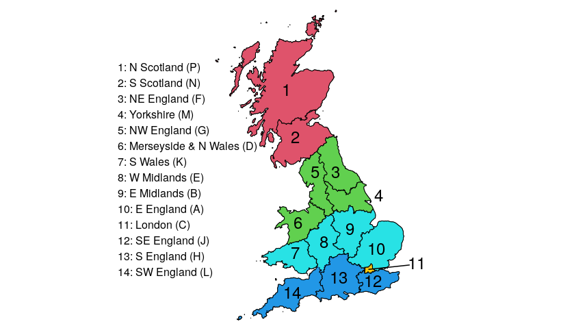
Figure 1: A map of the GSP groups forming GB’s electricity grid. The letters are the designation used by the electricity market in GB, while the numbers correspond to the position of each GSP group in the response vector, $\mathbb{y}_{i}$ (see Section 3.2). The colours represent five macro-regions namely Scotland (red), Northern (green), Midlands (light blue), Southern (blue) and London (yellow). The data on GSPs boundaries is from https://data.nationalgrideso.com.

Forecasts of power flows, which are composite variables of demand and supply, among many other factors, can only be calculated if a multivariate predictive distribution of said quantities is available. Hence, joint forecasts of net-demand across the GSP regions shown in Figure 1, or across an appropriate, scenario-dependent aggregation of them, are essential to help the network operator to take early action when managing the risk of breaching constraints. However, the structure of spatial dependency in net-demand is complex, as it is influenced by both socio-economic and weather effects, and is time-varying. Figure 2a-b illustrates the issue. In particular, the nodes and edges of the network represent, respectively, the conditional regional standard deviations and inter-regional correlations of net-demand, predicted one day ahead by one of the models proposed in this paper. Figure 2a corresponds to New Year’s Eve, a day where net-demand forecast uncertainty is particularly high and correlation is strong between densely populated areas, such as London and the West Midlands. In contrast, Figure 2b corresponds to the 20th of August and shows that net-demand is predicted to lead to a quieter day, from a network management perspective, with weak spatial dependency in forecast uncertainty.

Figure 2: Conditional standard deviations (nodes) and correlations (edges) across the 14 GSP regions (a–b) or macro-regions (c to e), predicted by the model from Section 3.3. The edges corresponding to correlations lower than 0.25 have been made transparent. The plots correspond to 7am on 31/12/18 (a), midnight on 20/08/18 (b) and 10am on 14/06/18 (c to e). Plot d is based on regional wind and precipitation forecasts, while c and e correspond to, respectively, a 25% decrease and increase of such forecasts.

Figure 2a-b makes clear that capturing the time-varying nature of regional net-demand dynamics is essential to produce operationally useful joint forecasts. However, several other factors affect the joint distribution of regional net-demand, in addition to daily and yearly seasonalities. For example, the right column of Figure 2 shows the joint configuration of the macro-regional net-demand variabilities and dependencies during storm Hector. In particular, Figure 2d shows the prediction obtained by conditioning on the seasonal factors and weather forecasts corresponding to this time period. Figures 2c–e have been obtained by respectively decreasing and increasing the regional wind speed and precipitation forecasts by 25%. They show that weather has a strong effect on the joint distribution of net-demand. Specifically, a strengthening of the storm is predicted to lead to a higher variability in Scotland and to stronger correlations between the latter and the other macro-regions.

Having motivated the need for an interpretable covariance matrix modelling framework able to provide the spatially coherent net-demand forecasts required by power flow analysis, we now outline the modelling approach proposed here. We jointly model GB regional net-demand using a multivariate Gaussian model, based on a covariance matrix parametrisation that allows us to model each of its unconstrained parameters via a separate additive model, containing both parametric and smooth spline-based effects. In particular, the covariance matrix of the regional net-demand vector is parametrised via the modified Cholesky decomposition (MCD) of pourahmadi1999. The wiggliness of the smooth effects is controlled via smoothing penalties, the strength of the latter being controlled via smoothing parameters. Model fitting is performed via two nested iterations, the regression coefficients being estimated via maximum a posteriori (MAP) methods, while the smoothing parameters are selected by maximising a Laplace approximation to the marginal likelihood (LAML).

The proposed model can be seen as a multi-parameter generalized additive model (GAM, hastie1987generalized) or as a generalized additive model for location, scale and shape (GAMLSS, rigby2005generalized). Additive models are popular modelling tools in the electricity demand forecasting (see, e.g., fan2011short), in part because they strike a balance between predictive performance and interpretability, the importance of the latter in this context having been discussed above. While ensuring interpretability is challenging under the richly parametrised model considered here, the MCD parametrisation provides some degree of interpretability when the response vector has some, not necessarily unique, intrinsic ordering, as is the case for regional net-demand. We further enhance interpretable exploration of the model by summarising its output via the accumulated local effects (ALEs) of apley2020.

The joint regional net-demand model proposed here has 119 distributional parameters, controlling the mean vector and the covariance matrix of a conditional multivariate Gaussian distribution. Each parameter can be modelled via parametric and smooth effects of several covariates, hence the space of possible models is large. While the effects controlling the mean vector can be chosen on the basis of expert knowledge or previous research, manual selection of an additive model for each of the remaining 105 parameters is unrealistic. Here, we leverage the interpretation of the MCD’s parameters to choose the set of candidate effects that could be used to model each parameter. Then, we use gradient boosting (friedman2001greedy) to order the effects on the basis of how much they improve the fit, and we choose the number of effects modelling the MCD on the basis of forecasting performance on a validation set. The results show that the semi-automatic effect selection procedure just outlined leads to satisfactory predictive performance and to model selection decisions that are largely in agreement with intuition (e.g., wind speed and solar irradiance are selected to model net-demand variability in, respectively, Scotland and the South of England).

To our knowledge, this is the first applied statistical paper to consider full additive modelling of response vectors that are not low-dimensional and have heterogeneous elements, i.e. they are not lagged values of the same variable. Additive modelling of multivariate responses has been proposed by klein2015bayesian, who consider bivariate Gaussian and t-distributions based on a variance-correlation decomposition. marra2017bivariate propose a fitting framework where bivariate responses are modelled via copulas with continuous margins, and all distributional parameters are modelled additively. Also relevant are the covariate-dependent copula approaches of vatter2018 and hans2022boosting, who provide examples featuring respectively four- and two-dimensional responses. Similarly to hans2022boosting, stromer2023boosting use the gradient boosting methods of thomas2018gradient for model fitting, and consider several two-dimensional response models, including the bivariate Gaussian one. klein2022multivariate propose a copula-related approach that makes minimal distributional assumptions on the margins but does not allow for the inclusion of smooth effects, which are essential for the application considered here.

In a generalized linear modelling (GLM) context, pourahmadi1999 uses the MCD to parametrise a multivariate Gaussian model in eleven dimensions. They are interested in capturing temporal dependencies in longitudinal data, which allows them to impose a strong structure on the covariance matrix model. Beyond the bivariate case, bonat2016multivariate model directly the covariance matrix using covariates and tune the optimiser to avoid generating indefinite matrices, while browell2022 use covariates-dependent covariance functions which, in some cases, do not provide definiteness guarantees and require perturbing the estimated covariance matrix to achieve positive definiteness.

From a methodological point of view, our work is closely related to muschinski2022, who consider distributional regression with multivariate Gaussian responses. They propose non-parametric modelling of the elements of several Cholesky-based parametrisations, including MCD. However, they fit the model using Markov chain Monte Carlo methods, rather than direct optimisation methods as done here and, while they compare a set of manually-chosen covariance matrix models on a weather forecasting application, here we consider semi-automatic variable selection to handle a much larger set of candidate covariates. Further, they aim at capturing temporal rather than spatial dependencies, the latter being the focus of the present work.

The rest of the paper is structured as follows. Section 2 introduces, in a general setting, the proposed multivariate Gaussian model structure and fitting methodology. It also summarises the inferential framework and motivates the use of ALEs for model output exploration. Section 3 focuses on the regional net-demand modelling application. In particular, the data is introduced in Section 3.1, while Section 3.2 describes the bespoke, boosting-based model selection approach proposed here. The output of the final model is explored in Section 3.3, while the forecasting performance of the proposed model is assessed in Section 3.4. Section 4 summarises the main results.

2 Multivariate Gaussian Additive Models

2.1 Model Structure

Let $\mathbb{y}_{i}=(y_{i1},\ldots,y_{id})^{\top}$, for $i=1,\ldots,n$, be independent response vectors, normally distributed with mean $\boldsymbol{\mu}_{i}$ and covariance matrix ${\boldsymbol{\Sigma}}_{i}$. The $q=d+d(d+1)/2$ unique elements of $\boldsymbol{\mu}_{i}$ and of (a suitable parametrisation of) $\boldsymbol{\Sigma}_{i}$ are modelled via $\boldsymbol{\eta}_{i}$, a $q$-dimensional vector of linear predictors. The $j$-th element of $\boldsymbol{\eta}_{i}$ is modelled via

$$\eta_{ij}={\mathbf{Z}^{j}_{i}}^{\top}\boldsymbol{\psi}_{j}+\sum_{l}f_{jl}({\boldsymbol{x}}^{S_{jl}}_{i})\,\,,\;\;\;\text{for}\;\;\;j=1,\dots,q,$$ (1)

where ${\mathbf{Z}^{j}_{i}}^{\top}$ is the $i$-th row of the design matrix $\mathbf{Z}^{j}$, $\boldsymbol{\psi}_{j}$ is a vector of regression coefficients, $\boldsymbol{x}_{i}$ is an $s$-dimensional vector of covariates and $S_{jl}\subset\{1,\dots,s\}$. Hence, for example, if $S_{jl}=\{2,4\}$ then ${\boldsymbol{x}}_{i}^{S_{jl}}$ is a two dimensional vector formed by the second and fourth element of $\boldsymbol{x}_{i}$. Each $f_{jl}$ is a smooth function, built via

$$f_{jl}(\boldsymbol{x}^{S_{jl}})=\sum_{k}b^{jl}_{k}(\boldsymbol{x}^{S_{jl}})\alpha_{k}^{jl}\,\,,$$ (2)

where $b^{jl}_{k}$ are spline basis functions of dimension $\text{card}(S_{jl})$, while $\alpha_{k}^{jl}$ are regression coefficients. Denote with $\boldsymbol{\alpha}$ the vector of all such coefficients in the model. The wiggliness of the effects is controlled by an improper multivariate Gaussian prior on $\boldsymbol{\alpha}$. The prior is centered at the origin and its precision matrix is ${\bf S}^{\boldsymbol{\lambda}}=\sum_{u}\lambda_{u}{\bf S}_{u}$, where the ${\bf S}_{u}$’s are positive semi-definite matrices and $\boldsymbol{\lambda}=(\lambda_{1},\lambda_{2},\dots)^{\top}$ is a vector of positive smoothing parameters. See Wood2017 for a detailed introduction to GAMs, smoothing splines bases and penalties.

Let us temporarily drop index $i$ to simplify the notation. In this work we use the following parametrisation of $\boldsymbol{\mu}$ and $\boldsymbol{\Sigma}$ in terms of $\boldsymbol{\eta}$: $\mu_{j}=\eta_{j}$ for $j=1,\dots,d$, while the remaining elements of $\boldsymbol{\eta}$ parametrise a MCD of $\boldsymbol{\Sigma}^{-1}$ (pourahmadi1999). In particular,

$$\boldsymbol{\Sigma}^{-1}=\mathbb{T}^{\top}\mathbb{D}^{-2}\mathbb{T}\,,$$ (3)

where $\mathbb{D}^{2}$ is a diagonal matrix with ${\rm D}^{2}_{jj}=\exp(\eta_{j+d})$, for $j=1,\dots,d$, and

$$\mathbb{T}=\begin{pmatrix}1&0&0&\cdots&0\\ \eta_{2d+1}&1&0&\cdots&0\\ \eta_{2d+2}&\eta_{2d+3}&1&\cdots&0\\ \vdots&\vdots&\vdots&\ddots&\vdots&\\ \eta_{q-d+2}&\eta_{q-d+3}&\cdots&\eta_{q}&1\\ \end{pmatrix}.$$ (4)

Note that parametrisation (3) is unconstrained, that is, the resulting covariance matrix ${\boldsymbol{\Sigma}}$ is positive definite for any finite ${\boldsymbol{\eta}}$, which facilitates the fitting process. Other unconstrained parametrisations could have been used, such as those discussed by pinheiro1996 and pourahmadi2011. However, the MCD approach is particularly attractive in the context of this work. First, the fitting methods described in Section 2.2 require the first two derivatives of the log-likelihood w.r.t. ${\boldsymbol{\eta}}$ and, under the MCD parametrisation, the multivariate Gaussian log-likelihood can be written directly in terms of ${\boldsymbol{\eta}}$, which facilitates the computation of such derivatives. Second, the MCD has a regression-related interpretation, which can be exploited when the response vector has some intrinsic ordering. In particular, assume w.l.o.g. that $\mathbb{E}(\mathbb{y})=\mathbb{0}$ and that $\mathbb{y}$ follows the regression models

$$y_{l}=\sum_{k=1}^{l-1}\phi_{lk}y_{k}+\epsilon_{l}\,\,,\quad\text{for}\quad l=2,\dots,d,$$

where $y_{1}=\epsilon_{1}$, $\text{var}(\epsilon_{l})=\sigma_{l}^{2}$ and $\text{cov}(\epsilon_{l},\epsilon_{k})=0$ for $l\neq k$. pourahmadi1999 shows that ${\rm T}_{lk}=-\phi_{lk}$ and ${\rm D}_{kk}^{2}=\sigma_{k}^{2}$, for $k=1,\dots,d$, and $l=k+1,\dots,d$. Hence, the elements of $\mathbb{T}$ can be interpreted as the regression coefficients of the elements of $\mathbb{y}$ on their predecessors. In Section 3.2 we will discuss how such an interpretation can facilitate the development of a multivariate model for GB regional net-demand.

2.2 Model Fitting

Let us indicate the set of all response vectors $\mathbb{y}_{1},\dots,\mathbb{y}_{n}$ simply with $\mathbb{y}$ and with ${\boldsymbol{\beta}}$ the vector of all regression coefficients in the model, which include ${\boldsymbol{\alpha}}$ and all the unpenalised coefficients vectors $\boldsymbol{\psi}_{j}$. Let $\tilde{\bf S}^{\boldsymbol{\lambda}}$ be the prior precision matrix of ${\boldsymbol{\beta}}$, that is an enlarged version of ${\bf S}^{\boldsymbol{\lambda}}$ padded with zeros so that ${\boldsymbol{\alpha}}^{\top}{\bf S}^{{\boldsymbol{\lambda}}}{\boldsymbol{\alpha}}={\boldsymbol{\beta}}^{\top}\tilde{\bf S}^{\boldsymbol{\lambda}}{\boldsymbol{\beta}}$. Then, up to an additive constant that does not depend on ${\boldsymbol{\beta}}$, the Bayesian posterior log-density of the model from Section 2.1 is

$$\mathcal{L}({\boldsymbol{\beta}})=\log p({\boldsymbol{\beta}}|\mathbb{y},\boldsymbol{\lambda})=\sum_{i=1}^{n}\log p(\mathbb{y}_{i}|{\boldsymbol{\beta}})-\frac{1}{2}{\boldsymbol{\beta}}^{\top}\tilde{\bf S}^{\boldsymbol{\lambda}}{\boldsymbol{\beta}},$$ (5)

where $\log p(\mathbb{y}_{i}|{\boldsymbol{\beta}})$ is the $i$-th log-likelihood contribution.

For fixed smoothing parameters, $\boldsymbol{\lambda}$, we obtain MAP estimates of the regression coefficients by maximising the log-posterior (5), using Newton’s algorithm. The latter requires the gradient and Hessian of the log-posterior w.r.t. ${\boldsymbol{\beta}}$, which are provided in the Supplementary Material A (henceforth SM A). The real challenge is selecting the smoothing parameters themselves. We do it by maximising an approximation to the log marginal likelihood, $\mathcal{V}({\boldsymbol{\lambda}})=\log\int p(\mathbb{y}|{\boldsymbol{\beta}})p({\boldsymbol{\beta}}|{\boldsymbol{\lambda}})d{\boldsymbol{\beta}}$. In particular, we consider the LAML criterion

$$\tilde{\mathcal{V}}({\boldsymbol{\lambda}})=\mathcal{L}(\hat{{\boldsymbol{\beta}}})+\frac{1}{2}\log|\tilde{\bf S}^{{\boldsymbol{\lambda}}}|_{+}-\frac{1}{2}\log|\boldsymbol{\mathcal{H}}|+\frac{M_{p}}{2}\log(2\pi)\,\,,$$ (6)

with $M_{p}$ being the dimension of the null space of $\tilde{\bf S}^{\lambda}$, $|\tilde{\bf S}^{\lambda}|_{+}$ the product of its positive eigenvalues, $\hat{{\boldsymbol{\beta}}}$ the maximiser of $\mathcal{L}({\boldsymbol{\beta}})$ and $\boldsymbol{\mathcal{H}}$ its negative Hessian, evaluated at $\hat{{\boldsymbol{\beta}}}$.

We maximise $\tilde{\mathcal{V}}({\boldsymbol{\lambda}})$ via the generalized Fellner-Schall method of woodfasiolo2017, under which the $u$-th smoothing parameter is updated using

$$\lambda^{\text{new}}_{u}=\frac{{\rm tr}\{(\tilde{\mathbb{S}}^{\boldsymbol{\lambda}})^{-}\tilde{\mathbb{S}}_{u}\}-{\rm tr}(\boldsymbol{\mathcal{H}}^{-1}\tilde{\mathbb{S}}_{u})}{\hat{{\boldsymbol{\beta}}}^{\top}\tilde{\mathbb{S}}_{u}\hat{{\boldsymbol{\beta}}}}\lambda_{u}^{\text{old}}\,\,,$$ (7)

where $(\tilde{\mathbb{S}}^{\boldsymbol{\lambda}})^{-}$ is the Moore-Penrose pseudoinverse of $\tilde{\mathbb{S}}^{\boldsymbol{\lambda}}$ and $\tilde{\mathbb{S}}_{u}$ is ${\mathbb{S}}_{u}$ after padding it with zeros. That is, if we indicate with ${\boldsymbol{\beta}}_{u}$ the subvector of ${\boldsymbol{\beta}}$ that is penalised by ${\mathbb{S}}_{u}$, then ${\boldsymbol{\beta}}_{u}^{\top}{\mathbb{S}}_{u}{\boldsymbol{\beta}}_{u}={\boldsymbol{\beta}}^{\top}\tilde{\mathbb{S}}_{u}{\boldsymbol{\beta}}$. An advantage of update (7) is that it does not require computing the derivatives of $\tilde{\mathcal{V}}({\boldsymbol{\lambda}})$ w.r.t. ${\boldsymbol{\lambda}}$. In particular, as detailed in wood2016, computing the gradient of $\tilde{\mathcal{V}}({\boldsymbol{\lambda}})$ requires the third derivatives of log-likelihood w.r.t. each element of ${\boldsymbol{\eta}}$, which leads to computational effort of order $O\left\{n\binom{q+2}{3}\right\}$ ($\approx 2\times 10^{10}$, if $q=119$ and $n\approx 8\times 10^{4}$ as in the application considered here). Hence, for moderately large dimension $d$ of the response vector, a quasi-Newton iteration for maximising $\tilde{\mathcal{V}}({\boldsymbol{\lambda}})$ would be too computational intensive, at least under naïve evaluation of the likelihood derivatives.

2.3 Inference and Effect Visualisation

The uncertainty of the fitted regression coefficients, ${\boldsymbol{\beta}}$, can be quantified using approximate Bayesian methods. In particular, standard Bayesian asymptotics justify approximating $p({\boldsymbol{\beta}}|\mathbb{y},{\boldsymbol{\lambda}})$ with a Gaussian distribution, $N(\hat{{\boldsymbol{\beta}}},{\bf V}_{{\boldsymbol{\beta}}})$, centered at the MAP estimate and with covariance matrix ${\bf V}_{{\boldsymbol{\beta}}}=-\boldsymbol{\mathcal{H}}^{-1}$. Such a posterior approximation does not take into account the uncertainty of the smoothing parameters estimates, which are considered fixed to the LAML maximiser. wood2016 use a Gaussian approximation to $p({\boldsymbol{\lambda}}|\mathbb{y})$ and propagate forward the corresponding smoothing parameter uncertainty to obtain an approximation to the unconditional posterior, $p({\boldsymbol{\beta}}|\mathbb{y})$. In principle, this approach could be adopted for the model class considered here, but the formulae provided by wood2016 require the Hessian of $\tilde{\mathcal{V}}$ w.r.t. ${\boldsymbol{\lambda}}$ which involves the fourth derivative of log-likelihood w.r.t. each element of ${\boldsymbol{\eta}}$. While it might be possible to reduce the analytical effort needed to obtain such derivatives by automatic differentiation (see, e.g., griewank2008evaluating) the computational cost mentioned in Section 2.2 would still be an obstacle.

Given that the smooth effects are linear combinations of the regression coefficients, it is simple to derive pointwise Bayesian credible intervals for the effects, the asymptotic frequentist properties of such intervals having been studied by nychka1988bayesian. However, each effect acts directly on a linear predictor, the latter being non-linearly related to one or more elements of ${\boldsymbol{\Sigma}}$. As explained in Section 2.1, the MCD parametrisation is related to a set of regressions involving the elements of the response vector. This fact aids interpretability only if the response vector has some natural ordering. While this is to some extent the case in the application considered here (see Section 3.2), communicating modelling results to non-statisticians is more likely to be effective if framed in terms of widely-used concepts such as covariances and correlations, rather than parametrisation-specific quantities. Hence, we use the accumulated local effects (ALEs) of apley2020 to quantify the effect of a covariate on ${\boldsymbol{\Sigma}}$ or on the corresponding correlation matrix, $\boldsymbol{\Gamma}$.

In contrast to the partial dependence plots (friedman2001greedy), ALEs avoid making an extrapolation error when the covariates are correlated. This is explained by apley2020, who also provide formulas for estimating ALEs, and quantify their uncertainty via bootstrapping. Here, we exploit the results of capezza2021additive for multi-parameter GAMs to approximate the posterior variance of ALEs. In SM A.4 we provide more details on ALEs, while in Section 3.3 we use them to visualise a model for GB regional net-demand.

3 Joint Multivariate Regional Net-Demand Modelling

3.1 Data Description and Modelling Setting

We consider data on regional net-demand in GB, from five years, 2014 to 2018. Net-demand is the load measured at the interface between transmission and distribution networks. In GB these interfaces are called Grid Supply Points (GSPs), and are grouped into 14 GSP groups. Let $y_{ij}$, for $i=1,\dots,n$, be the standardised net-demand of GSP group $j$ measured at a 30min resolution. In addition to net-demand, the data contain the covariates listed in Table 1 or transformations thereof. Some covariates are common to all GSP groups, while others are region-specific, such as those derived from the hourly day-ahead weather forecasts produced by the operational ECMWF-HRES model. Gridded weather predictions are summarised via the regional features reported in Table 1.

General covariates		Covariates derived from weather forecasts
$\text{dow}_{i}$	day of the week factor	$\text{rain}_{ij}$	mean precipitation (m/day)
$\text{dow}^{+}_{ij}$	$\text{dow}_{i}$ with additional factor levels accounting for public holidays	$\text{temp}_{ij}$	temperature (K) at cell with highest regional population density
$\text{t}_{i}$	time since the 1st January 2014	$\text{temp}_{ij}^{S}$	48 hours rolling mean of $\text{temp}_{ij}$
$\text{shol}_{ij}$	school holidays, three levels factor to distinguish Christmas from other holidays	$\text{irr}_{ij}$	mean solar irradiance (W/$\text{m}^{2}$) times embedded solar generation capacity (MW)
$\text{wcap}_{i}$	GB embedded wind gen. capacity (MW)	$\text{wsp}^{10}_{ij}$	mean wind speed at $10$ meters (m/s)
$\text{tod}_{i}$	time of day ($\in\{0,0.5,\dots,23.5\}$)	$\text{wsp}^{100}_{ij}$	mean wind speed at $100$ meters (m/s)
$\text{doy}_{i}$	day of the year ($\in\{1,\dots,366\}$)
$\text{n2ex}_{i}$	N2EX day-ahead elect. price (£/MWh)
$y_{ij}^{24}$	net-demand at a 24 hours lag

Table 1: Covariates used to model GB regional net-demand.

browell2021probabilistic use the data just described to model the conditional distribution of $y_{ij}$, separately for each of the $d=14$ regions. They do so using a composite modelling approach, where the raw residuals of a Gaussian GAM are modelled via linear quantile regression. Extreme quantiles are modelled using a GAMLSS model based on the generalized Pareto distribution. Here, we are interested in modelling the joint distribution of the $d$-dimensional response vector $\mathbb{y}_{i}$. We consider a multivariate Gaussian model $\mathbb{y}_{i}\sim N({\boldsymbol{\mu}}_{i},{\boldsymbol{\Sigma}}_{i})$, where ${\boldsymbol{\mu}}_{i}$ and ${\boldsymbol{\Sigma}}_{i}$ are controlled by the linear predictors vector ${\boldsymbol{\eta}}_{i}$, as described in Section 2.1, and each element of ${\boldsymbol{\eta}}_{i}$ is modelled via (1).

The proposed model has $q=119$ linear predictors and each of them could be modelled via any of the covariates described above. Hence, model selection is challenging. As explained in the next section, we use data from 2014 to 2016 to generate a large list of candidate covariate effects, ordered in terms of decreasing importance. We choose the number of effects to add to the final multivariate Gaussian model, that is where to stop along the ordered effect list, by maximising the out-of-sample predictive performance on 2017 net-demand. Having chosen the model structure, in Section 3.3 we explore the model output and in Section 3.4 we evaluate the accuracy of the resulting forecasts on 2018 data.

3.2 Semi-Automatic Model Selection

browell2021probabilistic consider a progression of univariate GAMs based on an increasingly rich set of covariates and assess their performance on a day-ahead forecasting task. We use their results to choose a model for the first $d=14$ elements of ${\boldsymbol{\eta}}_{i}$ or, equivalently, ${\boldsymbol{\mu}}_{i}$. In particular, we adopt the model formula

$$\eta_{ij} =g_{j1}(t_{i})+g_{j2}(t_{i}^{2})+g_{j3}(\text{dow}^{+}_{ij})+g_{j4}(\text{shol}_{ij})+g_{j5}(y_{ij}^{24})+g_{j6}(\text{wsp}_{ij}^{10})$$

$$+f_{j1}^{20}(\text{doy}_{i})+f_{j2}^{35}(\text{tod}_{i})+f_{j3}^{10}(\text{n2ex}_{i})+f_{j4}^{35}(\text{temp}_{ij})+f_{j5}^{35}(\text{temp}_{ij}^{S})+f_{j6}^{10}(\text{rain}_{ij}^{1/2})$$

$$+\text{wcap}_{i}\times f_{j7}^{20}(\text{wsp}_{ij}^{100})+f_{j8}^{5}(\text{irr}_{ij})+f_{j9}^{30}(\text{tod}_{i},\text{dow}^{+}_{ij})+f_{j10}^{20}(\text{tod}_{i},\text{shol}_{ij})$$

$$+f_{j11}^{5,5}(\text{n2ex}_{i},\text{tod}_{i})+f_{j12}^{5,5}(\text{temp}_{ij},\text{tod}_{i})+f_{j13}^{5,5}(\text{rain}_{ij}^{1/2},\text{tod}_{i})+f_{j14}^{10,10}(\text{doy}_{i},\text{tod}_{i})\,\,,$$ (8)

for $j=1,\dots,d$. Here $g_{j1}$ to $g_{j6}$ are parametric (linear) effects, while $f_{j1}$ to $f_{j14}$ are smooth effects. In particular, $f_{j1}$ to $f_{j8}$ are univariate smooth effects, the spline bases dimensions being indicated by the superscripts. Effects $f_{j9}$ and $f_{j10}$ are smooth-factor interactions, where a different univariate smooth is defined for each level of the $\text{dow}^{+}_{ij}$ or $\text{shol}_{ij}$ factor variables. The last four effects in (3.2) are bivariate tensor-product smooths, where the dimension of each marginal basis is indicated by the superscripts. All smooth effects are built using cubic regression spline bases, with the exception of $f_{j1}^{20}(\text{doy}_{i})$, which uses a B-spline basis with an adaptive P-spline penalty. The latter allows the smoothness of the effect to vary with $\text{doy}_{i}$, see Section 5.3.5 of Wood2017 for details. Model (3.2) is similar to the “GAM-point” model of browell2021probabilistic but their model lacks the interaction between $\text{doy}_{i}$ and $\text{tod}_{i}$, and uses $\text{rain}_{ij}$ rather than $\text{rain}_{ij}^{1/2}$, the transformed version leading to more even use of basis functions (rainfall is rightly skewed). Further, they use a parametric effect, based on basic trigonometric functions of $\text{doy}_{i}$, to model the annual seasonality. The more flexible approach proposed here is meant to model seasonality more flexibly, which is particularly important around year-end and in densely populated regions, such as London (see the results in Section 3.3).

It is challenging to develop a model for the remaining 105 elements of ${\boldsymbol{\eta}}_{i}$. As explained in Section 2.1, the elements of the $\mathbb{T}_{i}$ and $\mathbb{D}_{i}$ matrices correspond to the parameters of a set of linear models, where the $j$-th element of $\mathbb{y}_{i}$ is regressed on its predecessors $y_{ij-1}$, …, $y_{i1}$. Hence, the parameters of the decomposition depend on the ordering of the elements of $\mathbb{y}_{i}$. For the GSP net-demand data, a sensible ordering can be chosen on the basis of the location of the GSP regions. As Figure 1 shows, we order the regions North to South hence $y_{i1}$ and $y_{i14}$ are, respectively, net-demand in the North of Scotland and in the South West of England. Under such an ordering, neighbouring regions, which are more likely to be affected by similar weather and socio-economical events, occupy nearby positions in $\mathbb{y}_{i}$.

Given that the complexity of the model considered here would make the search for some ‘optimal’ ordering burdensome, we design a semi-automatic model section procedure that does not explicitly take the ordering into account. In fact, while pourahmadi1999 proposed highly structured models for $\mathbb{D}_{i}$ and $\mathbb{T}_{i}$ which rely on the interpretation of their elements, and thus on their ordering, we use gradient boosting to chose which matrix elements should be modelled, and the effects that should be used to do so. The proposed approach is related to the method of stromer2022deselection who use non-cyclical component-wise gradient boosting (thomas2018gradient) to determine the importance of the effects, and then run a further boosting procedure based on a subset of selected effects, chosen via on a user-defined importance threshold. In contrast, here we use the out-of-sample predictive performance to determine the number of effects to include in the final model and we fit the latter using the methods from Section 2.2, rather than boosting.

In the following we provide the details of the proposed model selection approach, part of which is summarised by Algorithm 1. For $j=1,\dots,d$, we fit a univariate Gaussian GAM $y_{ij}\sim N(\mu_{ij},\sigma_{j}^{2})$, using net-demand data from the 1st of January 2014 to the 31st of December 2016, with $\mu_{ij}=\eta_{ij}$ modelled via (3.2). Then, define $\epsilon_{ij}=y_{ij}-\eta_{ij}$ and let $\tilde{{\boldsymbol{\Sigma}}}$ be the empirical covariance matrix of such residuals. Having fixed ${\boldsymbol{\eta}}_{j}$, for $j=1,\dots,d$, and initialised each element of ${\boldsymbol{\eta}}_{j}$, for $j=d+1,\dots,q$, using the corresponding element of the MCD of $\tilde{{\boldsymbol{\Sigma}}}^{-1}$, the gradient boosting spans the candidate effects appearing in

$$\eta_{ij} =g_{j1}(t_{i})+g_{j2}(t_{i}^{2})+g_{j3}(\text{dow}_{i})+f_{j1}^{10}(\text{doy}_{i})+f_{j2}^{10}(\text{tod}_{i})+$$

$$+\text{wcap}_{i}\times f_{j3}^{5}(\text{wsp}_{il_{j}}^{100})+f_{j4}^{5}(\text{irr}_{il_{j}})+f_{j5}^{5}(\text{temp}_{il_{j}})+f_{j6}^{5}(\text{rain}_{il_{j}}^{1/2})+f_{j7}^{5}(\text{n2ex}_{i})\,\,,$$ (9)

where we indicate with $l_{j}$ the row of $\mathbb{D}_{i}$ or $\mathbb{T}_{i}$ on which the $j$-th linear predictor appears, and with $\text{wsp}_{il_{j}}^{100}$, $\text{irr}_{il_{j}}$ and so on the weather forecasts corresponding to the $l_{j}$-th region. Thus, we exploit the interpretation of the MCD parametrisation for specifying the candidate weather forecasts modelling the non-trivial elements of the $l_{j}$-th row of $\mathbb{D}_{i}$ and $\mathbb{T}_{i}$. Indeed, the forecasts for the North of Scotland are used to model only $(\mathbb{D}_{i})_{11}$, those for the South of Scotland are used to model $(\mathbb{D}_{i})_{22}$ and second row of $\mathbb{T}_{i}$, and so on. To see the reasoning behind this choice, recall from Section 2.1 that the linear predictors appearing on the $l_{j}$-row of $\mathbb{T}_{i}$ or $\mathbb{D}_{i}$ are related to, respectively, the coefficients or the residual variance of the regression of the $l_{j}$-th element of $\boldsymbol{y}$ on its predecessors. Hence, it seems reasonable to use the weather forecasts for the $l_{j}$-th region to model the effect of the preceding regions on $l_{j}$.

Algorithm 1 Quantifying the effects’ importance via gradient boosting

1:  Let ${\boldsymbol{\eta}}_{j}$ be the $j$-th linear predictor and indicate with ${\boldsymbol{\eta}}$ the $n\times q$ matrix containing all the linear predictors. Initialise ${\boldsymbol{\eta}}_{j}$, for $j=1,\dots,q$, as explained in Section 3.2. Let $\mathcal{R}_{j}$ be the indices of the candidate effects for modelling ${\boldsymbol{\eta}}_{j}$ and let $\mathbb{X}^{r}$, with $r\in\mathcal{R}_{j}$, be the model matrix of the $r$-th effect. Let $\boldsymbol{\Delta}$ be a list of length $q$, its $j$-th element $\boldsymbol{\Delta}_{j}$ being a vector of dimension $\text{card}(\mathcal{R}_{j})$ with all elements, $\Delta_{rj}$, initialised at 0.

2:  For $j=d+1,\dots,q,$

1. Compute the gradient $\mathbb{u}_{j}$ of the log-likelihood w.r.t. ${\boldsymbol{\eta}}_{j}$, that is

   $$u_{ij}=\frac{\partial\log p(\mathbb{y}_{i}|{\boldsymbol{\eta}}_{i})}{\partial\eta_{ij}}\,\,,\quad\text{for}\quad i=1,\dots,n,$$

   where ${\boldsymbol{\eta}}_{i}$ is the $i$-th row of ${\boldsymbol{\eta}}$.

2. For $r\in\mathcal{R}_{j}$

   1. Project $\mathbb{u}_{j}$ on $\mathbb{X}^{r}$ via $\hat{\mathbb{u}}_{j}^{r}=\mathbb{X}^{r}({\mathbb{X}^{r}}^{\top}\mathbb{X}^{r})^{-1}{{\mathbb{X}}^{r}}^{\top}\mathbb{u}_{j}$.

   2. Update the corresponding linear predictor via $\tilde{{\boldsymbol{\eta}}}_{j}^{r}={\boldsymbol{\eta}}_{j}+\nu\hat{\mathbb{u}}_{j}^{r}$, where $0<\nu<1$ is the learning rate. Let $\tilde{{\boldsymbol{\eta}}}^{rj}$ be the same as ${\boldsymbol{\eta}}$ matrix, but with the $j$-th column set to $\tilde{{\boldsymbol{\eta}}}_{j}^{r}$.

   3. Compute the corresponding change in log-likelihood

      $$\delta_{rj}=\sum_{i=1}^{n}\left\{\log p(\mathbb{y}_{i}|\tilde{{\boldsymbol{\eta}}}_{i}^{rj})-\log p(\mathbb{y}_{i}|{\boldsymbol{\eta}}_{i})\right\}.$$

3:  Let $j^{*}$ and $r^{*}$ be the indices corresponding to the largest $\delta_{rj}$. Update the relevant linear predictor and the cumulative gain vector by doing

$${\boldsymbol{\eta}}_{j}\leftarrow\tilde{{\boldsymbol{\eta}}}_{j^{*}}^{r^{*}},\quad\text{and}\quad\Delta_{r^{*}j^{*}}\leftarrow\Delta_{r^{*}j^{*}}+\delta_{r^{*}j^{*}}\,\,.$$

4:  Unless the maximum number of iterations $M$ has been reached, go back to step 2.

Denote with $\mathcal{R}_{j}$ a vector containing the indices of the candidate effects in (3.2), with the first element referring to both $g_{j1}$ and $g_{j2}$, so that these two terms effectively form a single effect in the model selection process. Note that $\mathcal{R}_{j}$ contains only a subset of the effects appearing in (3.2). In particular, no bivariate tensor-product smooth effect is used to model ${\boldsymbol{\eta}}_{j}$, $j=d+1,\ldots,q$. This choice is motivated by the fact that we are performing model selection across 105 linear predictors, so it is important to limit the number of candidate effects to ensure computational feasibility and statistical parsimony. For the same reason, the number of basis functions used to construct the effects in (3.2) is kept low.

To select the model for ${\boldsymbol{\eta}}_{j}$, with $j=d+1,\dots,q$, we first run Algorithm 1 for 3000 iterations on the 2014-2016 data. At each iteration, the linear predictors fit the training data slightly better, which eventually leads to over-fitting. Having verified that over-fitting starts well before 3000 steps, we find the iteration $M\in\{1,2,,\dots 3000\}$ at which the out-of-sample performance on 2017 data is optimal. The output of Algorithm 1 at step $M$ is the list $\boldsymbol{\Delta}$ containing the effect-linear predictor pairs and the corresponding cumulative log-likelihood gains. Assuming that the priority with which an effect-linear predictor pair should be added to the final model is proportional to its cumulative likelihood gain, the $L$ pairs corresponding to the $L$-largest gains should be included in the final model, for some $L\geq 0$. Let $L_{1}=0,L_{2}=5,L_{3}=10,\dots$, be a grid of potential values for the total number of effects, $L$. To determine $L$, we optimise the predictive performance of the full multivariate Gaussian model on net-demand data from year 2017. This is done by first fitting univariate Gaussian GAMs and adopting a 1-month block rolling origin forecasting procedure starting from the 1st of January 2017 to predict the value of $\eta_{ij}$, for $j=1,\dots,d$, covering the whole of 2017. Then, by using the same rolling procedure, for each candidate value of $L_{j}$ we fit the multivariate Gaussian model $\mathbb{y}_{i}\sim N({\boldsymbol{\mu}}_{i},{\boldsymbol{\Sigma}}_{i})$ on 2017 data via the methods from Section 2.2, obtaining the out-of-sample predictions for $\eta_{ij}$, $j=d+1,\ldots,q$, and the day-ahead predictions for ${\boldsymbol{\mu}}_{i}$ and ${\boldsymbol{\Sigma}}_{i}$ are used to compute the out-of-sample log-likelihood. The procedure suggests including $L=80$ effects. Running Algorithm 1 for up to 3000 steps takes around 42 hours and evaluating the predictive performances on the validation set to choose $L$ takes around 5 hours, when run in parallel on a workstation with a 12-core Intel Xeon Gold 6130 2.10GHz CPU and 256GBytes of RAM.

Finally, note that step 2.II.(a) of Algorithm 1 corresponds to regressing, by least squares, the gradient $\mathbb{u}_{j}$ on the model matrix of each effect in $\mathcal{R}_{j}$. As explained by hofner2011framework, this might lead to selection bias in favour of effects with more parameters. The problem can be mitigated by fitting the effects by penalised least squares and by scaling the penalties of each effect so that all the effects have similar effective degrees of freedom. As we explain in detail in SM B.1, we determine the scaling of the penalties prior to running Algorithm 1, the latter stays unchanged apart from minor modifications in step 2.II.(a).

3.3 Model Selection Results

Figure 3 shows the effects selected to model each element of $\mathbb{D}_{i}$ and $\mathbb{T}_{i}$. Recall that, under the interpretation detailed in Section 2.1, the elements on the $l$-th row of $\mathbb{T}_{i}$ are the coefficients of the regression of $y_{il}$ on $y_{il-1}$, $\dots$ $y_{i1}$, while the $l$-th diagonal element of $\mathbb{D}_{i}$ is the corresponding residual variance. Hence, the effects acting on $\mathbb{D}_{i}$ are not directly modelling the regional variances (i.e., the diagonal elements of ${\boldsymbol{\Sigma}}_{i}$), but the residual variance of the net-demand in each region, after having conditioned on the preceding regions. Similarly, the effects acting on $\mathbb{T}_{i}$ modulate the dependence between regions but they do not directly control correlations, which depend on the elements of both $\mathbb{D}_{i}$ and $\mathbb{T}_{i}$. The effects of several covariates on regional variances and correlations are shown in Figure 4 which contains a set of ALE plots, obtained by fitting a model containing the effects shown in Figure 3 to all the data available (2014-2018). Note that the 95% confidence bands showed in Figure 4 are based on the Gaussian posterior approximation described in Section 2.3, which does not take into account the variability induced by the model selection procedure used here. Hence, the intervals might have coverage levels lower than the nominal ones.

Considering Figure 3, note that most of the effects act on the diagonal elements of $\mathbb{D}_{i}$ and that the time of day, $\text{tod}_{i}$, affects all such elements. It is not surprising to see that the cumulative log-likelihood gain of the $\text{tod}_{i}$ effect is particularly large in highly urbanised areas, such as the Midlands (R. 8 and 9) and London (R. 11). The red ALE in Figure 4a shows the effect of daily seasonality in London, which is characterised by high net-demand variance during peak hours. The same effect has a similar, but flatter, shape in the South of Scotland (R. 2). In the South of England (R. 13) the effect has a single peak and it is even stronger than in London. As we discuss later, this is likely related to the high capacity of embedded solar generation relative to electricity consumption.

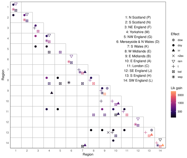
Figure 3: Model selection results. The diagonal corresponds to the elements of $\mathbb{D}_{i}$, the rest to those of $\mathbb{T}_{i}$. The symbols represent different effects and their colour is determined by the magnitude of the element of $\boldsymbol{\Delta}$ corresponding to each effect. Note that the elements of $\mathbb{T}_{i}$ corresponding to the empty cells are not zero, but modelled only via intercepts.

The time of day is used to model also several elements of $\mathbb{T}_{i}$. The strongest such effect, in terms of cumulative log-likelihood gain, acts on the element corresponding to London and the West Midlands (R. 11 and 8). The ALE of $\text{tod}_{i}$ on the correlation between these regions is shown in green in Figure 4e. It shows that prediction errors in these urbanised regions are more correlated during the morning and evening ramps than in the middle of the day. The red curve shows that the correlation between London and the South of England (R. 13) has a similar pattern, although with milder daily oscillations.

Figure 4: Top row: ALEs of the time of day (a), day of year (b), forecasted wind speed (c) and solar irradiation (d) on the standard deviation of net-demand in a selected group of regions. Bottom row: ALEs of same covariates on a selected group of pairwise correlations.

The effect of the day of the year, $\text{doy}_{i}$, is used to model many elements of $\mathbb{D}_{i}$ and $\mathbb{T}_{i}$. It is not surprising to see this effect appearing on the 8th and 11th row of Figure 3, which correspond to the highly urbanised West Midlands (R. 8) and London (R. 11). As the green ALE in Figure 4b shows, net-demand forecast uncertainty is very high in London at the end of the year, due to holidays that have a sizeable, hard-to-model effect on demand patterns. Furthermore, as the effects in Figure 4f show, uncertainty between regions is also highly correlated during this period, meaning that forecast errors are likely to have the same sign across regions as they are driven by the same underlying behavioural effects.

In accordance with intuition, wind speed, $\text{wsp}_{ij}^{100}$, is selected to model the elements of $\mathbb{D}_{i}$ corresponding to regions with a high penetration of embedded wind generation, such as the South East of England (R. 12), and the North (R. 1) and South (R. 2) of Scotland. The ALEs of $\text{wsp}_{ij}^{100}$ in these regions are shown in Figure 4c and could be interpreted as follows. At low wind, the variability of wind production is low because little or no generation is occurring, but it increases at modest wind speeds that are sufficient for power generation to occur, while being in a range where generation is highly sensitive to wind speed. Then variability decreases for high wind speeds, where power production is less variable as turbines self-regulate to maintain their maximum power production. At very high wind speeds, wind turbines may automatically shut down, and small differences in wind speed may result in large differences in production, leading to greater forecast uncertainty.

It is perhaps surprising that wind speed is not selected to control the element of $\mathbb{T}_{i}$ controlling the dependency between the two Scottish GSPs, which both contain large amounts of embedded wind. However, capacity as a fraction of peak load is considerably higher in North than in South of Scotland. Further, the fact that $(\mathbb{T}_{i})_{21}$ is constant, does not mean that the correlation between the two Scottish regions is constant, as illustrated by the green curve in Figure 4g. The plot shows that the correlation is proportional to the variance in these regions, hence wind speed controls both the size and correlation between prediction errors. Interestingly, the blue curve in Figure 4g shows that the net-demand in the South East of England is less correlated with that in London (R. 11) as wind speed in the former region increases, which suggests that this covariate effects the net-demand patterns of these two regions quite differently.

The time of day and solar irradiance, $\text{irr}_{ij}$, are both strongly related to solar energy production, hence it is interesting to see that the effects of both variables are selected to model the elements of $\mathbb{D}_{i}$ corresponding to several Southern regions, which have high embedded solar generation capacity. The ALEs of $\text{irr}_{ij}$ on the net-demand variability in South Wales (R. 7), South (R. 13) and South-West (R. 14) England are shown in Figure 4d. Note that the horizontal scales are different because the installed solar capacity differs between regions. The shape of these effects is similar and could be interpreted as follows. Variability is low at low or high levels of irradiance which correspond to, respectively, heavily clouded (or night) and to clear sky conditions. Variability is highest at intermediate levels of irradiance, which might correspond to partial or broken cloud conditions. However, the shape of the effects may also be affected by the correlation between irradiance and temperature and by changes in installed solar capacity over the study period, hence is it important not to over-interpret them. Solar irradiance is selected to control the dependency between the South of Wales and the South-West of England via the corresponding element of $\mathbb{T}_{i}$. This is interesting because, while the two regions are separated by the Bristol channel, they are geographically close, hence likely to be affected by similar weather patterns, and they both feature very high solar penetration relative to peak load.

As explained above, the set of effects selected by the semi-automated procedure proposed in Section 3.2 matches intuition in many respects. However, looking at Figure 3, note that more than half of the selected effects are related to calendars variables, namely progressive time, time of day, day of year and day of the week. Further, external temperature has not been selected to model any element of $\mathbb{T}_{i}$ or $\mathbb{D}_{i}$. Hence, it is interesting to analyse how the predictive performance of the model depends on the set of candidate covariates that are considered by the model selection procedure. In Section 3.4 we analyse this issue and we compare the proposed model with two non-Gaussian alternatives.

3.4 Model Validation

Here we assess the predictive performance of several alternative models obtained via the selection procedure proposed in Section 3.2. In particular, we consider three sets of candidate effects. The first set (Full) includes all the effects appearing in (3.2), hence it corresponds to the model analysed in Section 3.3. Then we consider a calendar-only model (Cal), obtained by using only the first five effects in (3.2), that is from $g_{j1}(t_{i})$ to $f_{j2}^{10}(\text{tod}_{i})$, and a larger model (Cal+Ren) which also includes the effects of wind speed and solar irradiance. For each set of candidate effects we use data from 2014 to 2017 to perform model selection, as described in Section 3.2 and 3.3. Most of the selected effects in Figure 3 appear on the diagonal, hence we consider also a Cal+Ren Diag model, which is based on the same candidate effects as Cal+Ren, but where Algorithm 1 is allowed to model only the diagonal elements of ${\mathbb{D}}$, while $\mathbb{T}$ is kept constant. This is achieved simply by setting $j=d+1,\dots,2d$ in Step 2.

Having selected the model structure, we assess performance on 2018 data. This is done by first fitting each model to data up to the end of 2017 and then forecasting net-demand during January 2018. We then refit the models to data up to the 31st of January 2018 and forecast net-demand for February. By iterating this rolling forecasting origin procedure, we obtain day-ahead predictions covering the whole of 2018, for each model. To speed up computation, we first fit model (3.2) to the net-demand from each region using separate univariate Gaussian GAMs and then fit the corresponding residuals vectors using each of the covariance matrix models described above, via the methods described in Section 2.2.

We also include in the comparison three models where the marginal distribution of each GSP region’s net-demand is modelled with an increasing amount of flexibility. Two of these models are useful to check whether relaxing the Gaussian assumption improves predictions. In the gaulss+cop model, the net-demand of each region is modelled separately via a univariate location-scale Gaussian model. In shash+cop the net-demand of each region is modelled via the four-parameter sinh-arcsinh distribution of jones2009sinh, which nests the Gaussian but allows for asymmetry and fat-tails. The shash+gpd+cop model produces the same predictions of shash+cop between quantiles 0.05 and 0.95, but uses a generalised Pareto distribution (GPD) beyond these. Having fitted the univariate models separately to each GSP group, we evaluate the corresponding conditional c.d.f.s to obtain uniform residuals. Then we use a static Gaussian copula to model the correlation structure of the resulting 14-dimensional residual vectors. See SM B.2 for more details.

14 GSP groups	Log	Log Ind	CRPS	Pin 001	Pin 999	Var 0.5	Var 1.0
Cal	-3669	-326.8	2582	21.67	44.51	9515	10293
Cal+Ren	-4082	-744.2	2571	20.24	33.97	9298	10012
Full	-4071	-771.9	2570	19.25	34.07	9263	9965
Cal+Ren Diag	-3843	-606.2	2574	20.97	35.45	9299	10014
gaulss+cop	-3786	-646.0	2576	21.05	32.07	9387	10125
shash+cop	-3920	-790.7	2574	20.66	30.31	9355	10097
shash+gpd+cop	-3975	-821.6	2575	20.41	30.59	9362	10116
5 GSP macro-regions	Log	Log Ind	CRPS	Pin 001	Pin 999	Var 0.5	Var 1.0
Cal	3236	4529.7	2008	14.84	42.77	2215	4871
Cal+Ren	3091	4351.1	2000	13.63	34.73	2181	4782
Full	3056	4337.9	1999	12.92	34.58	2170	4756
Cal+Ren Diag	3226	4469.3	2004	14.22	37.77	2188	4802
gaulss+cop	3184	4384.8	2003	14.64	36.59	2183	4788
shash+cop			2002	14.26	35.40	2181	4785
shash+gpd+cop			2003	13.94	37.47	2183	4792

Table 2: Day-ahead performance scores on 2018 test data, when forecasting the joint distribution of net-demand across the 14 GSP groups (top seven rows) or across the five GSP macro-regions (bottom seven rows). The best score in each column has been underlined.

The location parameters of the Gaussian, sinh-arcsinh and GPD models are kept constant because, as for the multivariate Gaussian models, they are fitted to the raw residuals of Gaussian GAMs based on formula (3.2). The effects used to model the scale parameters of the gaulss+cop model are chosen from the same pool of candidates used for Cal+Ren, following the approach described in Section 3.2 but with the following modifications to Algorithm 1. We set all the elements of $\mathbb{T}$ to zero which implies that the diagonal elements of $\mathbb{D}$ are directly controlling the marginal variance of each GSP group’s net-demand (see Section 2.1). Then, as for Cal+Ren Diag, we allow Algorithm 1 to model only the elements of $\mathbb{D}$. In this way, the models for the Gaussian scale parameter are selected to optimise the marginal fit to each region’s net-demand. The resulting effects are used to model the scale parameters of the sinh-arcsinh distribution as well, while the parameters controlling the skewness and kurtosis are modelled only via intercepts. This is because our attempts to manually select a model for them led to a worse performance than what is reported below. Each GPD model is fitted to only 5% of the data, hence we model its scale parameter using only a smooth effect of $\text{tod}_{i}$, while the shape parameter is kept constant.

We use the day-ahead multivariate predictions of each model to compute the performance metrics reported in Table 2. We consider the log score (i.e., the negative log-likelihood), the log score under independence (i.e., the sum of the negative marginal log-likelihoods of each GSP group), the marginal continuous ranked probability score (CRPS, see e.g. gneiting2007) and marginal pinball losses for quantiles 0.001 and 0.999 (each summed over the GSP groups), and the $p$-variogram score (scheuerer2015variogram) with $p=0.5$ and $p=1$.

Considering the first seven rows of Table 2, note that the predictive performance of Cal+Ren is superior to that of Cal on all scores, demonstrating the importance of including covariates that are strongly related to embedded renewable generation. The significance of the improvement is demonstrated by Figure 5a. Here, non-parametric bootstrapping with week-long blocks is used to quantify the variability of the differences in log scores between several pairs of models (SM B.3 provides analogous plots for the remaining scores). The boxplots show that the gain obtained by including the effect of wind and solar irradiation is significant. Instead, extending the set of candidate effects as done in Full does not lead to any gain under the log score, which motivates our choice of basing the copula models on the same pool of candidate effects used for Cal+Ren.

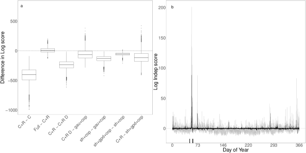
Figure 5: a: Bootstrapped differences in the total log score between several pairs of models. Negative values mean that the first method is better than the second (e.g., Cal+Ren does better than Cal). b: Half-hourly marginal log losses of Cal+Ren (grey) along the test set (2018) and differences between the loss of Cal+Ren and that of shash+gpd+cop model (black). The black ticks mark the start and the end of the Beast from the East cold wave.

Table 2 and Figure 5a show that modelling only the elements of $\mathbb{D}$ as done by Cal+Ren Diag leads to a worse performance, which highlights the importance of modelling $\mathbb{T}$ as well. Interestingly, gaulss+cop does worse than Cal+Ren Diag under the total log score, but better on the independent log score. As both models are Gaussian, this suggests that modelling the marginal variances directly and assuming that the correlation structure is constant, as done by gaulss+cop, leads to better marginal predictions but to a worse multivariate fit, relative modelling the $\mathbb{D}$ factor of the MCD parametrisation, as done by Cal+Ren Diag (recall that $\mathbb{D}$ affects the marginal variances as well as the correlation structure). Similarly, the shash+cop and shash+gpd+cop models have better marginal log scores than Cal+Ren (which uses the same pool of covariates), but worse total log and variogram scores. The fact that the CRPS loss, which is insensitive to tail behaviour (taillardat2023evaluating), is better under the Cal+Ren model suggests that this model is better at predicting intermediate marginal net-demand quantiles while, as demonstrated also by the pinball scores, the non-Gaussian marginal models do better in the upper tail.

To verify this, Figure 5b shows the independent log score of the Cal+Ren model (grey line) and the differences between the Cal+Ren and shash+gpd+cop under the same score (black line). The largest gain of shash+gpd+cop relative to Cal+Ren occurs during the Beast from the East cold wave, which is delimited by the black ticks at the bottom of Figure 5b. All the models considered here struggle to forecast the effect of this weather extreme on net-demand, as the training data does not contain any cold wave of similar magnitude. The better performance of shash+gpd+cop under the independent log score is explained by the fact that this model has fatter tails (recall that the tails are modelled separately from the bulk of the net-demand distribution under this model). To check to what degree the results discussed here are affected by the Beast from the East, in SM B.3 we report a version of Table 2 obtained by excluding this exceptional period from the data. All the results discussed here are still valid but, as expected, excluding the cold wave reduces the benefit of adopting non-Gaussian marginal models.

This work is motivated by the need for spatially coherent probabilistic net-demand forecasts in power flow studies and, as explained in Section 1, the transmission grid boundaries of interest in such studies vary depending on, for example, the status of the network. Hence, it is interesting to verify whether the results discussed above still hold when the forecast is post-processed to match the needs of an operationally relevant scenario. While considering realistic scenarios would require covering engineering aspects that are well beyond the scope of this work, in Section 1 we proposed aggregating the GSP regions into the five macro-regions shown in Figure 1, which were motivated by some of the boundaries of interest described in the 2021 National Grid’s Ten Year Statement (elect10year).

Joint macro-regional net-demand forecasts are easy to obtain, because they are linear transformations of the regional forecasts. The last seven rows of Table 2 show the performance of each model when forecasting the joint distribution of macro-regional net-demand. Note that the scores are on a different scale due to the aggregation of net-demand (5 macro-regions vs 14 regions) and that the log scores have not been computed under two of the model, because the p.d.f. of linear combinations of correlated sinh-arsinh-distributed random variables is, to our best knowledge, not analytically available. The results are similar to those obtained at regional level, but here the Full model produces the best forecasts under all the scores. Due to the high cost of operating power systems (and volume of energy traded in wholesale markets), even marginal improvement in forecast performance and associated decision-making can yield substantial economic and operational benefits.

It is also possible to linearly transform the joint regional forecasts to obtain marginal probabilistic forecasts of differences in net-demand between regions or macro-regions. Such forecasts could be of particular interest in the context of power flow analyses focused on specific transmission grid boundaries. In SM B.3 we assess the performance of the models under three operationally motivated scenarios.

4 Conclusion

Forecasts of supply and demand are essential inputs to predict and manage power flows on electricity networks, as well as prices and other important variables. Given the imperative to maintain a reliable electricity supply, these predictions must enable risk to be quantified and managed. As the complexity of energy systems increases, the heuristic approaches widely used today are becoming inadequate and will have to be replaced by explicit probabilistic forecasts of power flows (morales2013).

Motivated by the need for spatially coherent, probabilistic net-demand forecasts to support energy system operations, we have focused on joint day-ahead forecasting of net-demand across the GSP regions comprising GB’s transmission system. To accommodate for the dynamic nature of the net-demand covariance matrix, we let the elements of its MCD parametrisation vary with a number of temporal and weather-related covariates. To perform effect selection for a model comprising more than one hundred linear predictors, we leverage the interpretability of the chosen parametrisation and we combine it with a semi-automatic effect selection method, based on gradient-boosting. The results on the test set show that additive covariance matrix models significantly outperform, in terms of the total log, CRPS and variogram scores, two non-Gaussian models where the correlation matrix is static. However, the non-Gaussian models provide better predictions of extremely high quantiles, which suggests that a promising direction for future research might be adapting dynamic covariance matrix models to a non-Gaussian context.

A further direction for future work would be to extend the model presented here to capture temporal, in addition to spatial, dependencies. In particular, the covariance matrix models used here implicitly assume that regional net-demand residual vectors are uncorrelated in time. While the mean vector model (3.2) contains the effect of lagged net-demand, which is meant to capture part of the intra-regional temporal dependencies, more complex temporal effects could be captured by extending the covariance matrix to explicitly model the longitudinal nature of the data considered here. Such an extension should lead to models able to generate multivariate net-demand trajectories that are coherent both in space and in time, thus supporting important operations (e.g. determining the schedules for power generating units) that must consider both spatial and temporal constraints.

Supplementary Material to “Additive Covariance Matrix Models: Modelling Regional Electricity Net-Demand in Great Britain”

Note: The numbering of the tables and figures shown below follows from the main text. For example, when we mention Figure 1 below, we refer to Figure 1 in the main text. The first figure in the supplementary material below is Figure 6 because the main text contains 5 figures.

Appendix A Derivatives of the Log-Likelihood

A.1 Setting up the Notation

Consider a scalar-valued function $f$ of the $n$-dimensional vectors ${\boldsymbol{\eta}}_{1},\dots,{\boldsymbol{\eta}}_{q}$. We indicate with $f^{{\boldsymbol{\eta}}_{k}}$ and $f^{{\boldsymbol{\eta}}_{k}{\boldsymbol{\eta}}_{j}}$ the vectors with $i$-th elements

$$f^{\eta_{ik}}=\frac{\partial f}{\partial\eta_{ik}}\quad\text{and}\quad f^{\eta_{ik}\eta_{ij}}=\frac{\partial^{2}f}{\partial\eta_{ik}\partial\eta_{ij}}\,\,,$$

where $\eta_{ik}$ indicates the $i$-th element of ${\boldsymbol{\eta}}_{k}$. Each ${\boldsymbol{\eta}}_{k}$ is a function of a corresponding $p_{k}$-dimensional vector ${\boldsymbol{\beta}}_{k}$. For the derivatives of $f$ w.r.t. the elements of ${\boldsymbol{\beta}}_{k}$, we use the compact notation

$$f^{\beta_{kr}}=\frac{\partial f}{\partial\beta_{kr}}\quad\text{and}\quad f^{\beta_{kr}\beta_{js}}=\frac{\partial^{2}f}{\partial\beta_{kr}\partial\beta_{js}}\,\,,$$

where $\beta_{kr}$ indicates the $r$-th element of ${\boldsymbol{\beta}}_{k}$. Finally, we denote with $f^{{\boldsymbol{\beta}}_{k}}=\nabla_{{\boldsymbol{\beta}}_{k}}f$ the gradient of $f$ w.r.t. ${\boldsymbol{\beta}}_{k}$ and with $f^{{\boldsymbol{\beta}}_{k}{\boldsymbol{\beta}}_{j}}=\nabla_{{\boldsymbol{\beta}}_{j}}^{\top}\nabla_{{\boldsymbol{\beta}}_{k}}f$ the matrix of second derivatives.

A.2 Gradient and Hessian w.r.t. ${\boldsymbol{\beta}}$

To simplify the notation, let us indicate with $\mathbb{y}$ the collection of all response vectors $\mathbb{y}_{1},\dots,\mathbb{y}_{n}$ and define $\mathcal{L}({\boldsymbol{\beta}})=\log p({\boldsymbol{\beta}}|\mathbb{y},{\boldsymbol{\lambda}})$. Recall that

$$\mathcal{L}({\boldsymbol{\beta}})=\sum_{i=1}^{n}\ell_{i}-\frac{1}{2}{\boldsymbol{\beta}}^{\top}\tilde{\bf S}^{\boldsymbol{\lambda}}{\boldsymbol{\beta}}$$

where $\ell_{i}=\log p(\mathbb{y}_{i}|{\boldsymbol{\beta}})$. The gradient and Hessian of the log-posterior w.r.t ${\boldsymbol{\beta}}$ are

$$\mathcal{L}^{{\boldsymbol{\beta}}}({\boldsymbol{\beta}})=\sum_{i=1}^{n}\ell_{i}^{{\boldsymbol{\beta}}}-\tilde{\mathbf{S}}^{{\boldsymbol{\lambda}}}{\boldsymbol{\beta}}\quad\text{and}\quad\mathcal{L}^{{\boldsymbol{\beta}}{\boldsymbol{\beta}}}({\boldsymbol{\beta}})=\sum_{i=1}^{n}\ell_{i}^{{\boldsymbol{\beta}}{\boldsymbol{\beta}}}-\tilde{\mathbf{S}}^{{\boldsymbol{\lambda}}}\,\,.$$

Let us define $\bar{\ell}=\sum_{i=1}^{n}\ell_{i}$ . To provide formulas for $\bar{\ell}^{{\boldsymbol{\beta}}}$ and $\bar{\ell}^{{\boldsymbol{\beta}}{\boldsymbol{\beta}}}$, let us assume that ${\boldsymbol{\beta}}=({{\boldsymbol{\beta}}_{1}}^{\top},\dots,{{\boldsymbol{\beta}}_{q}}^{\top})^{\top}$, where ${\boldsymbol{\beta}}_{j}$ is the vector of regression coefficients specific to the $j$-th linear predictor, that is ${\boldsymbol{\eta}}_{j}=\mathbf{X}^{j}{\boldsymbol{\beta}}_{j}$ where $\mathbf{X}^{j}$ is an $n\times p_{j}$ model matrix. With this notation, the $j$-th sub-vector of $\bar{\ell}^{{\boldsymbol{\beta}}}$ is

$$\bar{\ell}^{{\boldsymbol{\beta}}_{j}}={\mathbf{X}^{j}}^{\top}\ell^{{\boldsymbol{\eta}}_{j}}\,\,,$$

while the $j,k$-th block of the Hessian is

$$\bar{\ell}^{{\boldsymbol{\beta}}_{j}{\boldsymbol{\beta}}_{k}}=(\bar{\ell}^{{\boldsymbol{\beta}}_{k}{\boldsymbol{\beta}}_{j}})^{\top}={\mathbf{X}^{k}}^{\top}\text{diag}(\ell^{{\boldsymbol{\eta}}_{j}{\boldsymbol{\eta}}_{k}}){\mathbf{X}^{j}}\,\,,$$

where ${\rm diag}(\cdot)$ is the vector-to-matrix diagonal operator. The formulas provided so far are applicable to any GAM with multiple linear predictors and independent response vectors. In contrast, the expressions for $\ell^{{\boldsymbol{\eta}}_{j}}$ and $\ell^{{\boldsymbol{\eta}}_{j}{\boldsymbol{\eta}}_{k}}$ are model-specific and are provided in the following section for a multivariate Gaussian distribution, with covariance matrix parametrised via the MCD.

A.3 Derivatives w.r.t. ${\boldsymbol{\eta}}$

Let us start by defining a few useful quantities. Let $\mathbb{G}$ be a $(d-1)\times(d-1)$ lower triangular matrix such that $G_{jk}=C_{jk}+2d\mathbbm{1}_{\{k\leq j\}}$, where

$${\rm C}_{jk}=\begin{cases}\quad\binom{j+1}{2}\quad\quad\quad\,\,\,k=j\\ {\rm C}_{j(k+1)}-1\quad\quad\,k<j\\ \quad\quad 0\quad\quad\quad\quad\,\,k>j\,\,,\end{cases}$$

and $\mathbbm{1}$ is the indicator function. Define the $(d-1)\times(d-1)$ lower triangular matrices $\mathbb{Z}$ and $\mathbb{W}$ such that ${\rm Z}_{jk}=k\mathbbm{1}_{\{k\leq j\}}$ and ${\rm W}_{jk}=(j+1)\mathbbm{1}_{\{k\leq j\}}$. Let $\mathbb{z}=\operatorname{rvech}(\mathbb{Z})$ and $\mathbb{w}=\operatorname{rvech}(\mathbb{W})$, where $\operatorname{rvech}(\cdot)$ is the row-wise half-vectorisation operator, that is $\operatorname{rvech}(\mathbb{Z})=(Z_{11},Z_{21},Z_{22},Z_{31},Z_{32},Z_{33},\dots,Z_{(d-1)(d-1)})^{\top}$. Let $\mathbb{Q}_{l}$, for $l=1,\ldots,d$, and $\mathbb{P}_{l}$, for $l=1,\ldots,d(d-1)/2$, be $d\times d$ matrices such that $(\mathbb{Q}_{l})_{ll}=e^{-\eta_{l+d}}$ and $(\mathbb{P}_{l})_{{z}_{l}{w}_{l}}=1$, while all other elements are equal to zero.

Here index $i$ is not needed, hence we drop it and we indicate the $i$-th log-likelihood component $\ell_{i}$ simply with $\ell$. Note that, given that we are focusing on an individual $i$, here ${\boldsymbol{\eta}}$ is a $q$-dimensional vector and $q=d+d(d+1)/2$. If we omit the constants that do not depend on ${\boldsymbol{\eta}}$ and we indicate with $r_{k}$ the $k$-th element of the residual vector, $\mathbb{r}=\mathbb{y}-\boldsymbol{\mu}$, the Gaussian log-density can be written

$$\ell =-\frac{1}{2}\left\{{\rm tr}(\log\mathbb{D}^{2})+\mathbb{r}^{\top}\mathbb{T}^{\top}\mathbb{D}^{-2}\mathbb{T}\mathbb{r}\right\}$$

$$=-\frac{1}{2}\sum_{j=1}^{d}\Big{\{}\eta_{j+d}+e^{-\eta_{j+d}}\Big{(}\sum_{k=1}^{j-1}\eta_{{\rm G}_{(j-1)k}}r_{k}+r_{j}\Big{)}^{2}\Big{\}}\,\,,$$

where we used $\log|\boldsymbol{\Sigma}|={\rm tr}(\log\mathbb{D}^{2})=\sum_{j=1}^{d}\eta_{j+d}$ and we implicitly assumed that the sum $\sum_{k=1}^{j-1}$ should not be computed when $j=1$ (we will use the same convention in several places below). Similarly, below we assume that $\sum_{j=l+1}^{d}$ will not be computed when $l=d$. Here we provide the first and second derivatives of $\ell$ w.r.t. ${{\boldsymbol{\eta}}}$ both in compact matrix form and in an extended format, the latter being more useful for efficient numerical implementation.

With notation above, the elements of $\ell^{{\boldsymbol{\eta}}}=(\ell_{1}^{{\boldsymbol{\eta}}},\dots,\ell_{q}^{{\boldsymbol{\eta}}})^{\top}=(\partial\ell/\partial\eta_{1},\dots,\partial\ell/\partial\eta_{q})^{\top}$ are

$$\ell^{{\boldsymbol{\eta}}}_{l} =\left(\mathbb{T}^{\top}\mathbb{D}^{-2}\mathbb{T}\mathbb{r}\right)_{l}$$

$$=e^{-\eta_{d+l}}\Big{(}\sum_{k=1}^{l-1}\eta_{{\rm G}_{(l-1)k}}r_{k}+r_{l}\Big{)}+\sum_{j=l+1}^{d}e^{-\eta_{j+d}}\Big{(}\sum_{k=1}^{j-1}\eta_{{\rm G}_{(j-1)k}}r_{k}+r_{j}\Big{)}\eta_{{\rm G}_{(j-1)l}}\,\,,$$

for $l=1,\ldots,d$,

$$\ell^{{\boldsymbol{\eta}}}_{l} =\frac{1}{2}\mathbb{r}^{\top}\mathbb{T}^{\top}\mathbb{Q}_{l-d}\mathbb{T}\mathbb{r}-\frac{1}{2}$$

$$=\frac{1}{2}e^{-\eta_{l}}\Big{(}\sum_{k=1}^{l-d-1}\eta_{{\rm G}_{(l-d-1)k}}r_{k}+r_{l-d}\Big{)}^{2}-\frac{1}{2}\,\,,$$

for $l=d+1,\ldots,2d$, and

$$\ell^{{\boldsymbol{\eta}}}_{l} =-\mathbb{r}^{\top}\mathbb{P}_{l-2d}\mathbb{D}^{-2}\mathbb{T}\mathbb{r}$$

$$=-e^{\eta_{w_{l-2d}+d}}\Big{(}\sum_{k=1}^{w_{l-2d}-1}\eta_{{\rm G}_{(w_{l-2d}-1)k}}r_{k}+r_{w_{l-2d}}\Big{)}r_{z_{l-2d}}\,\,,$$

for $l=2d+1,\ldots,q$.

The elements forming the upper triangle of $\ell^{{\boldsymbol{\eta}}{\boldsymbol{\eta}}}$ (here $\ell^{{\boldsymbol{\eta}}{\boldsymbol{\eta}}}_{lm}=\partial^{2}\ell/\partial\eta_{l}\partial\eta_{m}$), are

$$\ell^{{\boldsymbol{\eta}}{\boldsymbol{\eta}}}_{lm} =-\left(\mathbb{T}^{\top}\mathbb{D}^{-2}\mathbb{T}\right)_{lm}$$

$$=-\Big{\{}e^{-{\eta}_{l+d}}+\sum_{k=l+1}^{d}e^{-{\eta}_{k+d}}\Big{(}{\eta}_{{\rm G}_{(k-1)l}}\Big{)}^{2}\Big{\}}\mathbbm{1}_{\{m=l\}}$$

$$\hskip 14.22636pt-\Big{(}e^{-{\eta}_{m+d}}{\eta}_{{\rm G}_{(m-1)l}}+\sum_{k=m+1}^{d}e^{-{\eta}_{k+d}}{\eta}_{{\rm G}_{(k-1)l}}{\eta}_{{\rm G}_{(k-1)m}}\Big{)}\mathbbm{1}_{\{m>l\}}\,\,,$$

for $l=1,\ldots,d,$ and $m=l,\ldots,d$,

$$\ell^{{\boldsymbol{\eta}}{\boldsymbol{\eta}}}_{lm} =-\left(\mathbb{T}^{\top}\mathbb{Q}_{m-d}\mathbb{T}\mathbb{r}\right)_{l}$$

$$=-e^{-{\eta}_{m}}\Big{\{}\Big{(}\sum_{k=1}^{l-1}\eta_{G_{(l-1)k}}r_{k}+r_{l}\Big{)}\mathbbm{1}_{\{m-d=l\}}$$

$$\hskip 14.22636pt+\Big{(}\sum_{k=1}^{m-d-1}\eta_{G_{(m-d-1)k}}r_{k}+r_{m-d}\Big{)}\eta_{G_{(m-d-1)l}}\mathbbm{1}_{\{m-d>l\}}\Big{\}}\,\,,$$

for $l=1,\ldots,d,$ and $m=d+1,\ldots,2d$,

$$\ell^{{\boldsymbol{\eta}}{\boldsymbol{\eta}}}_{lm} =\left(\mathbb{P}_{m-2d}\mathbb{D}^{-2}\mathbb{T}\mathbb{r}+\mathbb{T}^{\top}\mathbb{D}^{-2}\mathbb{P}^{\top}_{m-2d}\mathbb{r}\right)_{l}\,\,$$

$$=e^{-\eta_{w_{m-2d}+d}}\Big{\{}r_{z_{m-2d}}\Big{(}\mathbbm{1}_{\{w_{m-2d}=l\}}+\eta_{{\rm G}_{(w_{m-2d}-1)l}}\mathbbm{1}_{\{w_{m-2d}>l\}}\Big{)}$$

$$\hskip 14.22636pt+\Big{(}\sum_{k=1}^{w_{m-2d}-1}\eta_{{\rm G}_{(w_{m-2d}-1)k}}r_{k}+r_{w_{m-2d}}\Big{)}\mathbbm{1}_{\{z_{m-2d}=l\}}\Big{\}}\,\,,$$

for $l=1,\ldots,d,$ and $m=2d+1,\ldots,q$,

$$\ell^{{\boldsymbol{\eta}}{\boldsymbol{\eta}}}_{lm} =-\frac{1}{2}\mathbb{r}^{\top}\mathbb{T}^{\top}\mathbb{Q}_{l-d}\mathbb{T}\mathbb{r}$$

$$=-\frac{1}{2}e^{-\eta_{l}}\Big{(}\sum_{k=1}^{l-d-1}\eta_{{\rm G}_{(l-d-1)k}}r_{k}+r_{l-d}\Big{)}^{2}\mathbbm{1}_{\{m=l\}}\,\,,$$

for $l=d+1,\ldots,2d,$ and $m=l,\ldots,2d$,

$$\ell^{{\boldsymbol{\eta}}{\boldsymbol{\eta}}}_{lm} =\mathbb{r}^{\top}\mathbb{P}_{m-2d}\mathbb{Q}_{l-d}\mathbb{T}\mathbb{r}$$

$$=e^{-\eta_{l}}\Big{(}\sum_{k=1}^{l-d-1}\eta_{{\rm G}_{(l-d-1)k}}r_{k}+r_{l-d}\Big{)}r_{z_{m-2d}}\mathbbm{1}_{\{w_{m-2d}=l-d\}}\,\,,$$

for $l=d+1,\ldots,2d,$ and $m=2d+1,\ldots,q$, and finally

$$\ell^{{\boldsymbol{\eta}}{\boldsymbol{\eta}}}_{lm} =-\mathbb{r}^{\top}\mathbb{P}_{l-2d}\mathbb{D}^{-2}\mathbb{P}^{\top}_{m-2d}\mathbb{r}$$

$$=-e^{-{\eta}_{w_{l-2d}+d}}r_{z_{l-2d}}r_{z_{m-2d}}\mathbbm{1}_{\{w_{m-2d}=w_{l-2d}\}}\,\,,$$

for $l=2d+1,\ldots,q,$ and $m=l,\ldots,q$.

A.4 Details on accumulated local effects

Recall that ${\boldsymbol{\Sigma}}_{i}$ depends on the covariate vector $\boldsymbol{x}_{i}$ via the linear predictor vector ${\boldsymbol{\eta}}_{i}$. By omitting the subscript $i$ and expliciting the dependence on $\boldsymbol{x}$, let us denote with $\omega(\boldsymbol{x})$ a generic element of ${\boldsymbol{\Sigma}}$ or of the correlation matrix $\boldsymbol{\Gamma}$, the elements of the latter being defined by $\Gamma_{jk}=\Sigma_{jk}/\sqrt{\Sigma_{jj}\Sigma_{kk}}$. Assuming that $\omega(\boldsymbol{x})$ is differentiable w.r.t. the $k$-th covariate, the main (first-order) accumulated local effects (ALEs) of $x_{k}$ is

$$\mkern 1.5mu\overline{\mkern-1.5mu\omega\mkern-1.5mu}\mkern 1.5mu_{k}(x)=\int_{x_{k}^{\text{min}}}^{x}\mathbb{E}_{{\boldsymbol{x}}_{\backslash k}}\left\{\omega^{k}(z,{\boldsymbol{x}}_{\backslash k})|x_{k}=z\right\}dz-\text{constant}\,\,,$$

where ${\boldsymbol{x}}_{\backslash k}$ is ${\boldsymbol{x}}$ with the $k$-th element excluded, $\omega^{k}=\partial\omega/\partial x_{k}$ and $\mathbb{E}_{{\boldsymbol{x}}_{\backslash k}}\{\cdot|x_{k}=z\}$ is the conditional expectation w.r.t. $p({\boldsymbol{x}}_{\backslash k}|x_{k}=z)$. The choice $x_{k}^{\text{min}}$ is unimportant, as changing it simply shifts the effect vertically, so in practice $x_{k}^{\text{min}}$ is set to just below the smallest observed value of $x_{k}$.

An uncentered first-order ALE is obtained by setting the constant term to zero, while a centered ALE has a mean equal to zero, when averaged over the observed values of the covariate of interest. This is explained by apley2020, who also provide formulas for obtaining estimated effects ${\hat{\mkern 1.5mu\overline{\mkern-1.5mu\omega\mkern-1.5mu}\mkern 1.5mu}}_{k}(x)$, by approximating the integral above. For instance, consider an uncentered ALE and let $x_{ik}$ be the $i$-th observed value of $x_{k}$. Further, denote with $z_{0k},\ldots,z_{Bk}$ a grid of values along $x_{k}$, with $z_{0k}=\min_{i=1,\ldots,n}x_{ik}$ and $z_{Bk}=\max_{i=1,\ldots,n}x_{ik}$, and let $n_{k}(1),\ldots,n_{k}(B)$ the number of $x_{ik}$ included, respectively, in the intervals $N_{k}(1)=[z_{0k},z_{1k}),\ldots,N_{k}(B)=[z_{B-1k},z_{Bk}]$. Then, the ALE of $x_{k}$ is estimated via

$${\hat{\mkern 1.5mu\overline{\mkern-1.5mu\omega\mkern-1.5mu}\mkern 1.5mu}}_{k}(x)=\sum_{v=1}^{v_{k}(x)}\frac{1}{n_{k}(v)}\sum_{\{i:x_{ik}\in N_{k}(v)\}}\{\omega(z_{vk},\boldsymbol{x}_{i\backslash k})-\omega(z_{v-1k},\boldsymbol{x}_{i\backslash k})\}$$

with ${\hat{\mkern 1.5mu\overline{\mkern-1.5mu\omega\mkern-1.5mu}\mkern 1.5mu}}_{k}(z_{0k})=0$ and $v_{k}(x)\in\{1,\ldots,B\}$ denoting the bin number to which an arbitrary value $x$ of $x_{k}$ belongs.

The uncertainty of ALEs can be quantified by propagating posterior parameter uncertainty via a standard asymptotic approximation. Recall that standard Bayesian asymptotics justify approximating $p({\boldsymbol{\beta}}|\mathbb{y},{\boldsymbol{\lambda}})$ with a Gaussian distribution, $N(\hat{{\boldsymbol{\beta}}},{\bf V}_{{\boldsymbol{\beta}}})$, centered at the MAP estimate and with covariance matrix ${\bf V}_{{\boldsymbol{\beta}}}=-\boldsymbol{\mathcal{H}}^{-1}$, where $\boldsymbol{\mathcal{H}}$ is the negative Hessian of $\log p({\boldsymbol{\beta}}|\mathbb{y},{\boldsymbol{\lambda}})$, evaluated at $\hat{\boldsymbol{\beta}}$. capezza2021additive show that, in a GAM context, the delta method can be used to approximate the posterior variance of ALEs via $\text{var}\{{\hat{\mkern 1.5mu\overline{\mkern-1.5mu\omega\mkern-1.5mu}\mkern 1.5mu}}_{k}(x)\}\approx\nabla_{{\boldsymbol{\beta}}}^{\top}{\hat{\mkern 1.5mu\overline{\mkern-1.5mu\omega\mkern-1.5mu}\mkern 1.5mu}}_{k}{\bf V}_{{\boldsymbol{\beta}}}\nabla_{{\boldsymbol{\beta}}}{\hat{\mkern 1.5mu\overline{\mkern-1.5mu\omega\mkern-1.5mu}\mkern 1.5mu}}_{k}$. The authors provide formulas for the Jacobian $\nabla_{{\boldsymbol{\beta}}}{\hat{\mkern 1.5mu\overline{\mkern-1.5mu\omega\mkern-1.5mu}\mkern 1.5mu}}_{k}(x)$ that apply to any GAM with multiple linear predictors, covering also the case where $x_{k}$ is a categorical variable. Below we provide the details for obtaining the Jacobian $\nabla_{{\boldsymbol{\beta}}}{\hat{\mkern 1.5mu\overline{\mkern-1.5mu\omega\mkern-1.5mu}\mkern 1.5mu}}_{k}(x)$, where the only output-specific component is the Jacobian of the parametrisation linking $\omega(\boldsymbol{x})$ with ${\boldsymbol{\eta}}$.

Suppose that the output of interest, $\omega(\boldsymbol{x})$, is an element of ${\boldsymbol{\Sigma}}$. Define the vector $\boldsymbol{\sigma}_{jk}=\{({\boldsymbol{\Sigma}}_{1})_{jk},\dots,({\boldsymbol{\Sigma}}_{n})_{jk}\}^{\top}$ and consider the vector containing the values of the $j$-th linear predictor at each observation, that is ${{\boldsymbol{\eta}}}_{j}=(\eta_{1j},\dots,\eta_{nj})^{\top}$. For $j=1,\dots,q$, we have that ${\boldsymbol{\eta}}_{j}={\mathbb{X}}^{j}{\boldsymbol{\beta}}_{j}$ where ${\mathbb{X}}^{j}$ and ${\boldsymbol{\beta}}_{j}$ are, respectively, the $n\times p_{j}$ model matrix and the $p_{j}$-dimensional vector of regression coefficients belonging to the $j$-th linear predictor. The, the $n\times p$ Jacobian matrix of $\boldsymbol{\sigma}_{jk}$ w.r.t. ${\boldsymbol{\beta}}$ is

$$\mathbf{J}^{jk}=\nabla_{{\boldsymbol{\beta}}}^{\top}\boldsymbol{\sigma}_{jk}=(\nabla_{{\boldsymbol{\beta}}_{1}}^{\top}\boldsymbol{\sigma}_{jk},\cdots,\nabla_{{\boldsymbol{\beta}}_{q}}^{\top}\boldsymbol{\sigma}_{jk})\,\,,$$

where $p=\sum_{j=1}^{q}p_{j}$. The $a$-th block of $\mathbf{J}^{jk}$ is

$$\nabla_{{\boldsymbol{\beta}}_{a}}^{\top}\boldsymbol{\sigma}_{jk}=\nabla_{{\boldsymbol{\eta}}_{a}}^{\top}\boldsymbol{\sigma}_{jk}\nabla^{\top}_{{\boldsymbol{\beta}}_{a}}{{\boldsymbol{\eta}}_{a}}=\nabla_{{\boldsymbol{\eta}}_{a}}^{\top}\boldsymbol{\sigma}_{jk}{\bf X}^{a}\,\,,$$

for $a=1,\dots,q$, and where $\nabla_{{\boldsymbol{\eta}}_{a}}^{\top}\boldsymbol{\sigma}_{jk}$ is an $n\times n$ diagonal matrix with non-zero elements

$$\left(\nabla_{{\boldsymbol{\eta}}_{a}}^{\top}\boldsymbol{\sigma}_{jk}\right)_{ii}=\frac{\partial({\boldsymbol{\Sigma}}_{i})_{jk}}{\partial\eta_{ia}}\,\,.$$

Note $\partial({\boldsymbol{\Sigma}}_{i})_{jk}/\partial\eta_{ia}$ is the only parametrisation-dependent component of the Jacobian, thus in Section A.4.1 we provide the relevant formulas. When $\omega(\boldsymbol{x})$ is an element of $\mathbb{\Gamma}$, the posterior variance of the ALEs is approximated similarly, since the Jacobian of $\{(\boldsymbol{\Gamma}_{1})_{jk},\dots,(\boldsymbol{\Gamma}_{n})_{jk}\}$ w.r.t. ${\boldsymbol{\beta}}$ is computed analogously, but with $\partial(\boldsymbol{\Gamma}_{i})_{jk}/\partial\eta_{ia}$ in place of $\partial({\boldsymbol{\Sigma}}_{i})_{jk}/\partial\eta_{ia}$. Formulas for $\partial(\boldsymbol{\Gamma}_{i})_{jk}/\partial\eta_{ia}$ are provided in Section A.4.2.

A.4.1 Derivatives of $\boldsymbol{\Sigma}$ w.r.t. ${\boldsymbol{\eta}}$

Here the index $i$ is not needed, hence we drop it. Consider the factorisation $\boldsymbol{\Sigma}=\mathbb{R}\mathbb{R}^{\top}$ where $\mathbb{R}=\mathbb{L}\mathbb{D}$ and $\mathbb{L}=\mathbb{T}^{-1}$. The partial derivative of the $(l,m)$ element of $\boldsymbol{\Sigma}$ w.r.t. $\eta_{j}$, is

$$\frac{\partial\Sigma_{lm}}{\partial\eta_{j}}=\sum_{k=1}^{d}\left(\frac{\partial{\rm R}_{lk}}{\partial\eta_{j}}{\rm R}_{mk}+{\rm R}_{lk}\frac{\partial{\rm R}_{mk}}{\partial\eta_{j}}\right),$$

where

$$\frac{\partial{\rm R}_{lk}}{\partial\eta_{j}}=0\,\,,\quad\text{for}\quad j=1,\ldots,d,$$

$$\frac{\partial{\rm R}_{lk}}{\partial\eta_{j}}=\frac{\partial{\rm L_{lk}}{\rm D_{kk}}}{\partial\eta_{j}}=\frac{1}{2}{\rm L_{l(j-d)}}{\rm D_{(j-d)(j-d)}}\mathbbm{1}_{\{j-d=k\}}\,\,,\quad\text{for}\quad j=d+1,\ldots,2d,$$

and

$$\frac{\partial{\rm R}_{lk}}{\partial\eta_{j}}=\frac{\partial{\rm L_{lk}}{\rm D_{kk}}}{\partial\eta_{j}}=-{\rm L_{ls}}{\rm L_{tk}}{\rm D_{kk}}\,\,,\quad\text{for}\quad j=2d+1,\ldots,q,$$

with $t$ and $s$ being the row and column indices of the only element of $\mathbb{T}$ that depends on $\eta_{j}$, for $j=2d+1,\ldots,q$. Hence, we obtain

$$\frac{\partial\Sigma_{lm}}{\partial\eta_{j}}=0\,\,,\quad\text{for}\quad j=1,\ldots,d,$$

$$\frac{\partial\Sigma_{lm}}{\partial\eta_{j}}={\rm L_{l(j-d)}}{\rm L_{m(j-d)}}{\rm D_{(j-d)(j-d)}}\,\,,\quad\text{for}\quad j=d+1,\ldots,2d,$$

and

$$\frac{\partial\Sigma_{lm}}{\partial\eta_{j}}=-{\rm L_{ls}}\sum_{k=1}^{d}{\rm L_{tk}}{\rm D^{2}_{kk}}{\rm L_{mk}}-{\rm L_{ms}}\sum_{k=1}^{d}{\rm L_{lk}}{\rm D^{2}_{kk}}{\rm L_{tk}}\,\,,\quad\text{for}\quad j=2d+1,\ldots,q,$$

where $t$ and $s$ are defined as above.

A.4.2 Derivatives of $\boldsymbol{\Gamma}$ w.r.t. ${\boldsymbol{\eta}}$

To simplify the notation indicate $(\Sigma_{ll})^{-1/2}$ with $\Sigma^{-1/2}_{ll}$. The $(l,m)$ element of $\boldsymbol{\Gamma}$ is

$$\Gamma_{lm}=\Sigma^{-1/2}_{ll}\,\Sigma_{lm}\,\Sigma^{-1/2}_{mm}\,\,,$$

and its partial derivative w.r.t. $\eta_{j}$, for $j=1,\dots,q$, is

$$\frac{\partial\Gamma_{lm}}{\partial\eta_{j}}=\Sigma^{-1/2}_{ll}\,\frac{\partial\Sigma_{lm}}{\partial\eta_{j}}\,\Sigma^{-1/2}_{mm}-\frac{1}{2}\Sigma_{lm}\Bigg{\{}\Sigma^{-3/2}_{ll}\,\Sigma^{-1/2}_{mm}\,\frac{\partial\Sigma_{ll}}{\partial\eta_{j}}+\Sigma^{-1/2}_{ll}\,\Sigma^{-3/2}_{mm}\,\frac{\partial\Sigma_{mm}}{\partial\eta_{j}}\Bigg{\}}\,\,,$$

and where the derivatives of the elements of ${\boldsymbol{\Sigma}}$ w.r.t. $\eta_{j}$ are provided in Section A.4.1.

Appendix B Further details and results

B.1 Integrating penalised least squares in Algorithm 1

Following the notation from Algorithm 1, let ${\mathbb{u}}_{j}$ be the $j$-th gradient vector and let ${\mathbb{X}}^{r}$ be the model matrix of the $r$-th base learner. To include a generalised ridge penalty in Algorithm 1 it is sufficient to substitute the projection of ${\mathbb{u}}_{j}$ onto ${\mathbb{X}}^{r}$ with the penalised least squares estimator

$$\hat{\mathbb{u}}_{j}^{r}=\mathbb{X}^{r}({\mathbb{X}^{r}}^{\top}\mathbb{X}^{r}+\zeta_{r}{\bf S}_{r})^{-1}{{\mathbb{X}}^{r}}^{\top}\mathbb{u}_{j},$$

where ${\bf S}_{r}$ is a positive semi-definite penalty matrix and $\zeta_{r}>0$.

To mitigate effect selection bias, the scaling parameter $\zeta_{r}$ of the penalty corresponding to each effect should be chosen so that all the effects have similar effective degrees of freedom (hofner2011framework). The latter are defined as

$$\text{edf}_{r}={\rm tr}{\left\{\mathbb{X}^{r}({\mathbb{X}^{r}}^{\top}\mathbb{X}^{r}+\zeta_{r}{\bf S}_{r})^{-1}{{\mathbb{X}}^{r}}^{\top}\right\}},$$

and depend on $\zeta_{r}$. In particular, assuming that $\mathbb{X}^{r}$ is of full rank $p_{r}$ and that ${\bf S}_{r}$ has rank $s_{r}\leq p_{r}$, as $\zeta_{r}$ increases from zero to infinity the $\text{edf}_{r}$ decrease from $p_{r}$ to $p_{r}-s_{r}$.

For each effect appearing in the MCD model (3.2) such that $p_{r}>4$, we choose $\zeta_{r}$ such that $\text{edf}_{r}=4$. This is a one-dimensional numerical optimisation problem, which can be solved very rapidly prior to running Algorithm 1. The effect of progressive time $t_{i}$ is modelled using two parameters, hence penalisation is unnecessary. The penalty matrices ${\bf S}_{r}$ correspond to cubic splines penalties (i.e., proportional to the integrated second derivative of the effect, $\int f^{\prime\prime}(x)^{2}dx$) for all the smooth effects in Algorithm 1, while a standard ridge penalty is used for the effect of the factor $\text{dow}_{i}$.

B.2 Details on the implementation of the copula-based models

The gaulss+cop, shash+cop and shash+gpd+cop GAMLSS models (rigby2005generalized) from Section 3.4 model the marginal distribution of regional net-demand separately from the correlation structure. Here we give more details on the structure of these models and on how they are fitted to data.

Consider the shash+cop model. Under this model, the net-demand from $j$-th region follows a conditional sinh-arcsinh distribution (jones2009sinh), controlled by the four dimensional parameter vector $\boldsymbol{\theta}_{ij}$. Each element of $\boldsymbol{\theta}_{ij}$ could potentially be modelled additively but, for the reasons put forward in Section 3.4, we let only the log-scale parameter depend on the covariates, and control the location, asymmetry and tail parameters only via intercepts. The gaulss+cop model uses a two-parameter conditional Gaussian model, where the location parameter is kept constant while the log-scale parameter is modelled additively, as explained in Section 3.4.

The predictions of the shash+gpd+cop model are based on the same conditional sinh-arcsinh distribution of shash+cop between quantiles 0.05 and 0.95, and on two separate models based on the generalised Pareto distribution (GPD) beyond them. In particular, let $F_{j}(\cdot|{\boldsymbol{x}}_{i})$ be the conditional c.d.f. of the sinh-arcsinh model corresponding to the $i$-th observation and the $j$-th GSP group. Then $q_{ij}^{95}=F^{-1}_{j}(0.95|{\boldsymbol{x}}_{i})$ is an estimate of the 95th conditional net-demand percentile under this model. A two-parameter (scale and location) conditional GPD GAMLSS model is fitted to the observed net-demand values that fall above $q_{ij}^{95}$ and a separate GPD model is fitted to those falling below $q_{ij}^{5}$. Given that each of these models is fitted to only around 5% of the data, we model only the log-scale parameter using a smooth effect of the time of day, while the shape parameter is controlled only by an intercept. Having fitted the sinh-arcsinh and the two GPD models, we build a composite model where the sinh-arcsinh model is used to produce predictions between quantiles 0.05 and 0.95, while the GPD models are used to produce tail predictions.

We fit the 14 conditional Gaussian, sinh-arcsinh and (pairs of) GPD models separately to the net-demand of each region, using the fitting methods of wood2016 and the rolling forecasting approach described in Section 3.4. In a second step, the correlation of net-demand across the GSP groups is modelled as follows. Let $F_{j}(\cdot|{\boldsymbol{x}}_{i})$ be the conditional c.d.f. of the Gaussian, sinh-arcsinh or of the composition of the sinh-arcsinh and the GPD models corresponding to the $i$-th observation and the $j$-th GSP group. If a marginal net-demand model is well specified, $u_{ij}=F_{j}(y_{ij}|{\boldsymbol{x}}_{i})$ should approximately follow a uniform distribution $U(0,1)$ and $z_{ij}=\Phi^{-1}(u_{ij})$, where $\Phi^{-1}(\cdot)$ is the inverse standard Gaussian c.d.f., should follow a standard Gaussian distribution, $N(0,1)$. We then adopt a Gaussian copula model by assuming that the $z_{ij}$’s follow a joint multivariate Gaussian distribution, that is

$${\boldsymbol{z}}_{i}=\begin{pmatrix}z_{i1}\\ z_{i2}\\ z_{i3}\\ \vdots\\ z_{i14}\end{pmatrix}\sim\text{N}\left(\begin{pmatrix}0\\ 0\\ 0\\ \vdots\\ 0\end{pmatrix},\begin{pmatrix}1&\rho_{1,2}&\rho_{1,3}&\cdots&\rho_{1,14}\\ \rho_{1,2}&1&\rho_{2,3}&\cdots&\rho_{2,14}\\ \rho_{1,3}&\rho_{2,3}&1&\cdots&\rho_{3,14}\\ \vdots&\vdots&\vdots&\ddots&\vdots&\\ \rho_{1,14}&\rho_{2,14}&\cdots&\rho_{13,14}&1\\ \end{pmatrix}\right).$$

The parameters, $\rho_{1,2},\dots,\rho_{13,14}$, of the copula model are estimated simply by computing the empirical correlation matrix of the ${\boldsymbol{z}}_{i}$ vectors on the training data, using the same rolling forecasting origin used for the multivariate Gaussian models based on the MCD parametrisation, which ensures that all the models are fitted exactly to the same training data.

B.3 Additional results on UK regional net-demand forecasting

Figure 6 shows the bootstrapped differences between the performance scores of several pairs of models, under the scores shown in columns two to seven of Table 2. The interpretation of the plots is analogous to that of Figure 5a.

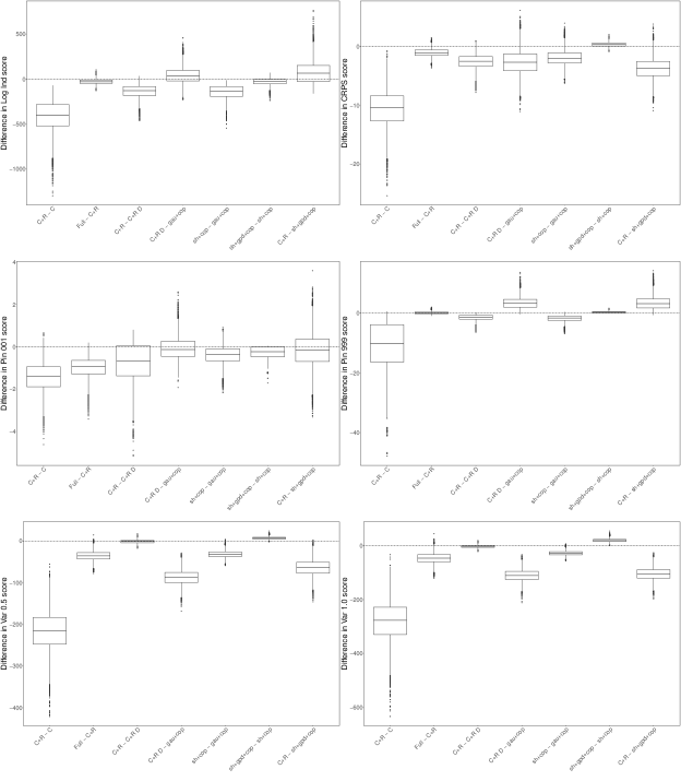
Figure 6: Bootstrapped differences between the scores of several pairs of models, for the performance score shown in columns two to seven of Table 2. Negative values mean that the first method is better than the second (e.g., Cal+Ren does better than Cal under all the scores). Note: The numbering of the figures shown here follows from the main text.

As mentioned in Section 3.4, it is possible to linearly transform the joint regional forecasts to obtain marginal probabilistic forecasts of differences in net-demand between regions or macro-regions. Here we consider the difference in net-demand between the Scottish or South macro-regions and the rest of the country, or between London and its neighbouring regions. These boundaries are of particular interest to the network operator due to the strong influence of wind/solar generation on power flows and to constraints related to network capacity and stability. Table 3 reports the performance of each model, when forecasting the marginal distribution of each net-demand difference. As for Table 2, the log scores of the models based on the sinh-arcsinh distribution are not reported because are not readily computable.

	Scotland - Rest				South - Rest
	Log	CRPS	Pin 001	Pin 999	Log	CRPS	Pin 001	Pin 999
Cal	2614	1305	20.75	9.31	2192	945.1	18.65	5.83
Cal+Ren	2593	1301	18.97	8.89	2168	944.1	12.76	5.80
Full	2591	1299	19.32	8.36	2161	943.8	12.09	5.57
Cal+Ren Diag	2610	1304	21.01	9.52	2183	946.3	13.46	6.67
gaulss+cop	2597	1304	19.49	9.65	2169	944.2	14.57	6.15
shash+cop		1305	19.15	9.35		941.8	15.08	6.34
shash+gpd+cop		1305	19.57	9.74		941.7	16.46	6.09

	London - Neighbours
	Log	CRPS	Pin 001	Pin 999
Cal	932.4	367.8	8.73	2.13
Cal+Ren	899.5	365.9	7.54	2.00
Full	906.3	365.7	7.84	1.93
Cal+Ren Diag	913.6	367.1	7.64	2.23
gaulss+cop	896.8	366.7	6.96	2.45
shash+cop		366.7	6.62	2.44
shash+gpd+cop		366.7	6.81	2.32

Table 3: Day-ahead performance scores on 2018 test data, when forecasting the marginal distribution of differences in net-demand between macro-regions. The best score in each column has been underlined. Note: The numbering of the tables shown here follows from the main text.

Due to the importance of the Beast from the East cold wave on the performance scores (see Figure 5b), in Tables 4 and 5 we report the same scores as in Tables 2 and 3, but after having excluded the Beast from the East period (which is included between the two black marks at the bottom of Figure 5b) when fitting the models and evaluating their performance. Looking at the first seven rows of Tables 4, note that now the multivariate Gaussian Cal+Ren and Full models are better than the non-Gaussian models on the marginal log score as well.

14 GSP groups	Log	Log Ind	CRPS	Pin 001	Pin 999	Var 0.5	Var 1.0
Cal	-4170	-1421.3	2415	20.69	22.82	8978	9421
Cal+Ren	-4440	-1646.6	2408	19.61	19.56	8802	9203
Full	-4444	-1694.0	2407	18.53	19.36	8770	9159
Cal+Ren Diag	-4258	-1535.9	2410	20.08	20.79	8804	9207
gaulss+cop	-4161	-1541.2	2412	20.20	19.46	8860	9277
shash+cop	-4205	-1589.8	2411	20.00	18.52	8847	9269
shash+gpd+cop	-4275	-1606.6	2412	19.74	18.51	8848	9279
5 GSP macro-regions	Log	Log Ind	CRPS	Pin 001	Pin 999	Var 0.5	Var 1.0
Cal	2807	3799.2	1849	14.13	18.95	2076	4429
Cal+Ren	2724	3714.2	1844	13.09	17.72	2050	4363
Full	2684	3689.3	1843	12.35	17.15	2040	4342
Cal+Ren Diag	2818	3796.3	1847	13.63	19.89	2059	4386
gaulss+cop	2810	3752.8	1847	14.15	19.52	2053	4375
shash+cop			1847	13.64	18.58	2052	4375
shash+gpd+cop			1847	13.32	19.51	2053	4379

Table 4: Day-ahead performance scores on 2018 test data, when forecasting the joint distribution of net-demand across the 14 GSP groups (top seven rows) or across the five GSP macro-regions (bottom seven rows), after removing the Beast from the East cold wave from the data. The best score in each column has been underlined.

	Scotland - Rest				South - Rest
	Log	CRPS	Pin 001	Pin 999	Log	CRPS	Pin 001	Pin 999
Cal	2439	1198	11.47	9.16	2034	872.2	5.00	5.62
Cal+Ren	2431	1196	11.46	9.02	2038	872.9	5.38	5.55
Full	2427	1194	11.24	8.49	2033	872.3	5.23	5.34
Cal+Ren Diag	2449	1199	13.62	9.45	2053	875.5	6.06	6.44
gaulss+cop	2442	1199	12.79	9.89	2035	873.0	5.46	5.89
shash+cop		1200	12.78	9.59		871.0	5.28	5.72
shash+gpd+cop		1200	13.22	9.84		871.1	5.40	5.95

	London - Neighbours
	Log	CRPS	Pin 001	Pin 999
Cal	792.3	335.3	5.40	1.92
Cal+Ren	769.8	333.9	4.92	1.89
Full	770.2	333.5	4.92	1.84
Cal+Ren Diag	784.1	334.8	5.10	2.07
gaulss+cop	777.5	335.0	5.05	2.38
shash+cop		334.7	4.98	2.33
shash+gpd+cop		334.9	4.75	2.23

Table 5: Day-ahead performance scores on 2018 test data, when forecasting the marginal distribution of differences in net-demand between macro-regions, after removing the Beast from the East cold wave from the data. The best score in each column has been underlined.