Physics-Guided, Physics-Informed, and Physics-Encoded Neural Networks in Scientific Computing

Abstract

Recent breakthroughs in computing power have made it feasible to use machine learning and deep learning to advance scientific computing in many fields, including fluid mechanics, solid mechanics, materials science, etc. Neural networks, in particular, play a central role in this hybridization. Due to their intrinsic architecture, conventional neural networks cannot be successfully trained and scoped when data is sparse, which is the case in many scientific and engineering domains. Nonetheless, neural networks provide a solid foundation to respect physics-driven or knowledge-based constraints during training. Generally speaking, there are three distinct neural network frameworks to enforce the underlying physics: (i) physics-guided neural networks (PgNNs), (ii) physics-informed neural networks (PiNNs), and (iii) physics-encoded neural networks (PeNNs). These methods provide distinct advantages for accelerating the numerical modeling of complex multiscale multi-physics phenomena. In addition, the recent developments in neural operators (NOs) add another dimension to these new simulation paradigms, especially when the real-time prediction of complex multi-physics systems is required. All these models also come with their own unique drawbacks and limitations that call for further fundamental research. This study aims to present a review of the four neural network frameworks (i.e., PgNNs, PiNNs, PeNNs, and NOs) used in scientific computing research. The state-of-the-art architectures and their applications are reviewed, limitations are discussed, and future research opportunities in terms of improving algorithms, considering causalities, expanding applications, and coupling scientific and deep learning solvers are presented. This critical review provides researchers and engineers with a solid starting point to comprehend how to integrate different layers of physics into neural networks.

1 Introduction

Machine learning (ML) and deep learning (DL) are becoming the key technologies to advance scientific research and computing in a variety of fields, such as fluid mechanics [1], solid mechanics [2], materials science [3], etc. The emergence of multiteraflop machines with thousands of processors for scientific computing combined with advanced sensory-based experimentation has heralded an explosive growth of structured and unstructured heterogeneous data in science and engineering fields. ML and DL approaches were first introduced to scientific computing to address the lack of efficient data modeling procedures, which prevented scientists from interacting quickly with heterogeneous and complex data [4]. These approaches show transformative potential because they enable the exploration of vast design spaces, the identification of multidimensional connections, and the management of ill-posed issues [5, 6, 7]. However, conventional ML and DL methods are unable to extract interpretative information and expertise from complex multidimensional data. They may be effective in mapping observational or computational data, but their predictions may be physically irrational or dubious, resulting in poor generalization [8, 9, 10]. For this reason, scientists initially considered these methodologies as a magic black box devoid of a solid mathematical foundation and incapable of interpretation. Notwithstanding, learning techniques constitute a new paradigm for accurately solving scientific and practical problems orders of magnitude faster than conventional solvers.

Deep learning (i.e., neural networks mimicking the human brain) and scientific computing share common historical and intellectual links that are normally unrealized, e.g., differentiability [8]. Figure 1 shows a schematic representation of the history of development for a plethora of scientific computing and DL approaches (only seminal works are included). In the last decade, breakthroughs in DL and computing power have enabled the use of DL in a broad variety of scientific computing, especially in fluid mechanics [1, 10, 11], solid mechanics [2, 12, 13], and materials science [14, 15, 16], albeit at the cost of accuracy and loss of generality [17]. These data-driven methods are routinely applied to fulfill one of the following goals: (i) accelerate direct numerical simulations using surrogate modeling [18], (ii) accelerate adjoint sensitivity analysis [8], (iii) accelerate probabilistic programming [19], and (iv) accelerate inverse problems [20]. For example, in the first goal, the physical parameters of the system (e.g., dimensions, mass, momentum, temperature, etc.) are used as inputs to predict the next state of the system or its effects (i.e., outputs), and in the last goal, the outputs of a system (e.g., a material with targeted properties) are used as inputs to infer the intrinsic physical attributes that meet the requirements (i.e., the model’s outputs). To accomplish these goals, lightweight DL models can be constructed to partially or fully replace a bottleneck step in the scientific computing processes [17, 21, 22].

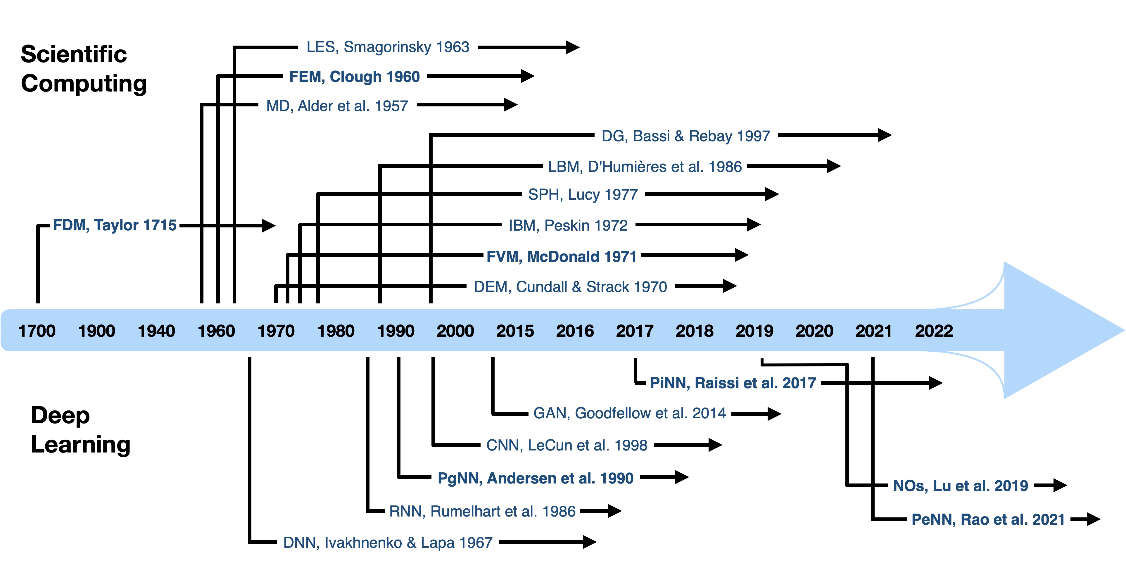
Figure 1: A schematic representation of the history of development, including only seminal works, for scientific computing and DL approaches. For scientific computing, the following are listed: Finite Difference Method (FDM) [23], Molecular Dynamics (MD) [24], Finite Element Method (FDM) [25], Large Eddy Simulation (LES) [26], Discrete Element Method (DEM) [27], Finite Volume Method (FVM) [28], Immersed Boundary Method (IBM) [29], Smoothed Particle Hydrodynamics (SPH) [30], Lattice Boltzmann Method (LBM) [31], and Discontinuous Galerkin (DG) [32]. For deep learning, the following are listed: Deep Neural Network (DNN) [33], Recurrent Neural Network (RNN) [34], Physics-guided Neural Network (PgNN) [35], Convolutional Neural Network (CNN) [36], Generative Adversarial Network (GAN) [37], Physics-informed Neural Network (PiNN) [38], Neural Operators (NOs) [39], and Physics-encoded Neural Network (PeNN) [40].

Due to the intrinsic architecture of conventional DL methods, their learning is limited to the scope of the datasets with which the training is conducted (e.g., specific boundary conditions, material types, spatiotemporal discretization, etc.), and inference cannot be successfully scoped under any unseen conditions (e.g., new geometries, new material types, new boundary conditions, etc.). Because the majority of the scientific fields are not (big) data-oriented domains and cannot provide comprehensive datasets that cover all possible conditions, these models trained based on sparse datasets are accelerated but not predictive [22]. Thus, it is logical to leverage the wealth of prior knowledge, the underlying physics, and domain expertise to further constrain these models while training on available, sparse data points. Neural networks (NNs) are better suited to digest physical-driven or knowledge-based constraints during training. Based on how the underlying physics is incorporated, the authors categorized neural network applications in scientific computing into three separate types: (i) physics-guided neural networks (PgNNs), (ii) physics-informed neural networks (PiNNs), and (iii) physics-encoded neural networks (PeNNs).

In PgNN-based models, off-the-shelf supervised DL techniques are used to construct surrogate mappings between formatted inputs and outputs that are generated using experiments and computations in a controlled setting and curated through extensive processes to ensure compliance with physics principles and fundamental rules [22]. Such models require a rich and sufficient dataset to be trained and used reliably. A PgNN-based model maps a set of inputs x to a related set of outputs y using an appropriate function F with unknown parameters w such that $\textbf{y}=F(\textbf{x};\textbf{w})$. By specifying a particular structure for F, a data-driven approach generally attempts to fine-tune the parameters w so that the overall error between true values, $\hat{\textbf{y}}$, and those from model predictions, y, is minimized [7]. For complex physical systems, the data is likely sparse due to the high cost of data acquisition [41]. The vast majority of state-of-the-art PgNNs lack robustness and fail to fulfill any guarantees of generalization (i.e., interpolation [38, 42] and extrapolation [43]). To remediate this issue, PiNNs have been introduced to perform supervised learning tasks while obeying given laws of physics in the form of general non-linear differential equations [44, 10, 45, 46, 6].

The PiNN-based models respect the physical laws by incorporating a weakly imposed loss function consisting of the residuals of physics equations and boundary constraints. They leverage automatic differentiation [47] to differentiate the neural network outputs with respect to their inputs (i.e., spatiotemporal coordinates and model parameters). By minimizing the loss function, the network can closely approximate the solution [48, 49]. As a result, PiNNs lay the groundwork for a new modeling and computation paradigm that enriches DL with long-standing achievements in mathematical physics [38, 44]. The PiNN models face a number of limitations relating to theoretical considerations (e.g., convergence and stability [50, 6, 51]) and implementation considerations (e.g., neural network design, boundary condition management, and optimization aspects) [40, 10]. In addition, in cases where the explicit form of differential equations governing the complex dynamics is not fully known a priori, PiNNs encounter serious limitations [52]. For such cases, another family of DL approaches known as physics-encoded neural networks (PeNN) has been proposed [40].

The PeNN-based models leverage advanced architectures to address issues with data sparsity and the lack of generalization encountered by both PgNNs and PiNNs models. PeNN-based models forcibly encode the known physics into their core architecture (e.g., NeuralODE [53]). By construction, PeNN-based models extend the learning capability of a neural network from instance learning (imposed by PgNN and PiNN architectures) to continuous learning [53]. The encoding mechanisms of the underlying physics in PeNNs are fundamentally different from those in PiNNs [54, 55], although they can be integrated to achieve the desired non-linearity of the model. In comparison to PgNNs and PiNNs, the neural networks generated by the PeNN paradigm offer better performance against data sparsity and model generalizability [40].

There is another family of supervised learning methods that do not fit well under PgNN, PiNN, and PeNN categories as defined above. These models, dubbed as neural operators, learn the underlying linear and nonlinear continuous operators, such as integrals and fractional Laplacians, using advanced architectures (e.g., DeepONet [39, 56]). The data-intensive learning procedure of a neural operator may resemble the PgNN-based models learning, as both enforce the physics of the problem using labeled input-output dataset pairs. However, a neural operator is very different from a PgNN-based model that lacks generalization properties due to under-parameterization. A neural operator can be combined with PiNN and PeNN methods to train a model that can learn complex non-linearity in physical systems with extremely high generalization accuracy [43]. The robustness of neural operators for applications requiring real-time inference is a distinguishing characteristic [57].

This review paper is primarily intended for the scientific computing community interested in the application of neural networks in computational fluid and solid mechanics. It discusses the general architectures, advantages, and limitations of PgNNs, PiNNs, PeNNs, and neural operators and reviews the most prominent applications of these methods in fluid and solid mechanics. The remainder of this work is structured as follows: In Section 2, the potential of PgNNs to accelerate scientific computing is discussed. Section 3 provides an overview of PiNNs and discusses their potential to advance PgNNs. In Section 4, several leading PeNN architectures to address critical limitations in PgNNs and PiNNs are discussed. Section 4 reviews the recent developments in neural operators. Finally, in Section 6, an outlook for future research directions is provided.

2 Physics-guided Neural Networks, PgNNs

PgNNs use off-the-shelf supervised DL models to statistically learn the known physics of a desired phenomenon by extracting features or attributes from training datasets obtained through well-controlled experiments and computations [58]. PgNNs consist of one or a combination of Multilayer Perceptron (MLP, alternatively called artificial neural networks, ANN, or deep neural networks, DNN, in different studies relevant to this review) [58], CNN [58], RNN [58], GAN [59], and graph neural networks (GRNN) [60]. Although GAN models are categorized as unsupervised learning, they can be classified as PgNNs, in the context of this paper, because their underlying training is framed as a supervised learning problem [59, 61]. A schematic representation of a sample PgNN architecture is illustrated in Fig. 2. Any physical problem includes a set of independent features or input features as $\textbf{x}=[{X_{1}},{X_{2}},{X_{3}},...,{X_{n}}]$ and a set of dependent variables or desired outputs as $\textbf{y}=[{Y_{1}},{Y_{2}},{Y_{3}},...,{Y_{n}}]$. The data describing this physical phenomenon can be generated by experimentation (e.g., sensor-based observation, etc.), closure laws (e.g., Fourier’s law, Darcy’s law, drag force, etc.), or the solution of governing ordinary differential equations (ODE) and/or partial differential equations (PDE), e.g., Burger’s equation, Navier-Stokes equations, etc. The dependent variables and independent features thus comply with physics principles, and the trained neural network is guided inherently by physics throughout training.

In PgNNs, the neurons in each layer are connected to the neurons in the next layer through a set of weights. The output of each node is obtained by applying an activation function (e.g., rectified linear unit (ReLU), Tanh, Sigmoid, Linear, etc.) to the weighted sum of the outputs of the neurons in the preceding layer plus an additional bias [62]. This procedure sequentially obtains the output of the neurons in each layer, starting with the input. This process is typically called forward propagation. A loss function (or, alternatively, a cost function) is subsequently defined and calculated in order to evaluate the accuracy of the prediction. Commonly used loss functions for regression are L1 [63] and mean-squared-error (MSE) [63]. The next step in training involves error backpropagation, which calculates the partial derivatives/gradients of the cost function with respect to weights and biases (i.e., $\theta$ as shown in Fig. 2). Finally, an optimization technique, such as gradient descent [64], stochastic gradient descent [64], or mini-batch gradient descent [64], is used to minimize the loss function and simultaneously compute and update $\theta$ parameters using the calculated gradients from the backpropagation procedure. The process is iterated until the desired level of accuracy is obtained for a PgNN.

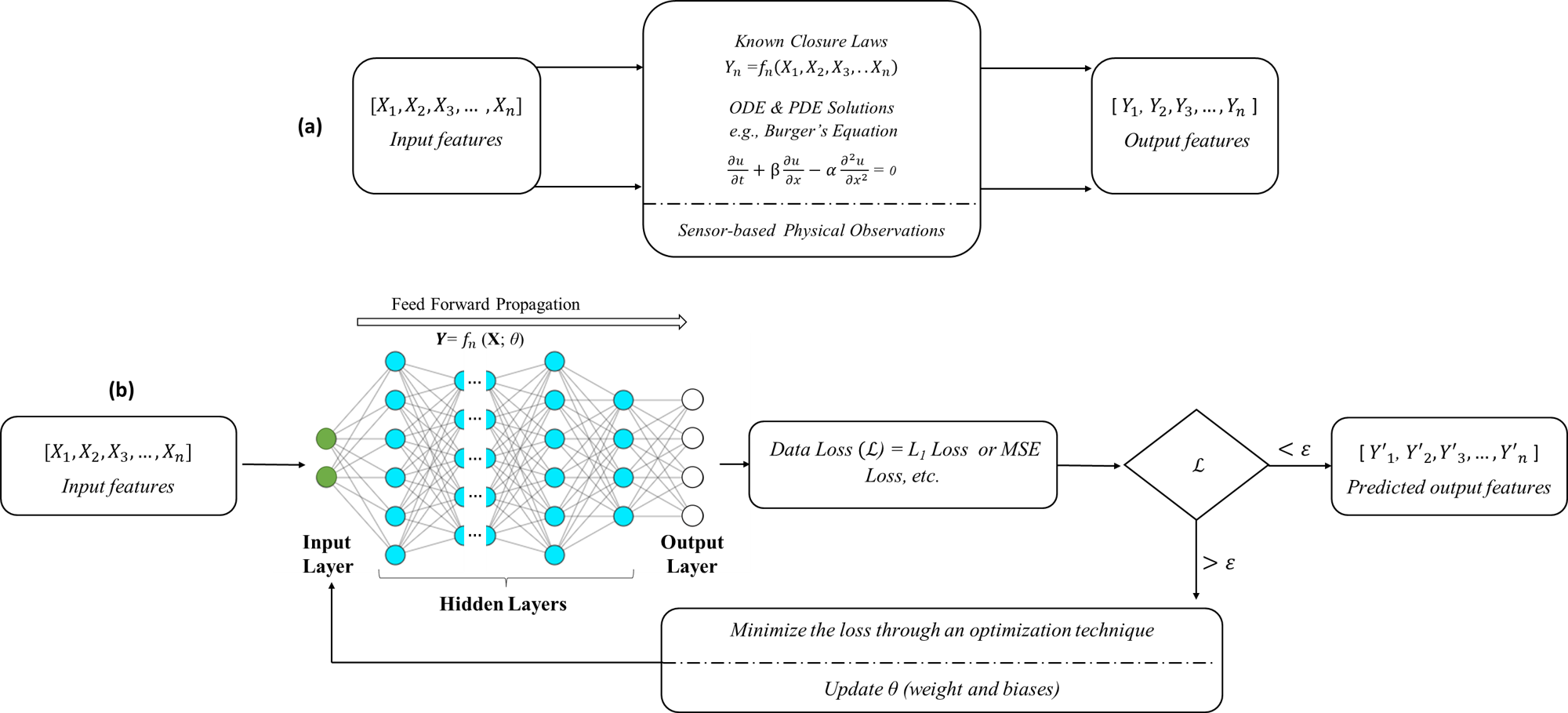
Figure 2: A schematic architecture of PgNNs. Panel (a) shows the typical generation of training datasets using known closure laws, direct numerical simulation of PDEs and ODEs, or experimentation to comply with physical principles. Panel (b) shows the architecture of a PgNN model consisting of a simple feed-forward neural network (which can be replaced with any other network type). The loss function made of $L_{1}$, $L_{2}$ regularization, MSE, or other user-defined error functions is minimized iteratively in the training phase. $\theta$ is the learnable parameter corresponding to weights/biases in the neural network that can be learned simultaneously while minimizing the loss function.

In recent years, PgNN has been extensively used to accelerate computational fluid dynamics (CFD) [65], computational solid mechanics [66], and multi-functional material designs [67]. It has been employed in all computationally expensive and time-consuming components of scientific computing, such as (i) pre-processing [68, 65, 69], e.g., mesh generation; (ii) discretization and modeling [70, 71, 72], e.g., Finite Difference (FDM), Finite Volume (FVM), Finite Element (FEM), Discrete Element Method (DEM), Molecular Dynamics (MD), etc.; and (iii) post-processing, e.g., output assimilation and visualization [73, 74, 75]. These studies are arranged (i) to train shallow networks on small datasets to replace a bottleneck (i.e., a computationally expensive step) in conventional forward numerical modeling, e.g., drag coefficient calculation in concentrated complex fluid flow modeling [22, 76, 77, 78, 79]; or (ii) to train relatively deep networks on larger datasets generated for a particular problem, e.g., targeted sequence design within the coarse-grained polymer genome [80]. These networks acknowledge the physical principles upon which the training data is generated and accelerate the simulation process [75, 22].

Although the training of PgNNs appears to be straightforward, generating the data by tackling the underlying physics for complex physical problems could require a substantial computational cost [6, 13]. Once trained, a PgNN can significantly accelerate the computation speed for the phenomena of interest. It is worth noting that while a PgNN model may achieve a good accuracy on the training set based on numerous attempts, it is more likely to memorize the trends, noise, and detail in the training set rather than intuitively comprehend the pattern in the dataset. This is one of the reasons that PgNNs lose their prediction ability when inferred/tested outside the scope of the training datasets. PgNNs’ overfitting can be mitigated in different ways [81, 82, 83] to enhance the predictability of the model within the scope of the training data. In the following subsections, we review the existing literature and highlight some of the most recent studies that applied PgNNs to accelerate different steps in scientific computing for applications in fluid and solid mechanics.

2.1 Pre-Processing

Pre-processing is often the most work-intensive component in scientific computing, regardless of the numerical model type (e.g., FEM, FDM, FVM, etc.). The main steps in this component are the disassembly of the domain into small, but finite, parts (i.e., mesh generation, evaluation, and optimization) and the upscaling and/or downscaling of the mesh properties to use a spatiotemporally coarse mesh while implicitly solving for unresolved fine-scale physics. These two steps are time-consuming and require expert-level knowledge; hence, they are potential candidates to be replaced by accelerated PgNN-based models.

2.1.1 Mesh Generation

Mesh generation is a critical step for numerical simulations. Zhang et al. [68] proposed the automatic generation of an unstructured mesh based on the prediction of the required local mesh density throughout the domain. For that purpose, an ANN was trained to guide a standard mesh generation algorithm. They also proposed extending the study to other architectures, such as CNN or GRNN, for future studies including larger datasets and/or higher-dimensional problems. Huang et al. [65] adopted a DL approach to identify optimal mesh densities. They generated optimized meshes using classical CFD tools (e.g., Simcenter STAR-CCM+ [84]) and proposed training a CNN to predict optimal mesh densities for arbitrary geometries. The addition of an adaptive mesh refinement version accelerated the overall process without compromising accuracy and resolution. The authors proposed learning optimal meshes (generated by corresponding solvers with adjoint functionality) using ANN, which may be utilized as a starting point in other simulation tools irrespective of the specific numerical approach [65]. Wu et al. [69] also proposed a mesh optimization method by integrating the moving mesh method with DL in order to solve the mesh optimization problem. With the experiments carried out, a neural network with high accuracy was constructed to optimize the mesh while preserving the specified number of nodes and topology of the initially given mesh. Using this technique, they also demonstrated that the moving mesh algorithm is independent of the CFD computation [69].

In mesh generation, a critical issue has been the evaluation of mesh quality due to a lack of general and effective criteria. Chen et al. [85] presented a benchmark dataset (i.e., the NACA-Market reference dataset) to facilitate the evaluation of a mesh’s quality. They presented GridNet, a technique that uses a deep CNN to perform an automatic evaluation of the mesh’s quality. This method receives the mesh as input and conducts the evaluation. The mesh quality evaluation using a deep CNN model trained on the NACA-Market dataset proved to be viable with an accuracy of 92.5 percent [85].

2.1.2 Cross-scaling Techniques

It is always desirable to numerically solve a multi-physics problem on a spatiotemporally coarser mesh to minimize computational cost. For this reason, different upscaling [86, 87], downscaling [88], and cross-scaling [89] methods have been developed to determine accurate numerical solutions to non-linear problems across a broad range of length- and time-scales. One viable choice is to use a coarse mesh that reliably depicts long-wavelength dynamics and accounts for unresolved small-scale physics. Deriving the mathematical model (e.g., boundary conditions) for coarse representations, on the other hand, is relatively hard. Bar-Sinai et al. [87] proposed a PgNN model for learning optimum PDE approximations based on actual solutions to known underlying equations. The ANN outputs spatial derivatives, which are then optimized in order to best satisfy the equations on a low-resolution grid. Compared to typical discretization methods (e.g., finite difference), the recommended ANN method was considerably more accurate while integrating the set of non-linear equations at a resolution that was 4 to 8 times coarser [87]. The main challenge in this approach, however, is to systematically derive these kinds of solution-adaptive discrete operators. Maddu et al. [86] developed a PgNN, dubbed as STENCIL-NET, for learning resolution-specific local discretization of non-linear PDEs. By combining spatially and temporally adaptive parametric pooling on regular Cartesian grids with knowledge about discrete time integration, STENCIL-NET can accomplish numerically stable discretization of the operators for any arbitrary non-linear PDE. The STENCIL-NET model can also be used to determine PDE solutions over a wider spatiotemporal scale than the training dataset. In their paper, the authors employed STENCIL-NET for long-term forecasting of chaotic PDE solutions on coarse spatiotemporal grids to test their hypothesis. Comparing the STENCIL-NET model to baseline numerical techniques (e.g., fully vectorized WENO [90]), the predictions on coarser grids were faster by up to 25 to 150 times on GPUs and 2 to 14 times on CPUs, while maintaining the same accuracy [86].

Table 1 reports a non-exhaustive list of recent works that leveraged PgNNs to accelerate the pre-processing part of scientific computing. These studies collectively concluded that PgNN can be successfully integrated to achieve a considerable speed-up factor in mesh generation, mesh evaluation, and cross-scaling, which are vital for many complex problems explored using scientific computing techniques. The next subsection discusses the potential of PgNN to be incorporated into the modeling components, hence yielding a higher speed-up factor or greater accuracy.

Table 1: A non-exhaustive list of recent studies that leveraged PgNNs to accelerate the pre-processing part in scientific computing.

Area of application	NN Type	Objective	Reference
Mesh Generation	ANN	Generating unstructured mesh	[68]
	CNN	Predicting meshes with optimal density and accelerating meshing process without compromising performance or resolution	[65]
	ANN	Generating high quality tetrahedral meshes	[91]
	ANN	Developing a mesh generator tool to produce high-quality FEM meshes	[92]
	ANN	Generating finite element mesh with less complexities	[93]
Mesh Evaluation	CNN	Conducting automatic mesh evaluation and quality assessment	[85]
Mesh Optimisation	ANN	Optimizing mesh while retaining the same number of nodes and topology as the initially given mesh	[69]
Cross-scaling	ANN	Utilizing data-driven discretization to estimate spatial derivatives that are tuned to best fulfill the equations on a low-resolution grid.	[87]
	ANN (STENCIL-NET)	Providing solution-adaptive discrete operators to predict PDE solutions on bigger spatial domains and for longer time frames than it was trained	[86]

2.2 Modeling and Post-processing

2.2.1 PgNNs for Fluid Mechanics

PgNN has gained considerable attention from the fluid mechanics’ community. The study by Lee and Chen [94] on estimating fluid properties using ANN was among the first studies that applied PgNN to fluid mechanics. Since then, the application of PgNNs in fluid mechanics has been extended to a wide range of applications, e.g., laminar and turbulent flows, non-Newtonian fluid flows, aerodynamics, etc., especially to speed up the traditional computational fluid dynamics (CFD) solvers.

For incompressible laminar flow simulations, the numerical procedure to solve Navier–Stokes equations is considered as the main bottleneck. To alleviate this issue, PgNNs have been used as a part of the resolution process. For example, Yang et al. [95] proposed a novel data-driven projection method using an ANN to avoid iterative computation of the projection step in grid-based fluid simulations. The efficiency of the proposed data-driven projection method was shown to be significant, especially in large-scale fluid flow simulations. Tompson et al. [96] used a CNN for predicting the numerical solutions to the inviscid Euler equations for fluid flows. An unsupervised training that incorporates multi-frame information was proposed to improve long-term stability. The CNN model produced very stable divergence-free velocity fields with improved accuracy when compared to the ones obtained by the commonly used Jacobi method [97]. Chen et al. [98] later developed a U-net-based architecture, a particular case of a CNN model, for the prediction of velocity and pressure field maps around arbitrary 2D shapes in laminar flows. The CNN model is trained with a dataset composed of random shapes constructed using Bézier curves and then by solving Navier-Stokes equations using a CFD solver. The predictive efficiency of the CNN model was also assessed on unseen shapes, using ad hoc error functions, specifically, the MSE levels for these predictions were found to be in the same order of magnitude as those obtained on the test subset, i.e., between $1.0\times 10^{-5}$ and $5.0\times 10^{-5}$ for both pressure and velocity, respectively.

Moving from laminar to turbulent flow regimes, PgNNs have been extensively used for the formulation of turbulence closure models [99]. Ling et al. [100] used a feed-forward MLP and a specialized neural network to predict Reynolds-averaged Navier–Stokes (RANS) and Large Eddy Simulation (LES) turbulence problems. Their specialized neural network embeds Galilean invariance [101] using a higher-order multiplicative layer. The performance of this model was compared with that of MLP and ground truth simulations. They concluded that the specialized neural network can predict the anisotropy tensor on an invariant tensor basis, resulting in significantly more accurate predictions than MLP. Maulik et al. [102] presented a closure framework for subgrid modeling of Kraichnan turbulence [103]. To determine the dynamic closure strength, the proposed framework used an implicit map with inputs as grid-resolved variables and eddy viscosities. Training an ANN with extremely subsampled data obtained from high-fidelity direct numerical simulations (DNSs) yields the optimal map. The ANN model was found to be successful in imbuing the decaying turbulence problem with dynamic kinetic energy dissipation, allowing accurate capture of coherent structures and inertial range fidelity. Later, Kim and Lee [104] used simple linear regression, SLinear, multiple linear regression, MLinear, and a CNN to predict the turbulent heat transfer (i.e., the wall-normal heat flux, $q_{w}$) using other wall information, including the streamwise wall-shear stress, spanwise wall-shear stress or streamwise vorticity, and pressure fluctuations, obtained by DNSs of a channel flow (see Fig. 3(a)). The constructed network was trained using adaptive moment estimation (ADAM) [105, 106], and the grid searching method [107, 108] was performed to optimize the depth and width of the CNN. Their finding showed that the PgNN model is less sensitive to the input resolution, indicating its potential as a good heat flux model in turbulent flow simulation. Yousif et al. [109] also proposed an efficient method for generating turbulent inflow conditions based on a PgNN formed by a combination of a multiscale convolutional auto-encoder with a subpixel convolution layer (MSCSP-AE) [110, 111] and long short-term memory (LSTM) [112, 113] model. The proposed model was found to have the capability to deal with the spatial mapping of turbulent flow fields.

PgNNs have also been applied in the field of aerodynamics. Kou and Zhang [114] presented a review paper on typical data-driven methods, including system identification, feature extraction, and data fusion, that have been employed to model unsteady aerodynamics. The efficacy of those data-driven methods is described by several benchmark cases in aeroelasticity. Wang et al. [115] described the application of ANN to the modeling of the swirling flow field in a combustor (see Fig. 3(b)). Swirling flow field data from particle image velocimetry (PIV) was used to train an ANN model. The trained PgNN model was successfully tested to predict the swirling flow field under unknown inlet conditions. Chowdhary et al. [116] studied the efficacy of combining ANN models with projection-based (PB) model reduction techniques [117, 118] to develop an ANN-surrogate model for computationally expensive, high-fidelity physics models, specifically for complex hypersonic turbulent flows. The surrogate model was used to perform Bayesian estimation of freestream conditions and parameters of the SST (shear stress transport) turbulence model. The surrogate model was then embedded in the high-fidelity (Reynolds-averaged Navier–Stokes) flow simulator, using shock-tunnel data. Siddiqui et al. [119] developed a non-linear data-driven model, encompassing Time Delay Neural Networks (TDNN), for a pitching wing. The pitch angle was considered as the input to the model, while the lift coefficient was considered as the output. The results showed that the trained models were able to capture the non-linear aerodynamic forces more accurately than linear and semi-empirical models, especially at higher offset angles. Wang et al. [120] also proposed a multi-fidelity reduced-order model based on multi-task learning ANNs to efficiently predict the unsteady aerodynamic performance of an iced airfoil. The results indicated that the proposed model achieves higher accuracy and better generalization capability compared with single-fidelity and single-task modeling approaches.

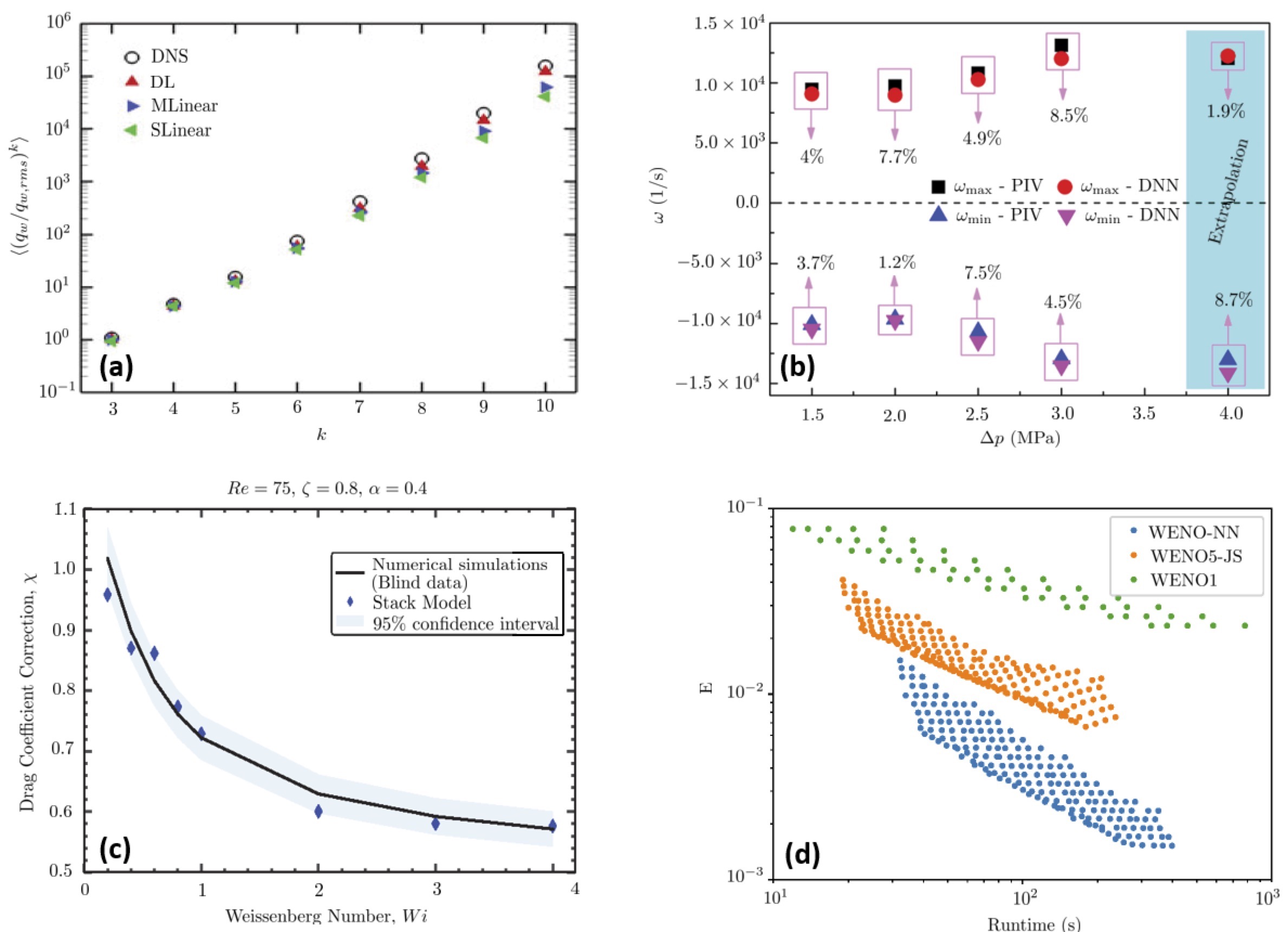
Figure 3: Panel (a) shows a comparison of the high-order moments of the heat flux data obtained from DNS of turbulent heat transfer and predictions obtained by SLinear, MLinear, and CNN (i.e., PgNN) models developed by Kim and Lee [104]. Notice that $q_{w,rms}$ is the root-mean-squared-error (RMSE) of $q_{w}$, $k$ denotes the index of the weights in the network and the angle bracket denotes the average over all test points. Panel (b) shows the comparison of a PgNN model and PIV technique for the prediction of the swirling flow field in a combustor [115]. The changes in maximum and minimum vorticity, $\omega$ (1/s), in a swirling flow field are shown for several pressure drops, $\Delta p$ (MPa). Panel (c) shows the performance of the PgNN model developed by Faroughi et al. [22] against the blind dataset generated to predict the drag coefficient of a spherical particle translating in a Giesekus fluid at Reynolds number $Re=75$, retardation ratio $\zeta=0.8$ and mobility parameter $\alpha=0.4$. Panel (d) shows a comparison of the $L_{2}^{2}$ error ($E$) and simulation run time of WENO-NN, weighted ENO-Jiang Shu (WENO5-JS) scheme convergent at fifth order, and weighted ENO (WENO1) scheme convergent at first order, to simulate shock wave interactions Stevens and Colonius [121].

The simulation of complex fluid flows, specifically using fluids that exhibit viscoelastic nature and non-linear rheological behaviors, is another topic where PgNNs have been applied [122, 123]. The dynamics of these fluids are generally governed by non-linear constitutive equations that lead to stiff numerical problems [124, 125]. Faroughi et al. [22] developed a PgNN model to predict the drag coefficient of a spherical particle translating in viscoelastic fluids (see Fig. 3(c)). The PgNN considered a stacking technique (i.e., ensembling Random Forrest [126], Extreme Gradient Boosting [127] and ANN models) to digest inputs (Reynolds number, Weissenberg number, viscosity ratio, and mobility factor considering both Oldroyd-B and Giesekus fluids) and outputs drag predictions based on the individual learner’s predictions and an ANN meta-regressor. The accuracy of the model was successfully checked against blind datasets generated by DNSs. Lennon et al. [128] also developed a tensor basis neural network (TBNN) allowing rheologists to construct learnable constitutive models that incorporate essential physical information while remaining agnostic to details regarding particular experimental protocols or flow kinematics. The TBNN model incorporates a universal approximator within a materially objective tensorial constitutive framework that, by construction, respects physical constraints, such as frame-invariance and tensor symmetry, required by continuum mechanics. Due to the embedded TBNN, the developed rheological universal differential equation quickly learns simple yet accurate and highly general models for describing the provided training data, allowing a rapid discovery of constitutive equations.

Lastly, PgNNs have also been extensively used to improve both the accuracy and speed of CFD solvers. Stevens and Colonius [121] developed a DL model (the weighted essentially non-oscillatory neural network, WENO-NN) to enhance a finite-volume method used to discretize PDEs with discontinuous solutions, such as the turbulence–shock wave interactions (see Fig. 3(d)). Kochkov et al. [18] used hybrid discretizations, combining CNNs and subcomponents of a numerical solver, to interpolate differential operators onto a coarse mesh with high accuracy. The training of the model was performed within a standard numerical method for solving the underlying PDEs as a differentiable program, and the method allows for end-to-end gradient-based optimization of the entire algorithm. The method learns accurate local operators for convective fluxes and residual terms and matches the accuracy of an advanced numerical solver running at 8 to 10 times finer resolution while performing the computation 40 to 80 times faster. Cai et al. [129] implemented a least-squares ReLU neural network (LSNN) for solving the linear advection-reaction problem with a discontinuous solution. They showed that the proposed method outperformed mesh-based numerical methods in terms of the number of DOFs (degrees of freedom). Haber et al. [130] suggested an auto-encoder CNN to reduce the resolution cost of a scalar transport equation coupled to the Navier–Stokes equations. Lara and Ferrer [131] proposed to accelerate high-order discontinuous Galerkin methods using neural networks. The methodology and bounds were examined for a variety of meshes, polynomial orders, and viscosity values for the 1D Burgers’ equation. List et al. [132] employed CNN to train turbulence models to improve under-resolved, low-resolution solutions to the incompressible Navier–Stokes equations at simulation time. The developed method consistently outperforms simulations with a two-fold higher resolution in both spatial and temporal dimensions. For mixing layer cases, the hybrid model on average resembles the performance of three-fold reference simulations, which corresponds to a speed-up of 7.0 times for the temporal layer and 3.7 times for the spatial mixing layer.

Table 2 reports a non-exhaustive list of recent studies that leveraged PgNN to model fluid flow problems. These studies collectively concluded that PgNNs can be successfully integrated with CFD solvers or used as standalone surrogate models to develop accurate and yet faster modeling components for scientific computing in fluid mechanics. In the next section, the potential application of PgNNs in computational solid mechanics is discussed.

Table 2: A non-exhaustive list of studies that leveraged PgNNs to model fluid computational flow problems.

Area of application	NN Type	Objective	Reference
Laminar Flows	CNN	Calculating numerical solutions to the inviscid Euler equations	[96]
	CNN	Predicting the velocity and pressure fields around arbitrary 2D shapes	[98]
Turbulent Flows	ANN	Developing a model for the Reynolds stress anisotropy tensor using high-fidelity simulation data	[100]
	ANN	Modelling of LESs of a turbulent plane jet flow configuration	[133]
	CNN	Designing and training artificial neural networks based on local convolution filters for LES	[134]
	ANN	Developing subgrid modelling of Kraichnan turbulence	[102]
	CNN	Estimating turbulent heat transfer based on other wall information acquired from channel flow DNSs	[104]
	CNN-LSTM	Generating turbulent inflow conditions with accurate statistics and spectra	[109]
Aerodynamics	CNN-MLP	Predicting incompressible laminar steady flow field over airfoils	[135]
	ANN	Developing a high-dimensional PgNN model for high Reynolds number turbulent flows around airfoils	[136]
	ANN	Modeling the swirling flow field in a combustor	[115]
	PCA-ANN	Creating surrogate models of computationally expensive, high-fidelity physics models for complex hypersonic turbulent flows	[116]
	ANN	Predicting unsteady aerodynamic performance of iced airfoil	[120]
Viscoelastic Flows	ANN	Predicting drag coefficient of a spherical particle translating in viscoelastic fluids	[22]
	ANN	Constructing learnable constitutive models using a universal approximator within a materially objective tensorial constitutive framework	[128]
Enhance CFD Solvers	ANN	Developing an improved finite-volume method for simulating PDEs with discontinuous solutions	[121]
	CNN	Interpolating differential operators onto a coarse mesh with high accuracy	[18]
	LSNN	Solving the linear advection-reaction problem with discontinuous solution	[129]
	CNN	Modeling the scalar transport equation to reduce the resolution cost of forced cooling of a hot workpiece in a confined environment	[130]
	CNN	Accelerating high order discontinuous Galerkin methods	[131]
	CNN	Developing turbulence model to improve under-resolved low-resolution solutions to the incompressible Navier–Stokes equations at simulation time	[132]

2.2.2 PgNNs for Solid Mechanics

Physics-guided neural networks (PgNNs) have also been extensively adopted by the computational solid mechanics’ community. The study by Andersen et al. [35] on welding modeling using ANN was among the first studies that applied PgNN to solid mechanics. Since then, the application of PgNN has been extended to a wide range of problems, e.g., structural analysis, topology optimization, inverse materials design and modeling, health condition assessment, etc., especially to speed up the traditional forward and inverse modeling methods in computational mechanics.

In the area of structural analysis, Tadesse et al. [137] proposed an ANN for predicting mid-span deflections of a composite bridge with flexible shear connectors. The ANN was tested on six different bridges, yielding a maximum root-mean-squared error (RMSE) of 3.79%, which can be negligible in practice. The authors also developed ANN-based close-form solutions to be used for rapid prediction of deflection in everyday design. Güneyisi et al. [138] employed ANN to develop a new formulation for the flexural overstrength factor for steel beams. They considered 141 experimental data samples with different cross-sectional typologies to train the model. The results showed a comparable training and testing accuracy of 99 percent, indicating that the ANN model provided a reliable tool to estimate beams’ over-strength. Hung et al. [139] leveraged ANN to predict the ultimate load factor of a non-linear, inelastic steel truss. They considered a planar 39-bar steel truss to demonstrate the efficiency of the proposed ANN. They used the cross-sections of members as the input and the load-factor as the output. The ANN-based model yielded a high degree of accuracy, with an average loss of less than 0.02, in predicting the ultimate load-factor of the non-linear inelastic steel truss. Chen et al. [140] also used ANN to solve a three-dimensional (3D) inverse problem of a collision between an elastoplastic hemispherical metal shell and a rigid impactor. The goal was to predict the position, velocity, and duration of the collision based on the shell’s permanent plastic deformation. For static and dynamic loading, the ANN model predicted the location, velocity, and collision duration with high accuracy. Hosseinpour et al. [141] used PgNN for buckling capacity assessment of castellated steel beams subjected to lateral-distortional buckling. As shown in Fig. 4(a), the ANN-based model provided higher accuracy than well-known design codes, such as AS4100 [142], AISC [143], and EC3 [144] for modeling and predicting the ultimate moment capacities.

Topology optimization of materials and meta-materials is yet another domain where PgNNs have been employed [145, 146]. Topology optimization is a technique that identifies the optimal materials placed inside a prescribed domain to achieve the optimal structural performance [147]. For example, Abueidda et al. [148] developed a CNN model that performs real-time topology optimization of linear and non-linear elastic materials under large and small deformations. The trained model can predict the optimal designs with great accuracy without the need for an iterative process scheme and with very low inference computation time. Yu et al. [149] suggested an integrated two-stage technique made up of a CNN-based encoder and decoder (as the first stage) and a conditional GAN (as the second stage) that allows for the determination of a near-optimal topological design. This integration resulted in a model that determines a near-optimal structure in terms of pixel values and compliance with considerably reduced computational time. Banga et al. [150] also proposed a 3D encoder-decoder CNN to speed up 3D topology optimization and determine the optimal computational strategy for its deployment. Their findings showed that the proposed model can reduce the overall computation time by 40% while achieving accuracy in the range of 96%. Li et al. [151] then presented a GAN-based non-iterative near-optimal topology optimizer for conductive heat transfer structures trained on black-and-white density distributions. A GAN for low resolution topology was combined with a super resolution generative adversarial network, SRGAN, [152, 153] for a high resolution topology solution in a two-stage hierarchical prediction-refinement pipeline. When compared to conventional topology optimization techniques, they showed this strategy has clear advantages in terms of computational cost and efficiency.

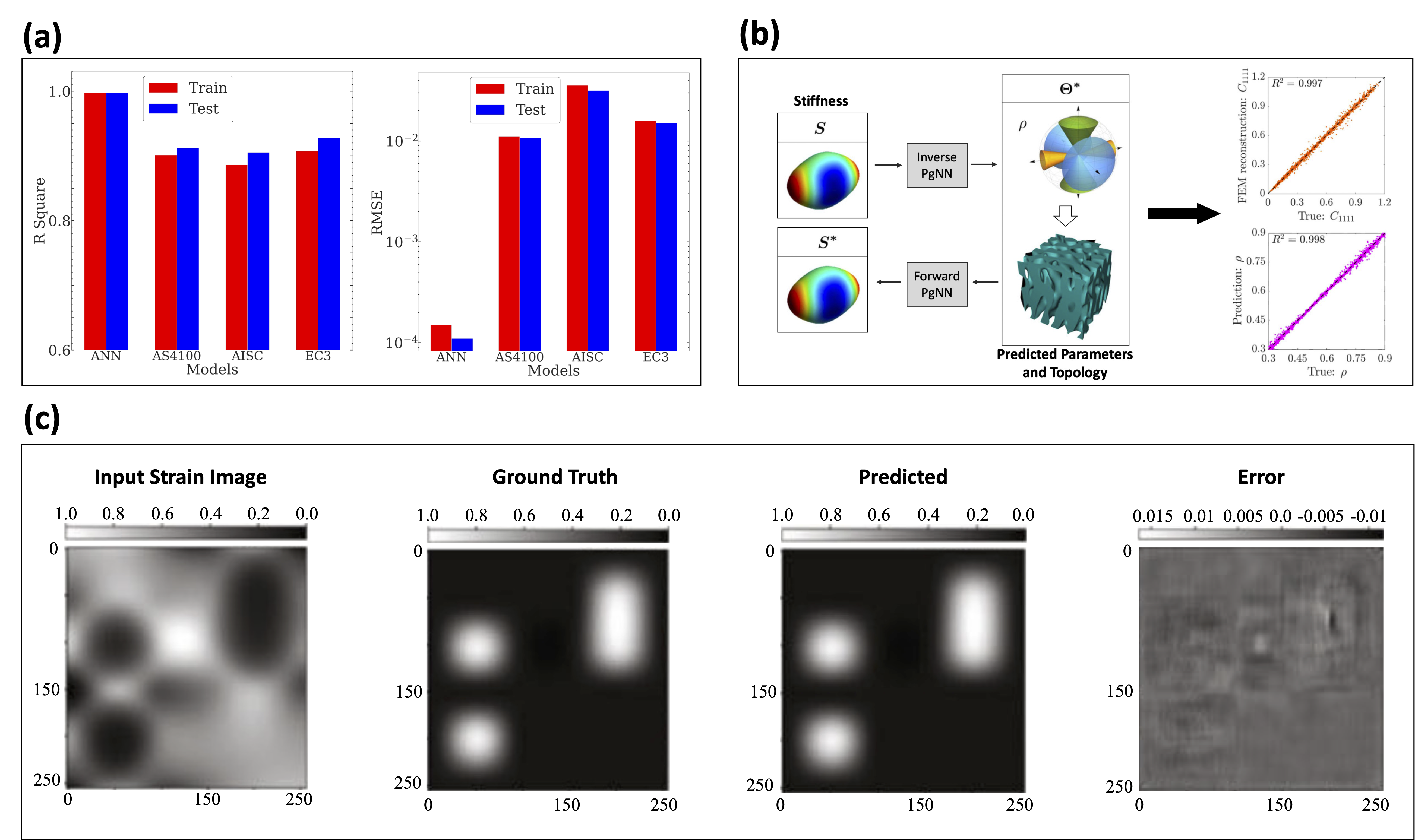
Figure 4: Panel (a) shows a comparison between ANN and other international codes’ accuracy (e.g., R-squared and RMSE) to predict the ultimate moment capacities of castellated beams subjected to lateral-distortional buckling (adapted from Hosseinpour et al. [141]). Panel (b) shows a two-stage PgNN architecture for predicting the design parameters of meta-materials for spindoid topologies. The first ANN (i.e., inverse PgNN) takes the query stiffness as input and outputs the design parameters. The second ANN (i.e., forward PgNN) takes the predicted design parameters and reconstructs the stiffness to verify inverse network accuracy. R-squared values for prediction of stiffness component $C_{1111}$ and design parameter $\rho$ are shown in the subsets (adapted from Kumar et al. [154]). Panel (c) shows a comparison between conditional GAN and ground truth made by elastography to predict elastic modulus from strain data (adapted from Ni and Gao [155]).

PgNN has also been applied for inverse design and modeling in solid mechanics. Messner [156] employed a CNN to develop surrogate models that estimate the effective mechanical properties of periodic composites. As an example, the CNN-based model was applied to solve the inverse design problem of finding structures with optimal mechanical properties. The surrogate models were in good agreement with well-established topology optimization methods, such as solid isotropic material with penalization (SIMP) [157], and were sufficiently accurate to recover optimal solutions for topology optimization. Lininger et al. [158] also used CNN to solve an inverse design problem for meta-materials made of thin film stacks. The authors demonstrated the CNN’s remarkable ability to explore the large global design space (up to 1012 parameter combinations) and resolve all relationships between meta-material structure and associated ellipsometric and reflectance/transmittance spectra [159, 158]. Kumar et al. [154] proposed a two-stage ANN model, as shown in Fig. 4(b), for inverse design of meta-materials. The model generates uniform and functionally graded cellular mechanical meta-materials with tailored anisotropic stiffness and density for spinodoid topologies. The ANN model used in this study is a combination of two-stage ANN, first ANN (i.e., inverse PgNN) takes query stiffness as input and outputs design parameters, e.g., $\Theta$. The second ANN (i.e., forward PgNN) takes the predicted design parameters as input and reconstructs the stiffness to verify the first ANN results. The prediction accuracy for stiffness and the design parameter was validated against ground truth data for both networks; sample comparisons and their corresponding R-squared values are shown in Fig. (4(b). Ni and Gao [155] proposed a combination of representative sampling spaces and conditional GAN, cGAN [160, 161], to address the inverse problem of modulus identification in the field of elasticity. They showed that the proposed approach can be deployed with high accuracy, as shown in Fig. 4(c) while avoiding the use of costly iterative solvers used in conventional methods, such as the adjoint weighted approach [162]. This model is especially suitable for real-time elastography and high-throughput non-destructive testing techniques used in geological exploration, quality control, composite material evaluation, etc.

The PgNN models have also been used to overcome some of the computational limitations of multiscale simulations in solid mechanics. This is achieved by (i) bypassing the costly lower-scale calculations and thereby speeding the macro-scale simulations [66], or (ii) replacing a step or the complete simulation with surrogate models [66]. For example, Liang et al. [163] developed an ANN model that takes finite element-based aorta geometry as input and output the aortic wall stress distribution directly, bypassing FEM calculation. The difference between the stress calculated by FEM and the one estimated by the PgNN model is practically negligible, while the PgNN model produces output in just a fraction of the FEM computational time. Mozaffar et al. [164] successfully employed RNN-based surrogate models for material modeling by learning the reversible, irreversible, and history-dependent phenomena that occur when studying material plasticity. Mianroodi et al. [2] used a CNN-based solver to predict the local stresses in heterogeneous solids with the highly non-linear material response and mechanical contrast features. When compared to common solvers like FEM, the CNN-based solver offered an acceleration factor of 8300x for elasto-plastic materials. Im et al. [5] proposed a PgNN framework to construct a surrogate model for a high-dimensional elasto-plastic FEM model by integrating an LSTM network with the proper orthogonal decomposition (POD) method [165, 166]. The suggested POD-LSTM surrogate model allows rapid, precise, and reliable predictions of elasto-plastic structures based on the provided training dataset exclusively. For the first time, Long et al. [167] used a CNN to estimate the stress intensity factor of planar cracks. Compared to FEM, the key benefit of the proposed light-weight CNN-based crack evaluation methodology is that it can be installed on an unmanned machine to automatically monitor the severity of a crack in real-time.

Table 3 reports a non-exhaustive list of recent studies that leveraged PgNNs in solid mechanics and materials design problems. These studies collectively concluded that PgNNs can be successfully integrated with conventional solvers (e.g., FEM solvers) or used as standalone surrogate models to develop accurate and yet faster modeling components for scientific computing in solid mechanics. Albeit, PgNNs come with their own limitations and shortcomings that might compromise solutions under different conditions, as discussed in the next section.

Table 3: A non-exhaustive list of studies that leveraged PgNNs to model solid mechanics problems.

Area of application	NN Type	Objective	Reference
Accelerating Simulations	ANN	Predicting the aortic wall stress distribution using FEM aorta geometry	[163]
	RNN	Developing surrogate models for material modeling by learning reversible, irreversible, and history-dependent phenomena	[164]
	CNN	Predicting local stresses in heterogeneous solids with the highly non-linear material response and mechanical contrast features	[2]
	CNN	Estimating stress intensity factor of planar cracks	[167]
Topology Optimization	CNN	Optimizing topology of linear and non-linear elastic materials under large and small deformations	[148]
	CNN-GAN	Determining near-optimal topological design	[149]
	CNN	Accelerating 3D topology optimization	[150]
	GAN-SRGAN	Generating near-optimal topologies for conductive heat transfer structures	[151]
Inverse Modeling	CNN	Estimating effective mechanical properties for periodic composites	[156]
	CNN	Solving an inverse design problem for meta-materials made of thin film stacks	[158]
	cGAN	Addressing inverse problem of modulus identification in elasticity	[155]
	CVAE	Designing nano-patterned power splitters for photonic integrated circuits	[155]
Structural Elements	ANN	Predicting non-linear buckling load of an imperfect reticulated shell	[168]
	ANN	Optimizing dynamic behavior of thin-walled laminated cylindrical shells	[169]
	ANN	Determining and identifying loading conditions for shell structures	[140]
Structural Analysis	CNN	Forecasting stress fields in 2D linear elastic cantilevered structures subjected to external static loads	[170]
	ANN	Estimating the thickness and length of reinforced walls based on previous architectural projects	[171]
Condition Assessment	Auto-encoder-NN	Learning mapping between vibration characteristics and structural damage	[172]
	CNN	Providing a real-time crack assessment method	[173]
	RNN	Nonparametric identification of large civil structures subjected to dynamic loadings	[174]
	CNN	Damage Identification of truss structures using noisy incomplete modal data	[175]

2.3 PgNNs Limitations

Even though PgNN-based models show great potential to accelerate the modeling of non-linear phenomena described by input-output interdependencies, they suffer from several critical limitations and shortcomings. Some of these limitations become more pronounced when the training datasets are sparse.

• The main PgNNs’ limitation stems from the fact that their training process is solely based on statistics [58]. Even though the training datasets are inherently constrained by physics (e.g., developed by direct numerical simulation, closure laws, and de-noised experimentation), PgNN generates models based on correlations in statistical variations. The outputs (predictions), thus, are naturally physics-agnostic [38, 176] and may violate the underlying physics [6].

• Another important limitation of PgNNs stems from the fact that training datasets are usually sparse, especially in the scientific fields discussed in this paper. When the training data is sparse and does not cover the entire range of underlying physiochemical attributes, the PgNN-based models fail in blind-testing on conditions outside the scope of training [43], i.e., they do not offer extrapolation capabilities in terms of spatiotemporal variables and/or other physical attributes.

• PgNN’s predictions might be severely compromised, even for inputs within the scope of sparse training datasets [22]. The lack of interpolation capabilities is more pronounced in complex and non-linear problems where the range of the physiochemical attributes is extremely wide (e.g., the range of Reynolds numbers from creeping flow to turbulent flow).

• PgNNs may not fully satisfy the initial conditions and boundary conditions using which the training datasets are generated [38]. The boundary conditions and computational domain vary from one problem to another, making the data generation and training process prohibitively costly. In addition, a significant portion of scientific computing research involves inverse problems in which unknown physiochemical attributes of interest are estimated from measurements or calculations that are only indirectly related to these attributes [177, 178, 10, 13]. For instance, in groundwater flow modeling, we leverage measurements of the pressure of a fluid immersed in an aquifer to estimate the aquifer’s geometry and/or material characteristics [179]. Such requirements further complicate the process of developing a simple neural network that is predictive under any conditions.

• PgNNs-based models are not resolution-invariant by construction [180], hence they cannot be trained on a lower resolution and be directly inferred on a higher resolution. This shortcoming is due to the fact that PgNN is only designed to learn the solution of physical phenomena for a single instance (i.e., inputs-outputs).

• Through the training process, PgNN-based networks learn the input-output interdependencies across the entire dataset. Such a process could potentially consider slight variations in the functional dependencies between different input and output pairs as noise, and produce an average solution. Consequently, while these models are optimal with respect to the entire dataset, they may produce suboptimal results in individual cases.

• PgNN models may struggle to learn the underlying process when the training dataset is diverse, i.e., when the interdependencies between different input and output pairs are drastically different. Although this issue can be mitigated by increasing the model size, more data is required to train such a network, making the training costly and, in some cases, impractical.

One way to resolve some of the PgNNs’ limitations is to generate more training data. However, this is not always a feasible solution due to the high cost of data acquisition. Alternatively, PgNNs can be further constrained by governing physical laws without any prior assumptions, reducing the need for large datasets. The latter is a plausible solution because, in most cases, the physical phenomenon can be fully and partially described using explicit ODEs, PDEs, and/or closure laws. This approach led to the development of a physics-informed neural network [38, 44], which is described and reviewed in the next section.

3 Physics-informed Neural Networks, PiNNs

In scientific computing, physical phenomena are often described using a strong mathematical form consisting of governing differential equations as well as initial and boundary conditions. At each point inside a domain, the strong form specifies the constraints that a solution must meet. The governing equations are usually linear or non-linear PDEs and/or ODEs. Some of the PDEs are notoriously challenging to solve, e.g., the Navier-Stokes equations to explain a wide range of fluid flows [10], Föppl–von Kármán equations to describe large deflections in solids [181, 181], etc. Other important PDE examples are heat equations [182], wave equation [183], Burgers’ equation [184], Laplace’s equation [185], Poisson’s equation [186], amongst others. This wealth of well-tested knowledge can be logically leveraged to further constrain PgNNs while training on available data points if any [38]. To this end, mesh-free physics-informed neural networks (PiNNs) have been developed [38, 44], quickly extended [187, 188], and extensively deployed in a variety of scientific and applied fields [189, 190, 191, 192, 193, 194]. Readers are referred to Karniadakis et al. [6] and Cai et al. [10] for the foundational review on how PiNNs function. This section briefly reviews the PiNN’s core architecture and its state-of-the-art applications in computational fluid and solid mechanics and discusses some of the major limitations.

A schematic representation of a vanilla PiNN architecture is illustrated in Fig. 5. In PiNNs, the underlying physics is incorporated outside the neural network architecture to constrain the model while training, thereby ensuring outputs follow known physical laws. The most common method to emulate this process is through a weakly imposed penalty loss that penalizes the network for not following the physical constraints. As shown in Fig. 5, a neural network with spatiotemporal features (i.e., x and $t$) as input parameters and the PDE solution elements as output parameters (i.e., u) can be used to emulate any PDE.

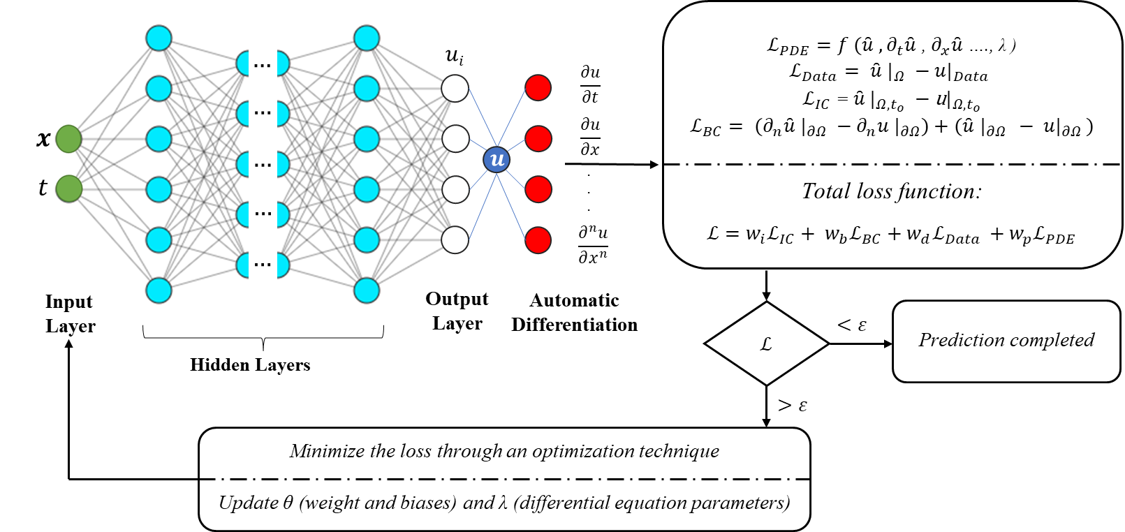
Figure 5: A schematic architecture of Physics-informed Neural Networks (PiNNs). The network digests spatiotemporal coordinates (x,t) as inputs to approximate the multi-physics solution $\hat{\textbf{{u}}}$. The last layer generates the derivatives of the predicted solution u with respect to inputs, which are calculated using automatic differentiation (AD). These derivatives are used to formulate the residuals of the governing equations in the loss function, which is composed of multiple terms weighted by different coefficients. $\theta$ and $\lambda$ are the learnable parameters for weights/biases and unknown PDE parameters, respectively, that can be learned simultaneously while minimizing the loss function.

The network’s outputs are then fed into the next layer, which is an automated differentiation layer. In this instance, multiple partial derivatives are generated by differentiating the outputs with regard to the input parameters (x and $t$). With the goal of optimizing the PDE solution, these partial derivatives are used to generate the required terms in the loss function. The loss function in PiNN is a combination of the loss owing to labelled data ($\mathcal{L}_{Data}$), governing PDEs ($\mathcal{L}_{PDE}$), applied initial conditions ($\mathcal{L}_{IC}$) and applied boundary conditions ($\mathcal{L}_{BC}$) [10]. The $\mathcal{L}_{BC}$ ensures that the PiNN’s solution meets the specified boundary constraints, whereas $\mathcal{L}_{Data}$ assures that the PiNN follows the trend in the training dataset (i.e., historical data, if any). Furthermore, the structure of the PDE is enforced in PiNN through the $\mathcal{L}_{PDE}$, which specifies the collocation points where the solution to the PDE holds [38]. The weights for the loss due to the initial conditions, boundary conditions, data, and PDE can be specified as $w_{i}$, $w_{b}$, $w_{d}$, and $w_{p}$, respectively. The next step is to check, for a given iteration, if the loss is within the accepted tolerance, $\epsilon$. If not, the learnable parameters of the network ($\theta$) and unknown PDE parameters ($\lambda$) are updated through error backpropagation. For a given number of iterations, the entire cycle is repeated until the PiNN model produces learnable parameters with loss functions less than $\epsilon$. Note that the training of PiNNs is more complicated compared to PgNNs, as PiNNs are composed of sophisticated non-convex and multi-objective loss functions that may result in instability during optimization [38, 6, 10].

Dissanayake and Phan-Thien [195] were the first to investigate the incorporation of prior knowledge into a neural network. Subsequently, Owhadi [196] introduced the concept of physics-informed learning models as a result of the ever-increasing computing power, which enables the use of increasingly complex networks with more learnable parameters and layers. The PiNN, as a new computing paradigm for both forward and inverse modeling, was introduced by Raissi et al. in a series of papers [38, 197, 44]. Raissi et al. [38] deployed two PiNN models, a continuous and a discrete-time model, on examples consisting of different boundary conditions, critical non-linearities, and complex-valued solutions such as Burgers’, Schrodinger’s, and Allen-Cahn’s equations. The results for Burgers’ equation demonstrated that, given a sufficient number of collocation points (i.e., as the basis for the continuous model), an accurate and data-efficient learning procedure can be obtained [38].

In continuous PiNN models, when dealing with higher-dimensional problems, the number of collocation points increases exponentially, making learning processing difficult and computationally expensive [38, 6]. Raissi et al. [38] presented a discrete time model based on the Runge-Kutta technique [198] to address the computational cost issue. This model simply takes a spatial feature as input, and over time steps, PiNN converges to the underlying physics. For all the examples explored by Raissi et al. [38], continuous and discrete PiNN models were able to satisfactorily build physics-informed surrogate models. Nabian et al. [199] proposed an alternate method for managing collocation points. They investigated the effect of sampling collocation points according to distribution and discovered that it was proportional to the loss function. This concept requires no additional hyperparameters and is simpler to deploy in existing PiNN models. In their study, they claimed that a sampling approach for collocation points enhanced the PiNN model’s behavior during training. The results were validated by deploying the hypothesis on PDEs for solving problems related to elasticity, diffusion, and plane stress physics.

In order to use PiNN to handle inverse problems, the loss function of the deep neural network must satisfy both the measured and unknown values at a collection of collocation sites distributed throughout the problem domain. Raissi et al. [44] showcased the potential of both continuous and discrete time PiNN models to solve benchmark inverse problems such as the propagation of non-linear shallow-water waves (Korteweg–De Vries equation) [200] and incompressible fluid flows (Navier-Stokes equations) [201].

Compared to PgNNs, the PiNN models provide more accurate predictions for forward and inverse modeling, particularly in scenarios with high non-linearities, limited data, or noisy data [202]. As a result, it has been implemented in several fundamental scientific and applied fields. Aside from forward and inverse problems, the PiNN can also be used to develop partial differential equations for unknown phenomena if training data representing the phenomenon’s underlying physics is available [44]. Raissi et al. [44] leveraged both continuous time and discrete time PiNN models for generating universal PDEs depending on the type and structure of the available data. In the remainder of this section, we review the recent literature on PiNN’s applications in the computational fluid and solid mechanics fields.

3.1 PiNNs for Fluid Mechanics

The application of PiNNs to problems involving fluid flow is an active, ongoing field of study [203, 204]. Raissi et al. [197], in a seminal work, developed a PiNN, so-called hidden fluid mechanics (HFM), to encode physical laws governing fluid motions, i.e., Navier-Stokes equations. They employed underlying conservation laws to derive hidden quantities of interest such as velocity and pressure fields from spatiotemporal visualizations of a passive scalar concentration, e.g., dye, transported in arbitrarily complex domains. Their algorithm to solve the data assimilation problem is agnostic to the boundary and initial conditions as well as to the geometry. Their model successfully predicted 2D and 3D pressure and velocity fields in benchmark problems inspired by real-world applications. Figure 6, adapted from Raissi et al. [197], compares the PiNN prediction with the ground truth for the classical problem of a 2D flow past a cylinder. The model can be used to extract valuable quantitative information such as wall shear stresses and lift and drag forces for which direct measurements are difficult to obtain.

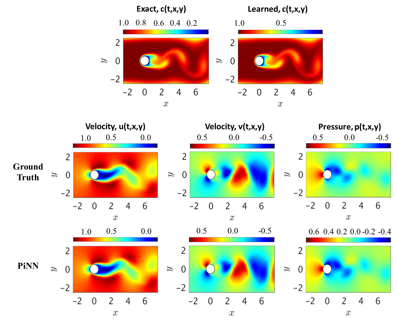
Figure 6: A comparison between ground truth simulation results and PiNN predictions for a 2D flow past a circular cylinder. Comparisons are shown for the concentration of passive scalar, $c(t,x,y)$, and resulting velocity fields, u,v, and pressure field, p (adapted from Raissi et al. [197]).

Zhang et al. [205] also developed a PiNN framework for the incompressible fluid flow past a cylinder governed by Navier-Stokes equations. PiNN learns the relationship between simulation output (i.e., velocity and pressure) and the underlying geometry, boundary, initial conditions, and inherently fluid properties. They demonstrated that the generalization performance is enhanced across both the temporal domain and design space by including Fourier features [206], such as frequency and phase offset parameters. Cheng and Zhang [207] developed Res-PiNN (i.e., Resnet blocks along with PiNN) for simulating cavity flow and flow past a cylinder governed by Burgers’ and Navier-Stokes equations. Their results showed that Res-PiNN had better predictive ability than conventional PgNN and vanilla PiNN algorithms. Lou et al. [208] also demonstrated the potential of PiNN for solving inverse multiscale flow problems. They used PiNN for inverse modeling in both the continuum and rare-field regimes represented by the Boltzmann-Bhatnagar-Gross-Krook (BGK) collision model. The results showed that PiNN-BGK is a unified method (i.e., it can be used for forward and inverse modeling), easy to implement, and effective in solving ill-posed inverse problems [208].

Wessels et al. [209] employed PiNN to develop an updated Lagrangian method for the solution of incompressible free surface flow subject to the inviscid Euler equations, the so-called Neural Particle Method (NPM). The method does not require any specific algorithmic treatment, which is usually necessary to accurately resolve the incompressibility constraint. In their work, it was demonstrated that NPM is able to accurately compute a pressure field that satisfies the incompressibility condition while avoiding topological constraints on the discretization process [209]. In addition, PiNN has also been employed to model complex non-Newtonian fluid flows involving non-linear constitutive PDEs able to characterize the fluid’s rheological behavior [210].

Haghighat et al. [211] trained a PiNN model to solve the dimensionless form of the governing equations of coupled multiphase flow and deformation in porous media. Almajid and Abu-Al-Saud [212] compared the predictions of PiNN with those of PgNN, i.e., a conventional artificial neural network, for solving the gas drainage problem of water-filled porous media. The study showed that PgNN performs well under certain conditions (i.e., when the observed data consists of early and late time saturation profiles), while the PiNN model performs robustly even when the observed data contains only an early time saturation profile (where extrapolations are needed). Depina et al. [213] applied PiNN to model unsaturated groundwater flow problems governed by the Richards PDE and van Genuchten constitutive model [214]. They demonstrated that PiNNs can efficiently estimate the van Genuchten model parameters and solve the inverse problem with a relatively accurate approximation of the solution to the Richards equation.

Some of the other variants of PiNN models employed in fluid mechanics are: nn-PiNN, where PiNN is employed to solve constitutive models in conjunction with conservation of mass and momentum for non-Newtonian fluids [210]; ViscoelasticNet, where PiNN is used for stress discovery and viscoelastic flow models selection [215], such as Oldroyd-B [124], Giesekus and Linear PTT [216]; RhINN which is a rheology-informed neural networks employed to solve constitutive equations for a Thixotropic-Elasto-Visco-Plastic complex fluid for a series of flow protocols [189]; CAN-PiNN, which is a coupled-automatic-numerical differential framework that combines the benefits of numerical differentiation (ND) and automatic differentiation (AD) for robust and efficient training of PiNN [217]; ModalPiNN, which is a combination of PiNN with enforced truncated Fourier decomposition [218] for periodic flow reconstruction [219]; GAPiNN, which is a geometry aware PiNN consisted of variational auto encoder, PiNN and boundary constraining network for real-world applications with irregular geometries without parameterization [220]; Spline-PiNN, which is a combination of PiNN and Hermite spline kernels based CNN employed to train a PiNN without any pre-computed training data and provide fast, continuous solutions that generalize to unseen domains [221]; cPiNN, which is a conservative physics-informed neural network consisting of several PiNNs communicating through the sub-domain interfaces flux continuity for solving conservation laws [187]; SA-PiNN, which is a self-adaptive PiNN to address the adaptive procedures needed to force PiNN to fit accurately the stubborn spots in the solution of stiff PDEs [50]; and XPiNN, which is an extended PiNN to enhance the representation and parallelization capacity of PiNN and generalization to any type of PDEs with respect to cPINN [188].

Table 4 reports a non-exhaustive list of recent studies that leveraged PiNN to model fluid flow problems. Furthermore, Table 5 reports a non-exhaustive list of recent studies that developed other variants of PiNN architectures to improve the overall prediction accuracy and computational cost in fluid flow problems.

Table 4: A non-exhaustive list of recent studies that leveraged PiNN to model fluid flow problems.

Area of Application	Objectives	Reference
Incompressible Flows	Accelerating the modeling of Navier-Stokes equations to infer the solution for various 2D and 3D flow problems	[44]
	Learning the relationship between output and underlying geometry as well as boundary conditions	[205]
	Simulating ill-posed (e.g., lacking boundary conditions) or inverse laminar and turbulent flow problems	[222]
Turbulent Flows	Solving vortex-induced and wake-induced vibration of a cylinder at high Reynolds number	[223]
	Simulating turbulent incompressible flows without using any specific model or making turbulence assumptions	[224]
	Reconstructing Reynolds stress disparities described by Reynolds-averaged Navier-Stokes equations	[225]
Geofluid Flows	Solving well-based groundwater flow equations without utilizing labeled data	[226]
	Predicting high-fidelity multi-physics data from low-fidelity fluid flow and transport phenomena in porous media	[227]
	Estimating Darcy’s law-governed hydraulic conductivity for both saturated and unsaturated flows	[228]
	Solving solute transport problems in homogeneous and heterogeneous porous media governed by the advection-dispersion equation	[49]
	Predicting fluid flow in porous media by sparse observations and physics-informed PointNet	[229]
Non-Newtonian Flows	Solving systems of coupled PDEs adopted for non-Newtonian fluid flow modeling	[210]
	Simulating linear viscoelastic flow models such as Oldroyd-B, Giesekus, and Linear PTT	[215]
	Simulating direct and inverse solutions of rheological constitutive models for complex fluids	[189]
Biomedical Flows	Enabling the seamless synthesis of non-invasive in-vivo measurement techniques and computational flow dynamics models derived from first physical principles	[230]
	Enhancing the quantification of near-wall blood flow and wall shear stress arterial in diseased arterial flows	[231]
Supersonic Flows	Solving inverse supersonic flow problems involving expansion and compression waves	[204]
Surface Water Flows	Solving ill-posed strongly non-linear and weakly-dispersive surface water waves governed by Serre-Green-Naghdi equations using only data of the free surface elevation and depth of the water.	[232]

Table 5: A non-exhaustive list of different variants of PiNN architectures used in modeling computational fluid flow problems.

PiNN Structure	Objective	Reference
CAN-PiNN	Providing a PiNN with more accuracy and efficient training by integrating ND- and AD-based approaches	[217]
ModalPiNN	Providing a simpler representation of PiNN for oscillating phenomena to improve performance with respect to sparsity, noise and lack of synchronization in the data	[219]
GA-PiNN	Enhancing PiNN to develop a parameter-free, irregular geometry-based surrogate model for fluid flow modeling	[220]
Spline-PiNN	Improving the generalization of PiNN by combining it with Hermite splines CNN to solve the incompressible Navier-Stokes equations	[221]
cPiNN	Enhancing PiNN to solve high dimensional non-linear conservation laws requiring high computational and memory requirements	[187]
SA-PiNN	Improving the PiNN’s convergence and accuracy problem for stiff PDEs using self-adaptive weights in the training	[50]
XPiNN	Improving PiNN and cPiNN in terms of generalization, representation, parallelization capacity, and computational cost	[188]
PiPN	overcoming the shortcoming of regular PiNNs that need to be retrained for any single domain with a new geometry	[233]

3.2 PiNNs for Solid Mechanics

The application of PiNNs in computational solid mechanics is also an active field of study. The study by Haghighat et al. [234] on modeling linear elasticity using PiNN was among the first papers that introduced PiNN in the solid mechanics community. Since then, the framework has been extended to other solid-mechanics problems (e.g., linear and non-linear elastoplasticity, etc.).

Shukla et al. [235] used PiNN for surrogate modeling of the micro-structural properties of poly-crystalline nickel. In their study, in addition to employing the PiNN model, they applied an adaptive activation function to accelerate the convergence of numerical modeling. The resulting PiNN-based surrogate model demonstrated a viable strategy for non-destructive material evaluation. Henkes et al. [236] modeled non-linear stress and displacement fields induced by inhomogeneities in materials with sharp phase transitions using PiNN. To overcome the PiNN’s convergence issues in this problem, they used adaptive training approaches and domain decomposition [209]. According to their results, the domain decomposition approach is capable of properly resolving non-linear stress, displacement, and energy in heterogeneous microstructures derived from real-world $\mu$CT-scans images [236]. Zhang and Gu [237] trained a PiNN model with a loss function based on the minimal energy criteria to investigate digital materials. The model tested on 1D tension, 1D bending, and 2D tensile problems demonstrated equivalent performance when compared to supervised DL methods (i.e., PgNNs). By adding a hinge loss for the Jacobian matrix, the PiNN method was able to properly approximate the logarithmic strain and rectify any erroneous deformation gradient.

Rao et al. [238] proposed a PiNN architecture with mixed-variable (displacement and stress component) outputs to handle elastodynamic problems without labeled data. The method was found to boost the network’s accuracy and trainability in contrast to the pure displacement-based PiNN model. Figure 7 compares the ground truth stress fields generated by the FEM with the ones estimated by mixed-variable PiNN for an elastodynamic problem [238]. It can be observed that stress components can be accurately estimated by mixed-variable PiNN. Rao et al. [238] also proposed a composite scheme of PiNN to enforce the initial and boundary conditions in a hard manner as opposed to the conventional (vanilla) PiNN with soft initial and boundary condition enforcement. This model was tested on a series of dynamics problems (e.g., the defected plate under cyclic uni-axial tension and elastic wave propagation), and resulted in the mitigation of inaccuracies near the boundaries encountered by PiNN.

Fang and Zhan [239] proposed a PiNN model to design the electromagnetic meta-materials used in various practical applications such as cloaking, rotators, concentrators, etc. They studied PiNN’s inference issues for Maxwell’s equation [240] with a high wave number in the frequency domain and improved the activation function to overcome the high wave number problems. The proposed PiNN recovers not only the continuous functions but also piecewise functions, which is a new contribution to the application of PiNN in practical problems. Zhang et al. [241] employed PiNN to identify nonhomogenous materials in elastic imaging for application in soft tissues. Two PiNNs were used, one for the approximate solution of the forward problem and another for approximating the field of the unknown material parameters. The results showed that the unknown distribution of mechanical properties can be accurately recovered using PiNN. Abueidda et al. [242] employed PiNN to simulate 3D hyperelasticity problems. They proposed an Enhanced-PiNN architecture consisting of the residuals of the strong form and the potential energy [243], producing several loss terms contributing to the definition of the total loss function to be minimized. The enhanced PiNN outperformed both the conventional (vanilla) PiNN and deep energy methods, especially when there were areas of high solution gradients.

Haghighat et al. [13] tested a different variant of PiNN to handle inverse problems and surrogate modeling in solid mechanics. Instead of employing a single neural network, they implemented a PiNN with multiple neural networks in their study. They deployed the framework on linear elastostatic and non-linear elastoplasticity problems and showed that the improved PiNN model provides a more reliable representation of the physical parameters. In addition, they investigated the domain of transfer learning in PiNN and found that the training phase converges more rapidly when transfer learning is used. Yuan et al. [244] proposed an auxiliary PiNN model (dubbed as A-PiNN) to solve inverse problems of non-linear integro-differential equations (IDEs). A-PiNNs circumvent the limitation of integral discretization by establishing auxiliary output variables in the governing equation to represent the integral(s) and by substituting the integral operator with automated differentiation of the auxiliary output. Therefore, A-PiNN, with its multi-output neural network, is constructed such that it determines both primary and auxiliary outputs to approximate both the variables and integrals in the governing equations. The A-PiNNs were used to address the inverse issue of non-linear IDEs, including the Volterra equation [245]. As demonstrated by their findings, the unknown parameters can be determined satisfactorily even with noisy data.

Some of the other variants of PiNN used in computational solid mechanics are: PhySRNet, which is a PiNN-based super-resolution framework for reconstructing high resolution output fields from low resolution counterparts without requiring high-resolution labelled data [246]; PDDO-PiNN, which is a combination of peridynamic differential operator (PDDO) [247] and PiNN to overcome degrading performance of PiNN under sharp gradients [248]; PiELM, which is a combination of PiNN and extreme learning machine (ELM) [249] employed to solve direct problems in linear elasticity [250]; DPiNN, which is a distributed PiNN utilizing a piecewise-neural network representation for the underlying field, instead of the piece-polynomial representation commonly used in FEM [51]; and PiNN-FEM, which is a mixed formulation based on PiNN and FE for computational mechanics in heterogeneous domain [251].

Table 6 reports a non-exhaustive list of recent studies that leveraged PiNN in computational solid mechanics. Furthermore, Table 7 reports a non-exhaustive list of recent studies that developed other variants of PiNN architectures to improve overall prediction accuracy and computational cost in solid mechanics modeling.

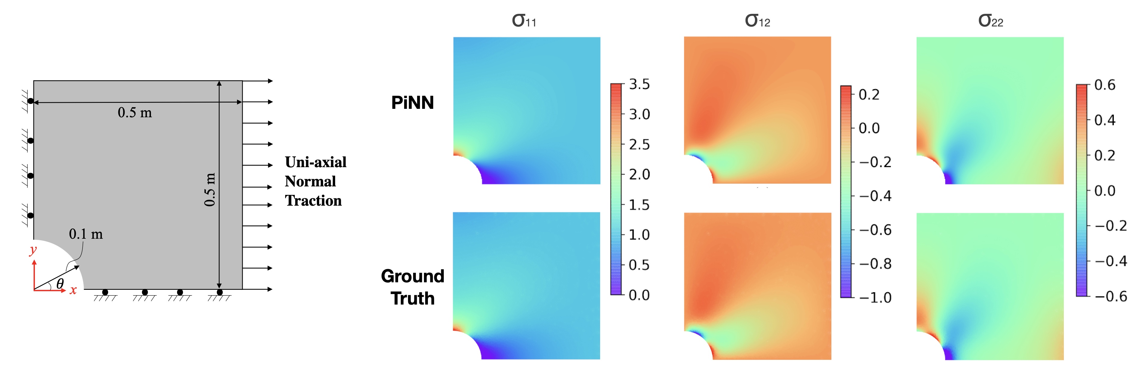
Figure 7: A comparison between mixed-variable PiNN’s prediction and ground truth generated by FEM to predict the stress fields in a defected plate under uni-axial load (adapted from Rao et al. [238]).

Table 6: A non-exhaustive list of recent studies that leveraged PiNN in computational solid mechanics.

Area of Application	Objectives	Reference
Elasticity	Solving forward and inverse problems in linear elastostatic and non-linear elasticity problems	[13]
	Simulating forward and discovery problems for linear elasticity	[234]
	Resolving the non-homogeneous material identification problem in elasticity imaging	[241]
	Estimating elastic properties of tissues using pre- and post-compression images of objects mimicking properties of tissues	[252]
	Estimating mechanical response of elastic plates under different loading conditions	[253]
	Finding optimal solutions to reference biharmonic problems of elasticity and elastic plate theory	[254]
	Simulating elastodynamic problems, e.g., elastic wave propagation, deflected plate under periodic uniaxial strain, without labeled data	[238]
Heterogeneous Materials	Inferring the spatial variation of compliance coefficients of materials (e.g., speed of the elastic waves) to identify microstructure	[235]
	Resolving non-linear stress, displacement, and energy fields in heterogeneous microstructures	[236]
	Solving coupled thermo-mechanics problems in composite materials	[255]
	Predicting the size, shape, and location of the internal structures (e.g., void, inclusion) using linear elasticity, hyperelasticity, and plasticity constitutive models	[256]
Structural Elements	Predicting the small-strain response of arbitrarily curved shells	[257]
	Solving mechanical problems of elasticity in one-dimensional elements such as rods and beams	[190]
	Predicting creep-fatigue life of components (316 stainless steel) at elevated temperatures	[258]
Structural Vibrations	Estimating and optimizing vibration characteristics and system properties of structural mechanics and vibration problems	[259]
Digital Materials	Resolving physical behaviors of digital materials to design next-generation composites	[237]
Fracture Mechanics	Reconstructing the solution of displacement field after damage to predict crack propagation for quasi-brittle materials	[260]
Elasto-viscoplasticity	Modeling the strain-rate and temperature dependence of the deformation fields (i.e., displacement, stress, plastic strain)	[261]
Additive Manufacturing	Predicting finite fatigue life in materials containing defects	[191]
Solid Mechanics	Providing a detailed introduction to programming PiNN-based computational solid mechanics from 1D to 3D problems	[262]

Table 7: A non-exhaustive list of different variants of PiNN architectures used in computational solid mechanics problems.

PiNN Architecture	Objectives	Reference
PhySRNet	Enhancing PiNN using super resolution techniques to reconstruct downscaled fields from their upscaled counterparts	[246]
Enhanced PiNN	Improving the interpolation and extrapolation ability of PiNN by integrating potential energy, collocation method, and deep learning for hyperelastic problems	[242]
PDDO-PiNN	Improving the performance of PiNN in presence of sharp gradient by integrating PDDO and PiNN methods to solve elastoplastic deformation problems	[248]
PiELM	Accelerating PiNN’s training process by integrating PiNN and ELM methods to model high dimensional shell structures	[250]
PiELM	Accelerating PiNN’s training process by integrating PiNN and ELM methods to model biharmonic equations	[263]
DPiNN	Providing a truly unified framework for addressing problems in solid mechanics Solving high dimensional inverse in heterogeneous media such as linear elasticity	[51]
A-PiNN	Improving PiNN model to solve inverse problems of non-linear integro-differential equations	[244]
PiNN-FEM	Hybridizing FEM and PiNN to solve heterogeneous media problems such as elasticity and poisson equation	[251]

3.3 PiNNs Limitations

PiNNs show a great potential to be used in modeling dynamical systems described by ODEs and/or PDEs, however, they come with several limitations and shortcomings that must be considered:

• Vanilla PiNNs use deep networks consisting of a series of fully connected layers and a variant of gradient descent optimization. The learning process and hyperparameter tuning are conducted manually and are sample size- and problem-dependent. Their training, thus, may face gradient vanishing problems and can be prohibitively slow for practical three-dimensional problems [264]. In addition, vanilla PiNNs impose limitations on low-dimensional spatiotemporal parameterization due to the usage of fully connected layers [40].

• For linear, elliptic, and parabolic PDEs, Shin et al. [265] provided the first convergence theory with respect to the number of training data. They also discussed a set of conditions under which convergence can be guaranteed. However, there is no ”solid” theoretical proof of convergence for PiNNs when applied to problems governed by non-linear PDEs. Note that deep learning models generally fail to realize theoretically established global minima; thus, this limitation is not specific to PiNNs and holds for all deep learning models. [6]

• PiNNs contain several terms in the loss function with relative weighting that greatly affects the predicted solution. There are, currently, no guidelines for selecting weights optimally [51]. Different terms in the loss function may compete with each other during training, and this competition may reduce the stability of the training process. PiNNs also suffer during training when confronted by an ill-posed optimization problem due to their dependence on soft physical constraints [40].

• PiNNs suffer from low-frequency induced bias and frequently fail to solve non-linear PDEs for problems governed by high-frequency or multiscale structures [266]. In fact, PiNNs may experience difficulty propagating information from initial conditions or boundary conditions to unseen parts of the domain or to future times, especially in large computational domains (e.g., unsteady turbulent flow) [43].

• PiNNs are solution learning algorithms, i.e., they learn the solutions to a given PDE for a single instance. For any given new instance of the functional parameters or coefficients, PiNNs require training a new neural network [49]. This is because, by construction, PiNNs cannot learn the physical operation of a given phenomenon, and that limits their generalization (e.g., spatiotemporal extrapolation). The PiNN approach, thus, suffers from the same computational issue as classical solvers, especially in 3D problems (e.g., FEM, FVM, etc.), as the optimization problem needs to be solved for every new instance of PDE parameters, boundary conditions, and initial conditions [57].

• PiNNs encounter difficulties while learning the solutions to inverse problems in heterogeneous media, e.g., a composite slab composed of several materials [264]. In such cases, the parameters of the underlying PDE (e.g., conductivity or permeability coefficients) change across the domain, yet a PiNN outputs unique parameter values over the whole domain due to its inherent design.

Despite the shortcomings, PiNNs offer a strong promise for complex domains that are hard to mesh and practical problems where data acquisition is expensive. To circumvent some of the limitations of vanilla PiNN, several techniques have been proposed. For instance, to address the first limitation listed above, discrete learning techniques using convolutional filters, such as HybridNet [267], dense convolutional encoder-decoder network [268], auto-regressive encoder-decoder model [269], TF-Net [270], DiscretizationNet [271], and PhyGeoNet [272], just to name a few, have been employed that exceed vanilla PiNN in terms of computational efficiency. As another example, to address the last limitation listed above, Dwivedi et al. [264] proposed a Distributed PiNN (DPiNN) that has potential advantages over existing PiNNs to solve the inverse problems in heterogeneous media, which are most likely to be encountered in engineering practices. Some of the other solutions to solve high dimensional inverse problems are Conservative PiNN (cPiNN) [187] and Self-Adaptive PiNN [50]. Further, XPiNN [188], with its intrinsic parallelization capabilities to deploy multiple neural networks in smaller subdomains, can be used to considerably reduce the computational cost of PiNNs in large (three-dimensional) domains. However, these modifications and alternatives do not solve the generalization problem of PiNNs as the resultant models lack the ability to enforce the existing physical knowledge. To this end, physics-encoded neural networks (PeNNs) have started to emerge. In the next section, we will review the recent literature on physics-encoded neural networks.

4 Physics-encoded Neural Networks, PeNNs

Physics-encoded Neural Networks (PeNNs) are another family of mesh-free algorithms used in scientific computing, mostly in the fluid mechanics and solid mechanics fields, that strive to hard-encode underlying physics (i.e., prior knowledge) into the core architecture of the neural networks. Note that, by construction, PeNN-based models extend the learning capability of a neural network from instance learning (imposed by PgNN and PiNN architectures) to continuous learning [53, 40, 273]. To hard-encode physical laws (in terms of ODEs, PDEs, closure laws, etc.) into a neural network, different approaches have been recently proposed [40, 53, 180, 8]. PeNN is not a completely new notion, as there has been a long trajectory of research that has proposed the philosophy of building physics constraints constructively into the architectures. For example, one can refer to preserving convexity [274] using Deterministic Annealing Neural Network (DANN), preserving positivity [275], enforcing symmetries in physics using Lagrangian neural networks (LaNN) [276, 277], capturing trajectories using symplectic recurrent neural networks (SRNNs) [278, 279], enforcing exact physics and extracting structure-preserving surrogate models using data-driven exterior calculus (DDEC) on graphs [280], etc. In this section, we review the most two prominent approaches for encoding physics in neural network architectures and their applications in computational fluid and solid mechanics: (i) Physics-encoded Recurrent Convolutional Neural Network (PeRCNN) [40, 273], and (ii) Differential Programming (DP) or Neural Ordinary Differential Equations (NeuralODE) [53, 8].

4.1 Physics-encoded Recurrent Convolutional Neural Network (PeRCNN)

Rao et al. [40] introduced the PeRCNN model, which hard encodes prior knowledge governing non-linear systems into a neural network. The PeRCNN architecture shown in Fig. 8 facilitates learning in a data-driven manner while forcibly encoding the known physics knowledge. This model exceeds PgNN and PiNN’s capabilities for phenomena in which the explicit formulation of PDEs does not exist and very limited measurement data is available (e.g., Earth or climate system modeling [52]). The proposed encoding mechanism of physics, which is fundamentally different from the penalty-based physics-informed learning, ensures the network rigorously obeys the given physics. Instead of using non-linear activation functions, they proposed a novel element-wise product operation to achieve the non-linearity of the model. Numerical experiments demonstrated that the resulting physics-encoded learning paradigm possesses remarkable robustness against data noise/scarcity and generalizability compared with some state-of-the-art models for data-driven modeling.

As shown in Fig. 8, PeRCNN is made of: an input layer, which is constituted by low-resolution noisy initial state measurements $X=[X_{1},X_{2},X_{3},...,X_{n}]$; a fully convolutional network, as the initial state generator (ISG), which downscales/upsamples the low resolution initial state to a full resolution initial state, dubbed as modified $X_{o}$, to be used as input to further recurrent computations. For the purpose of recurrent computing, an unconventional convolutional block, dubbed as $\pi$, is employed [40]. In the $\pi$ block, which is the core of PeRCNN, the modified $X_{o}$ goes through multiple parallel convolutional layers, whose feature maps will then be fused via an element-wise product layer. Further, a one-by-one ($1\crossproduct 1$) convolutional layer [281], is appended after the product operation to aggregate multiple channels into the output of the desired number of channels. Assuming the output of the $1\crossproduct 1$ convolution layer approximates the non-linear function, it can be multiplied by the time spacing $\delta t$ to obtain the residual of the dynamical system at time $t_{k}$, i.e., $\delta U_{k}$. Ultimately, the last layer generates predictions $Y^{\prime}=[Y^{\prime}_{1},Y^{\prime}_{2},Y^{\prime}_{3},...,Y^{\prime}_{n}]$ by element-wise addition. These operations are shown schematically in Fig. 8.

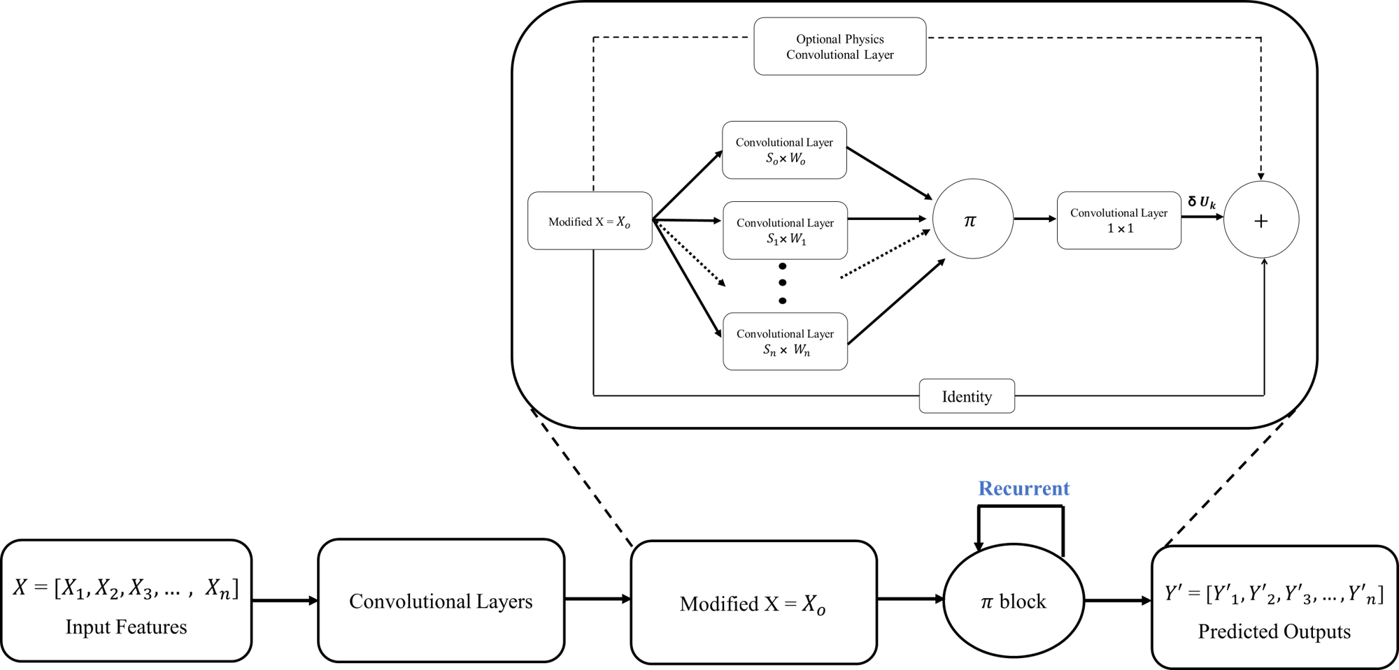
Figure 8: A schematic architecture for Physics-encoded Recurrent Convolutional Neural Network [40]. The architecture consists of X as initial inputs, convolutional layers, $X_{o}$ as full resolution initial state, unconventional convolutional block ($\pi$ block), and the predicted output layer Y’. Further, the $\pi$ block consists of multiple parallel convolutional layers whose operations are defined as $S_{n}\crossproduct W_{n}$, where n is the number of layers; $\pi$ carries out element-wise product and $+$ carries out element-wise addition.

The PeRCNN architecture was tested on two datasets representing 2D Burgers and 3D Gray-Scott reaction-diffusion equations [40]. In both cases, PeRCNN was compared with Convolutional LSTM [282], Deep Residual Network [283], and Deep Hidden Physics Models [176] in terms of accuracy (root-mean-squared-error, RMSE), data noise/scarcity, and generalization. The comparison for the 2D Burgers’ dataset is shown in Fig. 9(a), adapted from [40]. The accumulative RMSE for PeRCNN began with a larger value in the training region (due to 10 percent Gaussian noise in the data) and reduced as additional time steps were assessed. The accumulative RMSE for PeRCNN slightly increases in the extrapolation phase (as a measure of the model’s generalization), but clearly surpasses all other algorithms in terms of long-term extrapolation. Rao et al. [273] also used PeRCNN for discovering spatiotemporal PDEs from scarce and noisy data and demonstrated its effectiveness and superiority compared to baseline models.

Ren et al. [284] proposed a hybrid algorithm combining PeRCNN and PiNN to solve the limitations in low-dimensional spatiotemporal parameterization encountered by PgNNs and PiNNs. In the resultant physics-informed convolutional-recurrent network, dubbed as PhyCRNet, an encoder-decoder convolutional LSTM network is proposed for low-dimensional spatial feature extraction and temporal evolution learning. In PhyCRNet, the loss function is specified as aggregated discretized PDE residuals. The boundary conditions are hard-coded in the network via designated padding, and initial conditions are defined as the first input state variable for the network. Autoregressive and residual connections that explicitly simulate time marching were used to enhance the networks. This method ensures generalization to a variety of initial and boundary condition scenarios and yields a well-posed optimization problem in network training. Using PhyCRNet, it is also possible to simultaneously enforce known conservation laws into the network (e.g., mass conservation can be enforced by applying a stream function as the solution variable in the network for fluid dynamics) [284]. Ren et al. [284] evaluated and validated the performance of PhyCRNet using several non-linear PDEs compared to state-of-the-art baseline algorithms such as the PiNN and auto-regressive dense encoder-decoder model [269]. A comparison between PhyCRNet and PiNN to solve Burgers’ equation is shown in Fig. 9(b) [284]. Results obtained by Ren et al. [284] clearly demonstrated the superiority of the PhyCRNet methodology in terms of solution accuracy, extrapolability, and generalizability.

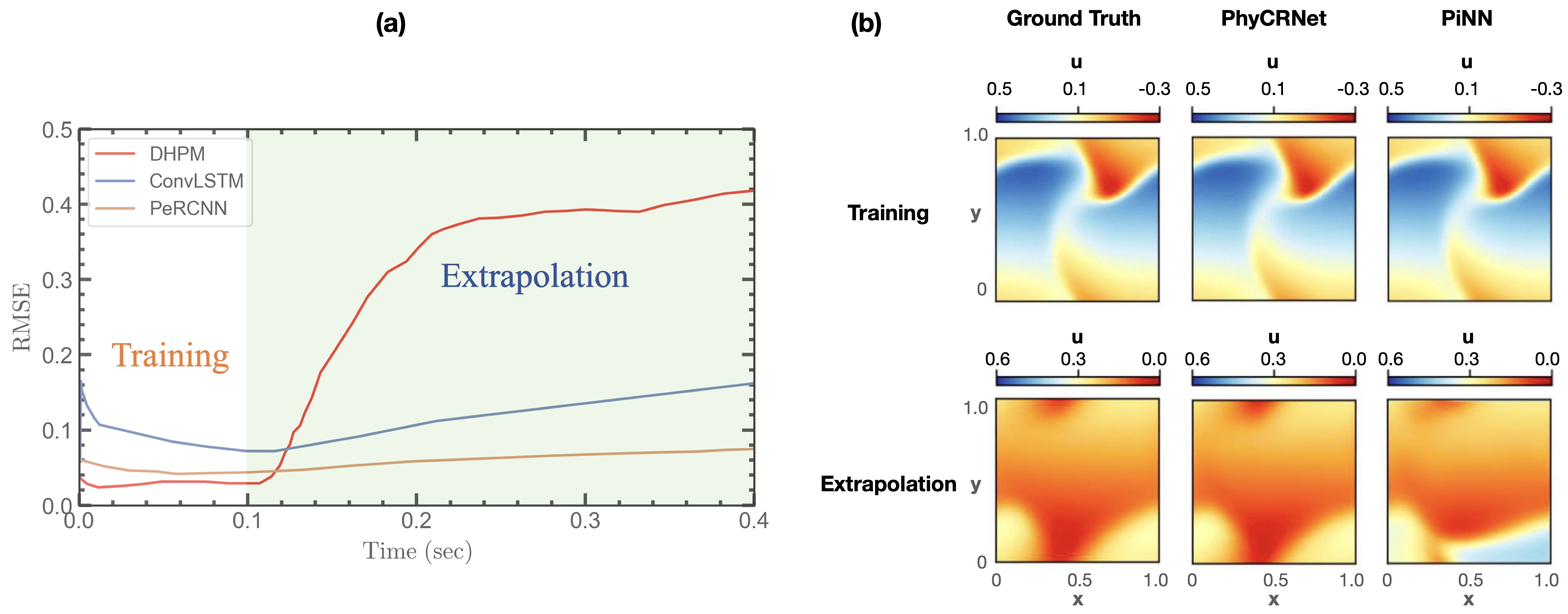
Figure 9: Panel (a) shows a comparison of error propagation in the training and extrapolation phases for a physics encoded recurrent convolutional neural network (PeRCNN), deep hidden physics model (DHPM), and a convolutional LSTM (ConvLSTM) modeling 2D Burgers’ dataset (adapted from Rao et al. [40]). Panel (b) shows a comparison between the predictions by PhyCRNet and PiNN for 2D Burgers’ equations. The predicted velocity field in x direction is compared at the training time of $t=1\leavevmode\nobreak\ s$, and at the extrapolation time of $t=3\leavevmode\nobreak\ s$ (adapted from Ren et al. [284]).

4.2 Neural Ordinary Differential Equations (NeuralODE)

The neural ordinary differential equations (NeuralODE) method is another family of PeNN models in which the hidden state of the neural network is transformed from a discrete sequence to a continuous non-linear function by parametrizing the hidden state derivative using a differentiable function [53]. The output of the network is then computed using a traditional differential equation solver. During training, the error is back-propagated through the network as well as through the ODE solver without access to its internal operations. This architecture is feasible due to the fact that numerical linear algebra is the common underlying infrastructure for both scientific computing and deep learning, which is bridged by automated differentiation (AD) [285]. Because differential equations and neural networks are both differentiable, standard optimization and error backpropagation techniques can be used to optimize the network’s weights during training. Instead of learning the non-linear transformation directly from the training data, the model in NeuralODE learns the structures of the non-linear transformation. Therefore, due to the fact that the neural network optimization equations are differentiable, the physical differential equations can be encoded directly into a layer as opposed to adding more layers (e.g., deeper networks). This results in a shallower network mimicking an infinitely deep model that can be inferred continuously at any desired accuracy at reduced memory and computational cost [286]).

These continuous-depth models offer features that are lacking in PiNN and PgNNs, such as (i) a reduced number of parameters for supervised learning, (ii) constant memory cost as a function of depth, and (iii) continuous time-series learning (i.e., training with datasets acquired at arbitrary time intervals), just to name a few [53]. However, the error backpropagation may cause technical difficulties while training such continuous-depth networks. Chen et al. [53] computed gradients using the adjoint sensitivity method [287] while considering the ODE solver as a black box. They demonstrated that this method uses minimal memory, can directly control numerical error, and, most importantly, scales linearly with the problem size.

Ma et al. [288] compared the performance of discrete and continuous adjoint sensitivity analysis. They indicated that forward-mode discrete local sensitivity analysis implemented via AD is more efficient than reverse-mode and continuous forward and/or adjoint sensitivity analysis for problems with approximately fewer than 100 parameters. However, in terms of scalability, they showed that the continuous adjoint method is more efficient than the discrete adjoint and forward methods.

Several computational libraries have been implemented to facilitate the practical application of NeuralODE. Poli et al. [289] implemented the TorchDyn library to train NeuralODE models and be as accessible as regular plug-and-play deep learning primitives. Innes et al. [8] and Rackauckas et al. [286] developed GPU-accelerated Zygote and DiffEqFlux libraries in the Julia coding ecosystem to bring differentiable programming and universal differential equation solver capabilities together. As an example, they encoded the ordinary differential equation of motion, as the transformation function, into a neural network to simulate the trebuchet’s inverse dynamics [8]. As shown in Fig. 10, the network with classical layers takes the target location and wind speed as input and estimates the weight and angle of the projectile to hit the target. These outputs are fed into the ODE solver to calculate the achieved distance. The model compares the predicted value with the target location and backpropagates the error through the entire chain to adjust the weights of the network. This PeNN model solves the trebuchet’s inverse dynamics on a personal computer 100x faster than a classical optimization algorithm for this inverse problem. Once trained, this network can be used to aim at any blind target, not just the ones it was trained on; hence, the model is both accelerated and predictive.

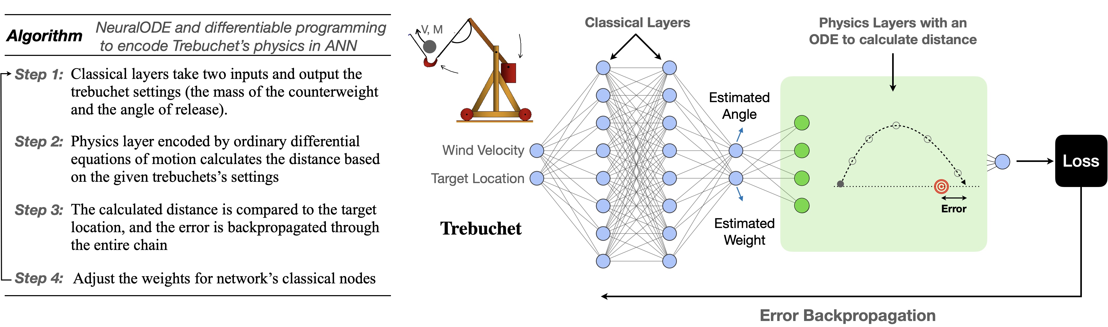
Figure 10: A NeuralODE architecture that leverages differentiable programming to model the inverse dynamics of a trebuchet. This simple network is 100x faster than direct optimization (adapted from Innes et al. [8]).

NeuralODE has also been integrated with PiNN models, dubbed as PiNODE, in order to further constrain the network with known governing physics during training. Such an architecture consists of a neural network whose hidden state is parameterized by an ODE with a loss function similar to the PiNN’s loss function (see Fig. 5). The loss function penalizes the algorithm based on data and the strong form of the governing ODEs and backpropagates the error through the application of the adjoint sensitivity methods [288], to update the learnable parameters in the architecture. PiNODE can be deployed to overcome high bias (due to the use of first principles in scientific modeling) and high variance (due to the use of pure data-driven models in scientific modeling) problems. In other words, using PiNODE, prior physics knowledge in terms of ODE is integrated where it is available, and function approximation (e.g., neural networks) is used where it is not available. Lai et al. [290] used PiNODE to model the governing equations in the field of structural dynamics (e.g., free vibration of a 4-degree-of-freedom dynamical system with cubic non-linearity). They showed that PiNODE provides an adaptable framework for structural health monitoring (e.g., damage detection) problems. Roehrl et al. [291] tested PiNODE using a forward model of an inverted pendulum on a cart and showed the approach can learn the non-conservative forces in a real-world physical system with substantial uncertainty.

The application of neural differential equation has also been extended to learn the dynamics of PDE-described systems. Dulny et al. [292] proposed NeuralPDE by combining the Method of Lines (which represents arbitrarily complex PDEs by a system of ODEs) and NeuralODE through the use of a multi-layer convolutional neural network. They tested NeuralPDE on several spatiotemporal datasets generated from the advection-diffusion equation, Burgers’ equation, wave propagation equation, climate modeling, etc. They found that NeuralPDE is competitive with other DL-based approaches, e.g., ResNet [293]. The NeuralPDE’s limitations are set by the limitations of the Method of Lines, e.g., it cannot be used to solve elliptical second-order PDEs. Table 9 reports a non-exhaustive list of leading studies that leveraged PeNN to model different scientific problems.

Table 8: A non-exhaustive list of recent studies that leveraged PeNN to model different scientific problems.

PeNN Structure	Objective	Reference
PeRCNN	Hard-encoding prior knowledge into a neural network to model non-linear systems	[40]
PhyCRNet	Leveraging the benefits of PeRCNN and PiNN into a single architecture	[284]
NeuralODE	Developing a continuous-depth network by parametrizing the hidden state derivative using a differentiable function	[53]
Zygote / DiffEqFlux	Providing libraries in the Julia coding ecosystem to facilitate the practical application of NeuralODE.	[8, 286]
PiNODE	Integrating PiNN and NeuralODE to provide an adaptable framework for structural health monitoring	[290]
NeuralPDE	Combining the Method of Lines and NeuralODE to learn the dynamics of PDE-described systems	[292]
LaNN	Capturing symmetries in physical problems such as relativistic particle and double pendulum	[276]
SRNNs	Capturing dynamics of hamiltonian systems such as three-body and spring-chain system from observed trajectories	[278]
DDEC	Enforcing exact physics and extracting structure-preserving surrogate models	[280]

4.3 PeNNs Limitations

Despite the advancement of numerous PeNN models and their success in modeling complex physical systems, these new architectures also face several challenges. The most important one is attributed to the training. PeNN-based models promote continuous learning using the development of continuous-depth networks, which makes PeNNs more difficult to train than PgNNs and PiNNs. Considering this, most of the limitations faced by PgNN and PiNN (e.g., convergence rate, stability, scalability, sample size- and problem-dependency) are also faced by PeNN. In addition, PeNNs usually have complex architectures, and their implementation is not as straightforward as PiNNs or PgNNs. In spite of PeNNs’ implementation complexity, their efficient algorithms in the finite-dimensional setting, their ability to provide transferable solutions, their robustness against data scarcity, and their generalizability compared to PgNN and PiNN make them have a great potential to significantly accelerate traditional scientific computing for applications in computational fluid and solid mechanics.

5 Neural Operators, NOs

Most of the scientific deep learning methods discussed so far, e.g., PgNNs, PiNNs, and PeNNs, are generally designed to map the solution of a physical phenomenon for a single instance (e.g., a certain spatiotemporal domain and boundary conditions to solve a PDE using PiNN), and thus, must re-trained or further trained (e.g., transfer learning [294]) to map the solution under a different instant. Another way to alleviate this problem is to use neural operators that learn nonlinear mappings between function spaces [39, 295, 296]. Neural operators, thus, form another simulation paradigm that learns the underlying linear and nonlinear continuous operators using advanced architecture. These models, similar to PgNNs, enforce the physics of the problem using labelled input-output dataset pairs but provide enhanced generalization, interpretability, continuous learning, and computational efficiency compared to PgNNs as well as PiNNs and PeNNs [180, 53, 43].

This new paradigm uses mesh-invariant, infinite-dimensional operators based on neural networks that do not require a prior understanding of PDEs. Neural operators merely work with data to learn the resolution-invariant solution to the problem of interest [43]. In other words, neural operators can be trained on one spatiotemporal resolution and successfully inferred on any other [296]. This resolution-invariant feature is achieved using the fact that a neural operator learns continuous functions rather than discretized vectors, by parameterizing the model in function spaces [43, 296]. Note that PgNNs and PiNNs, for example using MLP, may also guarantee a small generalization error, but that is only achieved by sufficiently large networks. One distinct feature of neural operators is their robustness for applications requiring real-time inference [57]. Three main neural operators have been proposed recently, namely (i) deep operator networks (DeepONets) [56], (ii) Fourier neural operator (FNO) [180], and (iii) graph neural operator (GNO) [296, 297]. A recent review by Goswami et al. [57] extensively compared these neural operators. In this section, we briefly review DeepONets and FNO as the two prominent neural operators to be applied in computational fluid and solid mechanics.

5.1 Deep Operator Networks (DeepONets)

Lu et al. [39] developed deep operator networks (DeepONets) based on the universal approximation theorem for operators [298] that can be used to learn operators accurately and efficiently with very small generalization errors. Lu et al. [56] proposed two architectures known as stacked and unstacked for DeepONet. The stacked DeepONet architecture is shown in Fig. 11(a), which consists of one trunk network and multiple stacked branch networks, $k=1,2...,p$. The stacked DeepONet is formed by selecting the trunk network as a one-layer network with width p and each branch network as a one-hidden-layer network with width n. To learn an operator $G$:$s\rightarrow G(s)$, the stacked DeepONet architecture takes function $s$ as the input to branch networks and y (i.e., points in the domain of $G(s)$) as the input to the trunk network. Here, the vector $[(x_{1}),(x_{2}),...,(x_{m})]$ represents the finite locations of data, alternatively dubbed as sensors. The trunk network outputs $[t_{1},t_{2},...,t_{p}]^{T}\in\mathbb{R}^{p}$, and each branch network outputs a scalar represented by $b_{k}\in\mathbb{R}$, where $k=1,2...,p$. Next, the outputs generated by trunk and branch networks are integrated together as $G(s)(y)\approx\sum_{k=1}^{p}b_{k}(s(x_{1}),s(x_{2}),...s(x_{m}))t_{k}(y)$. The unstacked DeepONet architecture is also shown in Fig. 11(a), which consists of only one branch network (depicted in dark blue) and one trunk network. The unstacked DeepONet may be considered as a stacked DeepONet, in which all of the branch networks share the same set of parameters [56]. DeepONet was first used to learn several explicit operators, including integral and fractional Laplacians, along with implicit operators that represented deterministic and stochastic differential equations Lu et al. [56]. The two main advantages of DeepONets discussed by Lu et al. [56] are (i) small generalization error and (ii) rapid convergence of training and testing errors with respect to the quantity of the training data.

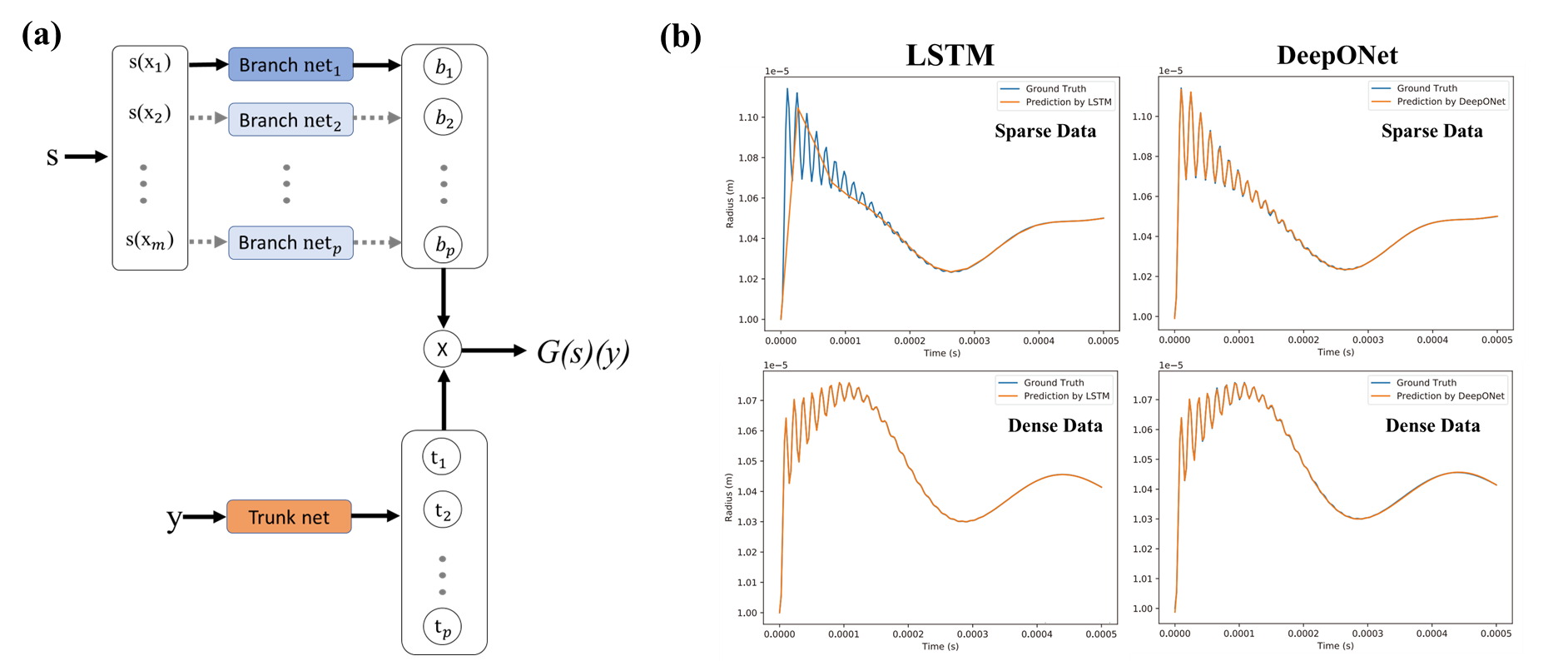
Figure 11: DeepONet for computational mechanics. Panel(a) depicts the general architecture of stacked DeepONets to learn an operator $G$:$s\rightarrow G(s)$. The stacked DeepONet reduces to an unstacked DeepONet when only one branch network (e.g., the one shown in dark blue) is used. Alternatively, the unstacked DeepONet may be considered as a stacked DeepONet, in which all of the branch networks share the same set of parameters [56]. Panel(b) shows a comparison between DeepONet and LSTM (i.e., PgNN) to model sparse and dense datasets representing the formation of a single bubble in response to time-varying changes in the ambient liquid pressure (adapted from Lin et al. [299]).

Lin et al. [299] showed the effectiveness of DeepONet against data density and placement, which is advantageous when no prior knowledge is available on how much training data is required or when there are strict limits on data acquisition (e.g., location accessibility). To this end, they employed DeepONet and LSTM (i.e., PgNN) to model datasets representing the formation of a single bubble in response to time-varying changes in the ambient liquid pressure. To generate datasets, they used Rayleigh–Plesset (R–P) as a macroscopic model and dissipative particle dynamics (DPD) as a microscopic model. They used Gaussian random fields to generate different pressure fields, which serve as input signals for this dynamical system. The results of the comparison are shown in Fig. 11(b). The top row shows the prediction results for the liquid pressure trajectory when only 20 data points are known per trajectory, i.e., sparse training data, and the bottom row shows the same but when 200 data points are known per trajectory, i.e., dense training data. As shown, regardless of how sparse the training data was, DeepONet was able to outperform LSTM to predict the liquid pressure trajectory.

In addition, they examined a case where the input was not contained inside the training input range, i.e., when the correlation length of the pressure field was outside of the training range. In this case, they were initially unable to make accurate predictions, but mitigated the issue by transferring learning to a pre-trained DeepONet trunk network and fine-tuning it with only a few additional data points. They also demonstrated that DeepONet can learn the mean component of the noisy raw data for the microscopic model without any additional data processing and that the computational time can be reduced from 48 CPU hours to a fraction of a second. These results confirmed that the DeepONet model can be applied across macroscopic and microscopic regimes of bubble growth dynamics, establishing the foundation for a unified neural network model that can seamlessly predict physics interacting across scales.

Oommen et al. [300] combined convolutional autoencoder architecture with DeepONet (CA-DeepONet) to learn the dynamic development of a two-phase mixture and speed up the time-to-solution for microstructure evolution prediction. In low-dimensional latent space, the convolutional autoencoder was utilized to provide a compact representation of microstructure data, while DeepONet was employed to learn mesoscale dynamics of microstructure evolution from the autoencoder’s latent space. Then, the decoder component of the convolutional autoencoder reconstructs the evolution of the microstructure based on DeepONet’s predictions. The trained DeepOnet architecture can then be used to speed up the numerical solver in extrapolation tasks or substitute the high-fidelity phase-field numerical solver in interpolation problems.

By taking inspiration from PiNNs for sparse data domains, DeepONets can also be trained with very sparse labeled datasets while incorporating known differential equations into the loss function. This approach results in Physics-informed DeepONets (Pi-DeepONets) [301, 302]. Wang et al. [301] employed Pi-DeepONets for benchmark problems such as diffusion reaction, Burger’s equation, advection equation, and eikonal equation. In comparison to vanilla DeepONet, the result reveals significant improvements in predictive accuracy, generalization performance, and data efficiency. Furthermore, Pi-DeepONets can learn a solution operator without any paired input-output training data, allowing them to simulate nonlinear and non-equilibrium processes in computational mechanics up to three orders of magnitude quicker than traditional solvers [301].

Goswami et al. [302] used a physics-informed variational formulation of DeepONet (Pi-V-DeepONet) for brittle fracture mechanics. The training of the Pi-V-DeepONet was conducted using the governing equations in a variational form and some labeled data. They used the Pi-V-DeepONet framework to determine failure pathways, failure zones, and damage along failure in brittle fractures for quasi-brittle materials. They trained the model to map the initial configuration of a defect (e.g., crack) to the relevant fields of interest (e.g., damage and displacements, see Fig. 12). They showed that their model can rapidly predict the solution to any initial crack configuration and loading steps. In brittle fracture mechanics, the proposed model can be employed to enhance the design, evaluate reliability, and quantify uncertainty.

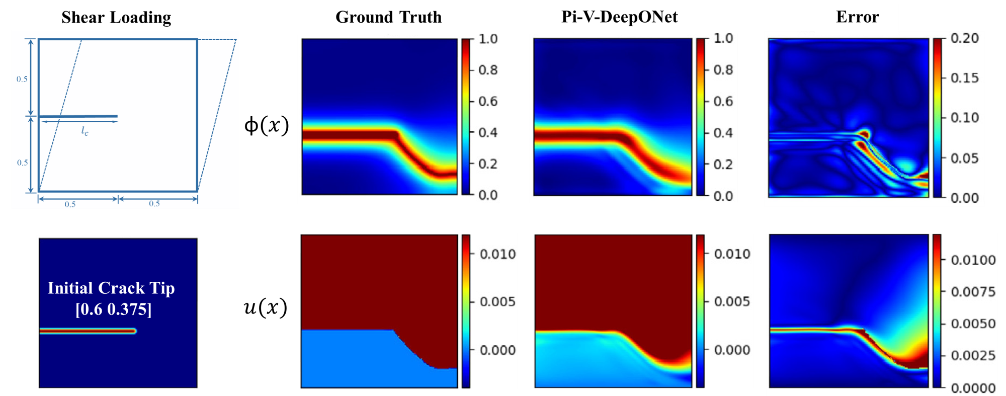
Figure 12: A comparison between Pi-V-DeepONet and isogeometric FEM analysis to predict the final damage path for the shear failure of a single-edge notched plate. The initial geometry of the single-edge notched plate, shear loading, and the initial configuration of the crack are shown on the left panels. The right panels show the comparisons for the phase field, $\phi(x)$, and displacement along the x-axis, $u(x)$, as well as the corresponding error between the prediction and ground truth (adapted from Goswami et al. [302]).

Due to the high cost of evaluating integral operators, DeepONets may face difficulty to develop effective numerical algorithms capable of replacing convolutional or recurrent neural networks in an infinite-dimensional context. Li et al. [180] made an effort along this line and developed an operator regression by parameterizing the integral kernel in the Fourier space and termed it the Fourier neural operator (FNO). In the next section, we discuss the core architecture of FNO and the recent developments around it.

5.2 Fourier Neural Operator (FNO)

In order to benefit from neural operators in infinite-dimensional spaces, Li et al. [180] developed a neural operator in the Fourier space, dubbed as FNO, with a core architecture schematically shown in Fig. 13. The training starts with an input $X$, which is subsequently elevated to a higher dimensional space by a neural network $S$. The second phase entails the use of several Fourier layers of integral operators and activation functions. In each Fourier layer, the input is transformed using (i) a Fourier transform, $F$; (ii) a linear transform, $T$, on the lower Fourier modes that filters out the higher modes; and (iii) an inverse Fourier transform, $F^{-1}$. The input is also transformed using a local linear transform, $W$, before the application of the activation function, $\sigma$. The Fourier layers are designed to be discretization-invariant due to the fact that they learn from functions that are discretized arbitrarily. Indeed, the integral operator is applied in convolution and is represented as a linear transformation in the Fourier domain, allowing the FNO to learn the mapping over infinite-dimensional spaces. The result of the Fourier layer is projected back to the target dimension in the third phase using another neural network $M$, which eventually outputs the desired output $Y^{\prime}$ [180]. Unlike other DL methods, the FNO model’s error is consistent regardless of the input and output resolutions (e.g., in PgNN methods, the error grows with the resolution).

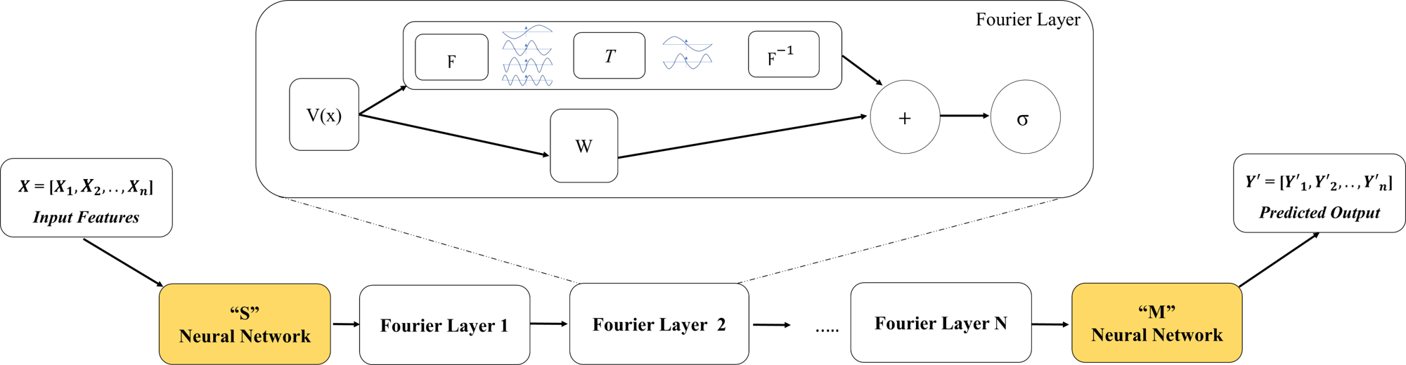
Figure 13: A schematic architecture of the Fourier Neural Operator (FNO) [180]. Here, X is the inputs, S and M are the neural network for dimensional space operation, and Y’ is the predicted outputs. Each of the Fourier layers consists of v(x) as the initial state, $\mathcal{F}$ layer that performs Fourier transform, $T$ layer that performs linear transform, $\mathcal{F}^{-1}$ layer that performs inverse Fourier transform, W layer for local linear transform, + block that carries out element-wise addition on W, and the final output from the $\mathcal{F}^{-1}$ layer. The final product from element-wise addition is passed on to a $\sigma$ layer.

Li et al. [180] employed FNO on three different test cases, including the 1D Burgers’ equation, the 2D Darcy flow equation, and the 2D Navier-Stokes equations. For each test case, FNO was compared with state-of-the-art models. In particular, for Burgers’ and Darcy’s test cases, the methods used for comparison were the conventional ANN (i.e., PgNN), reduced bias method [303], fully convolutional networks [304], principal component analysis as an encoder in the neural network [295], graph neural operator [296], and low-rank decomposition neural operator (i.e., unstacked DeepONet [39]). In all test cases, FNO yielded the lowest relative error. The models’ error comparisons for 1D Burgers’ and 2D Darcy flow equations are depicted in Fig. 14, adapted from [180].

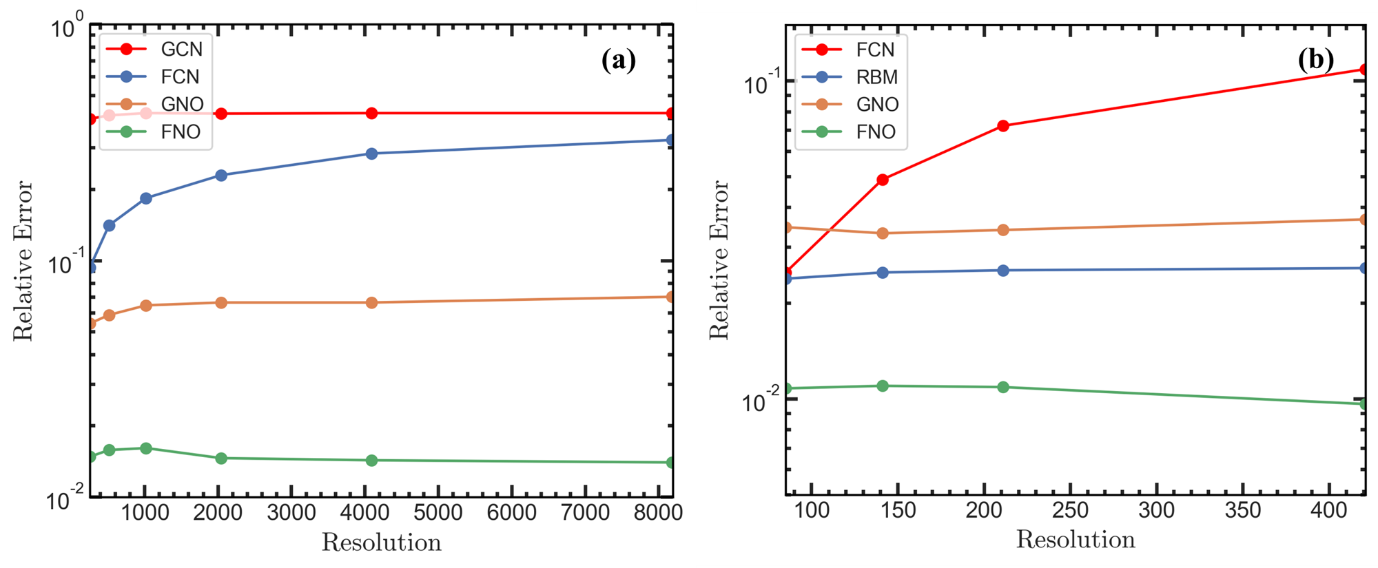
Figure 14: Error comparison between FNO and other state-of-the-art methods (reduced bias method (RBM), fully convolutional network (FCN), graph neural operator (GNO), and graph convolutional network (GCN)) for (a) Burgers’ equation and (b) Darcy’s Flow equation at different resolutions (adapted from Li et al. [180]).

The FNO model, as stated, can be trained on a specific resolution and tested on a different resolution. Li et al. [180] demonstrated this claim by training a FNO on the Navier-Stokes equations for a 2D test case with a resolution of 64$\times$64$\times$20 ($n_{x},n_{y},n_{t}$) standing for spatial (x, y) and time resolution, and then evaluating it with a resolution of 256$\times$256$\times$80, as shown in Fig. 15(a). In comparison to other models, the FNO was the only technique capable of performing resolution downscaling both spatially and temporally [180]. FNOs can also achieve several orders of magnitude speedup factors over conventional numerical PDE solvers. However, they have only been used for 2D or small 3D problems due to the large dimensionality of their input data, which increases the number of network weights significantly. With this problem in mind, Grady et al. [305] proposed a parallelized version of FNO based on domain-decomposition to resolve this limitation. Using this extension, they were able to use FNO in large-scale modeling, e.g., simulating the transient evolution of the CO2 plume in subsurface heterogeneous reservoirs as a part of the carbon capture and storage (CCS) technology [306], see Fig. 15(b). The input to the network (with a similar architecture to the one proposed by Li et al. [180]) was designed to be a tensor containing both the permeability and topography fields at each 3D spatial position using a 60$\times$60 $\times$64 ($n_{x},n_{y},n_{z}$) resolution and the output was 60$\times$60$\times$64$\times n_{t}$. For a time resolution of $n_{t}=30\leavevmode\nobreak\ s$, they found that the parallelized FNO model was 271 times faster (without even leveraging GPU) than the conventional porous media solver while achieving comparable accuracy. Wen et al. [307] also proposed U-FNO, an extension of FNO, to simulate multiphase flows in porous media, specifically CO2-water multiphase flow through a heterogeneous medium with broad ranges of reservoir conditions, injection configurations, flow rates, and multiphase flow properties. They compared U-FNO with FNO and CNN (i.e., PgNN) and showed that the U-FNO architecture provides the best performance for both gas saturation and pressure buildup predictions in highly heterogeneous geological formations. They also showed that the U-FNO architecture enhances the training accuracy of the original FNO, but does not naturally enable the flexibility of training and testing at multiple discretizations.

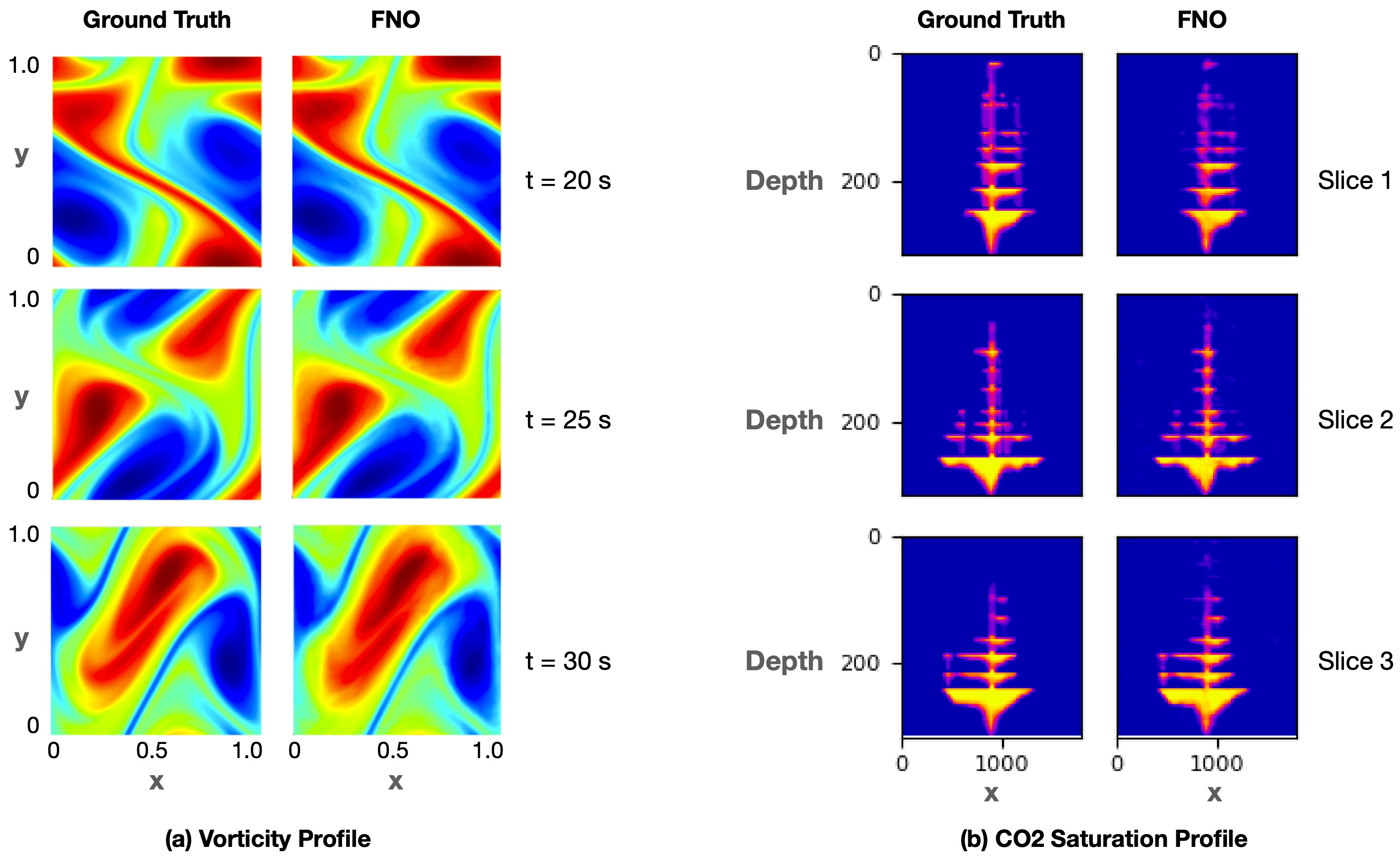
Figure 15: A qualitative comparison between predictions made by the Fourier neural operator (FNO) and ground truth values. Panel (a) shows the comparison for a FNO model trained on 64$\times$64$\times$20 resolution ($n_{x},n_{y},n_{t}$) and evaluated on 256$\times$256$\times$80 resolution to solve 2D Navier-Stokes equations (adapted from Li et al. [180]). Panel (b) shows the comparison for a parallelized FNO model trained to solve large-scale 3D subsurface CO2 flow modeling evaluated at 60$\times$60$\times$64$\times n_{t}$ resolution (adapted from Grady et al. [305]).

You et al. [308] proposed an implicit Fourier neural operator (IFNO) to model the complex responses of materials due to their heterogeneity and defects without using conventional constitutive models. The IFNO model captures the long-range dependencies in the feature space, and as the network becomes deeper, it becomes a fixed-point equation that yields an implicit neural operator (e.g., it can mimic displacement/damage fields). You et al. [308] demonstrated the performance of IFNO using a series of test cases such as hyperelastic, anisotropic, and brittle materials. Fig. 16 depicts a comparison between IFNO and FNO for the transient propagation of a glass-ceramic crack [308]. As demonstrated, IFNO outperforms FNO (in terms of accuracy) and conventional constitutive models (in terms of computational cost) to predict the displacement field.

The FNO model has also been hybridized with PiNN to create the so-called physics-informed neural operator (PiNO) [43]. The PiNO framework is a combination of operating-learning (i.e., FNO) and function-optimization (i.e., PiNN) frameworks that improves convergence rates and accuracy over both PiNN and FNO models. This integration was suggested to address the challenges in PiNN (e.g., generalization and optimization, especially for multiscale dynamical systems) and the challenges in FNO (e.g., the need for expensive and impractical large training datasets) [43]. Li et al. [43] deployed the PiNO model on several benchmark problems (e.g., Kolmogorov flow, lid-cavity flow, etc.) to show that PiNO can outperform PiNN and FNO models while maintaining the FNO’s exceptional speed-up factor over other solvers.

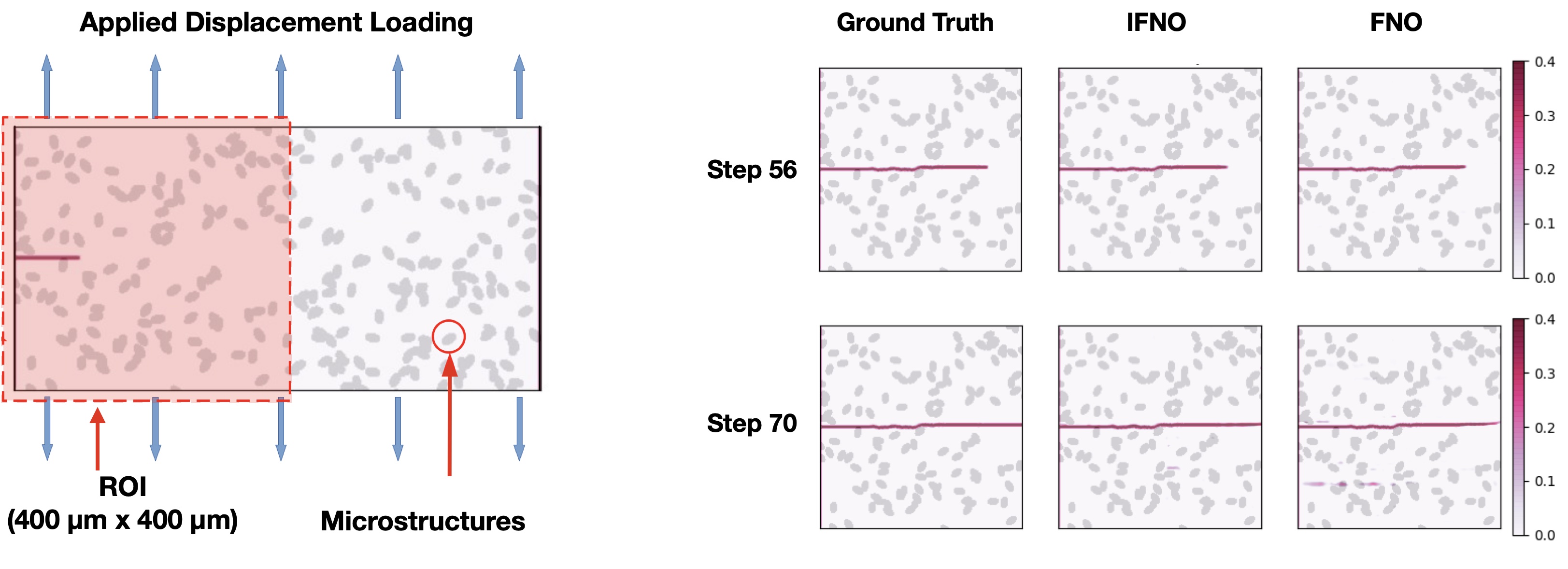
Figure 16: A comparison between the implicit Fourier neural operator (IFNO) and FNO models to predict crack propagation and damage field within a region of interest (ROI) in a pre-cracked glass-ceramics experiment with randomly distributed material property fields (adapted from You et al. [308]).

Table 9: A non-exhaustive list of recent studies that leveraged Neural Operators to model different scientific problems.

NO Structure	Objective	Reference
DeepONets	Learning non-linear operators accurately and efficiently with low generalization error	[56]
CADeepONet	Learning dynamic development of a two-phase mixture and reducing solution time for predicting microstructure evolution	[300]
Pi-DeepONets	Integrating DeepONets and PiNN to relax the requirement for a large training dataset while improving generalization and predictive accuracy	[301]
V-DeepONet	Generating a fast and generalizable surrogate model for brittle fracture mechanics	[302]
FNO	Providing a mesh- and discretization-invariant model to be inferred at any arbitrary spatiotemporal resolutions	[180]
Parallelized FNO	Extending FNO based on domain-decomposition to model large-scale three-dimensional problems	[305]
U-FNO	Enhancing the training and testing accuracy of FNO for large-scale, highly heterogeneous geological formations	[307]
IFNO	capturing the long-range dependencies in the feature space that yields an implicit neural operator to model the complex responses of materials due to their heterogeneity and defects	[308]
PINO	Integrating PiNN and FNO to relax the requirement for a large training dataset while enhancing generalization and optimization	[43]

5.3 NOs Limitations

DeepONet [39] and FNO [180], as the two most common neural operators to date, share some commonalities while also having significant differences. The DeepONet architecture was inspired by Chen and Chen [298]’s universal approximation theorems, whereas the FNO was architecture established on parameterizing the integral kernel in Fourier space. However, FNO in its continuous form can be viewed as DeepONet with a specific architecture of the trunk (expressed by a trigonometric basis) and branch networks [309]. FNO, unlike DeepONet, discretizes both the input function and output function via point-wise evaluations in an equally spaced mesh. Therefore, after network training, FNO can only predict the solution in the same mesh as the input function, but DeepONet can make predictions at any arbitrary location. FNO also requires a full field of observation data for training, whereas DeepONet is more flexible, with the exception of POD-DeepONet [310], which requires a full field of observation data to calculate the proper orthogonal decomposition (POD) modes [310]. DeepONet, FNO, and their various variants still face some limitations, especially when applied to large multi-physics problems, that necessitate further investigations.

• Neural operators are purely data-driven and require relatively large training datasets, therefore they face constraints when applied to problems where data acquisition is complex and/or costly [310]. Integration with PiNN can resolve this issue to some extent for problems where the underlying physics is fully known and can be integrated into the loss function [301]. Also, for practical applications, training the NOs just based on the governing equations in the loss function may produce inaccurate predictions; instead, a hybrid physics-data training is recommended [301].

• DeepONet and FNO are typically limited to basic geometry and/or structured data (e.g., 2D or small 3D problems) due to the large dimensionality of their input data that increases the number of network weights significantly) [310]. They are also prone to over-fitting as the number of trainable parameters increases, making the training process more difficult [311]. IFNOs have addressed this challenge to some extent [308]. In IFNO, the solution operator is first formulated as an implicitly defined mapping and then modeled as a fixed point. The latter aims to overcome the challenge of network training in the case of deep layers, and the former minimizes the number of trainable parameters and memory costs. Nonetheless, due to the finite size of the neural network architecture, the convergence of NOs (e.g., DeepONet) error with respect to the size of the training data becomes algebraic for large datasets; it is desired to be exponential [310].

• FNO might not be reliable for discontinuous functions as it relies on the Fourier transformation. This is mitigated to some extent by DeepONet, as it was shown to perform well for functions with discontinuity (e.g., compressible Euler equations) [310].

Despite these limitations, neural operators are the leading algorithms in a variety of real-time inference applications, including autonomous systems, surrogates in design problems, and uncertainty quantification [57].

6 Conclusions and Future Research Directions

A considerable number of research topics collectively support the efficacy of combining scientific computing and deep learning approaches. In particular, this combination improves the efficiency of both forward and inverse modeling for high-dimensional problems that are prohibitively expensive, contain noisy data, require a complex mesh, and are governed by non-linear, ill-posed differential equations. The ever-increasing computer power will continue to further furnish this combination by allowing the use of deeper neural networks and considering higher-dimensional interdependencies and design space.

Table 10: A comparison of the main characteristics of PgNNs, PiNNs, PeNNs, and NOs to model non-linear multiscale phenomena in computational fluid and solid mechanics.

Feature	PgNNs	PiNNs	PeNNs	NOs
Accelerating Capability	✓	✓	✓	✓
Mesh-free Simulation	✓	✓	✓	✓
Straightforward Network Training	✓	✗	✗	✗
Training without Labeled Data	✗	✓	✗	✗
Physics-informed Loss Function	✗	✓	✓	✓
Continuous Solution	✗	✓	✓	✓
Spatiotemporal Interpolation	✗	✓	✓	✓
Physics Encoding	✗	✗	✓	✗
Efficient Operator Learning	✗	✗	✗	✓
Continuous-depth Models	✗	✗	✓	✗
Spatiotemporal Extrapolation	✗	✗	✓	✓
Solution Transferability	✗	✗	✓	✓
Efficient Real-time Predictions	✗	✗	✗	✓

The combination of scientific computing and deep learning approaches also surpasses traditional computational mechanics solvers in a number of prevalent scenarios in practical engineering. For example, a sparse dataset obtained experimentally for a complex (i.e., hard-to-acquire data) phenomenon cannot be simply integrated with traditional solvers. Whereas using DL, the following tasks can be performed: (i) PgNN-based models can be applied to the sparse data to extract latent interdependencies and conduct spatiotemporal downscaling or upscaling (i.e., interpolated data); (ii) PiNN-based models can be applied to the interpolated data to deduce governing equations and potentially unknown boundary or initial conditions of the phenomena (i.e., strong mathematical form); (iii) PeNN-based models can be used to combine the interpolated data and the strong mathematical form to conduct extrapolation exploration; and (iv) NO-based models can be applied to make real-time predictions of the complex dynamics. Therefore, the combination of DL-based methods and traditional scientific computing methods provides scientists with a cost-effective toolbox to explore problems across different scales that were deemed far-fetched computationally. To this end, several other breakthroughs in DL are required to enable the use of PgNNs, PiNNs, PeNNs, and NOs in large-scale three-dimensional (or multi-dimensional) problems. For instance, the training of complex DL models (e.g., PiNNs, PeNNs, and NOs) should be accelerated using different parallelization paradigms.

Table 10 compares the main characteristics of the PgNNs, PiNNs, PeNNs, and NOs. The PgNN-based models suffer mainly from their statistical training process, for which they require large datasets. They map carefully curated training datasets only based on correlations in statistical variations, and hence, their predictions are naturally physics-agnostic. The PiNN-based models suffer mainly from the presence of competing loss terms that may destabilize the training process. PiNN is also a solution learning algorithm with limited generalizability due to its inability to learn the physical operation of a specific phenomenon. Models based on PeNNs and NOs, on the other hand, may experience low convergence rates and require a large volume of paired, structured datasets, leading to highly expensive training.

Considering the effectiveness of this new challenge of combining scientific computing and DL, future studies can be divided into three distinct categories: (i) Improving algorithms: Developing advanced variants of PgNNs, PiNNs, PeNNs and NOs that offer simpler implementation with enhanced convergence rate; faster training in multi-dimensional and multi-physics problems; higher accuracy and generalization to unseen conditions while using sparse training datasets, more robust to be used in real time forecasting; better adaptability to multi-spatiotemporal-resolutions, more flexibility to encode various types of governing equations (e.g., all PDE types, closure laws, data-driven laws, etc.), and provide a closer tie with a plethora of traditional solvers; (ii) Considering causalities: Developing a causal training algorithm (e.g., causal Q-learning [312]) that restores physical causality during the training of PgNN, PiNN, and PeNN models by re-weighting the governing equations (e.g., PDEs) residual loss at each iteration. This line of research will allow for the development of causality-conforming variants of PgNN, PiNN, and PeNN algorithms that can bring new opportunities for the application of these algorithms to a wider variety of complex scenarios across diverse domains; (iii) Expanding applications: Leveraging the potentials of PgNNs, PiNNs, PeNNs, and NOs in problems with complex anisotropic materials (e.g., flow in highly heterogeneous porous media, metal and non-metal particulate composites, etc.); problems with multiscale multi-physics phenomena (e.g., magnetorheological fluids, particle-laden fluids, dry powder dynamics, reactive transport, unsaturated soil dynamics, etc.); problems with multi-resolution objectives and extensive spatiotemporal downscaling or upscaling (e.g., global and regional climate modeling, geosystem reservoir modeling, etc.); and structural health monitoring (e.g., crack identification and propagation, hydrogen pipeline leakage, CO2 plume detection, etc.); and (iv) Coupling solvers: Coupling PgNNs, PiNNs, and PeNNs as well as NOs with open-source computational mechanics packages such as OpenIFEM, OpenFOAM, Palabos, LAMMPS, LIGGGHTS, MOOSE, etc. This line of research will allow for faster surrogate modeling and, hence, faster development of next-generation solvers. It also expedites community and industry adoption of the combined scientific-DL computational paradigm.

7 Acknowledgements

S.A.F. would like to acknowledge supports from the Department of Energy Biological and Environmental Research (BER) (award no. DE-SC0023044), National Science Foundation Partnership for Research and Education in Materials (PREM) (award no. DMR-2122041), and Texas State University Multidisciplinary Internal Research Grant (MIRG) (award no. 9000003028).

C.F. would like to acknowledge supports from FEDER funds through the COMPETE 2020 Programme and National Funds through FCT (Portuguese Foundation for Science and Technology) under the projects UID-B/05256/2020, UID-P/05256/2020 and MIT-EXPL/TDI/0038/2019-APROVA-Deep learning for particle-laden viscoelastic flow modelling (POCI-01-0145-FEDER-016665) under the MIT Portugal program.

8 Conflict of Interest

The authors declare no conflict of interest.

References

- Vinuesa and Brunton [2022] Ricardo Vinuesa and Steven L Brunton. Enhancing computational fluid dynamics with machine learning. Nature Computational Science, 2(6):358–366, 2022. DOI: https://doi.org/10.1038/s43588-022-00264-7.
- Mianroodi et al. [2021] J. R. Mianroodi, N. H. Siboni, and D. Raabe. Teaching solid mechanics to artificial intelligence - a fast solver for heterogeneous materials. NPJ Computational Materials, 7:99, 2021. DOI: https://doi.org/10.1038/s41524-021-00571-z.
- Kim et al. [2021] Y. Kim, C. Yang, K. Park, G. X. Gu, and R. Seunghwa. Deep learning framework for material design space exploration using active transfer learning and data augmentation. npj Computational Materials, 7:140, 2021. DOI: https://doi.org/10.1038/s41524-021-00609-2.
- Dino et al. [2020] H. I. Dino, S. R. Zeebaree, A. A. Salih, R. R. Zebari, Z. S. Ageed, H. M. Shukur, L. M. Haji, and S. S. Hasan. Impact of process execution and physical memory-spaces on os performance. Technology Reports of Kansai University, 62(5):2391–2401, 2020.
- Im et al. [2021] S. Im, J. Lee, and M. Cho. Surrogate modeling of elasto-plastic problems via long short-term memory neural networks and proper orthogonal decomposition. Computer Methods in Applied Mechanics and Engineering, 385:114030, 2021. DOI: https://doi.org/10.1016/j.cma.2021.114030.
- Karniadakis et al. [2021] G. E. Karniadakis, I. G. Kevrekidis, L. Lu, P. Perdikaris, S. Wang, and L. Yang. Physics-informed machine learning. Nature Reviews Physics, 3(6):422–440, 2021. DOI: https://doi.org/10.1038/s42254-021-00314-5.
- Arman and Anthony [2022] S. Arman and W. Anthony. Physics-inspired architecture for neural network modeling of forces and torques in particle-laden flows. Computers and Fluids, 238:105379, 2022. DOI: https://doi.org/10.1016/j.compfluid.2022.105379.
- Innes et al. [2019] M. Innes, A. Edelman, K. Fischer, C. Rackauckas, E. Saba, V.B. Shah, and W. Tebbutt. A differentiable programming system to bridge machine learning and scientific computing. arXiv preprint arXiv:1907.07587, 2019. DOI: https://doi.org/10.48550/arXiv.1907.07587.
- Brunton et al. [2020] S. L. Brunton, B. R. Noack, and P. Koumoutsakos. Machine learning for fluid mechanics. Annual Review of Fluid Mechanics, 52:477–508, 2020. DOI: https://doi.org/10.1146/annurev-fluid-010719-060214.
- Cai et al. [2022a] S. Cai, Z. Mao, Z. Wang, M. Yin, and G. E. Karniadakis. Physics-informed neural networks (pinns) for fluid mechanics: A review. Acta Mechanica Sinica, pages 1–12, 2022a. DOI: https://doi.org/10.1007/s10409-021-01148-1.
- Kutz [2017] J. N. Kutz. Deep learning in fluid dynamics. Journal of Fluid Mechanics, 814:1–4, 2017. DOI: https://doi.org/10.1017/jfm.2016.803.
- Shi et al. [2019] Z. Shi, E. Tsymbalov, M. Dao, S. Suresh, A. Shapeev, and J. Li. Deep elastic strain engineering of bandgap through machine learning. Proc. Natl. Acad. Sci., 116:4117–4122, 2019. DOI: https://doi.org/10.1073/pnas.1818555116.
- Haghighat et al. [2021a] E. Haghighat, M. Raissi, A. Moure, H. Gomez, and R. Juanes. A physics-informed deep learning framework for inversion and surrogate modeling in solid mechanics. Computer Methods in Applied Mechanics and Engineering, 379:113741, 2021a. DOI: https://doi.org/10.1016/j.cma.2021.113741.
- Pilania et al. [2013] G. Pilania, C. Wang, Jiang X., S. Rajasekaran, and R. Ramprasad. Accelerating materials property predictions using machine learning. Sci. Rep., 3:1–6, 2013. DOI: https://doi.org/10.1038/srep02810.
- Butler et al. [2018] K. T. Butler, D. W. Davies, H. Cartwright, O. Isayev, and A. Walsh. Machine learning for molecular and materials science. Nature, 559:547–555, 2018. DOI: https://doi.org/10.1038/s41586-018-0337-2.
- Brunton and Kutz [2019] S. L. Brunton and J. N. Kutz. Methods for data-driven multiscale model discovery for materials. J. Phys. Mater., 2:044002, 2019. DOI: https://doi.org/10.1088/2515-7639/ab291e.
- Bedolla et al. [2020] E. Bedolla, L. C. Padierna, and R. Castaneda-Priego. Machine learning for condensed matter physics. Journal of Physics: Condensed Matter, 33(5):053001, 2020. DOI: https://doi.org/10.1088/1361-648X/abb895.
- Kochkov et al. [2021] D. Kochkov, J. A. Smith, A. Alieva, Q. Wang, M. P. Brenner, and S. Hoyer. Machine learning–accelerated computational fluid dynamics. Proceedings of the National Academy of Sciences, 118:e2101784118, 2021. DOI: https://doi.org/10.1073/pnas.2101784118.
- Tran et al. [2017] D. Tran, M. D. Hoffman, R. A. Saurous, E. Brevdo, K. Murphy, and D.M. Blei. Deep probabilistic programming. arXiv preprint arXiv:1701.03757, 2017. DOI: https://doi.org/10.48550/arXiv.1701.03757.
- Jin et al. [2017] K. H. Jin, M.T. McCann, E. Froustey, and M. Unser. Deep convolutional neural network for inverse problems in imaging. IEEE Transactions on Image Processing, 26(9):4509–4522, 2017. DOI: https://doi.org/10.1109/TIP.2017.2713099.
- Lai et al. [2022] Z. Lai, Q. Chen, and L. Huang. Machine-learning-enabled discrete element method: Contact detection and resolution of irregular-shaped particles. International Journal for Numerical and Analytical Methods in Geomechanics, 46(1):113–140, 2022. DOI: https://doi.org/10.1002/nag.3293.
- Faroughi et al. [2022a] S. A. Faroughi, A. I. Roriz, and C. Fernandes. A meta-model to predict the drag coefficient of a particle translating in viscoelastic fluids: a machine learning approach. Polymers, 14(3):430, 2022a. DOI: https://doi.org/10.3390/polym14030430.
- Taylor [1715] B. Taylor. Methodus incrementorum directa & inversa. Auctore Brook Taylor, LL. D. & Regiae Societatis Secretario. typis Pearsonianis: prostant apud Gul. Innys ad Insignia Principis in …, 1715.
- Alder and Wainwright [1957] B. J. Alder and T. E. Wainwright. Phase transition for a hard sphere system. The Journal of chemical physics, 27(5):1208–1209, 1957.
- Clough [1960] R. W. Clough. The finite element method in plane stress analysis. In Proceedings of 2nd ASCE Conference on Electronic Computation, Pittsburgh Pa., Sept. 8 and 9, 1960, 1960.
- Smagorinsky [1963] J. Smagorinsky. General circulation experiments with the primitive equations: I. the basic experiment. Monthly weather review, 91(3):99–164, 1963.
- Cundall and Strack [1979] P. A. Cundall and O. Strack. A discrete numerical model for granular assemblies. Géotechnique, 29:47–65, 1979. DOI: https://doi.org/10.1680/geot.1979.29.1.47.
- McDonald [1971] P. W. McDonald. The computation of transonic flow through two-dimensional gas turbine cascades, volume 79825. American Society of Mechanical Engineers, 1971.
- Peskin [1972] C. S. Peskin. Flow patterns around heart valves: a numerical method. Journal of computational physics, 10(2):252–271, 1972.
- Lucy [1977] L. B. Lucy. A numerical approach to the testing of the fission hypothesis. The astronomical journal, 82:1013–1024, 1977.
- D’Humieres et al. [1986] D. D’Humieres, P. Lallemand, and U. Frisch. Lattice gas models for 3d hydrodynamics. EPL (Europhysics Letters), 2(4):291, 1986.
- Bassi and Rebay [1997] F. Bassi and S. Rebay. A high-order accurate discontinuous finite element method for the numerical solution of the compressible navier–stokes equations. Journal of computational physics, 131(2):267–279, 1997.
- Ivakhnenko and Lapa [1967] A. G. Ivakhnenko and V. G. Lapa. Cybernetics and forecasting techniques, volume 8. American Elsevier Publishing Company, 1967.
- Rumelhart et al. [1986] D. E. Rumelhart, G. E. Hinton, and R. J. Williams. Learning representations by back-propagating errors. nature, 323(6088):533–536, 1986.
- Andersen et al. [1990] K. Andersen, G. E. Cook, G. Karsai, and K. Ramaswamy. Artificial neural networks applied to arc welding process modeling and control. IEEE Transactions on industry applications, 26(5):824–830, 1990. DOI: https://doi.org/10.1109/28.60056.
- LeCun et al. [1998] Y. LeCun, L. Bottou, Y. Bengio, and P. Haffner. Gradient-based learning applied to document recognition. Proceedings of the IEEE, 86(11):2278–2324, 1998.
- J. et al. [2014] Goodfellow I. J., P. Jean, M. Mehdi, X. Bing, W. David, O. Sherjil, and C. Courville Aaron. Generative adversarial nets. In Proceedings of the 27th international conference on neural information processing systems, volume 2, pages 2672–2680, 2014.
- Raissi et al. [2017] M. Raissi, P. Perdikaris, and G. E. Karniadakis. Physics informed deep learning (part i): Data-driven solutions of nonlinear partial differential equations. arXiv preprint arXiv:1711.10561, 2017. DOI: https://doi.org/10.48550/arXiv.1711.10561.
- Lu et al. [2019] L. Lu, P. Jin, and G. E. Karniadakis. Deeponet: Learning nonlinear operators for identifying differential equations based on the universal approximation theorem of operators. arXiv preprint arXiv:1910.03193, 2019. DOI: https://doi.org/10.48550/arXiv.1910.03193.
- Rao et al. [a] C. Rao, H. Sun, and Y. Liu. Hard encoding of physics for learning spatiotemporal dynamics. arXiv preprint arXiv:2105.00557, a. DOI: https://doi.org/10.48550/arXiv.2105.00557.
- Lienen and Gunnemann [2022] M. Lienen and S. Gunnemann. Learning the dynamics of physical systems from sparse observations with finite element networks. In The Tenth International Conference on Learning Representations. OpenReview, 2022. DOI: https://doi.org/10.48550/arXiv.2203.08852.
- Hasson et al. [2020] U. Hasson, S.A. Nastase, and A. Goldstein. Direct fit to nature: an evolutionary perspective on biological and artificial neural networks. Neuron, 105(3):416–434, 2020. DOI: https://doi.org/10.1016/j.neuron.2019.12.002.
- Li et al. [2021a] Z. Li, H. Zheng, N. Kovachki, D. Jin, H. Chen, B. Liu, K. Azizzadenesheli, and A. Anandkumar. Physics-informed neural operator for learning partial differential equations. arXiv preprint arXiv:2111.03794, 2021a. DOI: https://doi.org/10.48550/arXiv.2111.03794.
- Raissi et al. [2019] M. Raissi, P. Perdikaris, and G. E. Karniadakis. Physics-informed neural networks: A deep learning framework for solving forward and inverse problems involving nonlinear partial differential equations. Journal of Computational Physics, 378:686–707, 2019. DOI: https://doi.org/10.1016/j.jcp.2018.10.045.
- Nabian and Meidani [2020] M. A. Nabian and H. Meidani. Adaptive physics-informed neural networks for markov-chain monte carlo. arXiv preprint arXiv:2008.01604, 2020. DOI: https://doi.org/10.48550/arXiv.2008.01604.
- Cuomo et al. [2022] S. Cuomo, V. S. Di Cola, F. Giampaolo, G. Rozza, M. Raissi, and F. Piccialli. Scientific machine learning through physics-informed neural networks: Where we are and what’s next. arXiv preprint arXiv:2201.05624, 2022. DOI: https://doi.org/10.48550/arXiv.2201.05624.
- Baydin et al. [2015] A. G. Baydin, B. A. Pearlmutter, A. A. Radul, and J. M. Siskind. Automatic differentiation in machine learning: a survey. arXiv:1502.05767, 2015. DOI: https://doi.org/10.48550/arXiv.1502.05767.
- Rao et al. [2020a] C. Rao, S. Hao, and L. Yang. Physics-informed deep learning for incompressible laminar flows. Theoretical and Applied Mechanics Letters, 10:207–212, 2020a. DOI: https://doi.org/10.1016/j.taml.2020.01.039.
- Faroughi et al. [2022b] Salah A Faroughi, Pingki Datta, Seyed Kourosh Mahjour, and Shirko Faroughi. Physics-informed neural networks with periodic activation functions for solute transport in heterogeneous porous media. arXiv preprint arXiv:2212.08965, 2022b. DOI: https://doi.org/10.48550/arXiv.2212.08965.
- McClenny and Braga-Neto [2020] L. McClenny and U. Braga-Neto. Self-adaptive physics-informed neural networks using a soft attention mechanism. arXiv preprint arXiv:2009.04544, 2020. DOI: https://doi.org/10.48550/arXiv.2009.04544.
- Yadav et al. [2022] G. K. Yadav, S. Natarajan, and B. Srinivasan. Distributed pinn for linear elasticity—a unified approach for smooth, singular, compressible and incompressible media. International Journal of Computational Methods, page 2142008, 2022.
- Bauer et al. [2021] P. Bauer, P. D. Dueben, T. Hoefler, T. Quintino, T. C. Schulthess, and N. P. Wedi. The digital revolution of earth-system science. Nature Computational Science, 1(2):104–113, 2021. DOI: https://doi.org/10.1038/s43588-021-00023-0.
- Chen et al. [2018] R. T. Chen, Y. Rubanova, J. Bettencourt, and D. K. Duvenaud. Neural ordinary differential equations. Advances in neural information processing systems, 31, 2018.
- Chung et al. [2016] H. Chung, S. J. Lee, and J. G. Park. Deep neural network using trainable activation functions. In 2016 International Joint Conference on Neural Networks (IJCNN), pages 348–352. IEEE, 2016. DOI: https://doi.org/10.1109/IJCNN.2016.7727219.
- Mattheakis et al. [2019] M. Mattheakis, P. Protopapas, D. Sondak, G. M. Di, and E. Kaxiras. Physical symmetries embedded in neural networks. arXiv preprint arXiv:1904.08991, 2019. DOI: https://doi.org/10.48550/arXiv.1904.08991.
- Lu et al. [2021a] Lu Lu, Pengzhan Jin, Guofei Pang, Zhongqiang Zhang, and George Em Karniadakis. Learning nonlinear operators via deeponet based on the universal approximation theorem of operators. Nature Machine Intelligence, 3(3):218–229, 2021a. DOI: https://doi.org/10.1038/s42256-021-00302-5.
- Goswami et al. [2022a] S. Goswami, A. Bora, Y. Yu, and G. E. Karniadakis. Physics-informed neural operators. arXiv preprint arXiv:2207.05748, 2022a. DOI: https://doi.org/10.48550/arXiv.2207.05748.
- LeCun et al. [2015] Y. LeCun, Y. Bengio, and G. Hinton. Deep learning. nature, 521(7553):436–444, 2015. DOI: https://www.nature.com/articles/nature14539.
- Creswell et al. [2018] A. Creswell, T. White, V. Dumoulin, K. Arulkumaran, B. Sengupta, and A. A. Bharath. Generative adversarial networks: An overview. IEEE Signal Processing Magazine, 35(1):53–65, 2018. DOI: https://doi.org/10.1109/MSP.2017.2765202.
- Scarselli et al. [2008] F. Scarselli, M. Gori, A. C. Tsoi, M. Hagenbuchner, and G. Monfardini. The graph neural network model. IEEE transactions on neural networks, 20(1):61–80, 2008. DOI: https://doi.org/10.1109/TNN.2008.2005605.
- Goodfellow et al. [2020] I. Goodfellow, J. Pouget-Abadie, M. Mirza, B. Xu, D. Warde-Farley, S. Ozair, A. Courville, and Y. Bengio. Generative adversarial networks. Communications of the ACM, 63(11):139–144, 2020. DOI: https://doi.org/10.1145/3422622.
- Rasamoelina et al. [2020] A. D. Rasamoelina, F. Adjailia, and P. Sinčák. A review of activation function for artificial neural network. In 2020 IEEE 18th World Symposium on Applied Machine Intelligence and Informatics (SAMI), pages 281–286. IEEE, 2020. DOI: https://doi.org/10.1109/SAMI48414.2020.9108717.
- He et al. [2020] C. He, M. Ma, and P. Wang. Extract interpretability-accuracy balanced rules from artificial neural networks: A review. Neurocomputing, 387:346–358, 2020. DOI: https://doi.org/10.1016/j.neucom.2020.01.036.
- Li et al. [2014] M. Li, T. Zhang, Y. Chen, and A. J. Smola. Efficient mini-batch training for stochastic optimization. In Proceedings of the 20th ACM SIGKDD international conference on Knowledge discovery and data mining, pages 661–670, 2014. DOI: https://doi.org/10.1145/2623330.2623612.
- Huang et al. [2021] K. Huang, M. Krugener, A. Brown, F. Menhorn, H. J. Bungartz, and D. Hartmann. Machine learning-based optimal mesh generation in computational fluid dynamics. arXiv preprint: 2102.12923v1, 2021. DOI: https://doi.org/10.48550/arXiv.2102.12923.
- Kumar and Kochmann [2022] S. Kumar and D. M. Kochmann. What machine learning can do for computational solid mechanics. In Current Trends and Open Problems in Computational Mechanics, pages 275–285. Springer, 2022.
- Guo et al. [2021] K. Guo, Z. Yang, C-H. Yu, and M. J. Buehler. Artificial intelligence and machine learning in design of mechanical materials. Materials Horizons, 8(4):1153–1172, 2021. DOI: https://doi.org/10.1039/D0MH01451F.
- Zhang et al. [2020a] Z. Zhang, Y. Wang, P. K. Jimack, and H. Wang. MeshingNet: a new mesh generation method based on deep learning. arXiv preprint: 2004.07016v1, 2020a. DOI: https://doi.org/10.48550/arXiv.2004.07016.
- Wu et al. [2022] T. Wu, X. Liu, W. An, Z. Huang, and H. Lyu. A mesh optimization method using machine learning technique and variational mesh adaptation. Chinese Journal of Aeronautics, 35:27–41, 2022. DOI: https://doi.org/10.1016/j.cja.2021.05.018.
- Mendizabal et al. [2020] A. Mendizabal, P. Márquez-Neila, and S. Cotin. Simulation of hyperelastic materials in real-time using deep learning. Medical image analysis, 59:101569, 2020. DOI: https://doi.org/10.1016/j.media.2019.101569.
- Lu et al. [2021b] L. Lu, X. Gao, J-F. Dietiker, M. Shahnam, and W. A. Rogers. Machine learning accelerated discrete element modeling of granular flows. Chemical Engineering Science, 245:116832, 2021b. DOI: https://doi.org/10.1016/j.ces.2021.116832.
- Li et al. [2021b] Z. Li, K. Meidani, P. Yadav, and A. B. Farimani. Graph neural networks accelerated molecular dynamics. arXiv preprint arXiv:2112.03383, 2021b. DOI: https://doi.org/10.48550/arXiv.2112.03383.
- Menke et al. [2021] H. P. Menke, J. Maes, and S. Geiger. Upscaling the porosity–permeability relationship of a microporous carbonate for darcy-scale flow with machine learning. Scientific Reports, 11(1):1–10, 2021. DOI: https://doi.org/10.1038/s41598-021-82029-2.
- Cheng et al. [2022] S. Cheng, J. Chen, C. Anastasiou, P. Angeli, O. K. Matar, Y. Guo, C. C. Pain, and R. Arcucci. Generalised latent assimilation in heterogeneous reduced spaces with machine learning surrogate models. arXiv preprint arXiv:2204.03497, 2022. DOI: https://doi.org/10.48550/arXiv.2204.03497.
- Zawawi et al. [2018] M. H. Zawawi, A. Saleha, A. Salwa, N. H. Hassan, N. M. Zahari, M. Z. Ramli, and Z. C. Muda. A review: Fundamentals of computational fluid dynamics (cfd). In AIP conference proceedings, volume 2030, page 020252. AIP Publishing LLC, 2018. DOI: https://doi.org/10.1063/1.5066893.
- He and Tafti [2019] L. He and D. K. Tafti. A supervised machine learning approach for predicting variable drag forces on spherical particles in suspension. Powder technology, 345:379–389, 2019. DOI: https://doi.org/10.1016/j.powtec.2019.01.013.
- Zhu et al. [2020] L-T. Zhu, J-X. Tang, and Z-H. Luo. Machine learning to assist filtered two-fluid model development for dense gas–particle flows. AIChE Journal, 66(6):e16973, 2020. DOI: https://doi.org/10.1002/aic.16973.
- Roriz et al. [2021] A. I. Roriz, S. A. Faroughi, G. H. McKinley, and C. Fernandes. Ml driven models to predict the drag coefficient of a sphere translating in shear-thinning viscoelastic fluids. 2021.
- Loiro et al. [2021] C. Loiro, C. Fernandes, G. H. McKinley, and S. A. Faroughi. Digital-twin for particle-laden viscoelastic fluids: Ml-based models to predict the drag coefficient of random arrays of spheres. 2021.
- Webb et al. [2020] M. A. Webb, N. E. Jackson, P. S. Gil, and J. J. de Pablo. Targeted sequence design within the coarse-grained polymer genome. Science advances, 6(43):eabc6216, 2020. DOI: https://doi.org/10.1126/sciadv.abc6216.
- Srivastava et al. [2014] N. Srivastava, G. Hinton, A. Krizhevsky, I. Sutskever, and R. Salakhutdinov. Dropout: a simple way to prevent neural networks from overfitting. The journal of machine learning research, 15(1):1929–1958, 2014.
- Bejani and Ghatee [2021] M. M. Bejani and M. Ghatee. A systematic review on overfitting control in shallow and deep neural networks. Artificial Intelligence Review, 54(8):6391–6438, 2021. DOI: https://doi.org/10.1007/s10462-021-09975-1.
- Ying [2019] X. Ying. An overview of overfitting and its solutions. In Journal of physics: Conference series, volume 1168, page 022022. IOP Publishing, 2019. DOI: https://doi.org/10.1088/1742-6596/1168/2/022022.
- Cati et al. [2022] Y. Cati, S. aus der Wiesche, and M. Düzgün. Numerical model of the railway brake disk for the temperature and axial thermal stress analyses. Journal of Thermal Science and Engineering Applications, 14(10):101014, 2022. DOI: https://doi.org/10.1115/1.4054213.
- Chen et al. [2020] X. Chen, J. Liu, Y. Pang, J. Chen, L. Chi, and C. Gong. Developing a new mesh quality evaluation method based on convolutional neural network. Engineering Applications of Computational Fluid Mechanics, 14:391–400, 2020. DOI: https://doi.org/10.1080/19942060.2020.1720820.
- Maddu et al. [2021] S. Maddu, D. Sturm, B. L. Cheeseman, C. L. Müller, and I. F. Sbalzarini. Stencil-net: Data-driven solution-adaptive discretization of partial differential equations. arXiv preprint arXiv:2101.06182, 2021. DOI: https://doi.org/10.48550/arXiv.2101.06182.
- Bar-Sinai et al. [2019] Y. Bar-Sinai, S. Hoyer, J. Hickey, and M. P. Brenner. Learning data-driven discretizations for partial differential equations. Proceedings of the National Academy of Sciences, 116(31):15344–15349, 2019. DOI: https://doi.org/10.1073/pnas.1814058116.
- Bernardin et al. [2010] F. Bernardin, M. Bossy, C. Chauvin, J-F. Jabir, and A. Rousseau. Stochastic lagrangian method for downscaling problems in computational fluid dynamics. ESAIM: Mathematical Modelling and Numerical Analysis, 44(5):885–920, 2010. DOI: https://doi.org/10.1051/m2an/2010046.
- Wei et al. [2016] X. Wei, C. Dong, Z. Chen, K. Xiao, and X. Li. The effect of hydrogen on the evolution of intergranular cracking: a cross-scale study using first-principles and cohesive finite element methods. RSC advances, 6(33):27282–27292, 2016. DOI: https://doi.org/10.1039/C5RA26061B.
- Shu [1998] C. Shu. Essentially non-oscillatory and weighted essentially non-oscillatory schemes for hyperbolic conservation laws. Advanced numerical approximation of nonlinear hyperbolic equations, pages 325–432, 1998.
- Zhang et al. [2021a] Z. Zhang, P. K. Jimack, and H. Wang. Meshingnet3d: Efficient generation of adapted tetrahedral meshes for computational mechanics. Advances in Engineering Software, 157:103021, 2021a. DOI: https://doi.org/10.1016/j.advengsoft.2021.103021.
- Triantafyllidis and Labridis [2002] D. G. Triantafyllidis and D. P. Labridis. A finite-element mesh generator based on growing neural networks. IEEE Transactions on neural networks, 13(6):1482–1496, 2002. DOI: https://doi.org/10.1109/TNN.2002.804223.
- Srasuay et al. [2010] K. Srasuay, A. Chumthong, and S. Ruangsinchaiwanich. Mesh generation of fem by ann on iron—core transformer. In 2010 International Conference on Electrical Machines and Systems, pages 1885–1890. IEEE, 2010.
- Lee and Chen [1993] M. J. Lee and J. T. Chen. Fluid property predictions with the aid of neural networks. Industrial & engineering chemistry research, 32(5):995–997, 1993.
- Yang et al. [2016] C. Yang, X. Yang, and X. Xiao. Data-driven projection method in fluid simulation. Computer Animation and Virtual Worlds, 27:415–424, 2016. DOI: https://doi.org/10.1002/cav.1695.
- Tompson et al. [2016] J. Tompson, K. Schlachter, P. Sprechmann, and K. Perlin. Accelerating Eulerian fluid simulation with convolutional networks, 2016.
- Jacobs [1980] D.A.H. Jacobs. Preconditioned conjugate gradient methods for solving systems of algebraic equations. Technical Report RD/L/N193/80, Central Electricity Research Laboratories, 1980.
- Chen et al. [2019a] J. Chen, J. Viquerat, and E. Hachem. U-net architectures for fast prediction of incompressible laminar flows. arXiv preprint arXiv:1910.13532, 2019a. DOI: https://doi.org/10.48550/arXiv.1910.13532.
- Deng et al. [2019] Z. Deng, C. He, Y. Liu, and K. Kim. Super-resolution reconstruction of turbulent velocity fields using a generative adversarial network-based artificial intelligence framework. Physics of Fluids, 31:125111, 2019. DOI: https://doi.org/10.1063/1.5127031.
- Ling et al. [2016] J. Ling, A. Kurzawski, and J. Templeton. Reynolds averaged turbulence modelling using deep neural networks with embedded invariance. Journal of Fluid Mechanics, 807:155–166, 2016. DOI: https://doi.org/10.1017/jfm.2016.615.
- Lévy-Leblond [1971] J. Lévy-Leblond. Galilei group and galilean invariance. In Group theory and its applications, pages 221–299. Elsevier, 1971. DOI: https://doi.org/10.1016/B978-0-12-455152-7.50011-2.
- Maulik et al. [2019] R. Maulik, O. San, A. Rasheed, and P. Vedula. Subgrid modelling for two-dimensional turbulence using neural networks. Journal of Fluid Mechanics, 858:122–144, 2019. DOI: https://doi.org/10.1017/jfm.2018.770.
- Kraichnan [1967] R. H. Kraichnan. Inertial ranges in two-dimensional turbulence. Phys. Fluids, 10:1417–1423, 1967. DOI: https://doi.org/10.1063/1.1762301.
- Kim and Lee [2020] J. Kim and C. Lee. Prediction of turbulent heat transfer using convolutional neural networks. Journal of Fluid Mechanics, 882:A18, 2020. DOI: https://doi.org/10.1017/jfm.2019.814.
- Kingma and Ba [2014] D. P. Kingma and J. Ba. Adam: A method for stochastic optimization. arXiv preprint arXiv:1412.6980, 2014. DOI: https://doi.org/10.48550/arXiv.1412.6980.
- Hoang [2020] N-D. Hoang. Image processing-based spall object detection using gabor filter, texture analysis, and adaptive moment estimation (adam) optimized logistic regression models. Advances in Civil Engineering, 2020, 2020. DOI: https://doi.org/10.1155/2020/8829715.
- Priyadarshini and Cotton [2021] I. Priyadarshini and C. Cotton. A novel lstm–cnn–grid search-based deep neural network for sentiment analysis. The Journal of Supercomputing, 77(12):13911–13932, 2021. DOI: https://doi.org/10.1007/s11227-021-03838-w.
- Sun et al. [2021] Y. Sun, S. Ding, Z. Zhang, and W. Jia. An improved grid search algorithm to optimize svr for prediction. Soft Computing, 25(7):5633–5644, 2021. DOI: https://doi.org/10.1007/s00500-020-05560-w.
- Yousif et al. [2022] M. Yousif, L. Yu, and H. Lim. Physics-guided deep learning for generating turbulent inflow conditions. Journal of Fluid Mechanics, 936:A21, 2022. DOI: https://doi.org/10.1017/jfm.2022.61.
- Shi et al. [2016] W. Shi, J. Caballero, F. Huszár, J. Totz, A. P. Aitken, R. Bishop, D. Rueckert, and Z. Wang. Real-time single image and video super-resolution using an efficient sub-pixel convolutional neural network. In Proceedings of the IEEE conference on computer vision and pattern recognition, pages 1874–1883, 2016.
- Talab et al. [2019] M. A. Talab, S. Awang, and S. M. Najim. Super-low resolution face recognition using integrated efficient sub-pixel convolutional neural network (espcn) and convolutional neural network (cnn). In 2019 IEEE international conference on automatic control and intelligent systems (I2CACIS), pages 331–335. IEEE, 2019. DOI: https://doi.org/10.1109/I2CACIS.2019.8825083.
- Huang et al. [2015] Z. Huang, W. Xu, and K. Yu. Bidirectional lstm-crf models for sequence tagging. arXiv preprint arXiv:1508.01991, 2015. DOI: https://doi.org/10.48550/arXiv.1508.01991.
- Sherstinsky [2020] A. Sherstinsky. Fundamentals of recurrent neural network (rnn) and long short-term memory (lstm) network. Physica D: Nonlinear Phenomena, 404:132306, 2020. DOI: https://doi.org/10.1016/j.physd.2019.132306.
- Kou and Zhang [2021] J. Kou and W. Zhang. Data-driven modeling for unsteady aerodynamics and aeroelasticity. Progress in Aerospace Sciences, 125:100725, 2021. DOI: https://doi.org/10.1016/j.paerosci.2021.100725.
- Wang et al. [2022a] Z. Wang, K. Gong, W. Fan, C. Li, and W. Qian. Prediction of swirling flow field in combustor based on deep learning. Acta Astronautica, 201:302–316, 2022a. DOI: https://doi.org/10.1016/j.actaastro.2022.09.022.
- Chowdhary et al. [2022] K. Chowdhary, C. Hoang, K. Lee, J. Ray, V. G. Weirs, and B. Carnes. Calibrating hypersonic turbulence flow models with the HIFiRE-1 experiment using data-driven machine-learned models. Computer Methods in Applied Mechanics and Engineering, 401:115396, 2022. DOI: https://doi.org/10.1016/j.cma.2022.115396.
- Bond and Daniel [2008] B. N. Bond and L. Daniel. Guaranteed stable projection-based model reduction for indefinite and unstable linear systems. In 2008 IEEE/ACM International Conference on Computer-Aided Design, pages 728–735. IEEE, 2008. DOI: https://doi.org/10.1109/ICCAD.2008.4681657.
- Beli et al. [2018] D. Beli, J-M. Mencik, P. B. Silva, and J. Arruda. A projection-based model reduction strategy for the wave and vibration analysis of rotating periodic structures. Computational Mechanics, 62(6):1511–1528, 2018. DOI: https://doi.org/10.1007/s00466-018-1576-7.
- Siddiqui et al. [2022] M. F. Siddiqui, T. De Troyer, J. Decuyper, P. Z. Csurcsia, J. Schoukens, and M.C. Runacres. A data-driven nonlinear state-space model of the unsteady lift force on a pitching wing. Journal of Fluids and Structures, 114:103706, 2022. DOI: https://doi.org/10.1016/j.jfluidstructs.2022.103706.
- Wang et al. [2022b] X. Wang, J. Kou, and W. Zhang. Unsteady aerodynamic prediction for iced airfoil based on multi-task learning. Physics of Fluids, 34:087117, 2022b. DOI: https://doi.org/10.1063/5.0101991.
- Stevens and Colonius [2020] B. Stevens and T. Colonius. Enhancement of shock-capturing methods via machine learning. Theoretical and Computational Fluid Dynamics, 34:483–496, 2020. DOI: https://doi.org/10.1007/s00162-020-00531-1.
- Pawar and Faroughi [2022] N. Pawar and S. A. Faroughi. Complex fluids latent space exploration towards accelerated predictive modeling. Bulletin of the American Physical Society, 2022.
- Fernandes et al. [2022a] C. Fernandes, S. A. Faroughi, L. L. Ferrás, and A. M. Afonso. Advanced polymer simulation and processing, 2022a.
- Faroughi et al. [2020] S. A. Faroughi, C. Fernandes, J. M. Nóbrega, and G. H. McKinley. A closure model for the drag coefficient of a sphere translating in a viscoelastic fluid. Journal of Non-Newtonian Fluid Mechanics, 277:104218, 2020. DOI: https://doi.org/10.1016/j.jnnfm.2019.104218.
- Fernandes et al. [2019] C. Fernandes, S. A. Faroughi, O. S. Carneiro, J. Miguel Nóbrega, and G. H. McKinley. Fully-resolved simulations of particle-laden viscoelastic fluids using an immersed boundary method. Journal of Non-Newtonian Fluid Mechanics, 266:80–94, 2019. DOI: https://doi.org/10.1016/j.jnnfm.2019.02.007.
- Lin et al. [2017] W. Lin, Z. Wu, L. Lin, A. Wen, and J. Li. An ensemble random forest algorithm for insurance big data analysis. Ieee access, 5:16568–16575, 2017. DOI: https://doi.org/10.1109/ACCESS.2017.2738069.
- Chen et al. [2015] T. Chen, T. He, M. Benesty, V. Khotilovich, Y. Tang, H. Cho, K. Chen, et al. Xgboost: extreme gradient boosting. R package version 0.4-2, 1(4):1–4, 2015.
- Lennon et al. [2022] K. R. Lennon, G. H. McKinley, and J. W. Swan. Scientific machine learning for modeling and simulating complex fluids. arXiv preprint arXiv:2210.04431v1, 2022. DOI: https://doi.org/10.48550/arXiv.2210.04431.
- Cai et al. [2022b] Z. Cai, J. Chen, and M. Liu. Least-squares ReLU neural network (LSNN) method for scalar nonlinear hyperbolic conservation law. Applied Numerical Mathematics, 174:163–176, 2022b. DOI: https://doi.org/10.1016/j.apnum.2022.01.002.
- Haber et al. [2022] G. E. Haber, J. Viquerat, A. Larcher, D. Ryckelynck, J. Alves, A. Patil, and E. Hachem. Deep learning model to assist multiphysics conjugate problems. Physics of Fluids, 34:015131, 2022. DOI: https://doi.org/10.1063/5.0077723.
- Lara and Ferrer [2022] F. M. Lara and E. Ferrer. Accelerating high order discontinuous Galerkin solvers using neural networks: 1D Burgers’ equation. Computers & Fluids, 235:105274, 2022. DOI: https://doi.org/10.1016/j.compfluid.2021.105274.
- List et al. [2022] B. List, L. Chen, and N. Thuerey. Learned turbulence modelling with differentiable fluid solvers: Physics-based loss functions and optimisation horizons. Journal of Fluid Mechanics, 949:A25, 2022. DOI: https://doi.org/10.1017/jfm.2022.738.
- Vollant et al. [2017] A. Vollant, G. Balarac, and C. Corre. Subgrid-scale scalar flux modelling based on optimal estimation theory and machine-learning procedures. Journal of Turbulence, 18:854–878, 2017. DOI: https://doi.org/10.1080/14685248.2017.1334907.
- Beck et al. [2018] A. D. Beck, D. G. Flad, and C. D. Munz. Deep neural networks for data-driven turbulence models. arXiv preprint arXiv:1806.04482, 2018. DOI: https://doi.org/10.48550/arXiv.1806.04482.
- Sekar et al. [2019] V. Sekar, Q. H. Jiang, C. Shu, and B. C. Khoo. Fast flow field prediction over airfoils using deep learning approach. Physics of Fluids, 31:057103, 2019. DOI: https://doi.org/10.1063/1.5094943.
- Zhu et al. [2019a] L. Zhu, W. W. Zhang, J. Kou, and Y. Liu. Machine learning methods for turbulence modeling in subsonic flows around airfoils. Physics of Fluids, 31:015105, 2019a. DOI: https://doi.org/10.1063/1.5061693.
- Tadesse et al. [2012] Z. Tadesse, K. Patel, S. Chaudhary, and A. Nagpal. Neural networks for prediction of deflection in composite bridges. Journal of Constructional Steel Research, 68(1):138–149, 2012. DOI: https://doi.org/10.1016/j.jcsr.2011.08.003.
- Güneyisi et al. [2014] E. M. Güneyisi, M. D’Aniello, R. Landolfo, K. Mermerdaş, et al. Prediction of the flexural overstrength factor for steel beams using artificial neural network. Steel and Composite Structures, 17(3):215–236, 2014. DOI: http://dx.doi.org/10.12989/scs.2014.17.3.215.
- Hung et al. [2019] T. V. Hung, V. Q. Viet, and T. D. Van. A deep learning-based procedure for estimation of ultimate load carrying of steel trusses using advanced analysis. Journal of Science and Technology in Civil Engineering (STCE)-HUCE, 13(3):113–123, 2019. DOI: https://doi.org/10.31814/stce.nuce2019-13(3)-11.
- Chen et al. [2019b] G. Chen, T. Li, Q. Chen, S. Ren, C. Wang, and S. Li. Application of deep learning neural network to identify collision load conditions based on permanent plastic deformation of shell structures. Computational Mechanics, 64(2):435–449, 2019b. DOI: https://doi.org/10.1007/s00466-019-01706-2.
- Hosseinpour et al. [2020] M. Hosseinpour, Y. Sharifi, and H. Sharifi. Neural network application for distortional buckling capacity assessment of castellated steel beams. In Structures, volume 27, pages 1174–1183. Elsevier, 2020. DOI: https://doi.org/10.1016/j.istruc.2020.07.027.
- Trahair and Bradford [2017] N. S. Trahair and M. A. Bradford. The behaviour and design of steel structures to AS 4100. CRC Press, 2017.
- White et al. [2006] D. W. White, A. E. Surovek, B. N. Alemdar, C-J. Chang, Y. D. Kim, and G. H. Kuchenbecker. Stability analysis and design of steel building frames using the 2005 aisc specification. Steel Structures, 6(2):71–91, 2006.
- Eur [2005] Design of steel structures part 1–1: General rules and rules for buildings. European Committee for Standardization (ECS), Brussels Belgium., 2005.
- White et al. [2019] D. A. White, W. J. Arrighi, J. Kudo, and S. E. Watts. Multiscale topology optimization using neural network surrogate models. Computer Methods in Applied Mechanics and Engineering, 346:1118–1135, 2019. DOI: https://doi.org/10.1016/j.cma.2018.09.007.
- Zhang et al. [2019] Y. Zhang, H. Li, M. Xiao, L. Gao, S. Chu, and J. Zhang. Concurrent topology optimization for cellular structures with nonuniform microstructures based on the kriging metamodel. Structural and Multidisciplinary Optimization, 59(4):1273–1299, 2019. DOI: https://doi.org/10.1007/s00158-018-2130-0.
- Sigmund and Maute [2013] O. Sigmund and K. Maute. Topology optimization approaches. Structural and Multidisciplinary Optimization, 48(6):1031–1055, 2013. DOI: https://doi.org/10.1007/s00158-013-0978-6.
- Abueidda et al. [2020] D. W. Abueidda, S. Koric, and N. A. Sobh. Topology optimization of 2d structures with nonlinearities using deep learning. Computers & Structures, 237:106283, 2020. DOI: https://doi.org/10.1016/j.compstruc.2020.106283.
- Yu et al. [2019] Y. Yu, T. Hur, J. Jung, and I. G. Jang. Deep learning for determining a near-optimal topological design without any iteration. Structural and Multidisciplinary Optimization, 59(3):787–799, 2019. DOI: https://doi.org/10.1007/s00158-018-2101-5.
- Banga et al. [2018] S. Banga, H. Gehani, S. Bhilare, S. Patel, and L. Kara. 3d topology optimization using convolutional neural networks. arXiv preprint arXiv:1808.07440, 2018. DOI: https://doi.org/10.48550/arXiv.1808.07440.
- Li et al. [2019] B. Li, C. Huang, X. Li, S. Zheng, and J. Hong. Non-iterative structural topology optimization using deep learning. Computer-Aided Design, 115:172–180, 2019. DOI: https://doi.org/10.1016/j.cad.2019.05.038.
- Takano and Alaghband [2019] N. Takano and G. Alaghband. Srgan: Training dataset matters. arXiv preprint arXiv:1903.09922, 2019. DOI: https://doi.org/10.48550/arXiv.1903.09922.
- Nagano and Kikuta [2018] Y. Nagano and Y. Kikuta. Srgan for super-resolving low-resolution food images. In Proceedings of the Joint Workshop on Multimedia for Cooking and Eating Activities and Multimedia Assisted Dietary Management, pages 33–37, 2018. DOI: https://doi.org/10.1145/3230519.3230587.
- Kumar et al. [2020] S. Kumar, S. Tan, L. Zheng, and D. M. Kochmann. Inverse-designed spinodoid metamaterials. npj Computational Materials, 6(1):1–10, 2020. DOI: https://doi.org/10.1038/s41524-020-0341-6.
- Ni and Gao [2021] B. Ni and H. Gao. A deep learning approach to the inverse problem of modulus identification in elasticity. MRS Bulletin, 46(1):19–25, 2021. DOI: https://doi.org/10.1557/s43577-020-00006-y.
- Messner [2020] M. C. Messner. Convolutional neural network surrogate models for the mechanical properties of periodic structures. Journal of Mechanical Design, 142(2):024503, 2020. DOI: https://doi.org/10.1115/1.4045040.
- Tcherniak [2002] D. Tcherniak. Topology optimization of resonating structures using simp method. International Journal for Numerical Methods in Engineering, 54(11):1605–1622, 2002. DOI: https://doi.org/10.1002/nme.484.
- Lininger et al. [2021] A. Lininger, M. Hinczewski, and G. Strangi. General inverse design of thin-film metamaterials with convolutional neural networks. arXiv preprint arXiv:2104.01952, 2021. DOI: https://doi.org/10.48550/arXiv.2104.01952.
- Löper et al. [2014] P. Löper, M. Stuckelberger, B. Niesen, J. Werner, M. Filipič, S. Moon, J-H. Yum, M. Topič, S. De Wolf, and C. Ballif. Complex refractive index spectra of ch3nh3pbi3 perovskite thin films determined by spectroscopic ellipsometry and spectrophotometry. The journal of physical chemistry letters, 6(1):66–71, 2014. DOI: https://doi.org/10.1021/jz502471h.
- Smith and Smith [2020] K. E. Smith and A O Smith. Conditional gan for timeseries generation. arXiv preprint arXiv:2006.16477, 2020. DOI: https://doi.org/10.48550/arXiv.2006.16477.
- Balaji et al. [2019] Y. Balaji, M. R. Min, B. Bai, R. Chellappa, and H. P. Graf. Conditional gan with discriminative filter generation for text-to-video synthesis. In IJCAI, volume 1, page 2, 2019.
- Oberai et al. [2003] A. A. Oberai, N. H. Gokhale, and G. R. Feijóo. Solution of inverse problems in elasticity imaging using the adjoint method. Inverse problems, 19(2):297, 2003.
- Liang et al. [2018] L. Liang, M. Liu, C. Martin, and W. Sun. A deep learning approach to estimate stress distribution: a fast and accurate surrogate of finite-element analysis. Journal of The Royal Society Interface, 15(138):20170844, 2018. DOI: https://doi.org/10.1098/rsif.2017.0844.
- Mozaffar et al. [2019] M. Mozaffar, R. Bostanabad, W. Chen, K. Ehmann, J. Cao, and M. A. Bessa. Deep learning predicts path-dependent plasticity. PNAS, 116:26414–26420, 2019. DOI: https://doi.org/10.1073/pnas.1911815116.
- Chatterjee [2000] A. Chatterjee. An introduction to the proper orthogonal decomposition. Current science, pages 808–817, 2000. DOI: https://www.jstor.org/stable/24103957.
- Liang et al. [2002] Y. C. Liang, H. P. Lee, S. P. Lim, W. Z. Lin, K. H. Lee, and C. Wu. Proper orthogonal decomposition and its applications—part i: Theory. Journal of Sound and vibration, 252(3):527–544, 2002. DOI: https://doi.org/10.1006/jsvi.2001.4041.
- Long et al. [2021] X. Y. Long, S. K. Zhao, C. Jiang, W. P. Li, and C. H. Liu. Deep learning-based planar crack damage evaluation using convolutional neural networks. Engineering Fracture Mechanics, 246:107604, 2021. DOI: https://doi.org/10.1016/j.engfracmech.2021.107604.
- Zhu et al. [2021] S. Zhu, M. Ohsaki, and X. Guo. Prediction of non-linear buckling load of imperfect reticulated shell using modified consistent imperfection and machine learning. Engineering Structures, 226:111374, 2021. DOI: https://doi.org/10.1016/j.engstruct.2020.111374.
- Miller and Ziemiański [2020] B. Miller and L. Ziemiański. Optimization of dynamic behavior of thin-walled laminated cylindrical shells by genetic algorithms and deep neural networks supported by modal shape identification. Advances in Engineering Software, 147:102830, 2020. DOI: https://doi.org/10.1016/j.advengsoft.2020.102830.
- Nie et al. [2020] Z. Nie, H. Jiang, and L. B. Kara. Stress field prediction in cantilevered structures using convolutional neural networks. Journal of Computing and Information Science in Engineering, 20(1):011002, 2020. DOI: https://doi.org/10.1115/1.4044097.
- Pizarro and Massone [2021] P. N. Pizarro and L. M. Massone. Structural design of reinforced concrete buildings based on deep neural networks. Engineering Structures, 241:112377, 2021. DOI: https://doi.org/10.1016/j.engstruct.2021.112377.
- Pathirage et al. [2018] C. S. Pathirage, J. Li, L. Li, H. Hao, W. Liu, and P. Ni. Structural damage identification based on autoencoder neural networks and deep learning. Engineering structures, 172:13–28, 2018. DOI: https://doi.org/10.1016/j.engstruct.2018.05.109.
- Jiang and Zhang [2020] S. Jiang and J. Zhang. Real-time crack assessment using deep neural networks with wall-climbing unmanned aerial system. Computer-Aided Civil and Infrastructure Engineering, 35(6):549–564, 2020. DOI: https://doi.org/10.1111/mice.12519.
- Perez-Ramirez et al. [2019] C. A. Perez-Ramirez, J. P. Amezquita-Sanchez, M. Valtierra-Rodriguez, H. Adeli, A. Dominguez-Gonzalez, and R. J. Romero-Troncoso. Recurrent neural network model with bayesian training and mutual information for response prediction of large buildings. Engineering Structures, 178:603–615, 2019. DOI: https://doi.org/10.1016/j.engstruct.2018.10.065.
- Truong et al. [2020] T. T. Truong, D. Dinh-Cong, J. Lee, and T. Nguyen-Thoi. An effective deep feedforward neural networks (dfnn) method for damage identification of truss structures using noisy incomplete modal data. Journal of Building Engineering, 30:101244, 2020. DOI: https://doi.org/10.1016/j.jobe.2020.101244.
- Raissi [2018] M. Raissi. Deep hidden physics models: Deep learning of nonlinear partial differential equations. The Journal of Machine Learning Research, 19(1):932–955, 2018.
- Biros et al. [2011] G. Biros, O. Ghattas, M. Heinkenschloss, D. Keyes, B. Mallick, L. Tenorio, B. van Bloemen Waanders, K. Willcox, Y. Marzouk, and L. Biegler. Large-scale inverse problems and quantification of uncertainty. John Wiley & Sons, 2011.
- Vogel [2002] C. R. Vogel. Computational methods for inverse problems. SIAM, 2002.
- Franssen et al. [2009] H. J. Franssen, A. A. Hendricks, M. Riva, M. Bakr, N. Van der Wiel, F. Stauffer, and A. Guadagnini. A comparison of seven methods for the inverse modelling of groundwater flow. application to the characterisation of well catchments. Advances in Water Resources, 32(6):851–872, 2009. DOI: https://doi.org/10.1016/j.advwatres.2009.02.011.
- Li et al. [2020a] Z. Li, N. Kovachki, K. Azizzadenesheli, B. Liu, K. Bhattacharya, A. Stuart, and A. Anandkumar. Fourier neural operator for parametric partial differential equations. arXiv preprint arXiv:2010.08895, 2020a. DOI: https://doi.org/10.48550/arXiv.2010.08895.
- Randjbaran et al. [2015] E. Randjbaran, R. Zahari, R. Vaghei, and F. Karamizadeh. A review paper on comparison of numerical techniques for finding approximate solutions to boundary value problems on post-buckling in functionally graded materials. Trends Journal of Sciences Research, 2(1):1–6, 2015. DOI: https://www.tjsr.org/journal/index.php/tjsr/article/view/9.
- Triebel [2015] H. Triebel. Hybrid function spaces, heat and Navier-Stokes equations. 2015.
- Durran [2013] D. R. Durran. Numerical methods for wave equations in geophysical fluid dynamics, volume 32. Springer Science & Business Media, 2013.
- Prato [2004] G. D. Prato. The stochastic burgers equation. In Kolmogorov Equations for Stochastic PDEs, pages 131–153. Springer, 2004.
- Medková [2018] D. Medková. The laplace equation. Boundary value problems on bounded and unbounded Lipschitz domains. Springer, Cham, 2018.
- Genovese et al. [2006] L. Genovese, T. Deutsch, A. Neelov, S. Goedecker, and G. Beylkin. Efficient solution of poisson’s equation with free boundary conditions. The Journal of chemical physics, 125(7):074105, 2006. DOI: https://doi.org/10.1063/1.2335442.
- Jagtap et al. [2020] A. D. Jagtap, E. Kharazmi, and G. E. Karniadakis. Conservative physics-informed neural networks on discrete domains for conservation laws: Applications to forward and inverse problems. Computer Methods in Applied Mechanics and Engineering, 365:113028, 2020. DOI: https://doi.org/10.1016/j.cma.2020.113028.
- Jagtap and Karniadakis [2021] A. D. Jagtap and G. E. Karniadakis. Extended physics-informed neural networks (xpinns): A generalized space-time domain decomposition based deep learning framework for nonlinear partial differential equations. In AAAI Spring Symposium: MLPS, 2021.
- Mahmoudabadbozchelou and Jamali [2021] M. Mahmoudabadbozchelou and S. Jamali. Rheology-informed neural networks (rhinns) for forward and inverse metamodelling of complex fluids. Scientific reports, 11(1):1–13, 2021. DOI: https://doi.org/10.1038/s41598-021-91518-3.
- Katsikis et al. [2022] D. Katsikis, A. D. Muradova, and G. E. Stavroulakis. A gentle introduction to physics informed neural networks, with applications in static rod and beam problems. J Adv App Comput Math, 9:103–128, 2022. DOI: https://doi.org/10.15377/2409-5761.2022.09.8.
- Salvati et al. [2022] E. Salvati, A. Tognan, L. Laurenti, M. Pelegatti, and F. De Bona. A defect-based physics-informed machine learning framework for fatigue finite life prediction in additive manufacturing. Materials & Design, page 111089, 2022. DOI: https://doi.org/10.1016/j.matdes.2022.111089.
- Datta et al. [2022] P. Datta, N. Pawar, and S. A. Faroughi. A physics-informed neural network to model the flow of dry particles. In Fall Meeting 2022. AGU, 2022.
- Nguyen et al. [2022] L. Nguyen, M. Raissi, and P. Seshaiyer. Modeling, analysis and physics informed neural network approaches for studying the dynamics of covid-19 involving human-human and human-pathogen interaction. Computational and Mathematical Biophysics, 10(1):1–17, 2022. DOI: https://doi.org/10.1515/cmb-2022-0001.
- Shaier et al. [2022] S. Shaier, M. Raissi, and P. Seshaiyer. Data-driven approaches for predicting spread of infectious diseases through dinns: Disease informed neural networks. Letters in Biomathematics, 9(1):71–105, 2022.