Generalization of interlayer tunneling models to cuprate superconductors with charge density waves

Abstract

At the beginning of cuprate superconductors, the interlayer tunneling (ILT) and Lawrence-Doniach (L-D) models, which connect the CuO planes by Josephson coupling, were considered the leading theoretical proposals for these materials. However, measurements of the interlayer magnetic penetration depth $\lambda_{c}$ yielded larger values than required by the ILT model. After the discovery of planar stripes and incommensurate charge ordering, it was also possible to consider Josephson coupling between these mesoscopic charge domains or blocks. We show that the average intralayer is larger than the interlayer coupling and comparable with the condensation energy, leading to a superconducting transition by long-range phase order. Another consequence is that the ratio $[\lambda_{c}/\lambda_{ab}]^{2}$ is related to the resistivity ratio $\rho_{c}/\rho_{ab}$ near the superconducting transition temperature in agreement with several measurements.

I Introduction

Several experiments on high-temperature cuprate superconductors (HTS) verified their large anisotropic properties that arise mainly because of the much smaller resistivity ($\rho_{\rm ab}$) along with the CuO layers. These facts suggested that the ILTClem (1989, 1991); Chakravarty et al. (1993); Anderson (1995); Leggett (1996) or L-D modelsLawrence and Doniach (1971), which describes a layered superconductor as a stack of Josephson-coupled adjacent blocks or layers were ideal candidates to describe the HTS. The ILT model of Anderson and collaboratorsChakravarty et al. (1993); Anderson (1995) consisted of non-Fermi liquid planar electrons and, in the superconducting (SC) phase, interlayer tunneling of Cooper pairs. This approach results in a strong decrease of the $c$-axis kinetic energy with a concomitant increase of the condensation energy (the gain of free energy in the SC state compared with the normal state).

On the experimental side, Shibauchi et alShibauchi et al. (1994) measured the magnetic penetration depth $\lambda_{\rm c}$ and the planar $\lambda_{\rm ab}$ in single crystals of La_2-xSr_xCuO₄ (LSCO) and found that $\lambda_{\rm c}(T)$ was in good agreement with the L-D model. However, images of interlayer Josephson vorticesMoler et al. (1998) in single-layer compounds Tl₂Ba₂CuO₆ yielded about 20 $\mu$m which is about 20 times the penetration depth determined by the ILT modelLeggett (1996). This result was considered a strong evidence against the ILT and L-D models to cupratesMoler et al. (1998); Anderson (1998) and they were abandoned as the leading general HTS theories.

On the other hand, over the years, a significant number of new experiments with novel techniques and methods revealed properties not known when the ILT was originally proposed, which opened new possibilities: In particular, charge inhomogeneities in the form of stripes were discovered in underdoped Nd substituted in LSCO by neutron scatteringTranquada et al. (1995), which was a key experimet to the detection of charge-ordering (CO) or charge density waves (CDW) phenomena in HTS. Along this line, scanning tunneling microscopy (STM) experiments made it possible to obtain atomically resolved mapsLang et al. (2002); Fischer et al. (2007) on the energy-dependent local density of states (LDOS). More recently, resonant x-ray diffraction (REX) revealed the subtle variations of the CO wave length $\lambda_{CO}$ with the doping level of several families of cupratesComin and Damascelli (2016).

To interpret their inhomogeneous STM data on underdoped Bi₂Sr₂CaCu₂O_8+δ (Bi2212), Lang et alLang et al. (2002) proposed a structure of mesoscopic superconductors grains connected by Josephson coupling. This original proposal was not generally accepted, mainly because there was no evidence of CO instability near the optimal and in the overdoped region. However a few years later, similar CO granular patterns were observed by STM near the optimal valueWise et al. (2008) and even in the overdoped regions Gomes et al. (2007); Parker et al. (2010); He et al. (2014). Furthermore, a variety of complementary experimental probes detected charge instability in all hole-doped HTS familiesComin and Damascelli (2016) as well as in Nd-based electron-dopedda Silva Neto et al. . Recently, charge inhomogeneities have been detected in overdoped LSCO up to at least $x=p=0.21$Wu et al. (2017); Chen et al. (2019); Fei et al. (2019) and possibly up to $p=0.25$Miao et al. (2021). Therefore, the ubiquitous presence of CDW in all HTS compounds suggested that they are intertwined with the SC phase and somehow related to the SC interactionde Mello (2012); de Mello and Sonier (2014, 2017); de Mello (2020).

To understand the way they intertwine we use the Cahn-Hilliard (CH) equation that can simulate the observed CO wavelength $\lambda_{\rm CO}$ of different materials employing a phase separation Ginzburg-Landau (GL) free energy. The $V_{\rm GL}$ free energy can be tuned in different forms or shapes and acts as a template for the CO or CDW while confining the charges in alternating hole-rich and hole-poor domains. $V_{\rm GL}$ works like a surface potential that binds the electrons in physical grains of a granular superconductor with the difference that the CDW domains are of nanoscopic dimensions. But the Cooper pairs coherence lengths in HTS are also of nanoscopic sizes, and they may be formed by local hole pairs interaction mediated by $V_{\rm GL}$ modulations.

In this scenario, we calculate local SC amplitudes by a self-consistent Bogoliubov-deGennes (BdG) approach. Akin to granular superconductors, there are Josephson coupling between the nanoscopic charge domains that compete with thermal disorder to promote long-range phase order at the SC critical temperature $T_{\rm c}$de Mello (2020); Santana and de Mello (2022). We also consider the planar Josephson coupling between the CO domains together with interlayer coupling to formulate a generalization of the ILT and L-D models.

We mentioned above that the measurements and calculations of the penetration depth $\lambda_{c}$ were important tests to the ILT theories. On the other hand, the Josephson couplings are proportional to the local superfluid densitiesSpivak and Kivelson (1991) that, in turn are proportional to the inverse of the magnetic penetration depthBožović et al. (2016), which is our route to estimate $\lambda_{c}$ and $\lambda_{ab}$. Using the LSCO calculations from Ref. de Mello, 2020 we reproduce several low temperatures $(\lambda_{c}(p)/\lambda_{ab}(p))^{2}$ measurementsShibauchi et al. (1994); Panagopoulos et al. (2000). We also demonstrate a new equation relating this ratio to the resistivities $R^{c}_{\rm n}/R^{ab}_{\rm n}$ just above the SC transition, which is easy to test experimentally and is in agreement with several old measurementsKimura et al. (1992); Nakamura and Uchida (1993).

II CDW Calculations

We mentioned that the CH phase separation method reproduces the observed planar CDW, but its great advantage is the GL free energy map that provides a scale to the pairing attraction. The starting point is the time-dependent phase separation order parameter associated with the relative local electronic density, $u({\bf r},t)=(p({\bf r},t)-p)/p$, where $p({\bf r},t)$ is the local charge or hole density at a position ${\bf r}$ in the CuO plane. The CH equation is based on the GL free energy expansion in terms of this (conserved) order parameter $u$de Mello and da Silveira Filho (2005); de Mello et al. (2009); de Mello (2012):

$$f(u)={{\frac{1}{2}\varepsilon|\nabla u|^{2}+V_{\rm GL}(u,T)}},$$ (1)

where $\varepsilon$ is the parameter that controls the charge modulations and ${V_{\rm GL}}(u,T)=-\alpha[T_{\rm PS}-T]u^{2}/2+B^{2}u^{4}/4+...$ is a double-well potential that characterizes the two (hole-rich and hole-poor) local charge densities of the CDW structure. The phase separation transition temperature $T_{\rm PS}$ is assumed to be near the pseudogap instability at $T^{*}(p)$.

An elegant way to derive the CH equation is through the continuity equation for the local free energy current density ${\bf J}=M{\bf\nabla}(\delta f/\delta u)$,Bray (1994)

$$\frac{\partial u}{\partial t} = -{\bf\nabla.J}$$ (2)

$$= -M\nabla^{2}[\varepsilon^{2}\nabla^{2}u-\alpha^{2}(T)u+B^{2}u^{3}].$$

The equation is non-linear and solved by a stable and fast finite difference scheme with free boundary conditions, and we stop the simulation time $t$ when a given CDW structure is reproduced and the solution $u({\bf r})$ or $p({\bf r})$ are used in the SC calculations.

We have provided a detailed description of the CH simulations in several previous worksde Mello (2020, 2021); Santana and de Mello (2022). Figure 1(a) illustrates a typical ${V_{\rm GL}}({\bf r},T)\equiv{V_{\rm GL}}(u({\bf r}),T)$ low temperature solution for a $p=0.19$ LSCO compound. We can see that ${V_{\rm GL}}({\bf r},T)$ form an array of side-by-side potential minima that hosts the alternating hole-rich and hole-poor charge densities domains (not shown here, see many simulations in the supplemental material of Ref. Santana and de Mello, 2022).

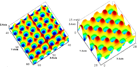
Figure 1: a) A three-dimensional plot of the two-dimensional phase separation potential ${V_{\rm GL}}({\bf r},T)$ viewed from just above the CuO plane. Notice the array of similar potential wells that host rich and poor alternating charge density domains $p({\bf r})$. b) Similar view of the SC amplitudes $\Delta_{d}({\bf r})$ that also follows the same modulation pattern, what is known as pair density waves.

The derived CDW density map that reproduces the measurements of a given compound and the respective ${V_{\rm GL}}$ will be used in the BdG calculations to obtain the SC properties in the next section.

III The BdG superconducting Calculations

To perform the BdG SC approach, we use two results from the CH calculations:

1- The CDW density map $p({\bf r})$.

2- The functional $V_{\rm GL}({\bf r})$ shown in Fig. 1(a)

As mentioned in the introduction, at low temperatures, $V_{\rm GL}({\bf r},T)$ constrains the planar charges in alternating hole-rich and hole-poor domains forming the CDW structure. These alternating densities force the ions to oscillate around new displaced positions as observed by x-ray diffractionChang et al. (2012). They interact back with the holes, leading to a local lattice-mediated hole-hole attraction and Cooper pairs inside the CDW domains, recalling that this possible because the SC coherence length $\xi$ is in general shorter than $\lambda_{CO}$. This pairing interaction is dependent on the CDW hole-rich and hole-poor local concentrations, and it is reasonable to assume that it scales with the localization potential $V_{\rm GL}({\bf r},T)$de Mello (2020).

We use this interaction as a nearest neighbor potential attraction in an extended Hubbard model to calculate the local SC amplitudes $\Delta_{d}({\bf r}_{i})$. This is done by a self-consistent approach that keeps the $p({\bf r}_{i})$ CDW structure constant from the beginning to the end of the calculations following several different experimentsWise et al. (2008); Gomes et al. (2007); Parker et al. (2010); Chang et al. (2012); Miao et al. (2021). This is achieved by changing the local chemical potential $\mu({\bf r}_{i})$ at each iteration until the $\Delta_{d}({\bf r}_{i})$ amplitudes converge and the density map $p({\bf r}_{i})$ is preserved. At the end of the calculations we obtain the original CDW map and the local $d$-wave amplitudes $\Delta_{d}({\bf r}_{i})$ with the same charge modulations ($\lambda_{\rm CO}(p)$) what is known as pair density waves (PDW)de Mello and Sonier (2017). This is shown in Fig. 1(b) for the same compound of Fig. 1(a).

The $\Delta_{d}({\bf r}_{i},p,T)$ local spatial variations imply that global properties like the condensation energies, critical temperatures, and inter-intralayer Josephson coupling, are a function of the average SC amplitudesde Mello (2020, 2021); Santana and de Mello (2022) given by:

$${\left<\Delta_{d}(p,T)\right>}=\sum_{i}^{N}\Delta_{d}({\bf r}_{i},p,T)/N,$$ (3)

where the sum, like in the case of ${\left<V_{\rm GL}(p)\right>}$, is over the N unit cells of a single CuO plane.

IV Josephson Coupling Calculations

We mentioned in the introduction that the CDW structure shown in Fig. 1(a) with its charge domains bounded by the $V_{\rm GL}({\bf r}_{i},p,T)$ potential has some similarities with granular materials. In this case, the charges are bounded to the physical grains by the surface potential and local superconductivity may arise in the interior. Long-range order or supercurrents are a consequence of Josephson tunneling between the grainsKetterson and Song (1999). Although the HTS crystals are not granular in a structural sense, the ubiquitous CDW in these materials led us to suggestde Mello (2012) that they may form an array of mesoscopic Josephson junctions.

Under this assumption, the SC transition develops in two steps when the temperature decreasesKetterson and Song (1999): Firstly, the order parameters with local amplitudes $\Delta_{d}({\bf r}_{i},p,T)$ and phases $\theta_{i}$ arise in each charge CDW domain $``i$”. These localized amplitudes give rise to local Josephson coupling $E_{\rm J}(r_{ij})$ that is proportional to th local supercurrent or th lattice version of the local superfluid densitySpivak and Kivelson (1991) $n_{\rm sc}$, and proportional to the local phase stiffness.

Secondly, upon cooling more, the local phase stiffness increases and eventually overcomes thermal disorder, which leads to a SC transition by long-range phase order. Therefore, we emphasize that the SC critical temperature $T_{\rm c}$ is determined by the competition between thermal disorder and the average planar Josephson energy ${\left<E_{\rm J}(p,T)\right>}$.

These in-plane calculations are the fundamental pillars of the three-dimensional LRO in the whole system, which we infer from transport measurements. For low doping $p$, the $c$-direction resistivity $\rho_{c}$ is $\approx 10^{3}-10^{6}$ larger than the $a$ or $b$-axis resistivity $\rho_{ab}$, a behavior shared also by ${\mathrm{Bi}}_{2}{\mathrm{Sr}}_{2-x}{\mathrm{La}}_{x}{\mathrm{CuO}}_{6+\delta}$Ono and Ando (2003); Komiya et al. (2002). Despite this huge difference, it is surprising that both $\rho_{c}(T)$, and $\rho_{ab}(T)$ fall to zero at the same temperature ($T_{\rm c}$). We have recently argued that the mechanism behind this puzzling behavior may be understood in terms of the planar and weaker out-of-plane average Josephson couplingde Mello (2012), exactly like the weakly coupled XY models.

As explained previouslyde Mello and Sonier (2014), even for $d$-wave amplitudes, it is sufficient to use the Ambegaokar-Baratoff analytical $s$-wave expressionAmbegaokar and Baratoff (1963) averaged over the plane:

$${\left<E_{\rm J}(p,T)\right>}^{X}=\frac{\pi\hbar{\left<\Delta_{d}(p,T)\right>}}{4e^{2}R^{X}_{\rm n}(p)}{\rm tanh}\bigl{[}\frac{\left<\Delta_{d}(p,T)\right>}{2k_{\rm B}T}\bigr{]}.$$ (4)

Where $X=ab$ for planar and $X=c$ for interlayer coupling and $R^{X}_{\rm n}(p,\sim T_{\rm c})$ is the corresponding normal state directional resistance just above $T_{\rm c}$. In our model of an array of Josephson junctions, the current is composed of Cooper pairs tunneling between the CDW domains and by normal carriers or quasiparticle planar currentBruder et al. (1995). For a d-wave HTS near Tc the supercurrent is dominantBruder et al. (1995), which justifies the use of the experimental $R_{\rm n}(T_{\rm c})$ between the charge domains in Eq. 6.

As mentioned, thermal energy causes phase disorder and coherence is achievedde Mello (2012, 2021) at ${\left<E_{\rm J}(p,T_{\rm c})\right>}^{ab}=k_{\rm B}T_{\rm c}$. The smaller planar resistances yield larger $E_{\rm J}^{ab}$ that promote first LRO in the planes, but each plane “$i$” would have its own SC phase $\theta_{i}$ if it was not for the weaker inter-plane $E_{\rm J}^{c}$ coupling. It is similar to a ferromagnet cooled down in the presence of a tiny magnetic field causing all the moments to become aligned.

Thus, the weaker interlayer coupling ${\left<E_{\rm J}(p,T)\right>}^{c}$ connects the planes but leads to only a single-phase $\theta$ at $T\leq T_{\rm c}$ in the whole system, and both $c$ and $ab$ resistivity drop off together despite their orders of magnitude difference.

V Magnetic Penetration depth and resistivity

According to Eq. 4, due to the large difference in the directional resistivities, we expect smaller superfluid densities $n_{\rm sc}$ along the $c$-direction than along the plane, which is confirmed by the $ab$ and $c$-axis penetration depth anisotropyShibauchi et al. (1994); Panagopoulos et al. (2000, 1999). We recall also that the square of the magnetic penetration depth $\lambda$ is inversely proportional to the phase stiffness $\rho_{\rm sc}$Božović et al. (2016) that is proportional to the average Josephson currentSpivak and Kivelson (1991).

Along these lines and in the frame of the L-D modelLawrence and Doniach (1971), Shibauchi et alShibauchi et al. (1994) successfully reproduced their $c$-axis $\lambda_{c}(p)$ measurements. We extend here their approach to account for Josephson current between the CDW charge domains in the CuO planes and use thatde Mello (2020, 2021); Božović et al. (2016) $\lambda^{2}_{X}(p)\propto 1/{\left<E_{\rm J}(p,T)\right>}^{X}$. Therefore, we may write:

$$[\frac{\lambda_{c}(0)}{\lambda_{ab}(0)}]^{2}\propto[\frac{{\left<E_{\rm J}(p,T)\right>}^{ab}}{{\left<E_{\rm J}(p,T)\right>}^{c}}\propto\frac{R^{c}_{\rm n}}{R^{ab}_{\rm n}},$$ (5)

and $R^{c}_{\rm n}=\rho_{c}(T_{\rm c})s$ where $s$ is the distance between the CuO layers in double-plane LSCO crystals is approximately 6.6 $\AA$. This means that $\lambda_{c}(p)$ is dominated by the interplane Josephson current and, extending this idea, $\lambda_{ab}(p)$ is dominated by the planar average coupling ${\left<E_{\rm J}(p,T_{\rm c})\right>}^{ab}$. Therefore, we may write the planar resistivity $R^{ab}_{\rm n}=\rho_{ab}(T_{\rm c})\lambda_{\rm CO}$, since $\lambda_{\rm CO}(p)$ is the distance between the planar CDW domains. Therefore, in a general way,

$$[\frac{\lambda_{c}(0)}{\lambda_{ab}(0)}]^{2}\propto\frac{R^{c}_{\rm n}}{R^{ab}_{\rm n}}\propto\frac{\rho_{c}(T_{\rm c})s}{\rho_{ab}(T_{\rm c})\lambda_{\rm CO}}.$$ (6)

This expression gives the magnetic penetration depths out of the plane and planar ratio in terms of similar resistivities ratio, the planar distance $s$, and the CDW wavelength $\lambda_{\rm CO}$. Notice that there is not any adjustable parameter in Eq. 6 and all quantities have previously been measured.

Some HTS samples with similar doping have comparable resistivities like the La and Y-based compounds studied by Ando et alAndo et al. (2004). When this is the case the above equation shows why the low temperature ratios $\lambda_{c}(p,0)/\lambda_{ab}(p,0)$ for different families of compounds have similar valuesSchneider and Keller (2004). This is the case for a large number of LSCO and HgBa₂CuO_4+x Panagopoulos et al. (2000) samples and they are also comparable with the measurements of $c$-axis grain-aligned orthorhombic YBa₂Cu₃O_7-δ (YBCO) with $\delta=0.0,0.3,$ and $0.43$Panagopoulos et al. (1998). The quantitative explanation of these data and their connection with the $\rho_{c}(T_{\rm c})/\rho_{ab}(T_{\rm c})$ is one of the main motivations of our present calculations.

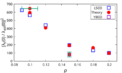
Figure 2: Six LSCO $[\lambda_{c}(0)/\lambda_{ab}(0)]^{2}$ experimental points Shibauchi et al. (1994); Panagopoulos et al. (2000) and one optimal YBCO-aligned powder in magnetic field with 30% uncertaintyPanagopoulos et al. (1998) represented by the error bar. They are together with the calculations from Eq. 6 which use the CDW wavelengthsComin and Damascelli (2016) $\lambda_{CO}(p)$ and the respective resistivity ratiosKimura et al. (1992); Nakamura and Uchida (1993) listed in Tables 1 and 2. For $p=0.09$ we use the resistivities of $p=0.10\pm 0.01$ from Ref. Nakamura and Uchida, 1993 as explained in the text.

On the other hand, most of the data on directional $\lambda_{X}(0)$ and $\rho_{X}(T_{\rm c})$ with the same doping $p$ were performed a long time ago with LSCO crystals in order to understand the anisotropies in HTS. Nowadays there are single crystals of many other materials but since the anisotropies are already established these measurements are not remade. The difficulty to fabricate single crystals in the earlier days of HTS is the reason why data on other materials are practically nonexistent. In most cases, whenever there are data on $\lambda_{c}(0)/\lambda_{ab}(0)$, it is not accompanied by $\rho_{c}(T_{\rm c})/\rho_{ab}(T_{\rm c})$ that is needed by our Eq. 6. Nevertheless, we list in Table 1 the available data on LSCO for $(\lambda_{c}(0)/\lambda_{ab}(0))^{2}$Shibauchi et al. (1994); Panagopoulos et al. (2000) ratios and $\rho_{c}(T_{\rm c})/\rho_{ab}(T_{\rm c})$Kimura et al. (1992); Nakamura and Uchida (1993). The case of $(\lambda_{c}(0.09)/\lambda_{ab}(0.09))^{2}$, the resistivity data of different groups have discrepant results and we used $\rho_{c}/\rho_{ab}(0.10\pm 0.01)$ from Ref. Nakamura and Uchida, 1993 (marked with a star). With these data and the respective CDW wavelengths $\lambda_{CO}(p)$ that enters in Eq. 6 for the planar $R^{ab}_{\rm n}$, we calculated the magnetic penetration depth ratio. The experimental results and our estimates are plotted together for comparison in Fig. 2, and listed in columns two and five of Table 1.

Table 1: Data and calculations for LSCO. The first column is hole density per unit cell. Second is the $(\lambda_{c}(0)/\lambda_{ab}(0))^{2}$ measurements of Shibauchi et alShibauchi et al. (1994) and Panagopoulos et alPanagopoulos et al. (2000). Third is the $\rho_{c}(T_{\rm c})/\rho_{ab}(T_{\rm c})$Kimura et al. (1992); Nakamura and Uchida (1993) resistivity ratios. The fourth is $\lambda_{CO}$ in units of the lattice parameter $a_{0}\approx 3.78\AA$ measured by REXSComin and Damascelli (2016). The last column is the calculations from Eq. 6 with $s=6.6\AA$ that should match the magnetic penetration depth ratio of the second column. The case of $(\lambda_{c}(0.09)/\lambda_{ab}(0.09))^{2}$, the resistivity data of different groups conflict and we used the $p=0.10\pm 0.01$ resistivity ratio $\rho_{c}/\rho_{ab}$ from Ref. Nakamura and Uchida, 1993 (marked with a star).

Sample	$(\lambda_{c}(0)/\lambda_{ab}(0))^{2}$	$\rho_{c}/\rho_{ab}(T_{\rm c})$	$\lambda_{CO}(\AA)$	$\rho_{c}s/\rho_{ab}\lambda_{CO}$
p = 0.09	625	2070*	5.6 $a_{0}$	645*
p = 0.10	$\propto$ 564	1714	5.0 $a_{0}$	595
p = 0.12	441	1000	4.25 $a_{0}$	408
p = 0.15	196	433	3.9 $a_{0}$	193
p = 0.18	132	300	3.7 $a_{0}$	164
p = 0.20	100	200	3.6 $a_{0}$	97

There are also some data on $\lambda_{c}(0)/\lambda_{ab}(0)$ in magnetic aligned powder of YBa₂Cu₃O_7-δPanagopoulos et al. (1998) (YBCO) that contains some uncertainty up to 30% in the $c$-axis but provides good estimates of this ratio. Similarly, we use new anisotropic $\rho_{c}(T_{\rm c})/\rho_{ab}(T_{\rm c})$ optimal data on thin films of YBCO grown on an off-axis cut SrTiO3 substrateHeine et al. (2021). Combining these data, we can apply Eq. 6 to this near optimal compound and the calculation is very close to the YBCO experimental result as shown in Fig. 2 and in Table 2.

Table 2: Data and calculations for optimal YBCO similar to Table 1. The uncertainty of 30% in $(\lambda_{c}(0)/\lambda_{ab}(0))^{2}$ is due to the $c$-axis alignment uncertainty of the powders. For YBCO, the distance between two planes is $s=5.84\AA$ and for optimal dopingComin and Damascelli (2016) $\lambda_{CO}=3.12a_{0}$.

Sample	$(\lambda_{c}(0)/\lambda_{ab}(0))^{2}$	$\rho_{c}(T_{\rm c})/\rho_{ab}(T_{\rm c})$	$\lambda_{CO}(\AA)$	$\rho_{c}s/\rho_{ab}\lambda_{CO}$
p = 0.15	81 $\pm$ 25	167	3.9 $a_{0}$	81.5

VI Conclusion

In this paper, we generalize the ideas of ILT and L-D models to account also for Josephson coupling between the mesoscopic CDW domains or blocks. The in-plane average Josephson energy is much larger than the interlayer coupling, proportional to $1/\lambda_{ab}^{2}$ and to the thermal energy at the critical temperature $T_{\rm c}$. Therefore the SC properties are almost entirely dependent on the planar Josephson coupling in opposition to the old ILT model, which depended on the interlayer Josephson tunneling. Our approach yields values of $\lambda_{ab}$ at least one order of magnitude larger than $\lambda_{c}$, which gives some insights why measurementsMoler et al. (1998) of $\lambda_{c}$ gave much smaller condensation energy than the old ILT predictionsLeggett (1996).

Furthermore, we derive a new equation relating the magnetic penetration depths $(\lambda_{c}(0)/\lambda_{ab}(0))^{2}$ with the resistivities $[\rho_{c}(T_{\rm c})s]/[\rho_{ab}(T_{\rm c})\lambda_{\rm CO}]$ (Eq. 6), which is in agreement with many measurements without any adjustable parameter. Nowadays there are better single crystals of many materials but since the anisotropies are already established these combined measurements($\rho_{X}(T_{\rm c})$ and $(\lambda_{X}(0)$) on a single sample are not anymore explored. However, Eq. 6 provides new motivation for more precise tests in future experiments with modern pristine HTS crystals.

VII acknowledgements

We acknowledge partial support from the Brazilian agencies CNPq and FAPERJ.

References

- Clem (1989) J. R. Clem, Physica C 162-164, 1137 (1989).
- Clem (1991) J. R. Clem, Phys. Rev. B 43, 7837 (1991).
- Chakravarty et al. (1993) S. Chakravarty, A. Sudbo, P. W. Anderson, and S. Strong, Science , 337+ (1993), 5119.
- Anderson (1995) P. Anderson, Science 268, 1154 (1995).
- Leggett (1996) A. J. Leggett, Science 274, 587 (1996).
- Lawrence and Doniach (1971) W. Lawrence and S. Doniach, in Proceedings of the Twelfth International Conference on Low Temperature Physics (Ed. by E. Kanda, Academic Press of Japan, Kyoto, Japan, 1971) p. 361.
- Shibauchi et al. (1994) T. Shibauchi, H. Kitano, K. Uchinokura, A. Maeda, T. Kimura, and K. Kishio, Phys. Rev. Lett. 72, 2263 (1994).
- Moler et al. (1998) K. A. Moler, J. R. Kirtley, D. Hinks, T. Li, and M. Xu, Science 279, 1193 (1998).
- Anderson (1998) P. W. Anderson, Science 279, 1196+ (1998), 5354.
- Tranquada et al. (1995) J. M. Tranquada, B. J. Sternlieb, J. D. Axe, Y. Nakamura, and S. Uchida, Nature 375, 561 (1995).
- Lang et al. (2002) K. M. Lang, V. Madhavan, J. E. Hoffman, E. W. Hudson, H. Eisaki, S. Uchida, and J. C. Davis, Nature 415, 412 (2002).
- Fischer et al. (2007) O. Fischer, M. Kugler, I. Maggio-Aprile, C. Berthod, and C. Renner, Rev. Mod. Phys. 79, 353 (2007).
- Comin and Damascelli (2016) R. Comin and A. Damascelli, Ann. Rev. of Cond. Mat. Phys. 7, 369 (2016).
- Wise et al. (2008) W. D. Wise et al., Nature Physics 4, 696 (2008).
- Gomes et al. (2007) K. K. Gomes et al., Nature 447, 569 (2007).
- Parker et al. (2010) C. V. Parker, P. Aynajian, E. H. da Silva Neto, A. Pushp, S. Ono, J. Wen, Z. Xu, G. Gu, and A. Yazdani, Nature 468, 677 (2010).
- He et al. (2014) Y. He, Y. Yin, M. Zech, A. Soumyanarayanan, M. M. Yee, T. Williams, M. C. Boyer, K. Chatterjee, W. D. Wise, I. Zeljkovic, T. Kondo, T. Takeuchi, H. Ikuta, P. Mistark, R. S. Markiewicz, A. Bansil, S. Sachdev, E. W. Hudson, and J. E. Hoffman, Science 344, 608 (2014).
- (18) E. H. da Silva Neto, M. Minola, B. Yu, W. Tabis, M. Bluschke, D. Unruh, H. Suzuki, Y. Li, G. Yu, D. Betto, K. Kummer, F. Yakhou, N. B. Brookes, M. Le Tacon, M. Greven, B. Keimer, and A. Damascelli, .
- Wu et al. (2017) J. Wu, A. T. Bollinger, X. He, and I. Božović, Nature 547, 432 (2017).
- Chen et al. (2019) S.-D. Chen, M. Hashimoto, Y. He, D. Song, K.-J. Xu, J.-F. He, T. P. Devereaux, H. Eisaki, D.-H. Lu, J. Zaanen, and Z.-X. Shen, Science 366, 1099 (2019).
- Fei et al. (2019) Y. Fei, Y. Zheng, K. Bu, W. Zhang, Y. Ding, X. Zhou, and Y. Yin, Science China Physics, Mechanics & Astronomy 63, 227411 (2019).
- Miao et al. (2021) H. Miao, G. Fabbris, R. J. Koch, D. G. Mazzone, C. S. Nelson, R. Acevedo-Esteves, G. D. Gu, Y. Li, T. Yilimaz, K. Kaznatcheev, E. Vescovo, M. Oda, T. Kurosawa, N. Momono, T. Assefa, I. K. Robinson, E. S. Bozin, J. M. Tranquada, P. D. Johnson, and M. P. M. Dean, npj Quantum Materials 6, 31 (2021).
- de Mello (2012) E. V. L. de Mello, Europhys. Lett. 99, 37003 (2012).
- de Mello and Sonier (2014) E. V. L. de Mello and J. E. Sonier, J. Phys.: Condens. Matter 26, 492201 (2014).
- de Mello and Sonier (2017) E. V. L. de Mello and J. E. Sonier, Phys. Rev. B 95, 184520 (2017).
- de Mello (2020) E. V. de Mello, J. Phys.: Condens. Matter 32, 40LT02 (2020).
- Santana and de Mello (2022) H. S. Santana and E. de Mello, Phys. Rev. B 105, 134513 (2022).
- Spivak and Kivelson (1991) B. I. Spivak and S. A. Kivelson, Phys. Rev. B 43, 3740 (1991).
- Božović et al. (2016) I. Božović, X. He, J. Wu, and A. T. Bollinger, Nature 536, 309 (2016).
- Panagopoulos et al. (2000) C. Panagopoulos, J. R. Cooper, T. Xiang, Y. S. Wang, and C. W. Chu, Phys. Rev. B 61, R3808 (2000).
- Kimura et al. (1992) T. Kimura, K. Kishio, T. Kobayashi, Y. Nakayama, N. Motohira, K. Kitazawa, and K. Yamafuji, Physica C: Superconductivity 192, 247 (1992).
- Nakamura and Uchida (1993) Y. Nakamura and S. Uchida, Phys. Rev. B 47, 8369 (1993).
- de Mello and da Silveira Filho (2005) E. de Mello and O. T. da Silveira Filho, Physica A 347, 429 (2005).
- de Mello et al. (2009) E. V. L. de Mello, R. B. Kasal, and C. A. C. Passos, J. Phys.: Condens. Matter 21, 235701 (2009).
- Bray (1994) A. Bray, Adv. Phys. 43, 357 (1994).
- de Mello (2021) E. V. L. de Mello, J. of Phys.: Cond. Matter 33, 145503 (2021).
- Chang et al. (2012) J. Chang, E. Blackburn, T. Holmes, N. B. Christensen, J. Larsen, J. Mesot, R. Liang, D. A. Bonn, W. N. Hardy, A. Watenphul, M. V. Zimmermann, E. M. Forgan, and S. M. Hayden, Nature Physics 8, 871 (2012).
- Ketterson and Song (1999) J. B. Ketterson and S. Song, Superconductivity (Cambridge University Press, London, 1999).
- Ono and Ando (2003) S. Ono and Y. Ando, Phys. Rev. B 67, 104512 (2003).
- Komiya et al. (2002) S. Komiya, Y. Ando, X. F. Sun, and A. N. Lavrov, Phys. Rev. B 65, 214535 (2002).
- Ambegaokar and Baratoff (1963) V. Ambegaokar and A. Baratoff, Phys. Rev. Lett. 10, 486 (1963).
- Bruder et al. (1995) C. Bruder, A. van Otterlo, and G. T. Zimanyi, Phys. Rev. B 51, 12904 (1995).
- Panagopoulos et al. (1999) C. Panagopoulos, J. L. Tallon, and T. Xiang, Phys. Rev. B 59, R6635 (1999).
- Ando et al. (2004) Y. Ando, S. Komiya, K. Segawa, S. Ono, and Y. Kurita, Phys. Rev. Lett. 93, 267001 (2004).
- Schneider and Keller (2004) T. Schneider and H. Keller, New Journal of Physics 6, 144 (2004).
- Panagopoulos et al. (1998) C. Panagopoulos, J. R. Cooper, and T. Xiang, Phys. Rev. B 57, 13422 (1998).
- Heine et al. (2021) G. Heine, W. Lang, R. Rössler, and J. D. Pedarnig, Nanomaterials 11 (2021), 10.3390/nano11030675.