On Parsing as Tagging

Afra Amini    Ryan Cotterell
$\{$afra.amini, ryan.cotterell$\}$@inf.ethz.ch
[Uncaptioned image]
Abstract

There have been many proposals to reduce constituency parsing to tagging in the literature. To better understand what these approaches have in common, we cast several existing proposals into a unifying pipeline consisting of three steps: linearization, learning, and decoding. In particular, we show how to reduce tetratagging, a state-of-the-art constituency tagger, to shift–reduce parsing by performing a right-corner transformation on the grammar and making a specific independence assumption. Furthermore, we empirically evaluate our taxonomy of tagging pipelines with different choices of linearizers, learners, and decoders. Based on the results in English and a set of 8 typologically diverse languages, we conclude that the linearization of the derivation tree and its alignment with the input sequence is the most critical factor in achieving accurate taggers.

[Uncaptioned image]

https://github.com/rycolab/parsing-as-tagging

Refer to caption
Figure 1: We subdivide parsing-as-tagging schemes into three steps: 1) linearization, 2) learning, and 3) decoding. The figure depicts how subdivision affects the parsing of the sentence She enjoys reading papers with pre-order linearization.

1 Introduction

The automatic syntactic analysis of natural language text is an important problem in natural language processing (NLP). Due to the ambiguity present in natural language, many parsers for natural language are statistical in nature, i.e., they provide a probability distribution over syntactic analyses for a given input sequence. A common design pattern for natural language parsers is to re-purpose tools from formal language theory that were often designed for compiler construction (Aho and Ullman, 1972), to construct probability distributions over derivation trees (syntactic analyses). Indeed, one of the most commonly deployed parsers in NLP is a statistical version of the classic shift–reduce parser, which has been widely applied in constituency parsing (Sagae and Lavie, 2005; Zhang and Clark, 2009; Zhu et al., 2013), dependency parsing (Fraser, 1989; Yamada and Matsumoto, 2003; Nivre, 2004), and even for the parsing of more exotic formalisms, e.g., CCG parsing (Zhang and Clark, 2011; Xu et al., 2014).

Another relatively recent trend in statistical parsing is the idea of reducing parsing to tagging (Gómez-Rodríguez and Vilares, 2018; Strzyz et al., 2019; Vilares et al., 2019; Vacareanu et al., 2020; Gómez-Rodríguez et al., 2020; Kitaev and Klein, 2020). There are a number of motivations behind this reduction. For instance, Kitaev and Klein (2020) motivate tetratagging, their novel constituency parsing-as-tagging scheme, by its ability to parallelize the computation during training and to minimize task-specific modeling. The proposed taggers in the literature are argued to exhibit the right balance in the trade-off between accuracy and efficiency. Nevertheless, there are several ways to cast parsing as a tagging problem, and the relationship of each of these ways to transition-based parsing remains underdeveloped.

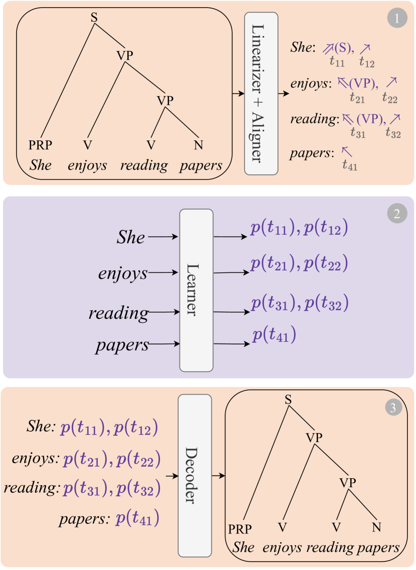
To better understand the relationship between parsing as tagging and transition-based parsing, we identify a common pipeline that many parsing-as-tagging approaches seem to follow. This pipeline, as shown in Fig. 1, consists of three steps: linearization, learning, and decoding. Furthermore, we demonstrate that Kitaev and Klein’s (2020) tetratagging may be derived under two additional assumptions on a classic shift–reduce parser: (i) a right-corner transform in the linearization step and (ii) factored scoring of the rules in the learning step. We find that (i) leads to better alignment with the input sequence, while (ii) leads to parallel execution.

In light of these findings, we propose a taxonomy of parsing-as-tagging schemes based on different choices of linearizations, learners, and decoders. Furthermore, we empirically evaluate the effect that the different choice points have on the performance of the resulting model. Based on experimental results, one of the most important factors in achieving the best-performing tagger is the order in which the linearizer enumerates the tree and the alignment between the tags and the input sequence. We show that taggers with in-order linearization are the most accurate parsers, followed by their pre-order and post-order counterparts, respectively.

Finally, we argue that the effect of the linearization step on parsing performance can be explained by the deviation between the resulting tag sequence and the input sequence, which should be minimized. We theoretically show that in-order linearizers always generate tag sequences with zero deviation. On the other hand, the deviation of pre- and post-order linearizations in the worst case grows in order of sentence length. Empirically, experiments on a set of 9 typologically diverse languages show that the deviation varies across languages and negatively correlates with parsing performance. Indeed, we find that the deviation appears to be the most important factor in predicting parser performance.

Linearizations
𝐚𝐰presuperscriptsubscript𝐚𝐰pre\color[rgb]{0,0,0}\definecolor[named]{pgfstrokecolor}{rgb}{0,0,0}\pgfsys@color@gray@stroke{0}\pgfsys@color@gray@fill{0}{\mathbf{a}_{{\color[rgb]{0,0,0}\definecolor[named]{pgfstrokecolor}{rgb}{0,0,0}\pgfsys@color@gray@stroke{0}\pgfsys@color@gray@fill{0}\mathbf{w}}}^{\text{pre}}} Φ𝐰pre(d𝐰)superscriptsubscriptΦ𝐰presubscript𝑑𝐰\color[rgb]{0,0,0}\definecolor[named]{pgfstrokecolor}{rgb}{0,0,0}\pgfsys@color@gray@stroke{0}\pgfsys@color@gray@fill{0}\Phi_{{\color[rgb]{0,0,0}\definecolor[named]{pgfstrokecolor}{rgb}{0,0,0}\pgfsys@color@gray@stroke{0}\pgfsys@color@gray@fill{0}\mathbf{w}}}^{\text{pre}}({\color[rgb]{0,0,0}\definecolor[named]{pgfstrokecolor}{rgb}{0,0,0}\pgfsys@color@gray@stroke{0}\pgfsys@color@gray@fill{0}d_{{\color[rgb]{0,0,0}\definecolor[named]{pgfstrokecolor}{rgb}{0,0,0}\pgfsys@color@gray@stroke{0}\pgfsys@color@gray@fill{0}\mathbf{w}}}}) Φ𝐰post(d𝐰)superscriptsubscriptΦ𝐰postsubscript𝑑𝐰\color[rgb]{0,0,0}\definecolor[named]{pgfstrokecolor}{rgb}{0,0,0}\pgfsys@color@gray@stroke{0}\pgfsys@color@gray@fill{0}\Phi_{{\color[rgb]{0,0,0}\definecolor[named]{pgfstrokecolor}{rgb}{0,0,0}\pgfsys@color@gray@stroke{0}\pgfsys@color@gray@fill{0}\mathbf{w}}}^{\text{post}}({\color[rgb]{0,0,0}\definecolor[named]{pgfstrokecolor}{rgb}{0,0,0}\pgfsys@color@gray@stroke{0}\pgfsys@color@gray@fill{0}d_{{\color[rgb]{0,0,0}\definecolor[named]{pgfstrokecolor}{rgb}{0,0,0}\pgfsys@color@gray@stroke{0}\pgfsys@color@gray@fill{0}\mathbf{w}}}}) Φ𝐰in(d𝐰)superscriptsubscriptΦ𝐰insubscript𝑑𝐰\color[rgb]{0,0,0}\definecolor[named]{pgfstrokecolor}{rgb}{0,0,0}\pgfsys@color@gray@stroke{0}\pgfsys@color@gray@fill{0}\Phi_{{\color[rgb]{0,0,0}\definecolor[named]{pgfstrokecolor}{rgb}{0,0,0}\pgfsys@color@gray@stroke{0}\pgfsys@color@gray@fill{0}\mathbf{w}}}^{\text{in}}({\color[rgb]{0,0,0}\definecolor[named]{pgfstrokecolor}{rgb}{0,0,0}\pgfsys@color@gray@stroke{0}\pgfsys@color@gray@fill{0}d_{{\color[rgb]{0,0,0}\definecolor[named]{pgfstrokecolor}{rgb}{0,0,0}\pgfsys@color@gray@stroke{0}\pgfsys@color@gray@fill{0}\mathbf{w}}}})
reduce(SPRPVP)reduceSPRPVP{\scriptstyle{\color[rgb]{0,0,0}\definecolor[named]{pgfstrokecolor}{rgb}{0,0,0}\pgfsys@color@gray@stroke{0}\pgfsys@color@gray@fill{0}\textsc{reduce}}(\mathrm{S}\rightarrow\mathrm{PRP}\,\mathrm{VP})} \Circled1:(S)\Circled{1}:{\color[rgb]{0,0,0}\definecolor[named]{pgfstrokecolor}{rgb}{0,0,0}\pgfsys@color@gray@stroke{0}\pgfsys@color@gray@fill{0}\mathrel{\rotatebox[origin={c}]{45.0}{$\Rightarrow$}}}(\mathrm{S}) \Circled2::\Circled2\Circled{2}:{\color[rgb]{0,0,0}\definecolor[named]{pgfstrokecolor}{rgb}{0,0,0}\pgfsys@color@gray@stroke{0}\pgfsys@color@gray@fill{0}\mathrel{\rotatebox[origin={c}]{45.0}{$\rightarrow$}}} \Circled2::\Circled2\Circled{2}:{\color[rgb]{0,0,0}\definecolor[named]{pgfstrokecolor}{rgb}{0,0,0}\pgfsys@color@gray@stroke{0}\pgfsys@color@gray@fill{0}\mathrel{\rotatebox[origin={c}]{45.0}{$\rightarrow$}}}
shift(PRPShe)shiftPRPShe{\scriptstyle{\color[rgb]{0,0,0}\definecolor[named]{pgfstrokecolor}{rgb}{0,0,0}\pgfsys@color@gray@stroke{0}\pgfsys@color@gray@fill{0}\textsc{shift}}(\mathrm{PRP}\rightarrow\textit{She})} \Circled2::\Circled2\Circled{2}:{\color[rgb]{0,0,0}\definecolor[named]{pgfstrokecolor}{rgb}{0,0,0}\pgfsys@color@gray@stroke{0}\pgfsys@color@gray@fill{0}\mathrel{\rotatebox[origin={c}]{45.0}{$\rightarrow$}}} \Circled4::\Circled4\Circled{4}:{\color[rgb]{0,0,0}\definecolor[named]{pgfstrokecolor}{rgb}{0,0,0}\pgfsys@color@gray@stroke{0}\pgfsys@color@gray@fill{0}\mathrel{\rotatebox[origin={c}]{45.0}{$\rightarrow$}}} \Circled1:(S)\Circled{1}:{\color[rgb]{0,0,0}\definecolor[named]{pgfstrokecolor}{rgb}{0,0,0}\pgfsys@color@gray@stroke{0}\pgfsys@color@gray@fill{0}\mathrel{\rotatebox[origin={c}]{45.0}{$\Rightarrow$}}}(\mathrm{S})
reduce(VPVVP)reduceVPVVP{\scriptstyle{\color[rgb]{0,0,0}\definecolor[named]{pgfstrokecolor}{rgb}{0,0,0}\pgfsys@color@gray@stroke{0}\pgfsys@color@gray@fill{0}\textsc{reduce}}(\mathrm{VP}\rightarrow\mathrm{V}\,\mathrm{VP})} \Circled3:(VP)\Circled{3}:{\color[rgb]{0,0,0}\definecolor[named]{pgfstrokecolor}{rgb}{0,0,0}\pgfsys@color@gray@stroke{0}\pgfsys@color@gray@fill{0}\mathrel{\rotatebox[origin={c}]{135.0}{$\Rightarrow$}}}(\mathrm{VP}) \Circled6::\Circled6\Circled{6}:{\color[rgb]{0,0,0}\definecolor[named]{pgfstrokecolor}{rgb}{0,0,0}\pgfsys@color@gray@stroke{0}\pgfsys@color@gray@fill{0}\mathrel{\rotatebox[origin={c}]{45.0}{$\rightarrow$}}} \Circled4::\Circled4\Circled{4}:{\color[rgb]{0,0,0}\definecolor[named]{pgfstrokecolor}{rgb}{0,0,0}\pgfsys@color@gray@stroke{0}\pgfsys@color@gray@fill{0}\mathrel{\rotatebox[origin={c}]{45.0}{$\rightarrow$}}}
shift(Venjoys)shiftVenjoys{\scriptstyle{\color[rgb]{0,0,0}\definecolor[named]{pgfstrokecolor}{rgb}{0,0,0}\pgfsys@color@gray@stroke{0}\pgfsys@color@gray@fill{0}\textsc{shift}}(\mathrm{V}\rightarrow\textit{enjoys})} \Circled4::\Circled4\Circled{4}:{\color[rgb]{0,0,0}\definecolor[named]{pgfstrokecolor}{rgb}{0,0,0}\pgfsys@color@gray@stroke{0}\pgfsys@color@gray@fill{0}\mathrel{\rotatebox[origin={c}]{45.0}{$\rightarrow$}}} \Circled7::\Circled7\Circled{7}:{\color[rgb]{0,0,0}\definecolor[named]{pgfstrokecolor}{rgb}{0,0,0}\pgfsys@color@gray@stroke{0}\pgfsys@color@gray@fill{0}\mathrel{\rotatebox[origin={c}]{135.0}{$\rightarrow$}}} \Circled3:(VP)\Circled{3}:{\color[rgb]{0,0,0}\definecolor[named]{pgfstrokecolor}{rgb}{0,0,0}\pgfsys@color@gray@stroke{0}\pgfsys@color@gray@fill{0}\mathrel{\rotatebox[origin={c}]{135.0}{$\Rightarrow$}}}(\mathrm{VP})
reduce(VPVN)reduceVPVN{\scriptstyle{\color[rgb]{0,0,0}\definecolor[named]{pgfstrokecolor}{rgb}{0,0,0}\pgfsys@color@gray@stroke{0}\pgfsys@color@gray@fill{0}\textsc{reduce}}(\mathrm{VP}\rightarrow\mathrm{V}\,\mathrm{N})} \Circled5:(VP)\Circled{5}:{\color[rgb]{0,0,0}\definecolor[named]{pgfstrokecolor}{rgb}{0,0,0}\pgfsys@color@gray@stroke{0}\pgfsys@color@gray@fill{0}\mathrel{\rotatebox[origin={c}]{135.0}{$\Rightarrow$}}}(\mathrm{VP}) \Circled5:(VP)\Circled{5}:{\color[rgb]{0,0,0}\definecolor[named]{pgfstrokecolor}{rgb}{0,0,0}\pgfsys@color@gray@stroke{0}\pgfsys@color@gray@fill{0}\mathrel{\rotatebox[origin={c}]{135.0}{$\Rightarrow$}}}(\mathrm{VP}) \Circled6::\Circled6\Circled{6}:{\color[rgb]{0,0,0}\definecolor[named]{pgfstrokecolor}{rgb}{0,0,0}\pgfsys@color@gray@stroke{0}\pgfsys@color@gray@fill{0}\mathrel{\rotatebox[origin={c}]{45.0}{$\rightarrow$}}}
shift(Vreading)shiftVreading{\scriptstyle{\color[rgb]{0,0,0}\definecolor[named]{pgfstrokecolor}{rgb}{0,0,0}\pgfsys@color@gray@stroke{0}\pgfsys@color@gray@fill{0}\textsc{shift}}(\mathrm{V}\rightarrow\textit{reading})} \Circled6::\Circled6\Circled{6}:{\color[rgb]{0,0,0}\definecolor[named]{pgfstrokecolor}{rgb}{0,0,0}\pgfsys@color@gray@stroke{0}\pgfsys@color@gray@fill{0}\mathrel{\rotatebox[origin={c}]{45.0}{$\rightarrow$}}} \Circled3:(VP)\Circled{3}:{\color[rgb]{0,0,0}\definecolor[named]{pgfstrokecolor}{rgb}{0,0,0}\pgfsys@color@gray@stroke{0}\pgfsys@color@gray@fill{0}\mathrel{\rotatebox[origin={c}]{135.0}{$\Rightarrow$}}}(\mathrm{VP}) \Circled5:(VP)\Circled{5}:{\color[rgb]{0,0,0}\definecolor[named]{pgfstrokecolor}{rgb}{0,0,0}\pgfsys@color@gray@stroke{0}\pgfsys@color@gray@fill{0}\mathrel{\rotatebox[origin={c}]{135.0}{$\Rightarrow$}}}(\mathrm{VP})
shift(Npapers)shiftNpapers{\scriptstyle{\color[rgb]{0,0,0}\definecolor[named]{pgfstrokecolor}{rgb}{0,0,0}\pgfsys@color@gray@stroke{0}\pgfsys@color@gray@fill{0}\textsc{shift}}(\mathrm{N}\rightarrow\textit{papers})} \Circled7::\Circled7\Circled{7}:{\color[rgb]{0,0,0}\definecolor[named]{pgfstrokecolor}{rgb}{0,0,0}\pgfsys@color@gray@stroke{0}\pgfsys@color@gray@fill{0}\mathrel{\rotatebox[origin={c}]{135.0}{$\rightarrow$}}} \Circled1:(S)\Circled{1}:{\color[rgb]{0,0,0}\definecolor[named]{pgfstrokecolor}{rgb}{0,0,0}\pgfsys@color@gray@stroke{0}\pgfsys@color@gray@fill{0}\mathrel{\rotatebox[origin={c}]{45.0}{$\Rightarrow$}}}(\mathrm{S}) \Circled7::\Circled7\Circled{7}:{\color[rgb]{0,0,0}\definecolor[named]{pgfstrokecolor}{rgb}{0,0,0}\pgfsys@color@gray@stroke{0}\pgfsys@color@gray@fill{0}\mathrel{\rotatebox[origin={c}]{135.0}{$\rightarrow$}}}
Derivation Tree: d𝐰subscript𝑑𝐰{\color[rgb]{0,0,0}\definecolor[named]{pgfstrokecolor}{rgb}{0,0,0}\pgfsys@color@gray@stroke{0}\pgfsys@color@gray@fill{0}d_{{\color[rgb]{0,0,0}\definecolor[named]{pgfstrokecolor}{rgb}{0,0,0}\pgfsys@color@gray@stroke{0}\pgfsys@color@gray@fill{0}\mathbf{w}}}}
{forest} for tree=myleaf/.style=label=[align=center]below:#1 [$\mathrm{S}^{\Circled{1}}$ [$\mathrm{PRP}^{\Circled{2}}$[She] ] [$\mathrm{VP}^{\Circled{3}}$ [$\mathrm{V}^{\Circled{4}}$[enjoys] ] [$\mathrm{VP}^{\Circled{5}}$ [$\mathrm{V}^{\Circled{6}}$[reading] ] [$\mathrm{N}^{\Circled{7}}$[papers] ] ] ] ]
Table 1: Examples of different linearizations for the derivation tree of the sentence She enjoys reading papers. Note that 𝐚𝐰presuperscriptsubscript𝐚𝐰pre\color[rgb]{0,0,0}\definecolor[named]{pgfstrokecolor}{rgb}{0,0,0}\pgfsys@color@gray@stroke{0}\pgfsys@color@gray@fill{0}{\mathbf{a}_{{\color[rgb]{0,0,0}\definecolor[named]{pgfstrokecolor}{rgb}{0,0,0}\pgfsys@color@gray@stroke{0}\pgfsys@color@gray@fill{0}\mathbf{w}}}^{\text{pre}}} is the action sequence of a shift–reduce parser, Φ𝐰pre(d𝐰)superscriptsubscriptΦ𝐰presubscript𝑑𝐰\color[rgb]{0,0,0}\definecolor[named]{pgfstrokecolor}{rgb}{0,0,0}\pgfsys@color@gray@stroke{0}\pgfsys@color@gray@fill{0}\Phi_{{\color[rgb]{0,0,0}\definecolor[named]{pgfstrokecolor}{rgb}{0,0,0}\pgfsys@color@gray@stroke{0}\pgfsys@color@gray@fill{0}\mathbf{w}}}^{\text{pre}}({\color[rgb]{0,0,0}\definecolor[named]{pgfstrokecolor}{rgb}{0,0,0}\pgfsys@color@gray@stroke{0}\pgfsys@color@gray@fill{0}d_{{\color[rgb]{0,0,0}\definecolor[named]{pgfstrokecolor}{rgb}{0,0,0}\pgfsys@color@gray@stroke{0}\pgfsys@color@gray@fill{0}\mathbf{w}}}}) is the pre-order linearization, Φ𝐰post(d𝐰)superscriptsubscriptΦ𝐰postsubscript𝑑𝐰\color[rgb]{0,0,0}\definecolor[named]{pgfstrokecolor}{rgb}{0,0,0}\pgfsys@color@gray@stroke{0}\pgfsys@color@gray@fill{0}\Phi_{{\color[rgb]{0,0,0}\definecolor[named]{pgfstrokecolor}{rgb}{0,0,0}\pgfsys@color@gray@stroke{0}\pgfsys@color@gray@fill{0}\mathbf{w}}}^{\text{post}}({\color[rgb]{0,0,0}\definecolor[named]{pgfstrokecolor}{rgb}{0,0,0}\pgfsys@color@gray@stroke{0}\pgfsys@color@gray@fill{0}d_{{\color[rgb]{0,0,0}\definecolor[named]{pgfstrokecolor}{rgb}{0,0,0}\pgfsys@color@gray@stroke{0}\pgfsys@color@gray@fill{0}\mathbf{w}}}}) is the post-order linearization, and Φ𝐰in(d𝐰)superscriptsubscriptΦ𝐰insubscript𝑑𝐰\color[rgb]{0,0,0}\definecolor[named]{pgfstrokecolor}{rgb}{0,0,0}\pgfsys@color@gray@stroke{0}\pgfsys@color@gray@fill{0}\Phi_{{\color[rgb]{0,0,0}\definecolor[named]{pgfstrokecolor}{rgb}{0,0,0}\pgfsys@color@gray@stroke{0}\pgfsys@color@gray@fill{0}\mathbf{w}}}^{\text{in}}({\color[rgb]{0,0,0}\definecolor[named]{pgfstrokecolor}{rgb}{0,0,0}\pgfsys@color@gray@stroke{0}\pgfsys@color@gray@fill{0}d_{{\color[rgb]{0,0,0}\definecolor[named]{pgfstrokecolor}{rgb}{0,0,0}\pgfsys@color@gray@stroke{0}\pgfsys@color@gray@fill{0}\mathbf{w}}}}) is the in-order linearization (tetratagger).

2 Preliminaries

Before diving into the details of parsing as tagging, we introduce the notation that is used throughout the paper. We assume that we have a weighted grammar in Chomsky normal form 𝔊=𝒩,S,Σ,𝔊𝒩SΣ{\color[rgb]{0,0,0}\definecolor[named]{pgfstrokecolor}{rgb}{0,0,0}\pgfsys@color@gray@stroke{0}\pgfsys@color@gray@fill{0}\mathfrak{G}}=\langle{\color[rgb]{0,0,0}\definecolor[named]{pgfstrokecolor}{rgb}{0,0,0}\pgfsys@color@gray@stroke{0}\pgfsys@color@gray@fill{0}\mathcal{N}},\mathrm{S},{\color[rgb]{0,0,0}\definecolor[named]{pgfstrokecolor}{rgb}{0,0,0}\pgfsys@color@gray@stroke{0}\pgfsys@color@gray@fill{0}\Sigma},{\color[rgb]{0,0,0}\definecolor[named]{pgfstrokecolor}{rgb}{0,0,0}\pgfsys@color@gray@stroke{0}\pgfsys@color@gray@fill{0}\mathcal{R}}\rangle where 𝒩𝒩{\color[rgb]{0,0,0}\definecolor[named]{pgfstrokecolor}{rgb}{0,0,0}\pgfsys@color@gray@stroke{0}\pgfsys@color@gray@fill{0}\mathcal{N}} is a finite set of nonterminal symbols, S𝒩S𝒩\mathrm{S}\in{\color[rgb]{0,0,0}\definecolor[named]{pgfstrokecolor}{rgb}{0,0,0}\pgfsys@color@gray@stroke{0}\pgfsys@color@gray@fill{0}\mathcal{N}} is a distinguished start symbol, ΣΣ{\color[rgb]{0,0,0}\definecolor[named]{pgfstrokecolor}{rgb}{0,0,0}\pgfsys@color@gray@stroke{0}\pgfsys@color@gray@fill{0}\Sigma} is an alphabet of terminal symbols, and {\color[rgb]{0,0,0}\definecolor[named]{pgfstrokecolor}{rgb}{0,0,0}\pgfsys@color@gray@stroke{0}\pgfsys@color@gray@fill{0}\mathcal{R}} is a set of productions. Each production can take on two forms, either $\mathrm{X}\rightarrow\mathrm{Y}\,\mathrm{Z}$, where X,Y,Z𝒩XYZ𝒩\mathrm{X},\mathrm{Y},\mathrm{Z}\in{\color[rgb]{0,0,0}\definecolor[named]{pgfstrokecolor}{rgb}{0,0,0}\pgfsys@color@gray@stroke{0}\pgfsys@color@gray@fill{0}\mathcal{N}}, or $\mathrm{X}\rightarrow x$, where X𝒩X𝒩\mathrm{X}\in{\color[rgb]{0,0,0}\definecolor[named]{pgfstrokecolor}{rgb}{0,0,0}\pgfsys@color@gray@stroke{0}\pgfsys@color@gray@fill{0}\mathcal{N}} and $x\in\Sigma$.111We assume that the empty string is not in the yield of 𝔊𝔊{\color[rgb]{0,0,0}\definecolor[named]{pgfstrokecolor}{rgb}{0,0,0}\pgfsys@color@gray@stroke{0}\pgfsys@color@gray@fill{0}\mathfrak{G}}—otherwise, we would require a rule of the form $\mathrm{S}\rightarrow\varepsilon$. Let 𝐰=w1w2wN𝐰subscript𝑤1subscript𝑤2subscript𝑤𝑁{\color[rgb]{0,0,0}\definecolor[named]{pgfstrokecolor}{rgb}{0,0,0}\pgfsys@color@gray@stroke{0}\pgfsys@color@gray@fill{0}\mathbf{w}}=w_{1}w_{2}\cdots w_{N} be the input sequence of $N$ words, where wnΣsubscript𝑤𝑛Σw_{n}\in{\color[rgb]{0,0,0}\definecolor[named]{pgfstrokecolor}{rgb}{0,0,0}\pgfsys@color@gray@stroke{0}\pgfsys@color@gray@fill{0}\Sigma}. Next, we give a definition of a derivation tree d𝐰subscript𝑑𝐰{\color[rgb]{0,0,0}\definecolor[named]{pgfstrokecolor}{rgb}{0,0,0}\pgfsys@color@gray@stroke{0}\pgfsys@color@gray@fill{0}d_{{\color[rgb]{0,0,0}\definecolor[named]{pgfstrokecolor}{rgb}{0,0,0}\pgfsys@color@gray@stroke{0}\pgfsys@color@gray@fill{0}\mathbf{w}}}} that yields 𝐰𝐰{\color[rgb]{0,0,0}\definecolor[named]{pgfstrokecolor}{rgb}{0,0,0}\pgfsys@color@gray@stroke{0}\pgfsys@color@gray@fill{0}\mathbf{w}}.

Definition 1 (Derivation Tree).

A derivation tree d𝐰subscript𝑑𝐰{\color[rgb]{0,0,0}\definecolor[named]{pgfstrokecolor}{rgb}{0,0,0}\pgfsys@color@gray@stroke{0}\pgfsys@color@gray@fill{0}d_{{\color[rgb]{0,0,0}\definecolor[named]{pgfstrokecolor}{rgb}{0,0,0}\pgfsys@color@gray@stroke{0}\pgfsys@color@gray@fill{0}\mathbf{w}}}} is a labeled and ordered tree. We denote the nodes in d𝐰subscript𝑑𝐰{\color[rgb]{0,0,0}\definecolor[named]{pgfstrokecolor}{rgb}{0,0,0}\pgfsys@color@gray@stroke{0}\pgfsys@color@gray@fill{0}d_{{\color[rgb]{0,0,0}\definecolor[named]{pgfstrokecolor}{rgb}{0,0,0}\pgfsys@color@gray@stroke{0}\pgfsys@color@gray@fill{0}\mathbf{w}}}} as $\xi$. The helper function $\rho(\cdot)$ returns the label of a node. If the node is an interior node, then $\rho(\xi)=\mathrm{X}$ where X𝒩X𝒩\mathrm{X}\in{\color[rgb]{0,0,0}\definecolor[named]{pgfstrokecolor}{rgb}{0,0,0}\pgfsys@color@gray@stroke{0}\pgfsys@color@gray@fill{0}\mathcal{N}}. If the node is a leaf, then $\rho(\xi)=w$ where wΣ𝑤Σw\in{\color[rgb]{0,0,0}\definecolor[named]{pgfstrokecolor}{rgb}{0,0,0}\pgfsys@color@gray@stroke{0}\pgfsys@color@gray@fill{0}\Sigma}.

Note that under Def. 1 a derivation tree d𝐰subscript𝑑𝐰{\color[rgb]{0,0,0}\definecolor[named]{pgfstrokecolor}{rgb}{0,0,0}\pgfsys@color@gray@stroke{0}\pgfsys@color@gray@fill{0}d_{{\color[rgb]{0,0,0}\definecolor[named]{pgfstrokecolor}{rgb}{0,0,0}\pgfsys@color@gray@stroke{0}\pgfsys@color@gray@fill{0}\mathbf{w}}}} must have |𝐰|=N𝐰𝑁|{\color[rgb]{0,0,0}\definecolor[named]{pgfstrokecolor}{rgb}{0,0,0}\pgfsys@color@gray@stroke{0}\pgfsys@color@gray@fill{0}\mathbf{w}}|=N leaves, which, in left-to-right order, are labeled as $w_{1},w_{2},\dots,w_{N}$. We additionally define the helper function $\pi$ that returns the production associated with an interior node. Specifically, if $\xi$ is an interior node of d𝐰subscript𝑑𝐰{\color[rgb]{0,0,0}\definecolor[named]{pgfstrokecolor}{rgb}{0,0,0}\pgfsys@color@gray@stroke{0}\pgfsys@color@gray@fill{0}d_{{\color[rgb]{0,0,0}\definecolor[named]{pgfstrokecolor}{rgb}{0,0,0}\pgfsys@color@gray@stroke{0}\pgfsys@color@gray@fill{0}\mathbf{w}}}} in a CNF grammar, then $\pi(\xi)$ returns either $\rho(\xi)\rightarrow\rho(\xi^{\prime})\,\rho(\xi^{\prime\prime})$ if $\xi$ has two children $\xi^{\prime}$ and $\xi^{\prime\prime}$ or $\rho(\xi)\rightarrow\rho(\xi^{\prime})$ if $\xi$ has one child $\xi^{\prime}$. We further denote the non-negative weight of each production in the grammar with score0score0{\color[rgb]{0,0,0}\definecolor[named]{pgfstrokecolor}{rgb}{0,0,0}\pgfsys@color@gray@stroke{0}\pgfsys@color@gray@fill{0}\mathrm{score}}\geq 0.222Note that, for every 𝐰𝐰{\color[rgb]{0,0,0}\definecolor[named]{pgfstrokecolor}{rgb}{0,0,0}\pgfsys@color@gray@stroke{0}\pgfsys@color@gray@fill{0}\mathbf{w}}, we must have at least one derivation tree with a non-zero score in order to be able to normalize the distribution. We now define the following distribution over derivation trees:

p(d𝐰𝐰)ξd𝐰score(π(ξ))proportional-to𝑝conditionalsubscript𝑑𝐰𝐰subscriptproduct𝜉subscript𝑑𝐰score𝜋𝜉p({\color[rgb]{0,0,0}\definecolor[named]{pgfstrokecolor}{rgb}{0,0,0}\pgfsys@color@gray@stroke{0}\pgfsys@color@gray@fill{0}d_{{\color[rgb]{0,0,0}\definecolor[named]{pgfstrokecolor}{rgb}{0,0,0}\pgfsys@color@gray@stroke{0}\pgfsys@color@gray@fill{0}\mathbf{w}}}}\mid{\color[rgb]{0,0,0}\definecolor[named]{pgfstrokecolor}{rgb}{0,0,0}\pgfsys@color@gray@stroke{0}\pgfsys@color@gray@fill{0}\mathbf{w}})\propto\prod_{\xi\in{\color[rgb]{0,0,0}\definecolor[named]{pgfstrokecolor}{rgb}{0,0,0}\pgfsys@color@gray@stroke{0}\pgfsys@color@gray@fill{0}d_{{\color[rgb]{0,0,0}\definecolor[named]{pgfstrokecolor}{rgb}{0,0,0}\pgfsys@color@gray@stroke{0}\pgfsys@color@gray@fill{0}\mathbf{w}}}}}{\color[rgb]{0,0,0}\definecolor[named]{pgfstrokecolor}{rgb}{0,0,0}\pgfsys@color@gray@stroke{0}\pgfsys@color@gray@fill{0}\mathrm{score}}(\pi(\xi)) (1)

where we abuse notation to use set inclusion ξd𝐰𝜉subscript𝑑𝐰\xi\in{\color[rgb]{0,0,0}\definecolor[named]{pgfstrokecolor}{rgb}{0,0,0}\pgfsys@color@gray@stroke{0}\pgfsys@color@gray@fill{0}d_{{\color[rgb]{0,0,0}\definecolor[named]{pgfstrokecolor}{rgb}{0,0,0}\pgfsys@color@gray@stroke{0}\pgfsys@color@gray@fill{0}\mathbf{w}}}} to denote an interior node in the derivation tree d𝐰subscript𝑑𝐰{\color[rgb]{0,0,0}\definecolor[named]{pgfstrokecolor}{rgb}{0,0,0}\pgfsys@color@gray@stroke{0}\pgfsys@color@gray@fill{0}d_{{\color[rgb]{0,0,0}\definecolor[named]{pgfstrokecolor}{rgb}{0,0,0}\pgfsys@color@gray@stroke{0}\pgfsys@color@gray@fill{0}\mathbf{w}}}}. In words, Eq. 1 says that the probability of a derivation tree is proportional to the product of the scores of its productions.

3 Linearization

In this and the following two sections, we go through the parsing-as-tagging pipeline and discuss the choice points at each step. We start with the first step, which is to design a linearizer. The goal of this step is to efficiently encode all we need to know about the parse tree in a sequence of tags.

Definition 2 (Gómez-Rodríguez and Vilares (2018)).

A linearizer is a function Φ𝐰:𝒟𝐰𝒯M:subscriptΦ𝐰subscript𝒟𝐰superscript𝒯𝑀{\color[rgb]{0,0,0}\definecolor[named]{pgfstrokecolor}{rgb}{0,0,0}\pgfsys@color@gray@stroke{0}\pgfsys@color@gray@fill{0}\Phi_{\color[rgb]{0,0,0}\definecolor[named]{pgfstrokecolor}{rgb}{0,0,0}\pgfsys@color@gray@stroke{0}\pgfsys@color@gray@fill{0}\mathbf{w}}}:{\color[rgb]{0,0,0}\definecolor[named]{pgfstrokecolor}{rgb}{0,0,0}\pgfsys@color@gray@stroke{0}\pgfsys@color@gray@fill{0}\mathcal{D}_{{\color[rgb]{0,0,0}\definecolor[named]{pgfstrokecolor}{rgb}{0,0,0}\pgfsys@color@gray@stroke{0}\pgfsys@color@gray@fill{0}\mathbf{w}}}}\rightarrow\mathcal{T}^{M} that maps a derivation tree d𝐰subscript𝑑𝐰{\color[rgb]{0,0,0}\definecolor[named]{pgfstrokecolor}{rgb}{0,0,0}\pgfsys@color@gray@stroke{0}\pgfsys@color@gray@fill{0}d_{{\color[rgb]{0,0,0}\definecolor[named]{pgfstrokecolor}{rgb}{0,0,0}\pgfsys@color@gray@stroke{0}\pgfsys@color@gray@fill{0}\mathbf{w}}}} to a sequence of tags of length $M$, where 𝒟𝐰subscript𝒟𝐰{\color[rgb]{0,0,0}\definecolor[named]{pgfstrokecolor}{rgb}{0,0,0}\pgfsys@color@gray@stroke{0}\pgfsys@color@gray@fill{0}\mathcal{D}_{{\color[rgb]{0,0,0}\definecolor[named]{pgfstrokecolor}{rgb}{0,0,0}\pgfsys@color@gray@stroke{0}\pgfsys@color@gray@fill{0}\mathbf{w}}}} is the set of derivation trees with yield 𝐰𝐰{\color[rgb]{0,0,0}\definecolor[named]{pgfstrokecolor}{rgb}{0,0,0}\pgfsys@color@gray@stroke{0}\pgfsys@color@gray@fill{0}\mathbf{w}}, $\mathcal{T}$ is the set of tags, $M$ is $\mathcal{O}\!\left(N\right)$, and $N$ is the length of 𝐰𝐰{\color[rgb]{0,0,0}\definecolor[named]{pgfstrokecolor}{rgb}{0,0,0}\pgfsys@color@gray@stroke{0}\pgfsys@color@gray@fill{0}\mathbf{w}}. We further require that Φ𝐰subscriptΦ𝐰{\color[rgb]{0,0,0}\definecolor[named]{pgfstrokecolor}{rgb}{0,0,0}\pgfsys@color@gray@stroke{0}\pgfsys@color@gray@fill{0}\Phi_{\color[rgb]{0,0,0}\definecolor[named]{pgfstrokecolor}{rgb}{0,0,0}\pgfsys@color@gray@stroke{0}\pgfsys@color@gray@fill{0}\mathbf{w}}} is a total and injective function. This means that each derivation tree d𝐰subscript𝑑𝐰{\color[rgb]{0,0,0}\definecolor[named]{pgfstrokecolor}{rgb}{0,0,0}\pgfsys@color@gray@stroke{0}\pgfsys@color@gray@fill{0}d_{{\color[rgb]{0,0,0}\definecolor[named]{pgfstrokecolor}{rgb}{0,0,0}\pgfsys@color@gray@stroke{0}\pgfsys@color@gray@fill{0}\mathbf{w}}}} in 𝒟𝐰subscript𝒟𝐰{\color[rgb]{0,0,0}\definecolor[named]{pgfstrokecolor}{rgb}{0,0,0}\pgfsys@color@gray@stroke{0}\pgfsys@color@gray@fill{0}\mathcal{D}_{{\color[rgb]{0,0,0}\definecolor[named]{pgfstrokecolor}{rgb}{0,0,0}\pgfsys@color@gray@stroke{0}\pgfsys@color@gray@fill{0}\mathbf{w}}}} is mapped to a unique tagging sequence $\mathbf{t}$, but that some tagging sequences do not map back to derivation trees.

We wish to contextualize Def. 2 by contrasting parsing-as-tagging schemes, as formalized in Def. 2, with classical transition-based parsers. As written, Def. 2 subsumes many transition-based parsers, e.g., Nivre’s (2008) arc-standard and arc-eager parsers.333Nivre (2008) discusses dependency parsers, but both arc-standard and arc-eager can be easily modified to work for constituency parsing, the subject of this work. However, in the case of most transition-based parsers, the linearizer Φ𝐰subscriptΦ𝐰{\color[rgb]{0,0,0}\definecolor[named]{pgfstrokecolor}{rgb}{0,0,0}\pgfsys@color@gray@stroke{0}\pgfsys@color@gray@fill{0}\Phi_{\color[rgb]{0,0,0}\definecolor[named]{pgfstrokecolor}{rgb}{0,0,0}\pgfsys@color@gray@stroke{0}\pgfsys@color@gray@fill{0}\mathbf{w}}} is a bijection between the set of derivation trees 𝒟𝐰subscript𝒟𝐰{\color[rgb]{0,0,0}\definecolor[named]{pgfstrokecolor}{rgb}{0,0,0}\pgfsys@color@gray@stroke{0}\pgfsys@color@gray@fill{0}\mathcal{D}_{{\color[rgb]{0,0,0}\definecolor[named]{pgfstrokecolor}{rgb}{0,0,0}\pgfsys@color@gray@stroke{0}\pgfsys@color@gray@fill{0}\mathbf{w}}}} and the set of valid tagging sequences, which we denote as 𝒯𝐰𝒯Msubscript𝒯𝐰superscript𝒯𝑀\mathcal{T}_{{\color[rgb]{0,0,0}\definecolor[named]{pgfstrokecolor}{rgb}{0,0,0}\pgfsys@color@gray@stroke{0}\pgfsys@color@gray@fill{0}\mathbf{w}}}\subset\mathcal{T}^{M}. The reason for this is that most transition-based parsers require a global constraint to ensure that the resulting tag sequence corresponds to a valid parse.

In contrast, in Def. 2, we require a looser condition—namely, that Φ𝐰:𝒟𝐰𝒯M:subscriptΦ𝐰subscript𝒟𝐰superscript𝒯𝑀{\color[rgb]{0,0,0}\definecolor[named]{pgfstrokecolor}{rgb}{0,0,0}\pgfsys@color@gray@stroke{0}\pgfsys@color@gray@fill{0}\Phi_{\color[rgb]{0,0,0}\definecolor[named]{pgfstrokecolor}{rgb}{0,0,0}\pgfsys@color@gray@stroke{0}\pgfsys@color@gray@fill{0}\mathbf{w}}}:\mathcal{D}_{\color[rgb]{0,0,0}\definecolor[named]{pgfstrokecolor}{rgb}{0,0,0}\pgfsys@color@gray@stroke{0}\pgfsys@color@gray@fill{0}\mathbf{w}}\rightarrow\mathcal{T}^{M} is an injection. Therefore, tagging-based parsers allow the prediction of invalid linearizations, i.e., sequences of tags that cannot be mapped back to a valid derivation tree. More formally, the model can place non-zero score on elements in 𝒯M𝒯𝐰superscript𝒯𝑀subscript𝒯𝐰\mathcal{T}^{M}\setminus\mathcal{T}_{\color[rgb]{0,0,0}\definecolor[named]{pgfstrokecolor}{rgb}{0,0,0}\pgfsys@color@gray@stroke{0}\pgfsys@color@gray@fill{0}\mathbf{w}}. However, the hope is that the model learns to place zero score on elements in 𝒯M𝒯𝐰superscript𝒯𝑀subscript𝒯𝐰\mathcal{T}^{M}\setminus\mathcal{T}_{\color[rgb]{0,0,0}\definecolor[named]{pgfstrokecolor}{rgb}{0,0,0}\pgfsys@color@gray@stroke{0}\pgfsys@color@gray@fill{0}\mathbf{w}}, and, thus, enforces a hard constraint. Therefore, parsing-as-tagging schemes come with the advantage that they make use of a simpler structure prediction framework, i.e., tagging. Nevertheless, in practice, they still learn a useful parser that only predicts valid sequences of tags due to the expressive power of the neural network backbone.

3.1 Pre-Order and Post-Order Linearization

In this section, we discuss how to define linearizers based on the actions that shift–reduce parsers take. A shift–reduce parser gives a particular linearization of a derivation tree via a sequence of shift and reduce actions. A top-down shift–reduce parser enumerates a derivation tree d𝐰subscript𝑑𝐰{\color[rgb]{0,0,0}\definecolor[named]{pgfstrokecolor}{rgb}{0,0,0}\pgfsys@color@gray@stroke{0}\pgfsys@color@gray@fill{0}d_{{\color[rgb]{0,0,0}\definecolor[named]{pgfstrokecolor}{rgb}{0,0,0}\pgfsys@color@gray@stroke{0}\pgfsys@color@gray@fill{0}\mathbf{w}}}} in a pre-order fashion, taking a shift(Xx)shiftX𝑥{\color[rgb]{0,0,0}\definecolor[named]{pgfstrokecolor}{rgb}{0,0,0}\pgfsys@color@gray@stroke{0}\pgfsys@color@gray@fill{0}\textsc{shift}}(\mathrm{X}\rightarrow x) action when visiting a node $\xi$ with $\pi(\xi)=\mathrm{X}\rightarrow x$, and a reduce(XYZ)reduceXYZ{\color[rgb]{0,0,0}\definecolor[named]{pgfstrokecolor}{rgb}{0,0,0}\pgfsys@color@gray@stroke{0}\pgfsys@color@gray@fill{0}\textsc{reduce}}(\mathrm{X}\rightarrow\mathrm{Y}\,\mathrm{Z}) action when $\pi(\xi)=\mathrm{X}\rightarrow\mathrm{Y}\,\mathrm{Z}$. The parser halts when every node is visited. As an example, consider the sentence: She enjoys reading papers, with the parse tree depicted in Table 1. The sequence of actions used by a top-down shift–reduce parser is shown under the column 𝐚𝐰presuperscriptsubscript𝐚𝐰pre\color[rgb]{0,0,0}\definecolor[named]{pgfstrokecolor}{rgb}{0,0,0}\pgfsys@color@gray@stroke{0}\pgfsys@color@gray@fill{0}{\mathbf{a}_{{\color[rgb]{0,0,0}\definecolor[named]{pgfstrokecolor}{rgb}{0,0,0}\pgfsys@color@gray@stroke{0}\pgfsys@color@gray@fill{0}\mathbf{w}}}^{\text{pre}}}. Given the assumption that the grammar is in Chomsky normal form, the parser takes $N$ shift actions and $N-1$ reduce actions, resulting in a sequence of length $M=2N-1$. From this sequence of actions, we construct the tags output by the pre-order linearization Φ𝐰presuperscriptsubscriptΦ𝐰pre\color[rgb]{0,0,0}\definecolor[named]{pgfstrokecolor}{rgb}{0,0,0}\pgfsys@color@gray@stroke{0}\pgfsys@color@gray@fill{0}\Phi_{{\color[rgb]{0,0,0}\definecolor[named]{pgfstrokecolor}{rgb}{0,0,0}\pgfsys@color@gray@stroke{0}\pgfsys@color@gray@fill{0}\mathbf{w}}}^{\text{pre}} as follows:

  1. 1.

    We show reduce actions with double arrows ,{\color[rgb]{0,0,0}\definecolor[named]{pgfstrokecolor}{rgb}{0,0,0}\pgfsys@color@gray@stroke{0}\pgfsys@color@gray@fill{0}\mathrel{\rotatebox[origin={c}]{45.0}{$\Rightarrow$}}},{\color[rgb]{0,0,0}\definecolor[named]{pgfstrokecolor}{rgb}{0,0,0}\pgfsys@color@gray@stroke{0}\pgfsys@color@gray@fill{0}\mathrel{\rotatebox[origin={c}]{135.0}{$\Rightarrow$}}}, and shift actions with ,{\color[rgb]{0,0,0}\definecolor[named]{pgfstrokecolor}{rgb}{0,0,0}\pgfsys@color@gray@stroke{0}\pgfsys@color@gray@fill{0}\mathrel{\rotatebox[origin={c}]{45.0}{$\rightarrow$}}},{\color[rgb]{0,0,0}\definecolor[named]{pgfstrokecolor}{rgb}{0,0,0}\pgfsys@color@gray@stroke{0}\pgfsys@color@gray@fill{0}\mathrel{\rotatebox[origin={c}]{135.0}{$\rightarrow$}}}.

  2. 2.

    For shift actions, we encode whether the node being shifted is a left or a right child of its parent.444We assume that part-of-speech tags are given. Otherwise, the identity of the non-terminal being shifted should be encoded in {\color[rgb]{0,0,0}\definecolor[named]{pgfstrokecolor}{rgb}{0,0,0}\pgfsys@color@gray@stroke{0}\pgfsys@color@gray@fill{0}\mathrel{\rotatebox[origin={c}]{135.0}{$\rightarrow$}}} and {\color[rgb]{0,0,0}\definecolor[named]{pgfstrokecolor}{rgb}{0,0,0}\pgfsys@color@gray@stroke{0}\pgfsys@color@gray@fill{0}\mathrel{\rotatebox[origin={c}]{45.0}{$\rightarrow$}}} tags as well. We show left terminals with {\color[rgb]{0,0,0}\definecolor[named]{pgfstrokecolor}{rgb}{0,0,0}\pgfsys@color@gray@stroke{0}\pgfsys@color@gray@fill{0}\mathrel{\rotatebox[origin={c}]{45.0}{$\rightarrow$}}} and right terminals with {\color[rgb]{0,0,0}\definecolor[named]{pgfstrokecolor}{rgb}{0,0,0}\pgfsys@color@gray@stroke{0}\pgfsys@color@gray@fill{0}\mathrel{\rotatebox[origin={c}]{135.0}{$\rightarrow$}}}.

  3. 3.

    For reduce actions, we encode the identity of the non-terminal being reduced as well as whether it is a left or a right child. We denote reduce actions that create non-terminals that are left (right) children as {\color[rgb]{0,0,0}\definecolor[named]{pgfstrokecolor}{rgb}{0,0,0}\pgfsys@color@gray@stroke{0}\pgfsys@color@gray@fill{0}\mathrel{\rotatebox[origin={c}]{45.0}{$\Rightarrow$}}} ({\color[rgb]{0,0,0}\definecolor[named]{pgfstrokecolor}{rgb}{0,0,0}\pgfsys@color@gray@stroke{0}\pgfsys@color@gray@fill{0}\mathrel{\rotatebox[origin={c}]{135.0}{$\Rightarrow$}}}).

The output of such a linearization Φ𝐰presuperscriptsubscriptΦ𝐰pre\color[rgb]{0,0,0}\definecolor[named]{pgfstrokecolor}{rgb}{0,0,0}\pgfsys@color@gray@stroke{0}\pgfsys@color@gray@fill{0}\Phi_{{\color[rgb]{0,0,0}\definecolor[named]{pgfstrokecolor}{rgb}{0,0,0}\pgfsys@color@gray@stroke{0}\pgfsys@color@gray@fill{0}\mathbf{w}}}^{\text{pre}} is shown in Table 1. Similarly, a bottom-up shift–reduce parser can be viewed as post-order traversal of the derivation tree; see Φ𝐰postsuperscriptsubscriptΦ𝐰post\color[rgb]{0,0,0}\definecolor[named]{pgfstrokecolor}{rgb}{0,0,0}\pgfsys@color@gray@stroke{0}\pgfsys@color@gray@fill{0}\Phi_{{\color[rgb]{0,0,0}\definecolor[named]{pgfstrokecolor}{rgb}{0,0,0}\pgfsys@color@gray@stroke{0}\pgfsys@color@gray@fill{0}\mathbf{w}}}^{\text{post}} in Table 1 for an example.

3.2 In-Order Linearization

On the other hand, the linearization function used in tetratagger does an in-order traversal Liu and Zhang (2017) of the derivation tree. Similarly to the pre- and post-order linearization, when visiting each node, it encodes the direction of the node relative to its parent in the tag sequence, i.e., whether this node is a left child or a right child. For a given sentence 𝐰𝐰{\color[rgb]{0,0,0}\definecolor[named]{pgfstrokecolor}{rgb}{0,0,0}\pgfsys@color@gray@stroke{0}\pgfsys@color@gray@fill{0}\mathbf{w}}, the tetratagging linearization 𝐭𝐭{\color[rgb]{0,0,0}\definecolor[named]{pgfstrokecolor}{rgb}{0,0,0}\pgfsys@color@gray@stroke{0}\pgfsys@color@gray@fill{0}\mathbf{t}} also has a length of $M=2N-1$ actions. An example can be found under the column Φ𝐰insuperscriptsubscriptΦ𝐰in\color[rgb]{0,0,0}\definecolor[named]{pgfstrokecolor}{rgb}{0,0,0}\pgfsys@color@gray@stroke{0}\pgfsys@color@gray@fill{0}\Phi_{{\color[rgb]{0,0,0}\definecolor[named]{pgfstrokecolor}{rgb}{0,0,0}\pgfsys@color@gray@stroke{0}\pgfsys@color@gray@fill{0}\mathbf{w}}}^{\text{in}} in Table 1. The novelty of tetratagging lies in how it builds a fixed-length tagging schema using an in-order traversal of the derivation tree. While this approach might seem intuitive, the connection between this particular linearization and shift–reduce actions is not straightforward. The next derivation states that the tetratag sequence can be derived by shift–reduce parsing on a transformed derivation tree.

Derivation 1 (Informal).

There exists a sequence transformation function that transforms bottom-up shift–reduce actions 𝐚𝐰postsuperscriptsubscript𝐚𝐰post\color[rgb]{0,0,0}\definecolor[named]{pgfstrokecolor}{rgb}{0,0,0}\pgfsys@color@gray@stroke{0}\pgfsys@color@gray@fill{0}{\mathbf{a}_{{\color[rgb]{0,0,0}\definecolor[named]{pgfstrokecolor}{rgb}{0,0,0}\pgfsys@color@gray@stroke{0}\pgfsys@color@gray@fill{0}\mathbf{w}}}^{\text{post}}} on the right-corner transformed derivation tree to tetratags.

A similar statement holds for transforming top-down shift–reduce actions on the left-corner555We refer the reader to Johnson (1998) for a close read on grammar transformations. derivation trees to tetratags; a more formal derivation can be found in App. B.

3.3 Deviation

The output of the linearization function is a sequence of tags 𝐭𝐭{\color[rgb]{0,0,0}\definecolor[named]{pgfstrokecolor}{rgb}{0,0,0}\pgfsys@color@gray@stroke{0}\pgfsys@color@gray@fill{0}\mathbf{t}}. Next, we need to align this sequence with the input sequence 𝐰𝐰{\color[rgb]{0,0,0}\definecolor[named]{pgfstrokecolor}{rgb}{0,0,0}\pgfsys@color@gray@stroke{0}\pgfsys@color@gray@fill{0}\mathbf{w}}. Inspired by Gómez-Rodríguez et al. (2020), we define an alignment function as follows.

Definition 3.

The alignment function ΘKsubscriptΘ𝐾{\color[rgb]{0,0,0}\definecolor[named]{pgfstrokecolor}{rgb}{0,0,0}\pgfsys@color@gray@stroke{0}\pgfsys@color@gray@fill{0}\Theta_{K}} maps each word in an input sequence of length $N$ to at most $K$ tags in a tag sequence of length $M$: ΘK(𝐰,𝐭)=t11,t12,,t1K,subscriptΘ𝐾𝐰𝐭subscript𝑡11subscript𝑡12subscript𝑡1𝐾{\color[rgb]{0,0,0}\definecolor[named]{pgfstrokecolor}{rgb}{0,0,0}\pgfsys@color@gray@stroke{0}\pgfsys@color@gray@fill{0}\Theta_{K}}({\color[rgb]{0,0,0}\definecolor[named]{pgfstrokecolor}{rgb}{0,0,0}\pgfsys@color@gray@stroke{0}\pgfsys@color@gray@fill{0}\mathbf{w}},{\color[rgb]{0,0,0}\definecolor[named]{pgfstrokecolor}{rgb}{0,0,0}\pgfsys@color@gray@stroke{0}\pgfsys@color@gray@fill{0}\mathbf{t}})=t_{11},t_{12},\dots,t_{1K}, $\dots,t_{N1},t_{N2},\dots,t_{NK}$. We say $w_{n}$ is mapped to $t_{n1},\dots,t_{nK}$.

Because all of the aforementioned linearizers generate tag sequences of length $2N-1$, a natural alignment schema, which we call paired alignment Θ2subscriptΘ2{\color[rgb]{0,0,0}\definecolor[named]{pgfstrokecolor}{rgb}{0,0,0}\pgfsys@color@gray@stroke{0}\pgfsys@color@gray@fill{0}\Theta_{2}}, is to assign two tags to each word, except for the last word, which is only assigned to one tag. Fig. 1 depicts how such an alignment is applied to a sequence of pre-order linearizations with an example input sequence.

Definition 4.

We define deviation of ΘK(𝐰,𝐭)subscriptΘ𝐾𝐰𝐭{\color[rgb]{0,0,0}\definecolor[named]{pgfstrokecolor}{rgb}{0,0,0}\pgfsys@color@gray@stroke{0}\pgfsys@color@gray@fill{0}\Theta_{K}}({\color[rgb]{0,0,0}\definecolor[named]{pgfstrokecolor}{rgb}{0,0,0}\pgfsys@color@gray@stroke{0}\pgfsys@color@gray@fill{0}\mathbf{w}},{\color[rgb]{0,0,0}\definecolor[named]{pgfstrokecolor}{rgb}{0,0,0}\pgfsys@color@gray@stroke{0}\pgfsys@color@gray@fill{0}\mathbf{t}}) to be the distance between a word and the tag corresponding to shifting this word into the stack. Formally, for the $n^{\text{th}}$ word in the sequence, if tlk=shift(wn)subscript𝑡𝑙𝑘shiftsubscript𝑤𝑛t_{lk}={\color[rgb]{0,0,0}\definecolor[named]{pgfstrokecolor}{rgb}{0,0,0}\pgfsys@color@gray@stroke{0}\pgfsys@color@gray@fill{0}\textsc{shift}}(w_{n}), then the deviation would be $|n-l|$. We further call a sequence of shift–reduce tags shift-aligned with the input sequence if and only if it has zero deviation for any given word and sentence.

Note that if the paired alignment is used with an in-order shift–reduce linearizer, as done in tetratagger, it will be shift-aligned. However, such schema will not necessarily be shift aligned when used with pre- or post-order linearizations and leads to non-zero deviations. More formally, the following three propositions hold.

Proposition 1.

For any input sequence 𝐰𝐰{\color[rgb]{0,0,0}\definecolor[named]{pgfstrokecolor}{rgb}{0,0,0}\pgfsys@color@gray@stroke{0}\pgfsys@color@gray@fill{0}\mathbf{w}}, the paired alignment of this sequence with the in-order linearization of its derivation tree, denoted Θ2(𝐰,Φ𝐰in)subscriptΘ2𝐰superscriptsubscriptΦ𝐰in{\color[rgb]{0,0,0}\definecolor[named]{pgfstrokecolor}{rgb}{0,0,0}\pgfsys@color@gray@stroke{0}\pgfsys@color@gray@fill{0}\Theta_{2}}({\color[rgb]{0,0,0}\definecolor[named]{pgfstrokecolor}{rgb}{0,0,0}\pgfsys@color@gray@stroke{0}\pgfsys@color@gray@fill{0}\mathbf{w}},\color[rgb]{0,0,0}\definecolor[named]{pgfstrokecolor}{rgb}{0,0,0}\pgfsys@color@gray@stroke{0}\pgfsys@color@gray@fill{0}\Phi_{{\color[rgb]{0,0,0}\definecolor[named]{pgfstrokecolor}{rgb}{0,0,0}\pgfsys@color@gray@stroke{0}\pgfsys@color@gray@fill{0}\mathbf{w}}}^{\text{in}}), has a maximum deviation of zero, i.e., it is shift-aligned.

Proof.

In a binary derivation tree, in-order traversal results in a sequence of tags where each shift is followed by a reduce. Since words are shifted from left to right, each word will be mapped to its corresponding shift tag by Θ2subscriptΘ2{\color[rgb]{0,0,0}\definecolor[named]{pgfstrokecolor}{rgb}{0,0,0}\pgfsys@color@gray@stroke{0}\pgfsys@color@gray@fill{0}\Theta_{2}}, thus creating a shift-aligned sequence of tags. ∎

Proposition 2.

For any input sequence 𝐰𝐰{\color[rgb]{0,0,0}\definecolor[named]{pgfstrokecolor}{rgb}{0,0,0}\pgfsys@color@gray@stroke{0}\pgfsys@color@gray@fill{0}\mathbf{w}} of length $N$, the maximum deviation of the paired alignment applied to a pre-order linearization Θ2(𝐰,Φ𝐰pre)subscriptΘ2𝐰superscriptsubscriptΦ𝐰pre{\color[rgb]{0,0,0}\definecolor[named]{pgfstrokecolor}{rgb}{0,0,0}\pgfsys@color@gray@stroke{0}\pgfsys@color@gray@fill{0}\Theta_{2}}({\color[rgb]{0,0,0}\definecolor[named]{pgfstrokecolor}{rgb}{0,0,0}\pgfsys@color@gray@stroke{0}\pgfsys@color@gray@fill{0}\mathbf{w}},\color[rgb]{0,0,0}\definecolor[named]{pgfstrokecolor}{rgb}{0,0,0}\pgfsys@color@gray@stroke{0}\pgfsys@color@gray@fill{0}\Phi_{{\color[rgb]{0,0,0}\definecolor[named]{pgfstrokecolor}{rgb}{0,0,0}\pgfsys@color@gray@stroke{0}\pgfsys@color@gray@fill{0}\mathbf{w}}}^{\text{pre}}) in the worst case is $\mathcal{O}\!\left(N\right)$.

Proof.

The deviation is bounded above by $\mathcal{O}\!\left(N\right)$. Now consider a left-branching tree. In this case, Φ𝐰presuperscriptsubscriptΦ𝐰pre\color[rgb]{0,0,0}\definecolor[named]{pgfstrokecolor}{rgb}{0,0,0}\pgfsys@color@gray@stroke{0}\pgfsys@color@gray@fill{0}\Phi_{{\color[rgb]{0,0,0}\definecolor[named]{pgfstrokecolor}{rgb}{0,0,0}\pgfsys@color@gray@stroke{0}\pgfsys@color@gray@fill{0}\mathbf{w}}}^{\text{pre}} starts with at most $N-1$ reduce tags before shifting the first word. Therefore, the maximum deviation, which happens for the first word, is $\lfloor\frac{N}{2}\rfloor$, which is $\mathcal{O}\!\left(N\right)$, achieving the upper bound. ∎

Proposition 3.

For any input sequence 𝐰𝐰{\color[rgb]{0,0,0}\definecolor[named]{pgfstrokecolor}{rgb}{0,0,0}\pgfsys@color@gray@stroke{0}\pgfsys@color@gray@fill{0}\mathbf{w}} with length N, the maximum deviation of the paired alignment applied to a post-order linearization Θ2(𝐰,Φ𝐰post)subscriptΘ2𝐰superscriptsubscriptΦ𝐰post{\color[rgb]{0,0,0}\definecolor[named]{pgfstrokecolor}{rgb}{0,0,0}\pgfsys@color@gray@stroke{0}\pgfsys@color@gray@fill{0}\Theta_{2}}({\color[rgb]{0,0,0}\definecolor[named]{pgfstrokecolor}{rgb}{0,0,0}\pgfsys@color@gray@stroke{0}\pgfsys@color@gray@fill{0}\mathbf{w}},\color[rgb]{0,0,0}\definecolor[named]{pgfstrokecolor}{rgb}{0,0,0}\pgfsys@color@gray@stroke{0}\pgfsys@color@gray@fill{0}\Phi_{{\color[rgb]{0,0,0}\definecolor[named]{pgfstrokecolor}{rgb}{0,0,0}\pgfsys@color@gray@stroke{0}\pgfsys@color@gray@fill{0}\mathbf{w}}}^{\text{post}}) in the worst case is $\mathcal{O}\!\left(N\right)$.

Proof.

The proof is similar to the pre-order case above, but with a right-branching tree instead of a left-branching one. ∎

Intuitively, if the deviation is small, it means that the structural information about each word is encoded close to the position of that word in the tag sequence. Thus, it should be easier for the learner to model this information due to the locality. Therefore, we expect a better performance from taggers with shift-aligned or low deviation linearizations. Later, in our experiments, we empirically test this hypothesis.

Refer to caption
Figure 2: Decoding DAG templates for three linearization schemes.

4 Learning

In this section, we focus on the second step in a parsing-as-tagging pipeline, which is to score a tag sequence. The parsers-as-taggers proposed in the literature often simplify the probability distribution over derivation trees, as defined in Eq. 1. We first discuss various approximations we can make to the score function score(XYZ)scoreXYZ{\color[rgb]{0,0,0}\definecolor[named]{pgfstrokecolor}{rgb}{0,0,0}\pgfsys@color@gray@stroke{0}\pgfsys@color@gray@fill{0}\mathrm{score}}(\mathrm{X}\rightarrow\mathrm{Y}\,\mathrm{Z}). The three approximations we identify each make the model less expressive, but allow for more efficient decoding algorithms (see § 5). Then, we exhibit how the crudest approximation allows for a fully parallelized tagger.

4.1 Approximating the Score Function

We identify three natural levels of approximation for score(XYZ)scoreXYZ{\color[rgb]{0,0,0}\definecolor[named]{pgfstrokecolor}{rgb}{0,0,0}\pgfsys@color@gray@stroke{0}\pgfsys@color@gray@fill{0}\mathrm{score}}(\mathrm{X}\rightarrow\mathrm{Y}\,\mathrm{Z}), which we explicate below.

Independent Approximation.

The first approximation is score(XYZ)=defscore(Y)×score(Z){\color[rgb]{0,0,0}\definecolor[named]{pgfstrokecolor}{rgb}{0,0,0}\pgfsys@color@gray@stroke{0}\pgfsys@color@gray@fill{0}\mathrm{score}}(\mathrm{X}\rightarrow\mathrm{Y}\,\mathrm{Z})\mathrel{\stackrel{{\scriptstyle\textnormal{def}}}{{=}}}{\color[rgb]{0,0,0}\definecolor[named]{pgfstrokecolor}{rgb}{0,0,0}\pgfsys@color@gray@stroke{0}\pgfsys@color@gray@fill{0}\mathrm{score}}(\bullet\rightarrow\mathrm{Y}\,\bullet)\times{\color[rgb]{0,0,0}\definecolor[named]{pgfstrokecolor}{rgb}{0,0,0}\pgfsys@color@gray@stroke{0}\pgfsys@color@gray@fill{0}\mathrm{score}}(\bullet\rightarrow\bullet\,\mathrm{Z}), which we call the independent approximation. We can enact the independent approximation under all three linearization schemes Φ𝐰presuperscriptsubscriptΦ𝐰pre\color[rgb]{0,0,0}\definecolor[named]{pgfstrokecolor}{rgb}{0,0,0}\pgfsys@color@gray@stroke{0}\pgfsys@color@gray@fill{0}\Phi_{{\color[rgb]{0,0,0}\definecolor[named]{pgfstrokecolor}{rgb}{0,0,0}\pgfsys@color@gray@stroke{0}\pgfsys@color@gray@fill{0}\mathbf{w}}}^{\text{pre}}, Φ𝐰postsuperscriptsubscriptΦ𝐰post\color[rgb]{0,0,0}\definecolor[named]{pgfstrokecolor}{rgb}{0,0,0}\pgfsys@color@gray@stroke{0}\pgfsys@color@gray@fill{0}\Phi_{{\color[rgb]{0,0,0}\definecolor[named]{pgfstrokecolor}{rgb}{0,0,0}\pgfsys@color@gray@stroke{0}\pgfsys@color@gray@fill{0}\mathbf{w}}}^{\text{post}}, and Φ𝐰insuperscriptsubscriptΦ𝐰in\color[rgb]{0,0,0}\definecolor[named]{pgfstrokecolor}{rgb}{0,0,0}\pgfsys@color@gray@stroke{0}\pgfsys@color@gray@fill{0}\Phi_{{\color[rgb]{0,0,0}\definecolor[named]{pgfstrokecolor}{rgb}{0,0,0}\pgfsys@color@gray@stroke{0}\pgfsys@color@gray@fill{0}\mathbf{w}}}^{\text{in}}. In each scheme, the tag encodes the nonterminal and its position with respect to its parent, i.e., whether it is a left child or a right child. The independent approximation entails that the score of each rule is the product of the scores of the left child and the right child.

Left-Dependent Approximation.

Second, we consider the approximation score(XYZ)=defscore(XY){\color[rgb]{0,0,0}\definecolor[named]{pgfstrokecolor}{rgb}{0,0,0}\pgfsys@color@gray@stroke{0}\pgfsys@color@gray@fill{0}\mathrm{score}}(\mathrm{X}\rightarrow\mathrm{Y}\,\mathrm{Z})\mathrel{\stackrel{{\scriptstyle\textnormal{def}}}{{=}}}{\color[rgb]{0,0,0}\definecolor[named]{pgfstrokecolor}{rgb}{0,0,0}\pgfsys@color@gray@stroke{0}\pgfsys@color@gray@fill{0}\mathrm{score}}(\mathrm{X}\rightarrow\mathrm{Y}\bullet), which we call the left-dependent approximation. The left-dependent approximation is only valid under the pre-order linearization scheme. The idea is that, after generating a tag for a node $\rho(\xi)=\mathrm{X}$ as a part of the production $\pi(\xi)=\mathrm{X}\rightarrow\mathrm{Y}\,\mathrm{Z}$, we immediately generate a tag for its left child $\mathrm{Y}$ independent of $\mathrm{Z}$. Therefore, if we assume that the score of each tag only depends on the last generated tag, we simplify score(XYZ)scoreXYZ{\color[rgb]{0,0,0}\definecolor[named]{pgfstrokecolor}{rgb}{0,0,0}\pgfsys@color@gray@stroke{0}\pgfsys@color@gray@fill{0}\mathrm{score}}(\mathrm{X}\rightarrow\mathrm{Y}\,\mathrm{Z}) as score(XY){\color[rgb]{0,0,0}\definecolor[named]{pgfstrokecolor}{rgb}{0,0,0}\pgfsys@color@gray@stroke{0}\pgfsys@color@gray@fill{0}\mathrm{score}}(\mathrm{X}\rightarrow\mathrm{Y}\bullet).

Right-Dependent Approximation.

The third approximation is the right-dependent approximation, which takes the form score(XYZ)=defscore(XZ){\color[rgb]{0,0,0}\definecolor[named]{pgfstrokecolor}{rgb}{0,0,0}\pgfsys@color@gray@stroke{0}\pgfsys@color@gray@fill{0}\mathrm{score}}(\mathrm{X}\rightarrow\mathrm{Y}\,\mathrm{Z})\mathrel{\stackrel{{\scriptstyle\textnormal{def}}}{{=}}}{\color[rgb]{0,0,0}\definecolor[named]{pgfstrokecolor}{rgb}{0,0,0}\pgfsys@color@gray@stroke{0}\pgfsys@color@gray@fill{0}\mathrm{score}}(\mathrm{X}\rightarrow\bullet\,\mathrm{Z}). The right-dependent approximation is only valid under the post-order linearization scheme. It works as follows: Immediately after generating the tag for the right child, the tag for its parent is generated. Again, if we assume that the score of each tag only depends on the last generated tag, we simplify score(XYZ)scoreXYZ{\color[rgb]{0,0,0}\definecolor[named]{pgfstrokecolor}{rgb}{0,0,0}\pgfsys@color@gray@stroke{0}\pgfsys@color@gray@fill{0}\mathrm{score}}(\mathrm{X}\rightarrow\mathrm{Y}\,\mathrm{Z}) here as score(XZ){\color[rgb]{0,0,0}\definecolor[named]{pgfstrokecolor}{rgb}{0,0,0}\pgfsys@color@gray@stroke{0}\pgfsys@color@gray@fill{0}\mathrm{score}}(\mathrm{X}\rightarrow\bullet\,\mathrm{Z}).

4.2 Increased Parallelism

One of the main benefits of modeling parsing as tagging is that one is then able to fine-tune pre-trained models, such as BERT (Devlin et al., 2019), to predict tags efficiently in parallel without the need to design a task-specific model architecture, e.g., as one does when building a standard transition-based parser. In short, the learner tries to predict the correct tag sequence from pre-trained BERT word representations and learns the constraints to enforce that the tagging encodes a derivation tree.

Given these representations, in the independent approximation, a common practice is to take $K$ independent projection matrices and apply them to the last subword unit of each word, followed by a softmax to predict the distribution over the $k^{\text{th}}$ tag. Given a derivation tree d𝐰subscript𝑑𝐰{\color[rgb]{0,0,0}\definecolor[named]{pgfstrokecolor}{rgb}{0,0,0}\pgfsys@color@gray@stroke{0}\pgfsys@color@gray@fill{0}d_{{\color[rgb]{0,0,0}\definecolor[named]{pgfstrokecolor}{rgb}{0,0,0}\pgfsys@color@gray@stroke{0}\pgfsys@color@gray@fill{0}\mathbf{w}}}} for a sentence 𝐰𝐰{\color[rgb]{0,0,0}\definecolor[named]{pgfstrokecolor}{rgb}{0,0,0}\pgfsys@color@gray@stroke{0}\pgfsys@color@gray@fill{0}\mathbf{w}}, our goal is to maximize the probability of the tag sequence that is the result of linearizing the derivation tree, i.e., Φ𝐰(d𝐰)=𝐭subscriptΦ𝐰subscript𝑑𝐰𝐭{\color[rgb]{0,0,0}\definecolor[named]{pgfstrokecolor}{rgb}{0,0,0}\pgfsys@color@gray@stroke{0}\pgfsys@color@gray@fill{0}\Phi_{\color[rgb]{0,0,0}\definecolor[named]{pgfstrokecolor}{rgb}{0,0,0}\pgfsys@color@gray@stroke{0}\pgfsys@color@gray@fill{0}\mathbf{w}}}({\color[rgb]{0,0,0}\definecolor[named]{pgfstrokecolor}{rgb}{0,0,0}\pgfsys@color@gray@stroke{0}\pgfsys@color@gray@fill{0}d_{{\color[rgb]{0,0,0}\definecolor[named]{pgfstrokecolor}{rgb}{0,0,0}\pgfsys@color@gray@stroke{0}\pgfsys@color@gray@fill{0}\mathbf{w}}}})=\mathbf{t}. The training objective is to maximize the probability

$\displaystyle p(\mathbf{t}$ 𝐰)=1nN,1kKp(Tnk=tnk𝐰)\displaystyle\mid{\color[rgb]{0,0,0}\definecolor[named]{pgfstrokecolor}{rgb}{0,0,0}\pgfsys@color@gray@stroke{0}\pgfsys@color@gray@fill{0}\mathbf{w}})=\prod_{\begin{subarray}{c}1\leq n\leq N,\\ 1\leq k\leq K\end{subarray}}p(\mathrm{T}_{nk}=t_{nk}\mid{\color[rgb]{0,0,0}\definecolor[named]{pgfstrokecolor}{rgb}{0,0,0}\pgfsys@color@gray@stroke{0}\pgfsys@color@gray@fill{0}\mathbf{w}}) (2)
=1nN,1kKsoftmax(Wkbert(wn𝐰))tnkabsentsubscriptproduct1𝑛𝑁1𝑘𝐾softmaxsubscriptsubscript𝑊𝑘bertconditionalsubscript𝑤𝑛𝐰subscript𝑡𝑛𝑘\displaystyle=\prod_{\begin{subarray}{c}1\leq n\leq N,\\ 1\leq k\leq K\end{subarray}}\mathrm{softmax}(W_{k}\cdot\mathrm{bert}(w_{n}\mid{\color[rgb]{0,0,0}\definecolor[named]{pgfstrokecolor}{rgb}{0,0,0}\pgfsys@color@gray@stroke{0}\pgfsys@color@gray@fill{0}\mathbf{w}}))_{t_{nk}}

where p(Tnk=tnk𝐰)𝑝subscriptT𝑛𝑘conditionalsubscript𝑡𝑛𝑘𝐰p(\mathrm{T}_{nk}=t_{nk}\mid{\color[rgb]{0,0,0}\definecolor[named]{pgfstrokecolor}{rgb}{0,0,0}\pgfsys@color@gray@stroke{0}\pgfsys@color@gray@fill{0}\mathbf{w}}) is the probability of predicting the tag $t$ for the $k^{\text{th}}$ tag assigned to $w_{n}$, and bert(wn𝐰)bertconditionalsubscript𝑤𝑛𝐰\mathrm{bert}(w_{n}\mid{\color[rgb]{0,0,0}\definecolor[named]{pgfstrokecolor}{rgb}{0,0,0}\pgfsys@color@gray@stroke{0}\pgfsys@color@gray@fill{0}\mathbf{w}}) is the output of the last layer of $\mathrm{bert}$ processing $w_{n}$ in the context of 𝐰𝐰{\color[rgb]{0,0,0}\definecolor[named]{pgfstrokecolor}{rgb}{0,0,0}\pgfsys@color@gray@stroke{0}\pgfsys@color@gray@fill{0}\mathbf{w}}, which is a vector in $\mathbb{R}^{d}$. Note that Eq. 2 follows from the independence approximation where the probability of each tag does not depend on the other tags in the sequence. Due to this approximation, there exist distributions that can be expressed by Eq. 1, but which can not be expressed by Eq. 2.

Making a connection between Eq. 1 and Eq. 2 helps us understand the extent to which we have restricted the expressive power of the model through independent assumptions to speed up training. For instance, we can properly model tagging sequences under a left- and right-dependent approximation using a conditional random field (CRF; Lafferty et al., 2001) with a first-order Markov assumption. Alternatively, we can create a dependency between the tags using an LSTM (Hochreiter and Schmidhuber, 1997) model. In our experiments, we compare these approximations by measuring the effect of the added expressive power on the overall parsing performance.

Refer to caption
Figure 3: Distribution of word-level deviation in a random sample of 5000 sentences. In most languages, pre-order linearization gives a better alignment with the input sentence because the deviation peaks close to zero. However, the shape and the distance between the two distribution varies across languages.

5 Decoding

In this section, we focus on the last step in a parsing-as-tagging pipeline, which is to decode a tag sequence into a tree. The goal of the decoding step is to find a valid sequence of tags 𝐭superscript𝐭{\color[rgb]{0,0,0}\definecolor[named]{pgfstrokecolor}{rgb}{0,0,0}\pgfsys@color@gray@stroke{0}\pgfsys@color@gray@fill{0}\mathbf{t}}^{*} that are assigned the highest probability under the model for a given sentence, i.e.,

𝐭=defargmax𝐭𝒯𝐰p(𝐭𝐰)superscriptdefsuperscript𝐭subscriptargmax𝐭subscript𝒯𝐰𝑝conditional𝐭𝐰\displaystyle{\color[rgb]{0,0,0}\definecolor[named]{pgfstrokecolor}{rgb}{0,0,0}\pgfsys@color@gray@stroke{0}\pgfsys@color@gray@fill{0}\mathbf{t}}^{*}\mathrel{\stackrel{{\scriptstyle\textnormal{def}}}{{=}}}\operatorname*{argmax}_{{\color[rgb]{0,0,0}\definecolor[named]{pgfstrokecolor}{rgb}{0,0,0}\pgfsys@color@gray@stroke{0}\pgfsys@color@gray@fill{0}\mathbf{t}}\in\mathcal{T}_{{\color[rgb]{0,0,0}\definecolor[named]{pgfstrokecolor}{rgb}{0,0,0}\pgfsys@color@gray@stroke{0}\pgfsys@color@gray@fill{0}\mathbf{w}}}}\,p({\color[rgb]{0,0,0}\definecolor[named]{pgfstrokecolor}{rgb}{0,0,0}\pgfsys@color@gray@stroke{0}\pgfsys@color@gray@fill{0}\mathbf{t}}\mid{\color[rgb]{0,0,0}\definecolor[named]{pgfstrokecolor}{rgb}{0,0,0}\pgfsys@color@gray@stroke{0}\pgfsys@color@gray@fill{0}\mathbf{w}}) (3)

where 𝒯𝐰subscript𝒯𝐰\mathcal{T}_{{\color[rgb]{0,0,0}\definecolor[named]{pgfstrokecolor}{rgb}{0,0,0}\pgfsys@color@gray@stroke{0}\pgfsys@color@gray@fill{0}\mathbf{w}}} is the set of tag sequences with a yield of 𝐰𝐰{\color[rgb]{0,0,0}\definecolor[named]{pgfstrokecolor}{rgb}{0,0,0}\pgfsys@color@gray@stroke{0}\pgfsys@color@gray@fill{0}\mathbf{w}}. Again, we emphasize that not all sequences of tags are valid, i.e., not all tagging sequences can be mapped to a derivation tree, Therefore, in order to ensure we always return a valid tree, the invalid sequences must be detected and weeded out during the decoding process. This will generally require a more complicated algorithm.

5.1 Dynamic Programming

We extend the dynamic program (DP) suggested by Kitaev and Klein (2020) for decoding an in-order linearization to other variations of linearizers. Kitaev and Klein’s (2020) dynamic program relies on the fact that the validity of a tag sequence does not depend on individual elements in the stack. Instead, it depends only on the size of the stack at each derivation point. We show that the same observation holds for both Φ𝐰postsuperscriptsubscriptΦ𝐰post\color[rgb]{0,0,0}\definecolor[named]{pgfstrokecolor}{rgb}{0,0,0}\pgfsys@color@gray@stroke{0}\pgfsys@color@gray@fill{0}\Phi_{{\color[rgb]{0,0,0}\definecolor[named]{pgfstrokecolor}{rgb}{0,0,0}\pgfsys@color@gray@stroke{0}\pgfsys@color@gray@fill{0}\mathbf{w}}}^{\text{post}} and Φ𝐰presuperscriptsubscriptΦ𝐰pre\color[rgb]{0,0,0}\definecolor[named]{pgfstrokecolor}{rgb}{0,0,0}\pgfsys@color@gray@stroke{0}\pgfsys@color@gray@fill{0}\Phi_{{\color[rgb]{0,0,0}\definecolor[named]{pgfstrokecolor}{rgb}{0,0,0}\pgfsys@color@gray@stroke{0}\pgfsys@color@gray@fill{0}\mathbf{w}}}^{\text{pre}}, which helps us to develop an efficient decoding algorithm for these linearizations.

Decoding Φ𝐰insuperscriptsubscriptΦ𝐰in\color[rgb]{0,0,0}\definecolor[named]{pgfstrokecolor}{rgb}{0,0,0}\pgfsys@color@gray@stroke{0}\pgfsys@color@gray@fill{0}\Phi_{{\color[rgb]{0,0,0}\definecolor[named]{pgfstrokecolor}{rgb}{0,0,0}\pgfsys@color@gray@stroke{0}\pgfsys@color@gray@fill{0}\mathbf{w}}}^{\text{in}}.

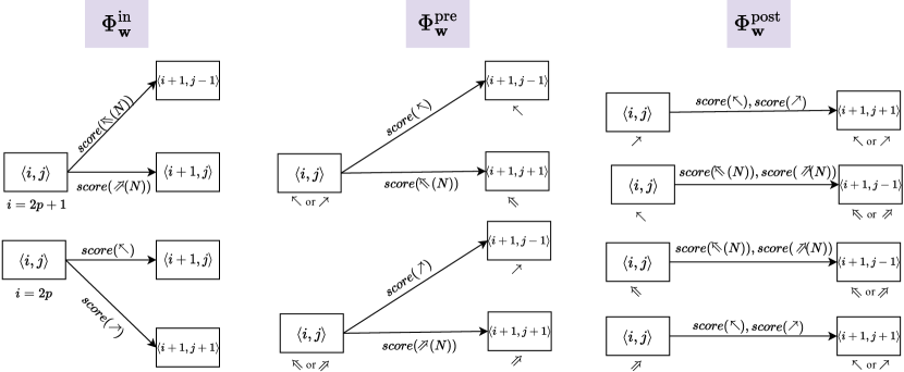
We start by introducing Kitaev and Klein’s (2020) dynamic program for their Φ𝐰insuperscriptsubscriptΦ𝐰in\color[rgb]{0,0,0}\definecolor[named]{pgfstrokecolor}{rgb}{0,0,0}\pgfsys@color@gray@stroke{0}\pgfsys@color@gray@fill{0}\Phi_{{\color[rgb]{0,0,0}\definecolor[named]{pgfstrokecolor}{rgb}{0,0,0}\pgfsys@color@gray@stroke{0}\pgfsys@color@gray@fill{0}\mathbf{w}}}^{\text{in}} model. Like many dynamic programs, theirs can be visualized as finding the highest-scoring path in a weighted directed acyclic graph (DAG). Each node in the DAG represents the number of generated tags i𝑖i and the current stack size j𝑗j. Each edge represents a transition weighted by the score of the associated tag predicted by the learner. Only sequences of exactly 2N12𝑁12N-1 tags will be valid. The odd tags must either be {\color[rgb]{0,0,0}\definecolor[named]{pgfstrokecolor}{rgb}{0,0,0}\pgfsys@color@gray@stroke{0}\pgfsys@color@gray@fill{0}\mathrel{\rotatebox[origin={c}]{45.0}{$\rightarrow$}}} or {\color[rgb]{0,0,0}\definecolor[named]{pgfstrokecolor}{rgb}{0,0,0}\pgfsys@color@gray@stroke{0}\pgfsys@color@gray@fill{0}\mathrel{\rotatebox[origin={c}]{135.0}{$\rightarrow$}}},666With the exception of the first tag that can only be {\color[rgb]{0,0,0}\definecolor[named]{pgfstrokecolor}{rgb}{0,0,0}\pgfsys@color@gray@stroke{0}\pgfsys@color@gray@fill{0}\mathrel{\rotatebox[origin={c}]{45.0}{$\rightarrow$}}}. and the even tags must be either {\color[rgb]{0,0,0}\definecolor[named]{pgfstrokecolor}{rgb}{0,0,0}\pgfsys@color@gray@stroke{0}\pgfsys@color@gray@fill{0}\mathrel{\rotatebox[origin={c}]{45.0}{$\Rightarrow$}}} or {\color[rgb]{0,0,0}\definecolor[named]{pgfstrokecolor}{rgb}{0,0,0}\pgfsys@color@gray@stroke{0}\pgfsys@color@gray@fill{0}\mathrel{\rotatebox[origin={c}]{135.0}{$\Rightarrow$}}}. The only accepted edges when generating the ithsuperscript𝑖thi^{\text{th}} tag (1<i2N11𝑖2𝑁11<i\leq 2N-1) in the sequence are shown in Fig. 2 left. The starting node is 1,111\langle 1,1\rangle, with {\color[rgb]{0,0,0}\definecolor[named]{pgfstrokecolor}{rgb}{0,0,0}\pgfsys@color@gray@stroke{0}\pgfsys@color@gray@fill{0}\mathrel{\rotatebox[origin={c}]{45.0}{$\rightarrow$}}} in the stack, and the goal is to reach the node: 2N1,12𝑁11\langle 2N-1,1\rangle.

Decoding Φ𝐰presuperscriptsubscriptΦ𝐰pre\color[rgb]{0,0,0}\definecolor[named]{pgfstrokecolor}{rgb}{0,0,0}\pgfsys@color@gray@stroke{0}\pgfsys@color@gray@fill{0}\Phi_{{\color[rgb]{0,0,0}\definecolor[named]{pgfstrokecolor}{rgb}{0,0,0}\pgfsys@color@gray@stroke{0}\pgfsys@color@gray@fill{0}\mathbf{w}}}^{\text{pre}} and Φ𝐰postsuperscriptsubscriptΦ𝐰post\color[rgb]{0,0,0}\definecolor[named]{pgfstrokecolor}{rgb}{0,0,0}\pgfsys@color@gray@stroke{0}\pgfsys@color@gray@fill{0}\Phi_{{\color[rgb]{0,0,0}\definecolor[named]{pgfstrokecolor}{rgb}{0,0,0}\pgfsys@color@gray@stroke{0}\pgfsys@color@gray@fill{0}\mathbf{w}}}^{\text{post}}.

To adapt the algorithm introduced above to work with pre-order linearization, we first investigate what makes a pre-order tagging sequence valid:

  • When a reduce tag ({\color[rgb]{0,0,0}\definecolor[named]{pgfstrokecolor}{rgb}{0,0,0}\pgfsys@color@gray@stroke{0}\pgfsys@color@gray@fill{0}\mathrel{\rotatebox[origin={c}]{45.0}{$\Rightarrow$}}} or {\color[rgb]{0,0,0}\definecolor[named]{pgfstrokecolor}{rgb}{0,0,0}\pgfsys@color@gray@stroke{0}\pgfsys@color@gray@fill{0}\mathrel{\rotatebox[origin={c}]{135.0}{$\Rightarrow$}}}) is generated, there must be at least one node in the stack, and after performing the reduce, the size of the stack is increased by one.

  • Immediately after shifting a node, we either process (perform a shift or reduce on) that node’s right sibling or shift the right sibling. Therefore, the only valid tags to generate subsequently are {\color[rgb]{0,0,0}\definecolor[named]{pgfstrokecolor}{rgb}{0,0,0}\pgfsys@color@gray@stroke{0}\pgfsys@color@gray@fill{0}\mathrel{\rotatebox[origin={c}]{135.0}{$\rightarrow$}}} or {\color[rgb]{0,0,0}\definecolor[named]{pgfstrokecolor}{rgb}{0,0,0}\pgfsys@color@gray@stroke{0}\pgfsys@color@gray@fill{0}\mathrel{\rotatebox[origin={c}]{135.0}{$\Rightarrow$}}}.

  • Immediately after reducing a node, we process (perform a shift or reduce on) its left child. Therefore, it is only valid to generate either {\color[rgb]{0,0,0}\definecolor[named]{pgfstrokecolor}{rgb}{0,0,0}\pgfsys@color@gray@stroke{0}\pgfsys@color@gray@fill{0}\mathrel{\rotatebox[origin={c}]{45.0}{$\rightarrow$}}} or {\color[rgb]{0,0,0}\definecolor[named]{pgfstrokecolor}{rgb}{0,0,0}\pgfsys@color@gray@stroke{0}\pgfsys@color@gray@fill{0}\mathrel{\rotatebox[origin={c}]{45.0}{$\Rightarrow$}}}.

The above constraints suggest that if we know the previous tag type (shift or reduce) and the stack size at each step of generation, we can form the valid transitions from each node $\langle i,j\rangle$. Such transitions are shown in Fig. 2 center. Similarly, the valid transitions for decoding post-order linearization are shown in the right part of Fig. 2.

Time Complexity.

The complexity of the dynamic program to find the highest-scoring path depends on the number of unique tags 𝒪(|𝒩|)𝒪𝒩\mathcal{O}\!\left(|{\color[rgb]{0,0,0}\definecolor[named]{pgfstrokecolor}{rgb}{0,0,0}\pgfsys@color@gray@stroke{0}\pgfsys@color@gray@fill{0}\mathcal{N}}|\right), the length of the tag sequence $\mathcal{O}\!\left(N\right)$, and the stack size $d$. Linearization schemes derived from the right-corner transform tend to have smaller stack sizes (Abney and Johnson, 1991; Schuler et al., 2010).777For purely left- or right-branching trees, the left-corner or right-corner transformations, respectively, provably reduce the stack size to one (Johnson, 1998). These transformations could increase the stack size for centered-embedded trees. However, such trees are rare in natural language as they are difficult for humans to comprehend (Gibson, 1998). As a result, one can often derive a faster, exact decoding algorithm for such schemes. Please refer to App. C for a more formal treatment of the dynamic program for finding the highest-scoring tag sequence using these transitions (Algorithm 1).

An 𝒪(dN|𝒩|2)𝒪𝑑𝑁superscript𝒩2\mathcal{O}\!\left(dN|{\color[rgb]{0,0,0}\definecolor[named]{pgfstrokecolor}{rgb}{0,0,0}\pgfsys@color@gray@stroke{0}\pgfsys@color@gray@fill{0}\mathcal{N}}|^{2}\right) Algorithm.

As discussed in § 4, one can break the independence assumption in Eq. 2 by making each tag dependent on the previously generated tag. Consequently, when finding the highest-scoring path in the decoding step, we should remember the last generated tag. Therefore, in addition to $i$ and $j$, the generated tag must be stored. This adds 𝒪(|𝒩|)𝒪𝒩\mathcal{O}\!\left(|{\color[rgb]{0,0,0}\definecolor[named]{pgfstrokecolor}{rgb}{0,0,0}\pgfsys@color@gray@stroke{0}\pgfsys@color@gray@fill{0}\mathcal{N}}|\right) extra memory per node, and increases the runtime complexity to 𝒪(dN|𝒩|2)𝒪𝑑𝑁superscript𝒩2\mathcal{O}\!\left(dN|{\color[rgb]{0,0,0}\definecolor[named]{pgfstrokecolor}{rgb}{0,0,0}\pgfsys@color@gray@stroke{0}\pgfsys@color@gray@fill{0}\mathcal{N}}|^{2}\right). Please refer to App. C for a more formal treatment of the dynamic program for finding the highest-scoring tag sequence (Algorithm 2).

5.2 Beam Search Decoding

We can speed up the dynamic programming algorithms above if we forego the desire for an exact algorithm. In such a case, applying beam search presents a reasonable alternative where we only keep track of $h$ tag sequences with the highest score at each step of the tag generation. Although no longer an exact algorithm, beam search reduces the time complexity to 𝒪(hloghN|𝒩|)𝒪𝑁𝒩\mathcal{O}\!\left(h\log h\,N|{\color[rgb]{0,0,0}\definecolor[named]{pgfstrokecolor}{rgb}{0,0,0}\pgfsys@color@gray@stroke{0}\pgfsys@color@gray@fill{0}\mathcal{N}}|\right).888This can be improved to 𝒪(hN|𝒩|)𝒪𝑁𝒩\mathcal{O}\!\left(hN|{\color[rgb]{0,0,0}\definecolor[named]{pgfstrokecolor}{rgb}{0,0,0}\pgfsys@color@gray@stroke{0}\pgfsys@color@gray@fill{0}\mathcal{N}}|\right) with quick select. This can result in a substantial speed-up over the dynamic programs presented above when $d$, the maximum required stack size, is much larger than the beam size $h$. We empirically measure the trade-off between accuracy and speed in our experiments.

Basque French German Hebrew Hungarian Korean Polish Swedish
Kitaev et al. (2019) 91.63 87.42 90.20 92.99 94.90 88.80 96.36 88.86
Kitaev and Klein (2018) 89.71 84.06 87.69 90.35 92.69 86.59 93.69 84.45
in-order-[indep.] 89.86 84.54 88.34 91.40 93.81 84.89 95.20 86.66
pre-order-[indep.] 87.98 84.76 88.18 89.45 90.69 81.81 94.84 84.65
post-order-[indep.] 81.05 56.97 78.07 64.21 76.24 86.64 86.91 58.44
Table 2: Comparison of FMeasure of different tagging schemata on the SPMRL test set

6 Experiments

In our experimental section we aim to answer two questions: (i) What is the effect of each design decision on the efficiency and accuracy of a tagger, and which design decisions have the greatest effect? (ii) Are the best design choices consistent across languages?

Data.

We use two data sources: the Penn Treebank (Marcus et al., 1993) for English constituency parsing and Statistical Parsing of Morphologically Rich Languages (SPMRL) 2013/2014 shared tasks (Seddah et al., 2013, 2014) for 8 languages: Basque, French, German, Hebrew, Hungarian, Korean, Polish, and Swedish. We provide the dataset statistics in Table 5. We perform similar preprocessing as Kitaev and Klein (2020), which we explain in App. F. For evaluation, the evalb Perl script999http://nlp.cs.nyu.edu/evalb/ is used to calculate FMeasure of the parse tree. We use only one GPU node for the reported inference times. Further experimental details can be found in App. G.

6.1 What Makes a Good Tagger?

Linearization.

First, we measure the effect of linearization and alignment on the performance of the parser. We train BERT101010We use bert-large-uncased from the Huggingface library (Wolf et al., 2020). on the English dataset. While keeping the learning schema fixed, we experiment with three linearizations: Φ𝐰insuperscriptsubscriptΦ𝐰in\color[rgb]{0,0,0}\definecolor[named]{pgfstrokecolor}{rgb}{0,0,0}\pgfsys@color@gray@stroke{0}\pgfsys@color@gray@fill{0}\Phi_{{\color[rgb]{0,0,0}\definecolor[named]{pgfstrokecolor}{rgb}{0,0,0}\pgfsys@color@gray@stroke{0}\pgfsys@color@gray@fill{0}\mathbf{w}}}^{\text{in}}, Φ𝐰postsuperscriptsubscriptΦ𝐰post\color[rgb]{0,0,0}\definecolor[named]{pgfstrokecolor}{rgb}{0,0,0}\pgfsys@color@gray@stroke{0}\pgfsys@color@gray@fill{0}\Phi_{{\color[rgb]{0,0,0}\definecolor[named]{pgfstrokecolor}{rgb}{0,0,0}\pgfsys@color@gray@stroke{0}\pgfsys@color@gray@fill{0}\mathbf{w}}}^{\text{post}}, and Φ𝐰presuperscriptsubscriptΦ𝐰pre\color[rgb]{0,0,0}\definecolor[named]{pgfstrokecolor}{rgb}{0,0,0}\pgfsys@color@gray@stroke{0}\pgfsys@color@gray@fill{0}\Phi_{{\color[rgb]{0,0,0}\definecolor[named]{pgfstrokecolor}{rgb}{0,0,0}\pgfsys@color@gray@stroke{0}\pgfsys@color@gray@fill{0}\mathbf{w}}}^{\text{pre}}. We observe that the in-order shift–reduce linearizer leads to the best FMeasure ($95.15$), followed by the top-down linearizer ($94.56$). There is a considerable gap between the performance of a tagger with the post-order linearizer ($89.23$) and other taggers, as shown in Table 3. The only difference between these taggers is the linearization function, and more specifically, the deviation between tags and the input sequence as defined in Def. 4. This result suggests that deviation is an important factor in designing accurate taggers.

Learning Schema.

Second, we measure the effect of the independence assumption in scoring tagging sequences. We slightly change the scoring mechanism by training a CRF111111We use our custom implementation of CRF with pytorch. and an LSTM layer121212We use a two-layered biLSTM network, with the hidden size equal to the tags vocabulary size $|\mathcal{T}|$ (approximately 150 cells). For further details please refer to App. G. to make scoring over tags left- or right-dependent. We expect to see improvements with Φ𝐰presuperscriptsubscriptΦ𝐰pre\color[rgb]{0,0,0}\definecolor[named]{pgfstrokecolor}{rgb}{0,0,0}\pgfsys@color@gray@stroke{0}\pgfsys@color@gray@fill{0}\Phi_{{\color[rgb]{0,0,0}\definecolor[named]{pgfstrokecolor}{rgb}{0,0,0}\pgfsys@color@gray@stroke{0}\pgfsys@color@gray@fill{0}\mathbf{w}}}^{\text{pre}} and Φ𝐰postsuperscriptsubscriptΦ𝐰post\color[rgb]{0,0,0}\definecolor[named]{pgfstrokecolor}{rgb}{0,0,0}\pgfsys@color@gray@stroke{0}\pgfsys@color@gray@fill{0}\Phi_{{\color[rgb]{0,0,0}\definecolor[named]{pgfstrokecolor}{rgb}{0,0,0}\pgfsys@color@gray@stroke{0}\pgfsys@color@gray@fill{0}\mathbf{w}}}^{\text{post}}, since in these two cases, creating such dependencies gives us more expressive power in terms of the distributions over trees that can be modeled. However, we only observe marginal improvements when we add left and right dependencies (see Table 3). Thus, we hypothesize that BERT already captures the dependencies between the words.

Beam Search DP
FMeasure Sents/s FMeasure Sents/s
in-order [indep.] 91.59 156 95.15 128
pre-order [indep.] 93.57 114 94.56 51
pre-order [left dep. crf] 93.65 110 94.47 21
pre-order [left dep. lstm] 93.78 110 94.38 20
post-order [indep.] 85.38 108 89.23 29
post-order [right dep. crf] 82.28 108 88.28 5
post-order [right dep. lstm] 85.25 103 89.61 5
Table 3: Comparison of parsing metrics on the WSJ test set. This is the exact equivalent setup to tetratagger. However, because we neither use the exact same code nor the hardware, the numbers do not exactly match with what is reported in the original paper.

Decoding Schema.

Third, we assess the trade-off between accuracy and efficiency caused by using beam search versus exact decoding. We take $h=10$ as the beam size. As shown in Table 3, taggers with post-order linearization take longer to decode using the exact dynamic program. This is largely due to the fact that they need deeper stacks in the decoding process (see App. E for a comparison). In such scenarios, we see that beam search leads to a significant speed-up in decoding time, at the expense of a drop (between 3 to 6 points) in FMeasure. However, the drop in accuracy observed with the pre-order linearization is less than 1 point. Therefore, in some cases, beam search may be able to offer a sweet spot between speed and accuracy. To put these results into context, we see taggers with in-order and pre-order linearizations achieve comparable results to state-of-the-art parsers with custom architectures, where the state-of-the-art parser achieves 95.84 FMeasure (Zhou and Zhao, 2019).

6.2 Multilingual Parsing

As shown in the previous experiment, linearization plays an important role in constructing an accurate tagger. Moreover, we observe that in-order linearizers yield the best-performing taggers, followed by the pre-order and post-order linearizers. In our second set of experiments, we attempt to replicate this result in languages other than English. We train BERT-based learners131313We use bert-base-multilingual-cased. on 8 additional typologically diverse languages. As the results in Table 2 suggest, in general, taggers can achieve competitive FMeasures relative to parsers with custom architectures (Kitaev and Klein, 2018).

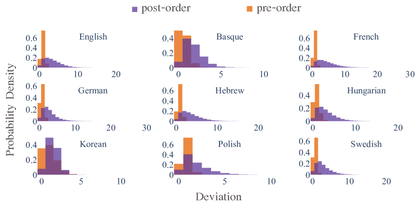
Similar to results in English, in most of the other eight languages, taggers with in-order linearizers achieve the best FMeasure. We note that the gap between the performance of post and pre-order linearization varies significantly across languages. To further investigate this finding, we compute the distribution of deviation in alignment at the word level (based on Def. 4). For most languages, the deviation of the pre-order linearizer peaks close to zero. On the contrary, in French, Swedish, and Hebrew, the post-order linearizers do not align very well with the input sequence. Indeed, we observe derivations of up to 30 for some words in these languages. This is not surprising because these languages tend to be right-branching. In fact, we observe a large gap between the performance of taggers with pre- and post-order linearizers in these three languages.

On the other hand, for a left-branching language like Korean, post-order linearization aligns nicely with the input sequence. This is also very well reflected in the parsing results, where the tagger with post-order linearization performs better than taggers using in-order or pre-order linearization.

Our findings suggest that a tagger’s performance depends on the deviation of its linearizer. We measure this via Pearson’s correlation between parsers’ FMeasure and the mean deviation of the linearizer, per language. We see that the two variables are negatively correlated ($-0.77$) with a $p$ value of $0.0001$.We conclude that the deviation in the alignment of tags with the input sequence is highly dependent on the characteristics of the language.

7 Conclusion

In this paper, we analyze parsing as tagging, a relatively new paradigm for developing statistical parsers of natural language. We show many parsing-as-tagging schemes are actually closely related to the well-studied shift–-reduce parsers. We also show that Kitaev and Klein’s (2020) tetratagging scheme is, in fact, an in-order shift–reduce parser, which can be derived from bottom-up or top-down shift–reduce parsing on the right or left-cornered grammars, respectively. We further identify three common steps in parsing-as-tagging pipelines and explore various design decisions at each step. Empirically, we evaluate the effect of such design decisions on the speed and accuracy of the resulting parser. Our results suggest that there is a strong negative correlation between the deviation metric and the accuracy of constituency parsers.

Ethical Concerns

We do not believe the work presented here further amplifies biases already present in the datasets and the algorithms that we experiment with because our work is primarily a theoretical analysis of existing work. Therefore, we foresee no ethical concerns in this work.

Limitations

This work only focuses on constituency parsing. Therefore, the results might not fully generalize to other parsing tasks, e.g., dependency parsing. Furthermore, in our experiments, we only focus on comparing design decisions of parsing-as-tagging schemes, and not on achieving state-of-the-art results. We believe that by using larger pre-trained models, one might be able to obtain better parsing performance with the tagging pipelines discussed in this paper. In addition, in our multilingual analysis, the only left-branching language that we had access to was Korean, therefore, more analysis needs to be done on left-branching languages.

Acknowledgments

We would like to thank Nikita Kitaev, Tim Vieira, Carlos Gómez-Rodríguez, and Jason Eisner for fruitful discussions on a preliminary draft of the paper. We would also like to thank anonymous reviewers for their insightful feedback during the review process. We also thank Zeerak Talat and Clément Guerner for their feedback on this manuscript. Afra Amini is supported by ETH AI Center doctoral fellowship.

References

  • Abney and Johnson (1991) Steven P. Abney and Mark Johnson. 1991. Memory requirements and local ambiguities of parsing strategies. Journal of Psycholinguistic Research, 20(3):233–250.
  • Aho and Ullman (1972) Alfred V. Aho and Jeffrey D. Ullman. 1972. The Theory of Parsing, Translation and Compiling, volume 1. Prentice-Hall, Englewood Cliffs, NJ.
  • Butoi et al. (2022) Alexandra Butoi, Brian DuSell, Tim Vieira, Ryan Cotterell, and David Chiang. 2022. Algorithms for weighted pushdown automata. In Proceedings of the 2022 Conference on Empirical Methods in Natural Language Processing. Association for Computational Linguistics.
  • Devlin et al. (2019) Jacob Devlin, Ming-Wei Chang, Kenton Lee, and Kristina Toutanova. 2019. BERT: Pre-training of deep bidirectional transformers for language understanding. In Proceedings of the 2019 Conference of the North American Chapter of the Association for Computational Linguistics: Human Language Technologies, Volume 1 (Long and Short Papers), pages 4171–4186, Minneapolis, Minnesota. Association for Computational Linguistics.
  • Fraser (1989) Norman Fraser. 1989. Parsing and dependency grammar. In UCL Working Papers in Linguistics 1: University College London., pages 296–319.
  • Gibson (1998) Edward Gibson. 1998. Linguistic complexity: locality of syntactic dependencies. Cognition, 68(1):1–76.
  • Gómez-Rodríguez et al. (2020) Carlos Gómez-Rodríguez, Michalina Strzyz, and David Vilares. 2020. A unifying theory of transition-based and sequence labeling parsing. In Proceedings of the 28th International Conference on Computational Linguistics, pages 3776–3793, Barcelona, Spain (Online). International Committee on Computational Linguistics.
  • Gómez-Rodríguez and Vilares (2018) Carlos Gómez-Rodríguez and David Vilares. 2018. Constituent parsing as sequence labeling. In Proceedings of the 2018 Conference on Empirical Methods in Natural Language Processing, pages 1314–1324, Brussels, Belgium. Association for Computational Linguistics.
  • Hochreiter and Schmidhuber (1997) Sepp Hochreiter and Jürgen Schmidhuber. 1997. Long Short-Term Memory. Neural Computation, 9(8):1735–1780.
  • Johnson (1998) Mark Johnson. 1998. Finite-state approximation of constraint-based grammars using left-corner grammar transforms. In 36th Annual Meeting of the Association for Computational Linguistics and 17th International Conference on Computational Linguistics, Volume 1, pages 619–623, Montreal, Quebec, Canada. Association for Computational Linguistics.
  • Kiperwasser and Ballesteros (2018) Eliyahu Kiperwasser and Miguel Ballesteros. 2018. Scheduled multi-task learning: From syntax to translation. Transactions of the Association for Computational Linguistics, 6:225–240.
  • Kitaev et al. (2019) Nikita Kitaev, Steven Cao, and Dan Klein. 2019. Multilingual constituency parsing with self-attention and pre-training. In Proceedings of the 57th Annual Meeting of the Association for Computational Linguistics, pages 3499–3505, Florence, Italy. Association for Computational Linguistics.
  • Kitaev and Klein (2018) Nikita Kitaev and Dan Klein. 2018. Constituency parsing with a self-attentive encoder. In Proceedings of the 56th Annual Meeting of the Association for Computational Linguistics (Volume 1: Long Papers), pages 2676–2686, Melbourne, Australia. Association for Computational Linguistics.
  • Kitaev and Klein (2020) Nikita Kitaev and Dan Klein. 2020. Tetra-tagging: Word-synchronous parsing with linear-time inference. In Proceedings of the 58th Annual Meeting of the Association for Computational Linguistics, pages 6255–6261, Online. Association for Computational Linguistics.
  • Lafferty et al. (2001) John D. Lafferty, Andrew McCallum, and Fernando C. N. Pereira. 2001. Conditional random fields: Probabilistic models for segmenting and labeling sequence data. In Proceedings of the Eighteenth International Conference on Machine Learning, ICML ’01, page 282–289, San Francisco, CA, USA. Morgan Kaufmann Publishers Inc.
  • Lang (1974) Bernard Lang. 1974. Deterministic techniques for efficient non-deterministic parsers. In Automata, Languages and Programming, pages 255–269, Berlin, Heidelberg. Springer Berlin Heidelberg.
  • Li et al. (2018) Zuchao Li, Jiaxun Cai, Shexia He, and Hai Zhao. 2018. Seq2seq dependency parsing. In Proceedings of the 27th International Conference on Computational Linguistics, pages 3203–3214, Santa Fe, New Mexico, USA. Association for Computational Linguistics.
  • Liu and Zhang (2017) Jiangming Liu and Yue Zhang. 2017. In-order transition-based constituent parsing. Transactions of the Association for Computational Linguistics, 5:413–424.
  • Marcus et al. (1993) Mitchell P. Marcus, Beatrice Santorini, and Mary Ann Marcinkiewicz. 1993. Building a large annotated corpus of English: The Penn Treebank. Computational Linguistics, 19(2):313–330.
  • Nivre (2004) Joakim Nivre. 2004. Incrementality in deterministic dependency parsing. In Proceedings of the Workshop on Incremental Parsing: Bringing Engineering and Cognition Together, pages 50–57, Barcelona, Spain. Association for Computational Linguistics.
  • Nivre (2008) Joakim Nivre. 2008. Algorithms for deterministic incremental dependency parsing. Computational Linguistics, 34(4):513–553.
  • Sagae and Lavie (2005) Kenji Sagae and Alon Lavie. 2005. A classifier-based parser with linear run-time complexity. In Proceedings of the Ninth International Workshop on Parsing Technology, pages 125–132, Vancouver, British Columbia. Association for Computational Linguistics.
  • Schuler et al. (2010) William Schuler, Samir AbdelRahman, Tim Miller, and Lane Schwartz. 2010. Broad-coverage parsing using human-like memory constraints. Computational Linguistics, 36(1):1–30.
  • Seddah et al. (2014) Djamé Seddah, Sandra Kübler, and Reut Tsarfaty. 2014. Introducing the SPMRL 2014 shared task on parsing morphologically-rich languages. In Proceedings of the First Joint Workshop on Statistical Parsing of Morphologically Rich Languages and Syntactic Analysis of Non-Canonical Languages, pages 103–109, Dublin, Ireland. Dublin City University.
  • Seddah et al. (2013) Djamé Seddah, Reut Tsarfaty, Sandra Kübler, Marie Candito, Jinho D. Choi, Richárd Farkas, Jennifer Foster, Iakes Goenaga, Koldo Gojenola Galletebeitia, Yoav Goldberg, Spence Green, Nizar Habash, Marco Kuhlmann, Wolfgang Maier, Joakim Nivre, Adam Przepiórkowski, Ryan Roth, Wolfgang Seeker, Yannick Versley, Veronika Vincze, Marcin Woliński, Alina Wróblewska, and Eric Villemonte de la Clergerie. 2013. Overview of the SPMRL 2013 shared task: A cross-framework evaluation of parsing morphologically rich languages. In Proceedings of the Fourth Workshop on Statistical Parsing of Morphologically-Rich Languages, pages 146–182, Seattle, Washington, USA. Association for Computational Linguistics.
  • Strzyz (2021) Michalina Strzyz. 2021. Viability of Sequence Labeling Encodings for Dependency Parsing. Ph.D. thesis, University of A Coruña.
  • Strzyz et al. (2019) Michalina Strzyz, David Vilares, and Carlos Gómez-Rodríguez. 2019. Viable dependency parsing as sequence labeling. In Proceedings of the 2019 Conference of the North American Chapter of the Association for Computational Linguistics: Human Language Technologies, Volume 1 (Long and Short Papers), pages 717–723, Minneapolis, Minnesota. Association for Computational Linguistics.
  • Vacareanu et al. (2020) Robert Vacareanu, George Caique Gouveia Barbosa, Marco A. Valenzuela-Escárcega, and Mihai Surdeanu. 2020. Parsing as tagging. In Proceedings of the 12th Language Resources and Evaluation Conference, pages 5225–5231, Marseille, France. European Language Resources Association.
  • Vilares et al. (2019) David Vilares, Mostafa Abdou, and Anders Søgaard. 2019. Better, faster, stronger sequence tagging constituent parsers. In Proceedings of the 2019 Conference of the North American Chapter of the Association for Computational Linguistics: Human Language Technologies, Volume 1 (Long and Short Papers), pages 3372–3383, Minneapolis, Minnesota. Association for Computational Linguistics.
  • Wolf et al. (2020) Thomas Wolf, Lysandre Debut, Victor Sanh, Julien Chaumond, Clement Delangue, Anthony Moi, Pierric Cistac, Tim Rault, Rémi Louf, Morgan Funtowicz, Joe Davison, Sam Shleifer, Patrick von Platen, Clara Ma, Yacine Jernite, Julien Plu, Canwen Xu, Teven Le Scao, Sylvain Gugger, Mariama Drame, Quentin Lhoest, and Alexander M. Rush. 2020. Transformers: State-of-the-art natural language processing. In Proceedings of the 2020 Conference on Empirical Methods in Natural Language Processing: System Demonstrations, pages 38–45, Online. Association for Computational Linguistics.
  • Xu et al. (2014) Wenduan Xu, Stephen Clark, and Yue Zhang. 2014. Shift-reduce CCG parsing with a dependency model. In Proceedings of the 52nd Annual Meeting of the Association for Computational Linguistics (Volume 1: Long Papers), pages 218–227, Baltimore, Maryland. Association for Computational Linguistics.
  • Yamada and Matsumoto (2003) Hiroyasu Yamada and Yuji Matsumoto. 2003. Statistical dependency analysis with support vector machines. In Proceedings of the Eighth International Conference on Parsing Technologies, pages 195–206, Nancy, France.
  • Zhang and Clark (2009) Yue Zhang and Stephen Clark. 2009. Transition-based parsing of the Chinese treebank using a global discriminative model. In Proceedings of the 11th International Conference on Parsing Technologies (IWPT’09), pages 162–171, Paris, France. Association for Computational Linguistics.
  • Zhang and Clark (2011) Yue Zhang and Stephen Clark. 2011. Shift-reduce CCG parsing. In Proceedings of the 49th Annual Meeting of the Association for Computational Linguistics: Human Language Technologies, pages 683–692, Portland, Oregon, USA. Association for Computational Linguistics.
  • Zhou and Zhao (2019) Junru Zhou and Hai Zhao. 2019. Head-driven phrase structure grammar parsing on Penn Treebank. In Proceedings of the 57th Annual Meeting of the Association for Computational Linguistics, pages 2396–2408, Florence, Italy. Association for Computational Linguistics.
  • Zhu et al. (2013) Muhua Zhu, Yue Zhang, Wenliang Chen, Min Zhang, and Jingbo Zhu. 2013. Fast and accurate shift-reduce constituent parsing. In Proceedings of the 51st Annual Meeting of the Association for Computational Linguistics (Volume 1: Long Papers), pages 434–443, Sofia, Bulgaria. Association for Computational Linguistics.

Appendix A Related Work

We provide a comparative review of parsing as tagging works on both dependency and constituency parsing, focusing on their design decisions at different steps of the pipeline.

A.1 Dependency Parsing as Tagging

Previous work on dependency parsing as tagging linearizes the dependency tree by iterating through the dependency arcs and encoding the relative position of the child with respect to its parent in the tag sequence (Li et al., 2018; Kiperwasser and Ballesteros, 2018). Each word is then aligned with the tag indicating its relative position with respect to its head. At the decoding step, to prevent the model from generating dependency arcs that do not form valid dependency trees, a tree constraint is often applied (Li et al., 2018). Similarly, Vacareanu et al. (2020) employ contextualized embeddings of the input with the same tagging schema. Strzyz et al. (2019) provide a framework and train and compare various dependency parsers as taggers. See also Strzyz (2021) for further comparison.

Closest to our work, Gómez-Rodríguez et al. (2020) suggest a linearization and alignment scheme that works with any transition-based parser to create a sequence of tags from a sequence of actions. Therefore, their method applies to both constituency and dependency parsing. For instance, turning a shift–reduce parser into a tag sequence requires creating a tag for all the reduce actions up to each shift action. While this construction results in exactly $N$ tags, there are in general an exponentially large number of tags. To compare this approach with the linearizations discussed in this paper, we must note that while such a schema is shift-aligned, it might not evenly align the tags with the input sequence. Moreover, the in-order linearization scheme discussed here has a small number of tags.

A.2 Constituency Parsing as Tagging

Gómez-Rodríguez and Vilares (2018) provide an in-order linearization of the derivation tree, where they encode nonterminals and their depth as a tagging sequence. Since the depth is encoded in the tags themselves, the tag set size is unbounded and is dependent on the input. Kitaev and Klein (2020) improve upon Gómez-Rodríguez and Vilares’s (2018) encoding by discovering a similar tagging system that has only four tags. In Kitaev and Klein’s (2020) linearization step, they encode both terminals and nonterminals in the tag sequence, as well as the direction of a node with respect to its parent. Using a pretrained BERT model to score tags, they show that their approach reaches state-of-the-art performance despite being architecturally simpler. Furthermore, the parser is significantly faster than competing approaches.

d𝐰subscript𝑑𝐰{\color[rgb]{0,0,0}\definecolor[named]{pgfstrokecolor}{rgb}{0,0,0}\pgfsys@color@gray@stroke{0}\pgfsys@color@gray@fill{0}d_{{\color[rgb]{0,0,0}\definecolor[named]{pgfstrokecolor}{rgb}{0,0,0}\pgfsys@color@gray@stroke{0}\pgfsys@color@gray@fill{0}\mathbf{w}}}} {forest} for tree=myleaf/.style=label=[align=center]below:#1 [$\mathrm{N}$[$\mathrm{N}_{1}$[$\mathrm{X}_{i}$, myleaf=$w_{i}$, circle, draw, fill=lightgray][,phantom]][,phantom]] {forest} for tree=myleaf/.style=label=[align=center]below:#1 [$\mathrm{N}$[,phantom][$\mathrm{N}_{1}$ [$\mathrm{X}_{i}$, myleaf=$w_{i}$, circle, draw, fill=lightgray][,phantom]]] {forest} for tree=myleaf/.style=label=[align=center]below:#1 [[$\mathrm{N}$ [$\mathrm{N}_{1}$ [,phantom] [$\mathrm{X}_{i}$, myleaf=$w_{i}$, circle, draw, fill=lightgray]] [,phantom]][,phantom]] {forest} for tree=myleaf/.style=label=[align=center]below:#1 [[,phantom][$\mathrm{N}$ [$\mathrm{N}_{1}$ [,phantom] [$\mathrm{X}_{i}$, myleaf=$w_{i}$, circle, draw, fill=lightgray]] [,phantom]]] {forest} for tree=myleaf/.style=label=[align=center]below:#1 [$\mathrm{S}$ [,phantom] […[,phantom] [$\mathrm{N}_{1}$ [,phantom] [$\mathrm{X}_{i}$, myleaf=$w_{i}$, circle, draw, fill=lightgray]]]]
Φ𝐰insuperscriptsubscriptΦ𝐰in\color[rgb]{0,0,0}\definecolor[named]{pgfstrokecolor}{rgb}{0,0,0}\pgfsys@color@gray@stroke{0}\pgfsys@color@gray@fill{0}\Phi_{{\color[rgb]{0,0,0}\definecolor[named]{pgfstrokecolor}{rgb}{0,0,0}\pgfsys@color@gray@stroke{0}\pgfsys@color@gray@fill{0}\mathbf{w}}}^{\text{in}} (N1){\color[rgb]{0,0,0}\definecolor[named]{pgfstrokecolor}{rgb}{0,0,0}\pgfsys@color@gray@stroke{0}\pgfsys@color@gray@fill{0}\mathrel{\rotatebox[origin={c}]{45.0}{$\rightarrow$}}}{\color[rgb]{0,0,0}\definecolor[named]{pgfstrokecolor}{rgb}{0,0,0}\pgfsys@color@gray@stroke{0}\pgfsys@color@gray@fill{0}\mathrel{\rotatebox[origin={c}]{45.0}{$\Rightarrow$}}}{\scriptstyle(\mathrm{N}_{1})} (N1){\color[rgb]{0,0,0}\definecolor[named]{pgfstrokecolor}{rgb}{0,0,0}\pgfsys@color@gray@stroke{0}\pgfsys@color@gray@fill{0}\mathrel{\rotatebox[origin={c}]{45.0}{$\rightarrow$}}}{\color[rgb]{0,0,0}\definecolor[named]{pgfstrokecolor}{rgb}{0,0,0}\pgfsys@color@gray@stroke{0}\pgfsys@color@gray@fill{0}\mathrel{\rotatebox[origin={c}]{135.0}{$\Rightarrow$}}}{\scriptstyle(\mathrm{N}_{1})} (N){\color[rgb]{0,0,0}\definecolor[named]{pgfstrokecolor}{rgb}{0,0,0}\pgfsys@color@gray@stroke{0}\pgfsys@color@gray@fill{0}\mathrel{\rotatebox[origin={c}]{135.0}{$\rightarrow$}}}{\color[rgb]{0,0,0}\definecolor[named]{pgfstrokecolor}{rgb}{0,0,0}\pgfsys@color@gray@stroke{0}\pgfsys@color@gray@fill{0}\mathrel{\rotatebox[origin={c}]{45.0}{$\Rightarrow$}}}{\scriptstyle(\mathrm{N})} (N){\color[rgb]{0,0,0}\definecolor[named]{pgfstrokecolor}{rgb}{0,0,0}\pgfsys@color@gray@stroke{0}\pgfsys@color@gray@fill{0}\mathrel{\rotatebox[origin={c}]{135.0}{$\rightarrow$}}}{\color[rgb]{0,0,0}\definecolor[named]{pgfstrokecolor}{rgb}{0,0,0}\pgfsys@color@gray@stroke{0}\pgfsys@color@gray@fill{0}\mathrel{\rotatebox[origin={c}]{135.0}{$\Rightarrow$}}}{\scriptstyle(\mathrm{N})} {\color[rgb]{0,0,0}\definecolor[named]{pgfstrokecolor}{rgb}{0,0,0}\pgfsys@color@gray@stroke{0}\pgfsys@color@gray@fill{0}\mathrel{\rotatebox[origin={c}]{135.0}{$\rightarrow$}}}
d𝐰rcsuperscriptsubscript𝑑𝐰rc\color[rgb]{0,0,0}\definecolor[named]{pgfstrokecolor}{rgb}{0,0,0}\pgfsys@color@gray@stroke{0}\pgfsys@color@gray@fill{0}{d_{{\color[rgb]{0,0,0}\definecolor[named]{pgfstrokecolor}{rgb}{0,0,0}\pgfsys@color@gray@stroke{0}\pgfsys@color@gray@fill{0}\mathbf{w}}}^{\text{rc}}} {forest} for tree=myleaf/.style=label=[align=center]below:#1 [$\mathrm{N}_{1}/.$[$\mathrm{N}_{1}/.$[$\varepsilon$][$\mathrm{X}_{i}$, myleaf=$w_{i}$, circle, draw, fill=lightgray]][,phantom]] {forest} for tree=myleaf/.style=label=[align=center]below:#1 [$\mathrm{N}^{\prime}$[$\mathrm{N}^{\prime}/.$ [$\mathrm{N}^{\prime}/\mathrm{N}_{1}$] [$\mathrm{X}_{i}$, myleaf=$w_{i}$, circle, draw, fill=lightgray]][,phantom]] {forest} for tree=myleaf/.style=label=[align=center]below:#1 [[$\mathrm{N}/.$ [$\varepsilon$][$\mathrm{N}_{1}$ [$\mathrm{N}_{1}/.$] [$\mathrm{X}_{i}$, myleaf=$w_{i}$, circle, draw, fill=lightgray]]][,phantom]] {forest} for tree=myleaf/.style=label=[align=center]below:#1 [[$\mathrm{N}^{\prime}/.$ [$\mathrm{N}^{\prime}/\mathrm{N}$][$\mathrm{N}_{1}$ [$\mathrm{N}_{1}/.$] [$\mathrm{X}_{i}$, myleaf=$w_{i}$, circle, draw, fill=lightgray]]][,phantom]] {forest} for tree=myleaf/.style=label=[align=center]below:#1 [$\mathrm{S}$ [$\mathrm{S}/.$] [$\mathrm{X}_{i}$, myleaf=$w_{i}$, circle, draw, fill=lightgray]]]
Φ𝐰postsuperscriptsubscriptΦ𝐰post\color[rgb]{0,0,0}\definecolor[named]{pgfstrokecolor}{rgb}{0,0,0}\pgfsys@color@gray@stroke{0}\pgfsys@color@gray@fill{0}\Phi_{{\color[rgb]{0,0,0}\definecolor[named]{pgfstrokecolor}{rgb}{0,0,0}\pgfsys@color@gray@stroke{0}\pgfsys@color@gray@fill{0}\mathbf{w}}}^{\text{post}} {\scriptstyle{\color[rgb]{0,0,0}\definecolor[named]{pgfstrokecolor}{rgb}{0,0,0}\pgfsys@color@gray@stroke{0}\pgfsys@color@gray@fill{0}\mathrel{\rotatebox[origin={c}]{135.0}{$\rightarrow$}}}} (N1/.εXi){\scriptstyle{\color[rgb]{0,0,0}\definecolor[named]{pgfstrokecolor}{rgb}{0,0,0}\pgfsys@color@gray@stroke{0}\pgfsys@color@gray@fill{0}\mathrel{\rotatebox[origin={c}]{45.0}{$\Rightarrow$}}}(\mathrm{N}_{1}/.\rightarrow\varepsilon\,\mathrm{X}_{i})} {\scriptstyle{\color[rgb]{0,0,0}\definecolor[named]{pgfstrokecolor}{rgb}{0,0,0}\pgfsys@color@gray@stroke{0}\pgfsys@color@gray@fill{0}\mathrel{\rotatebox[origin={c}]{135.0}{$\rightarrow$}}}} (N/.N/N1Xi){\scriptstyle{\color[rgb]{0,0,0}\definecolor[named]{pgfstrokecolor}{rgb}{0,0,0}\pgfsys@color@gray@stroke{0}\pgfsys@color@gray@fill{0}\mathrel{\rotatebox[origin={c}]{45.0}{$\Rightarrow$}}}(\mathrm{N}^{\prime}/.\rightarrow\mathrm{N}^{\prime}/\mathrm{N}_{1}\,\mathrm{X}_{i})} {\scriptstyle{\color[rgb]{0,0,0}\definecolor[named]{pgfstrokecolor}{rgb}{0,0,0}\pgfsys@color@gray@stroke{0}\pgfsys@color@gray@fill{0}\mathrel{\rotatebox[origin={c}]{135.0}{$\rightarrow$}}}} (N1N1/.Xi){\scriptstyle{\color[rgb]{0,0,0}\definecolor[named]{pgfstrokecolor}{rgb}{0,0,0}\pgfsys@color@gray@stroke{0}\pgfsys@color@gray@fill{0}\mathrel{\rotatebox[origin={c}]{135.0}{$\Rightarrow$}}}(\mathrm{N}_{1}\rightarrow\mathrm{N}_{1}/.\,\mathrm{X}_{i})} (N/.εN1){\scriptstyle{\color[rgb]{0,0,0}\definecolor[named]{pgfstrokecolor}{rgb}{0,0,0}\pgfsys@color@gray@stroke{0}\pgfsys@color@gray@fill{0}\mathrel{\rotatebox[origin={c}]{45.0}{$\Rightarrow$}}}(\mathrm{N}/.\rightarrow\varepsilon\,\mathrm{N}_{1})} {\scriptstyle{\color[rgb]{0,0,0}\definecolor[named]{pgfstrokecolor}{rgb}{0,0,0}\pgfsys@color@gray@stroke{0}\pgfsys@color@gray@fill{0}\mathrel{\rotatebox[origin={c}]{135.0}{$\rightarrow$}}}} (N1N1/.Xi){\scriptstyle{\color[rgb]{0,0,0}\definecolor[named]{pgfstrokecolor}{rgb}{0,0,0}\pgfsys@color@gray@stroke{0}\pgfsys@color@gray@fill{0}\mathrel{\rotatebox[origin={c}]{135.0}{$\Rightarrow$}}}(\mathrm{N}_{1}\rightarrow\mathrm{N}_{1}/.\,\mathrm{X}_{i})} (N/.N/NN1){\scriptstyle{\color[rgb]{0,0,0}\definecolor[named]{pgfstrokecolor}{rgb}{0,0,0}\pgfsys@color@gray@stroke{0}\pgfsys@color@gray@fill{0}\mathrel{\rotatebox[origin={c}]{45.0}{$\Rightarrow$}}}(\mathrm{N}^{\prime}/.\rightarrow\mathrm{N}^{\prime}/\mathrm{N}\,\mathrm{N}_{1})} {\scriptstyle{\color[rgb]{0,0,0}\definecolor[named]{pgfstrokecolor}{rgb}{0,0,0}\pgfsys@color@gray@stroke{0}\pgfsys@color@gray@fill{0}\mathrel{\rotatebox[origin={c}]{135.0}{$\rightarrow$}}}} (SS/.Xi){\scriptstyle{\color[rgb]{0,0,0}\definecolor[named]{pgfstrokecolor}{rgb}{0,0,0}\pgfsys@color@gray@stroke{0}\pgfsys@color@gray@fill{0}\mathrel{\rotatebox[origin={c}]{45.0}{$\Rightarrow$}}}(\mathrm{S}\rightarrow\mathrm{S}/.\,\mathrm{X}_{i})}
mapmap\color[rgb]{0,0,0}\definecolor[named]{pgfstrokecolor}{rgb}{0,0,0}\pgfsys@color@gray@stroke{0}\pgfsys@color@gray@fill{0}{\mathrm{map}} (N1){\color[rgb]{0,0,0}\definecolor[named]{pgfstrokecolor}{rgb}{0,0,0}\pgfsys@color@gray@stroke{0}\pgfsys@color@gray@fill{0}\mathrel{\rotatebox[origin={c}]{45.0}{$\rightarrow$}}}{\color[rgb]{0,0,0}\definecolor[named]{pgfstrokecolor}{rgb}{0,0,0}\pgfsys@color@gray@stroke{0}\pgfsys@color@gray@fill{0}\mathrel{\rotatebox[origin={c}]{45.0}{$\Rightarrow$}}}{\scriptstyle(\mathrm{N}_{1})} (N1){\color[rgb]{0,0,0}\definecolor[named]{pgfstrokecolor}{rgb}{0,0,0}\pgfsys@color@gray@stroke{0}\pgfsys@color@gray@fill{0}\mathrel{\rotatebox[origin={c}]{45.0}{$\rightarrow$}}}{\color[rgb]{0,0,0}\definecolor[named]{pgfstrokecolor}{rgb}{0,0,0}\pgfsys@color@gray@stroke{0}\pgfsys@color@gray@fill{0}\mathrel{\rotatebox[origin={c}]{135.0}{$\Rightarrow$}}}{\scriptstyle(\mathrm{N}_{1})} (N){\color[rgb]{0,0,0}\definecolor[named]{pgfstrokecolor}{rgb}{0,0,0}\pgfsys@color@gray@stroke{0}\pgfsys@color@gray@fill{0}\mathrel{\rotatebox[origin={c}]{45.0}{$\rightarrow$}}}{\color[rgb]{0,0,0}\definecolor[named]{pgfstrokecolor}{rgb}{0,0,0}\pgfsys@color@gray@stroke{0}\pgfsys@color@gray@fill{0}\mathrel{\rotatebox[origin={c}]{135.0}{$\rightarrow$}}}{\color[rgb]{0,0,0}\definecolor[named]{pgfstrokecolor}{rgb}{0,0,0}\pgfsys@color@gray@stroke{0}\pgfsys@color@gray@fill{0}\mathrel{\rotatebox[origin={c}]{45.0}{$\Rightarrow$}}}{\scriptstyle(\mathrm{N})} (N){\color[rgb]{0,0,0}\definecolor[named]{pgfstrokecolor}{rgb}{0,0,0}\pgfsys@color@gray@stroke{0}\pgfsys@color@gray@fill{0}\mathrel{\rotatebox[origin={c}]{45.0}{$\rightarrow$}}}{\color[rgb]{0,0,0}\definecolor[named]{pgfstrokecolor}{rgb}{0,0,0}\pgfsys@color@gray@stroke{0}\pgfsys@color@gray@fill{0}\mathrel{\rotatebox[origin={c}]{135.0}{$\rightarrow$}}}{\color[rgb]{0,0,0}\definecolor[named]{pgfstrokecolor}{rgb}{0,0,0}\pgfsys@color@gray@stroke{0}\pgfsys@color@gray@fill{0}\mathrel{\rotatebox[origin={c}]{135.0}{$\Rightarrow$}}}{\scriptstyle(\mathrm{N})} absent{\color[rgb]{0,0,0}\definecolor[named]{pgfstrokecolor}{rgb}{0,0,0}\pgfsys@color@gray@stroke{0}\pgfsys@color@gray@fill{0}\mathrel{\rotatebox[origin={c}]{45.0}{$\rightarrow$}}}{\color[rgb]{0,0,0}\definecolor[named]{pgfstrokecolor}{rgb}{0,0,0}\pgfsys@color@gray@stroke{0}\pgfsys@color@gray@fill{0}\mathrel{\rotatebox[origin={c}]{135.0}{$\rightarrow$}}}
mergemerge\color[rgb]{0,0,0}\definecolor[named]{pgfstrokecolor}{rgb}{0,0,0}\pgfsys@color@gray@stroke{0}\pgfsys@color@gray@fill{0}{\mathrm{merge}} (N1){\color[rgb]{0,0,0}\definecolor[named]{pgfstrokecolor}{rgb}{0,0,0}\pgfsys@color@gray@stroke{0}\pgfsys@color@gray@fill{0}\mathrel{\rotatebox[origin={c}]{45.0}{$\rightarrow$}}}{\color[rgb]{0,0,0}\definecolor[named]{pgfstrokecolor}{rgb}{0,0,0}\pgfsys@color@gray@stroke{0}\pgfsys@color@gray@fill{0}\mathrel{\rotatebox[origin={c}]{45.0}{$\Rightarrow$}}}{\scriptstyle(\mathrm{N}_{1})} (N1){\color[rgb]{0,0,0}\definecolor[named]{pgfstrokecolor}{rgb}{0,0,0}\pgfsys@color@gray@stroke{0}\pgfsys@color@gray@fill{0}\mathrel{\rotatebox[origin={c}]{45.0}{$\rightarrow$}}}{\color[rgb]{0,0,0}\definecolor[named]{pgfstrokecolor}{rgb}{0,0,0}\pgfsys@color@gray@stroke{0}\pgfsys@color@gray@fill{0}\mathrel{\rotatebox[origin={c}]{135.0}{$\Rightarrow$}}}{\scriptstyle(\mathrm{N}_{1})} (N){\color[rgb]{0,0,0}\definecolor[named]{pgfstrokecolor}{rgb}{0,0,0}\pgfsys@color@gray@stroke{0}\pgfsys@color@gray@fill{0}\mathrel{\rotatebox[origin={c}]{135.0}{$\rightarrow$}}}{\color[rgb]{0,0,0}\definecolor[named]{pgfstrokecolor}{rgb}{0,0,0}\pgfsys@color@gray@stroke{0}\pgfsys@color@gray@fill{0}\mathrel{\rotatebox[origin={c}]{45.0}{$\Rightarrow$}}}{\scriptstyle(\mathrm{N})} (N){\color[rgb]{0,0,0}\definecolor[named]{pgfstrokecolor}{rgb}{0,0,0}\pgfsys@color@gray@stroke{0}\pgfsys@color@gray@fill{0}\mathrel{\rotatebox[origin={c}]{45.0}{$\rightarrow$}}}{\color[rgb]{0,0,0}\definecolor[named]{pgfstrokecolor}{rgb}{0,0,0}\pgfsys@color@gray@stroke{0}\pgfsys@color@gray@fill{0}\mathrel{\rotatebox[origin={c}]{135.0}{$\Rightarrow$}}}{\scriptstyle(\mathrm{N})} {\color[rgb]{0,0,0}\definecolor[named]{pgfstrokecolor}{rgb}{0,0,0}\pgfsys@color@gray@stroke{0}\pgfsys@color@gray@fill{0}\mathrel{\rotatebox[origin={c}]{135.0}{$\rightarrow$}}}
Table 4: Equivalence of tetratags and bottom-up shift–reduce tags on the right-cornered derivation tree

Appendix B Derivations

The following derivation provides the exact map and merge functions for transforming shift–reduce action sequences to tetratags.

Derivation 2.

Let d𝐰rcsuperscriptsubscript𝑑𝐰rc\color[rgb]{0,0,0}\definecolor[named]{pgfstrokecolor}{rgb}{0,0,0}\pgfsys@color@gray@stroke{0}\pgfsys@color@gray@fill{0}{d_{{\color[rgb]{0,0,0}\definecolor[named]{pgfstrokecolor}{rgb}{0,0,0}\pgfsys@color@gray@stroke{0}\pgfsys@color@gray@fill{0}\mathbf{w}}}^{\text{rc}}} be the derivation tree after the right-corner transformation for the sentence 𝐰𝐰{\color[rgb]{0,0,0}\definecolor[named]{pgfstrokecolor}{rgb}{0,0,0}\pgfsys@color@gray@stroke{0}\pgfsys@color@gray@fill{0}\mathbf{w}}, and let 𝐚𝐰post-rcsuperscriptsubscript𝐚𝐰post-rc\color[rgb]{0,0,0}\definecolor[named]{pgfstrokecolor}{rgb}{0,0,0}\pgfsys@color@gray@stroke{0}\pgfsys@color@gray@fill{0}{\mathbf{a}_{{\color[rgb]{0,0,0}\definecolor[named]{pgfstrokecolor}{rgb}{0,0,0}\pgfsys@color@gray@stroke{0}\pgfsys@color@gray@fill{0}\mathbf{w}}}^{\text{post-rc}}} be the sequence of shift or reduce actions taken by a bottom-up shift–reduce parser processing d𝐰rcsuperscriptsubscript𝑑𝐰rc\color[rgb]{0,0,0}\definecolor[named]{pgfstrokecolor}{rgb}{0,0,0}\pgfsys@color@gray@stroke{0}\pgfsys@color@gray@fill{0}{d_{{\color[rgb]{0,0,0}\definecolor[named]{pgfstrokecolor}{rgb}{0,0,0}\pgfsys@color@gray@stroke{0}\pgfsys@color@gray@fill{0}\mathbf{w}}}^{\text{rc}}}. Then, we have that

Φ𝐰in(d𝐰)=merge(map(𝐚𝐰post-rc))superscriptsubscriptΦ𝐰insubscript𝑑𝐰mergemapsuperscriptsubscript𝐚𝐰post-rc\color[rgb]{0,0,0}\definecolor[named]{pgfstrokecolor}{rgb}{0,0,0}\pgfsys@color@gray@stroke{0}\pgfsys@color@gray@fill{0}\Phi_{{\color[rgb]{0,0,0}\definecolor[named]{pgfstrokecolor}{rgb}{0,0,0}\pgfsys@color@gray@stroke{0}\pgfsys@color@gray@fill{0}\mathbf{w}}}^{\text{in}}({\color[rgb]{0,0,0}\definecolor[named]{pgfstrokecolor}{rgb}{0,0,0}\pgfsys@color@gray@stroke{0}\pgfsys@color@gray@fill{0}d_{{\color[rgb]{0,0,0}\definecolor[named]{pgfstrokecolor}{rgb}{0,0,0}\pgfsys@color@gray@stroke{0}\pgfsys@color@gray@fill{0}\mathbf{w}}}})=\color[rgb]{0,0,0}\definecolor[named]{pgfstrokecolor}{rgb}{0,0,0}\pgfsys@color@gray@stroke{0}\pgfsys@color@gray@fill{0}{\mathrm{merge}}\Big{(}\color[rgb]{0,0,0}\definecolor[named]{pgfstrokecolor}{rgb}{0,0,0}\pgfsys@color@gray@stroke{0}\pgfsys@color@gray@fill{0}{\mathrm{map}}\left(\color[rgb]{0,0,0}\definecolor[named]{pgfstrokecolor}{rgb}{0,0,0}\pgfsys@color@gray@stroke{0}\pgfsys@color@gray@fill{0}{\mathbf{a}_{{\color[rgb]{0,0,0}\definecolor[named]{pgfstrokecolor}{rgb}{0,0,0}\pgfsys@color@gray@stroke{0}\pgfsys@color@gray@fill{0}\mathbf{w}}}^{\text{post-rc}}}\right)\Big{)} (4)

where $\mathrm{map}$ applies to each element in the action sequence and maps each action to:

map(reduce(NN/N1N2))=mapreduceNNsubscriptN1subscriptN2\displaystyle\color[rgb]{0,0,0}\definecolor[named]{pgfstrokecolor}{rgb}{0,0,0}\pgfsys@color@gray@stroke{0}\pgfsys@color@gray@fill{0}{\mathrm{map}}({\color[rgb]{0,0,0}\definecolor[named]{pgfstrokecolor}{rgb}{0,0,0}\pgfsys@color@gray@stroke{0}\pgfsys@color@gray@fill{0}\textsc{reduce}}(\mathrm{N}\rightarrow\mathrm{N}/\mathrm{N}_{1}\;\mathrm{N}_{2}))={\color[rgb]{0,0,0}\definecolor[named]{pgfstrokecolor}{rgb}{0,0,0}\pgfsys@color@gray@stroke{0}\pgfsys@color@gray@fill{0}\mathrel{\rotatebox[origin={c}]{135.0}{$\rightarrow$}}}
map(reduce(N/N1N/N2N3))=(N2)\displaystyle\color[rgb]{0,0,0}\definecolor[named]{pgfstrokecolor}{rgb}{0,0,0}\pgfsys@color@gray@stroke{0}\pgfsys@color@gray@fill{0}{\mathrm{map}}({\color[rgb]{0,0,0}\definecolor[named]{pgfstrokecolor}{rgb}{0,0,0}\pgfsys@color@gray@stroke{0}\pgfsys@color@gray@fill{0}\textsc{reduce}}(\mathrm{N}/\mathrm{N}_{1}\rightarrow\mathrm{N}/\mathrm{N}_{2}\;\mathrm{N}_{3}))={\color[rgb]{0,0,0}\definecolor[named]{pgfstrokecolor}{rgb}{0,0,0}\pgfsys@color@gray@stroke{0}\pgfsys@color@gray@fill{0}\mathrel{\rotatebox[origin={c}]{135.0}{$\Rightarrow$}}}(\mathrm{N}_{2})
map(reduce(N/N1εN2))=(N)\displaystyle\color[rgb]{0,0,0}\definecolor[named]{pgfstrokecolor}{rgb}{0,0,0}\pgfsys@color@gray@stroke{0}\pgfsys@color@gray@fill{0}{\mathrm{map}}({\color[rgb]{0,0,0}\definecolor[named]{pgfstrokecolor}{rgb}{0,0,0}\pgfsys@color@gray@stroke{0}\pgfsys@color@gray@fill{0}\textsc{reduce}}(\mathrm{N}/\mathrm{N}_{1}\rightarrow\varepsilon\;\mathrm{N}_{2}))={\color[rgb]{0,0,0}\definecolor[named]{pgfstrokecolor}{rgb}{0,0,0}\pgfsys@color@gray@stroke{0}\pgfsys@color@gray@fill{0}\mathrel{\rotatebox[origin={c}]{45.0}{$\Rightarrow$}}}(\mathrm{N})
map(shift())=mapshift\displaystyle\color[rgb]{0,0,0}\definecolor[named]{pgfstrokecolor}{rgb}{0,0,0}\pgfsys@color@gray@stroke{0}\pgfsys@color@gray@fill{0}{\mathrm{map}}({\color[rgb]{0,0,0}\definecolor[named]{pgfstrokecolor}{rgb}{0,0,0}\pgfsys@color@gray@stroke{0}\pgfsys@color@gray@fill{0}\textsc{shift}}(\bullet))={\color[rgb]{0,0,0}\definecolor[named]{pgfstrokecolor}{rgb}{0,0,0}\pgfsys@color@gray@stroke{0}\pgfsys@color@gray@fill{0}\mathrel{\rotatebox[origin={c}]{45.0}{$\rightarrow$}}}

The mergemerge\color[rgb]{0,0,0}\definecolor[named]{pgfstrokecolor}{rgb}{0,0,0}\pgfsys@color@gray@stroke{0}\pgfsys@color@gray@fill{0}{\mathrm{merge}} function reads the sequence of tags from left to right and whenever it encounters a {\color[rgb]{0,0,0}\definecolor[named]{pgfstrokecolor}{rgb}{0,0,0}\pgfsys@color@gray@stroke{0}\pgfsys@color@gray@fill{0}\mathrel{\rotatebox[origin={c}]{45.0}{$\rightarrow$}}} tag followed immediately by a {\color[rgb]{0,0,0}\definecolor[named]{pgfstrokecolor}{rgb}{0,0,0}\pgfsys@color@gray@stroke{0}\pgfsys@color@gray@fill{0}\mathrel{\rotatebox[origin={c}]{135.0}{$\rightarrow$}}}, it merges them to a {\color[rgb]{0,0,0}\definecolor[named]{pgfstrokecolor}{rgb}{0,0,0}\pgfsys@color@gray@stroke{0}\pgfsys@color@gray@fill{0}\mathrel{\rotatebox[origin={c}]{135.0}{$\rightarrow$}}} tag.

Proof.

We split tetratags Φ𝐰in(d𝐰)superscriptsubscriptΦ𝐰insubscript𝑑𝐰\color[rgb]{0,0,0}\definecolor[named]{pgfstrokecolor}{rgb}{0,0,0}\pgfsys@color@gray@stroke{0}\pgfsys@color@gray@fill{0}\Phi_{{\color[rgb]{0,0,0}\definecolor[named]{pgfstrokecolor}{rgb}{0,0,0}\pgfsys@color@gray@stroke{0}\pgfsys@color@gray@fill{0}\mathbf{w}}}^{\text{in}}({\color[rgb]{0,0,0}\definecolor[named]{pgfstrokecolor}{rgb}{0,0,0}\pgfsys@color@gray@stroke{0}\pgfsys@color@gray@fill{0}d_{{\color[rgb]{0,0,0}\definecolor[named]{pgfstrokecolor}{rgb}{0,0,0}\pgfsys@color@gray@stroke{0}\pgfsys@color@gray@fill{0}\mathbf{w}}}}) into n𝑛n groups, where the first n1𝑛1n-1 groups consist of two tags and the last group consists of only one tag. Let’s focus on a specific split. According to the definition of tetratagger, this split starts with either {\color[rgb]{0,0,0}\definecolor[named]{pgfstrokecolor}{rgb}{0,0,0}\pgfsys@color@gray@stroke{0}\pgfsys@color@gray@fill{0}\mathrel{\rotatebox[origin={c}]{45.0}{$\rightarrow$}}} or {\color[rgb]{0,0,0}\definecolor[named]{pgfstrokecolor}{rgb}{0,0,0}\pgfsys@color@gray@stroke{0}\pgfsys@color@gray@fill{0}\mathrel{\rotatebox[origin={c}]{135.0}{$\rightarrow$}}}, each of which corresponds to a terminal node, i.e. a word in the input sequence: wisubscript𝑤𝑖w_{i} with part-of-speech XisubscriptX𝑖\mathrm{X}_{i}. Depending on the topology of d𝐰subscript𝑑𝐰{\color[rgb]{0,0,0}\definecolor[named]{pgfstrokecolor}{rgb}{0,0,0}\pgfsys@color@gray@stroke{0}\pgfsys@color@gray@fill{0}d_{{\color[rgb]{0,0,0}\definecolor[named]{pgfstrokecolor}{rgb}{0,0,0}\pgfsys@color@gray@stroke{0}\pgfsys@color@gray@fill{0}\mathbf{w}}}}, there are five distinct ways to position wisubscript𝑤𝑖w_{i} in the derivation tree, each of which corresponds to unique tetratags for the split. These configurations are shown in the first row of Table 4. Now we apply the right-corner transformation to the derivation trees and we obtain the trees shown in the second row of Table 4. Next, we generate bottom-up shift–reduce linearizations for the transformed trees and split them at shift actions. We see that after applying mapmap\color[rgb]{0,0,0}\definecolor[named]{pgfstrokecolor}{rgb}{0,0,0}\pgfsys@color@gray@stroke{0}\pgfsys@color@gray@fill{0}{\mathrm{map}} and mergemerge\color[rgb]{0,0,0}\definecolor[named]{pgfstrokecolor}{rgb}{0,0,0}\pgfsys@color@gray@stroke{0}\pgfsys@color@gray@fill{0}{\mathrm{merge}} on each of the splits, we obtain the exact same tetratags for all of the five possible configurations, as shown in the last row of Table 4. ∎

Derivation 3.

Let d𝐰lcsuperscriptsubscript𝑑𝐰lc\color[rgb]{0,0,0}\definecolor[named]{pgfstrokecolor}{rgb}{0,0,0}\pgfsys@color@gray@stroke{0}\pgfsys@color@gray@fill{0}{d_{{\color[rgb]{0,0,0}\definecolor[named]{pgfstrokecolor}{rgb}{0,0,0}\pgfsys@color@gray@stroke{0}\pgfsys@color@gray@fill{0}\mathbf{w}}}^{\text{lc}}} be the left-corner transformed derivation tree for the sentence 𝐰𝐰{\color[rgb]{0,0,0}\definecolor[named]{pgfstrokecolor}{rgb}{0,0,0}\pgfsys@color@gray@stroke{0}\pgfsys@color@gray@fill{0}\mathbf{w}}, and 𝐚𝐰pre-lcsuperscriptsubscript𝐚𝐰pre-lc\color[rgb]{0,0,0}\definecolor[named]{pgfstrokecolor}{rgb}{0,0,0}\pgfsys@color@gray@stroke{0}\pgfsys@color@gray@fill{0}{\mathbf{a}_{{\color[rgb]{0,0,0}\definecolor[named]{pgfstrokecolor}{rgb}{0,0,0}\pgfsys@color@gray@stroke{0}\pgfsys@color@gray@fill{0}\mathbf{w}}}^{\text{pre-lc}}} be the sequence of shift or reduce actions took by a top-down shift–reduce parser processing d𝐰lcsuperscriptsubscript𝑑𝐰lc\color[rgb]{0,0,0}\definecolor[named]{pgfstrokecolor}{rgb}{0,0,0}\pgfsys@color@gray@stroke{0}\pgfsys@color@gray@fill{0}{d_{{\color[rgb]{0,0,0}\definecolor[named]{pgfstrokecolor}{rgb}{0,0,0}\pgfsys@color@gray@stroke{0}\pgfsys@color@gray@fill{0}\mathbf{w}}}^{\text{lc}}}. Then:

Φ𝐰in(d𝐰)=merge(map(𝐚𝐰pre-lc))superscriptsubscriptΦ𝐰insubscript𝑑𝐰mergemapsuperscriptsubscript𝐚𝐰pre-lc\color[rgb]{0,0,0}\definecolor[named]{pgfstrokecolor}{rgb}{0,0,0}\pgfsys@color@gray@stroke{0}\pgfsys@color@gray@fill{0}\Phi_{{\color[rgb]{0,0,0}\definecolor[named]{pgfstrokecolor}{rgb}{0,0,0}\pgfsys@color@gray@stroke{0}\pgfsys@color@gray@fill{0}\mathbf{w}}}^{\text{in}}({\color[rgb]{0,0,0}\definecolor[named]{pgfstrokecolor}{rgb}{0,0,0}\pgfsys@color@gray@stroke{0}\pgfsys@color@gray@fill{0}d_{{\color[rgb]{0,0,0}\definecolor[named]{pgfstrokecolor}{rgb}{0,0,0}\pgfsys@color@gray@stroke{0}\pgfsys@color@gray@fill{0}\mathbf{w}}}})=\color[rgb]{0,0,0}\definecolor[named]{pgfstrokecolor}{rgb}{0,0,0}\pgfsys@color@gray@stroke{0}\pgfsys@color@gray@fill{0}{\mathrm{merge}}\Big{(}\color[rgb]{0,0,0}\definecolor[named]{pgfstrokecolor}{rgb}{0,0,0}\pgfsys@color@gray@stroke{0}\pgfsys@color@gray@fill{0}{\mathrm{map}}\left(\color[rgb]{0,0,0}\definecolor[named]{pgfstrokecolor}{rgb}{0,0,0}\pgfsys@color@gray@stroke{0}\pgfsys@color@gray@fill{0}{\mathbf{a}_{{\color[rgb]{0,0,0}\definecolor[named]{pgfstrokecolor}{rgb}{0,0,0}\pgfsys@color@gray@stroke{0}\pgfsys@color@gray@fill{0}\mathbf{w}}}^{\text{pre-lc}}}\right)\Big{)} (5)

where $\mathrm{map}$ applies to each element in the action sequence and maps each action to:

map(reduce(NN2N/N1))=mapreduceNsubscriptN2NsubscriptN1\displaystyle\color[rgb]{0,0,0}\definecolor[named]{pgfstrokecolor}{rgb}{0,0,0}\pgfsys@color@gray@stroke{0}\pgfsys@color@gray@fill{0}{\mathrm{map}}({\color[rgb]{0,0,0}\definecolor[named]{pgfstrokecolor}{rgb}{0,0,0}\pgfsys@color@gray@stroke{0}\pgfsys@color@gray@fill{0}\textsc{reduce}}(\mathrm{N}\rightarrow\mathrm{N}_{2}\;\mathrm{N}/\mathrm{N}_{1}))={\color[rgb]{0,0,0}\definecolor[named]{pgfstrokecolor}{rgb}{0,0,0}\pgfsys@color@gray@stroke{0}\pgfsys@color@gray@fill{0}\mathrel{\rotatebox[origin={c}]{45.0}{$\rightarrow$}}}
map(reduce(N/N1N3N/N2))=(N2)\displaystyle\color[rgb]{0,0,0}\definecolor[named]{pgfstrokecolor}{rgb}{0,0,0}\pgfsys@color@gray@stroke{0}\pgfsys@color@gray@fill{0}{\mathrm{map}}({\color[rgb]{0,0,0}\definecolor[named]{pgfstrokecolor}{rgb}{0,0,0}\pgfsys@color@gray@stroke{0}\pgfsys@color@gray@fill{0}\textsc{reduce}}(\mathrm{N}/\mathrm{N}_{1}\rightarrow\mathrm{N}_{3}\;\mathrm{N}/\mathrm{N}_{2}))={\color[rgb]{0,0,0}\definecolor[named]{pgfstrokecolor}{rgb}{0,0,0}\pgfsys@color@gray@stroke{0}\pgfsys@color@gray@fill{0}\mathrel{\rotatebox[origin={c}]{45.0}{$\Rightarrow$}}}(\mathrm{N}_{2})
map(reduce(N/N1N2ε))=(N)\displaystyle\color[rgb]{0,0,0}\definecolor[named]{pgfstrokecolor}{rgb}{0,0,0}\pgfsys@color@gray@stroke{0}\pgfsys@color@gray@fill{0}{\mathrm{map}}({\color[rgb]{0,0,0}\definecolor[named]{pgfstrokecolor}{rgb}{0,0,0}\pgfsys@color@gray@stroke{0}\pgfsys@color@gray@fill{0}\textsc{reduce}}(\mathrm{N}/\mathrm{N}_{1}\rightarrow\mathrm{N}_{2}\;\varepsilon))={\color[rgb]{0,0,0}\definecolor[named]{pgfstrokecolor}{rgb}{0,0,0}\pgfsys@color@gray@stroke{0}\pgfsys@color@gray@fill{0}\mathrel{\rotatebox[origin={c}]{135.0}{$\Rightarrow$}}}(\mathrm{N})
map(shift())=mapshift\displaystyle\color[rgb]{0,0,0}\definecolor[named]{pgfstrokecolor}{rgb}{0,0,0}\pgfsys@color@gray@stroke{0}\pgfsys@color@gray@fill{0}{\mathrm{map}}({\color[rgb]{0,0,0}\definecolor[named]{pgfstrokecolor}{rgb}{0,0,0}\pgfsys@color@gray@stroke{0}\pgfsys@color@gray@fill{0}\textsc{shift}}(\bullet))={\color[rgb]{0,0,0}\definecolor[named]{pgfstrokecolor}{rgb}{0,0,0}\pgfsys@color@gray@stroke{0}\pgfsys@color@gray@fill{0}\mathrel{\rotatebox[origin={c}]{135.0}{$\rightarrow$}}}

And mergemerge\color[rgb]{0,0,0}\definecolor[named]{pgfstrokecolor}{rgb}{0,0,0}\pgfsys@color@gray@stroke{0}\pgfsys@color@gray@fill{0}{\mathrm{merge}} function reads the sequence of tags from left to right and whenever it encounters a {\color[rgb]{0,0,0}\definecolor[named]{pgfstrokecolor}{rgb}{0,0,0}\pgfsys@color@gray@stroke{0}\pgfsys@color@gray@fill{0}\mathrel{\rotatebox[origin={c}]{45.0}{$\rightarrow$}}} tag followed immediately by a {\color[rgb]{0,0,0}\definecolor[named]{pgfstrokecolor}{rgb}{0,0,0}\pgfsys@color@gray@stroke{0}\pgfsys@color@gray@fill{0}\mathrel{\rotatebox[origin={c}]{135.0}{$\rightarrow$}}}, it merges them to a {\color[rgb]{0,0,0}\definecolor[named]{pgfstrokecolor}{rgb}{0,0,0}\pgfsys@color@gray@stroke{0}\pgfsys@color@gray@fill{0}\mathrel{\rotatebox[origin={c}]{45.0}{$\rightarrow$}}} tag.

Proof.

The proof is similar to the proof of right-corner and bottom-up shift–reduce. ∎

Appendix C Decoding Algorithms

Proposition 4.

Given a scoring function with independent approximation, score(XYZ)=defscore(Y)×score(Z){\color[rgb]{0,0,0}\definecolor[named]{pgfstrokecolor}{rgb}{0,0,0}\pgfsys@color@gray@stroke{0}\pgfsys@color@gray@fill{0}\mathrm{score}}(\mathrm{X}\rightarrow\mathrm{Y}\,\mathrm{Z})\mathrel{\stackrel{{\scriptstyle\textnormal{def}}}{{=}}}{\color[rgb]{0,0,0}\definecolor[named]{pgfstrokecolor}{rgb}{0,0,0}\pgfsys@color@gray@stroke{0}\pgfsys@color@gray@fill{0}\mathrm{score}}(\bullet\rightarrow\mathrm{Y}\,\bullet)\times{\color[rgb]{0,0,0}\definecolor[named]{pgfstrokecolor}{rgb}{0,0,0}\pgfsys@color@gray@stroke{0}\pgfsys@color@gray@fill{0}\mathrm{score}}(\bullet\rightarrow\bullet\,\mathrm{Z}), over derivation trees, we can find the highest-probability derivation in 𝒪(dN|𝒩|)𝒪𝑑𝑁𝒩\mathcal{O}\!\left(dN|{\color[rgb]{0,0,0}\definecolor[named]{pgfstrokecolor}{rgb}{0,0,0}\pgfsys@color@gray@stroke{0}\pgfsys@color@gray@fill{0}\mathcal{N}}|\right) using Algorithm 1.

Proof sketch.

We give an outline of the construction. First, consider a grammar in Chomsky normal form 𝔊𝔊{\color[rgb]{0,0,0}\definecolor[named]{pgfstrokecolor}{rgb}{0,0,0}\pgfsys@color@gray@stroke{0}\pgfsys@color@gray@fill{0}\mathfrak{G}}. Next, apply the standard shift–reduce transformation to 𝔊𝔊{\color[rgb]{0,0,0}\definecolor[named]{pgfstrokecolor}{rgb}{0,0,0}\pgfsys@color@gray@stroke{0}\pgfsys@color@gray@fill{0}\mathfrak{G}} in order to construct a pushdown automaton (PDA). Finally, note that under the independence assumption score(XYZ)=defscore(Y)×score(Z){\color[rgb]{0,0,0}\definecolor[named]{pgfstrokecolor}{rgb}{0,0,0}\pgfsys@color@gray@stroke{0}\pgfsys@color@gray@fill{0}\mathrm{score}}(\mathrm{X}\rightarrow\mathrm{Y}\,\mathrm{Z})\mathrel{\stackrel{{\scriptstyle\textnormal{def}}}{{=}}}{\color[rgb]{0,0,0}\definecolor[named]{pgfstrokecolor}{rgb}{0,0,0}\pgfsys@color@gray@stroke{0}\pgfsys@color@gray@fill{0}\mathrm{score}}(\bullet\rightarrow\mathrm{Y}\,\bullet)\times{\color[rgb]{0,0,0}\definecolor[named]{pgfstrokecolor}{rgb}{0,0,0}\pgfsys@color@gray@stroke{0}\pgfsys@color@gray@fill{0}\mathrm{score}}(\bullet\rightarrow\bullet\,\mathrm{Z}) we can reduce the runtime of the dynamic program that sums over all runs in the PDA from 𝒪(N3|𝒩|3)𝒪superscript𝑁3superscript𝒩3\mathcal{O}\!\left(N^{3}|{\color[rgb]{0,0,0}\definecolor[named]{pgfstrokecolor}{rgb}{0,0,0}\pgfsys@color@gray@stroke{0}\pgfsys@color@gray@fill{0}\mathcal{N}}|^{3}\right) (Lang, 1974; Butoi et al., 2022) to 𝒪(dN|𝒩|)𝒪𝑑𝑁𝒩\mathcal{O}\!\left(dN|{\color[rgb]{0,0,0}\definecolor[named]{pgfstrokecolor}{rgb}{0,0,0}\pgfsys@color@gray@stroke{0}\pgfsys@color@gray@fill{0}\mathcal{N}}|\right) because we only need to keep track of the height of the stack $d$ and not which elements are in it. Note that $d=N$ in the worst case. This can be viewed as using Algorithm 1 to find the valid tagging sequence with the highest score in a directed acyclic graph, as shown in Fig. 2. ∎

Proposition 5.

Suppose we are given a scoring function with left- or right-dependent approximation, score(XYZ)=defscore(XY){\color[rgb]{0,0,0}\definecolor[named]{pgfstrokecolor}{rgb}{0,0,0}\pgfsys@color@gray@stroke{0}\pgfsys@color@gray@fill{0}\mathrm{score}}(\mathrm{X}\rightarrow\mathrm{Y}\,\mathrm{Z})\mathrel{\stackrel{{\scriptstyle\textnormal{def}}}{{=}}}{\color[rgb]{0,0,0}\definecolor[named]{pgfstrokecolor}{rgb}{0,0,0}\pgfsys@color@gray@stroke{0}\pgfsys@color@gray@fill{0}\mathrm{score}}(\mathrm{X}\rightarrow\mathrm{Y}\bullet) or score(XYZ)=defscore(XZ){\color[rgb]{0,0,0}\definecolor[named]{pgfstrokecolor}{rgb}{0,0,0}\pgfsys@color@gray@stroke{0}\pgfsys@color@gray@fill{0}\mathrm{score}}(\mathrm{X}\rightarrow\mathrm{Y}\,\mathrm{Z})\mathrel{\stackrel{{\scriptstyle\textnormal{def}}}{{=}}}{\color[rgb]{0,0,0}\definecolor[named]{pgfstrokecolor}{rgb}{0,0,0}\pgfsys@color@gray@stroke{0}\pgfsys@color@gray@fill{0}\mathrm{score}}(\mathrm{X}\rightarrow\bullet\,\mathrm{Z}), over derivation trees. We can find the derivation tree with the highest score in 𝒪(dN|𝒩|2)𝒪𝑑𝑁superscript𝒩2\mathcal{O}\!\left(dN|{\color[rgb]{0,0,0}\definecolor[named]{pgfstrokecolor}{rgb}{0,0,0}\pgfsys@color@gray@stroke{0}\pgfsys@color@gray@fill{0}\mathcal{N}}|^{2}\right) using Algorithm 2.

Proof sketch.

We give an outline of the construction. First, consider a grammar in Chomsky normal form 𝔊𝔊{\color[rgb]{0,0,0}\definecolor[named]{pgfstrokecolor}{rgb}{0,0,0}\pgfsys@color@gray@stroke{0}\pgfsys@color@gray@fill{0}\mathfrak{G}}. Next, apply the standard shift–reduce transformation to 𝔊𝔊{\color[rgb]{0,0,0}\definecolor[named]{pgfstrokecolor}{rgb}{0,0,0}\pgfsys@color@gray@stroke{0}\pgfsys@color@gray@fill{0}\mathfrak{G}} in order to construct a pushdown automaton (PDA). Finally, note that under the left- or right-dependent approximation, score(XYZ)=defscore(XY){\color[rgb]{0,0,0}\definecolor[named]{pgfstrokecolor}{rgb}{0,0,0}\pgfsys@color@gray@stroke{0}\pgfsys@color@gray@fill{0}\mathrm{score}}(\mathrm{X}\rightarrow\mathrm{Y}\,\mathrm{Z})\mathrel{\stackrel{{\scriptstyle\textnormal{def}}}{{=}}}{\color[rgb]{0,0,0}\definecolor[named]{pgfstrokecolor}{rgb}{0,0,0}\pgfsys@color@gray@stroke{0}\pgfsys@color@gray@fill{0}\mathrm{score}}(\mathrm{X}\rightarrow\mathrm{Y}\bullet) or score(XYZ)=defscore(XZ){\color[rgb]{0,0,0}\definecolor[named]{pgfstrokecolor}{rgb}{0,0,0}\pgfsys@color@gray@stroke{0}\pgfsys@color@gray@fill{0}\mathrm{score}}(\mathrm{X}\rightarrow\mathrm{Y}\,\mathrm{Z})\mathrel{\stackrel{{\scriptstyle\textnormal{def}}}{{=}}}{\color[rgb]{0,0,0}\definecolor[named]{pgfstrokecolor}{rgb}{0,0,0}\pgfsys@color@gray@stroke{0}\pgfsys@color@gray@fill{0}\mathrm{score}}(\mathrm{X}\rightarrow\bullet\,\mathrm{Z}), we can reduce the runtime of the dynamic program that sums over all runs in the PDA from 𝒪(N3|𝒩|3)𝒪superscript𝑁3superscript𝒩3\mathcal{O}\!\left(N^{3}|{\color[rgb]{0,0,0}\definecolor[named]{pgfstrokecolor}{rgb}{0,0,0}\pgfsys@color@gray@stroke{0}\pgfsys@color@gray@fill{0}\mathcal{N}}|^{3}\right) to 𝒪(dN|𝒩|2)𝒪𝑑𝑁superscript𝒩2\mathcal{O}\!\left(dN|{\color[rgb]{0,0,0}\definecolor[named]{pgfstrokecolor}{rgb}{0,0,0}\pgfsys@color@gray@stroke{0}\pgfsys@color@gray@fill{0}\mathcal{N}}|^{2}\right) because we only need to keep track of the height of the stack $d$, and the top element on the stack, but not the remaining elements in the stack. This can be viewed as using Algorithm 2 to find the valid tagging sequence with the highest score in a directed acyclic graph, as shown in Fig. 2. ∎

Algorithm 1 Dynamic program for decoding with independent scores
1:procedure DP($\mathrm{score}$)
2:   $W=\mathbf{0}$ $\triangleright$ initialize the DP chart to zero
3:   W[1,1]=logscore()𝑊11logscoreW[1,1]=\mathrm{log}\,\mathrm{score}({\color[rgb]{0,0,0}\definecolor[named]{pgfstrokecolor}{rgb}{0,0,0}\pgfsys@color@gray@stroke{0}\pgfsys@color@gray@fill{0}\mathrel{\rotatebox[origin={c}]{45.0}{$\rightarrow$}}}) \triangleright pre-order: W[1,2]=logscore((S))𝑊12annotatedlogscoreabsentSW[1,2]=\mathrm{log}\,\mathrm{score}({\color[rgb]{0,0,0}\definecolor[named]{pgfstrokecolor}{rgb}{0,0,0}\pgfsys@color@gray@stroke{0}\pgfsys@color@gray@fill{0}\mathrel{\rotatebox[origin={c}]{45.0}{$\Rightarrow$}}}(\mathrm{S}))
4:   for $i=2,\dots,2N-1$ :
5:      for $j=0,\dots,d$ : $\triangleright$ $d$: maximum size of the stack
6:         $\texttt{shift\_score}=\underset{\langle i-1,j+1\rangle\xrightarrow{t}\langle i,j\rangle}{\max}\{W[i-1,j+1]+\mathrm{log}\,\mathrm{score}(t)\}$
7:         $\texttt{reduce\_score}=\underset{\langle i-1,j-1\rangle\xrightarrow{t}\langle i,j\rangle}{\max}\{W[i-1,j-1]+\mathrm{log}\,\mathrm{score}(t)\}$
8:         $W[i,j]=\max(\texttt{shift\_score},\texttt{reduce\_score})$          
9:   return $W[2N-1,1]$ $\triangleright$ pre-order: $W[2N-1,0]$
Algorithm 2 Dynamic program for decoding with left- or right-dependent scores
1:procedure DP($\mathrm{score}$)
2:   $W=\mathbf{0}$ $\triangleright$ initialize the DP chart to zero
3:   W[1,1,]=logscore()𝑊11logscoreW[1,1,{\color[rgb]{0,0,0}\definecolor[named]{pgfstrokecolor}{rgb}{0,0,0}\pgfsys@color@gray@stroke{0}\pgfsys@color@gray@fill{0}\mathrel{\rotatebox[origin={c}]{45.0}{$\rightarrow$}}}]=\mathrm{log}\,\mathrm{score}({\color[rgb]{0,0,0}\definecolor[named]{pgfstrokecolor}{rgb}{0,0,0}\pgfsys@color@gray@stroke{0}\pgfsys@color@gray@fill{0}\mathrel{\rotatebox[origin={c}]{45.0}{$\rightarrow$}}}) \triangleright pre-order: W[1,2,(S)]W[1,2,{\color[rgb]{0,0,0}\definecolor[named]{pgfstrokecolor}{rgb}{0,0,0}\pgfsys@color@gray@stroke{0}\pgfsys@color@gray@fill{0}\mathrel{\rotatebox[origin={c}]{45.0}{$\Rightarrow$}}}(\mathrm{S})]
4:   for $i=2,\dots,2N-1$ :
5:      for $j=0,\dots,d$ :
6:         for $t=1,\dots,|\mathcal{T}|$ :
7:            $\texttt{shift\_score}=\underset{\langle i-1,j+1,t^{\prime}\rangle\xrightarrow{t}\langle\text{i, j, t}\rangle}{\max}\{W[i-1,j+1,t^{\prime}]+\mathrm{log}\,\mathrm{score}(t^{\prime},t)\}$
8:            $\texttt{reduce\_score}=\underset{\langle i-1,j-1,t^{\prime}\rangle\xrightarrow{t}\langle i,j,t\rangle}{\max}\{W[i-1,j-1,t^{\prime}]+\mathrm{log}\,\mathrm{score}(t^{\prime},t)\}$
9:            $W[i,j,t]=\max(\texttt{shift\_score},\texttt{reduce\_score})$                   
10:   return W[2N1,1,(S)]W[2N-1,1,{\color[rgb]{0,0,0}\definecolor[named]{pgfstrokecolor}{rgb}{0,0,0}\pgfsys@color@gray@stroke{0}\pgfsys@color@gray@fill{0}\mathrel{\rotatebox[origin={c}]{45.0}{$\Rightarrow$}}}(\mathrm{S})] \triangleright pre-order: W[2N1,0,]𝑊2𝑁10W[2N-1,0,{\color[rgb]{0,0,0}\definecolor[named]{pgfstrokecolor}{rgb}{0,0,0}\pgfsys@color@gray@stroke{0}\pgfsys@color@gray@fill{0}\mathrel{\rotatebox[origin={c}]{135.0}{$\rightarrow$}}}]
Language # Sentences
Train Dev Test
English 39832 1700 2416
Basque 7577 948 946
French 14759 1235 2541
German 40472 5000 5000
Hebrew 5000 500 716
Hungarian 8146 1051 1009
Korean 23010 2066 2287
Polish 6578 821 822
Swedish 5000 494 666
Table 5: Dataset Statistics

Appendix D Dataset Statistics

We use Penn Treebank for English and SPMRL 2013/2014 shared tasks for experiments on other languages. We further use available train/dev/test splits, the number of sentences in each split can be found in Table 5.

Appendix E Stack Size

We empirically compare the stack size needed to parse English sentences using different linearizations in Fig. 4.

00$2$ $4$ $6$ $8$ $10$ $12$ $14$ $16$ $18$ $20$ $22$ $24$ $26$ $28$ $30$00$0.2$ $0.4$ $0.6$ $0.8$ $1$Stack SizeCoverageΦ𝐰insuperscriptsubscriptΦ𝐰in\color[rgb]{0,0,0}\definecolor[named]{pgfstrokecolor}{rgb}{0,0,0}\pgfsys@color@gray@stroke{0}\pgfsys@color@gray@fill{0}\Phi_{{\color[rgb]{0,0,0}\definecolor[named]{pgfstrokecolor}{rgb}{0,0,0}\pgfsys@color@gray@stroke{0}\pgfsys@color@gray@fill{0}\mathbf{w}}}^{\text{in}}Φ𝐰presuperscriptsubscriptΦ𝐰pre\color[rgb]{0,0,0}\definecolor[named]{pgfstrokecolor}{rgb}{0,0,0}\pgfsys@color@gray@stroke{0}\pgfsys@color@gray@fill{0}\Phi_{{\color[rgb]{0,0,0}\definecolor[named]{pgfstrokecolor}{rgb}{0,0,0}\pgfsys@color@gray@stroke{0}\pgfsys@color@gray@fill{0}\mathbf{w}}}^{\text{pre}}Φ𝐰postsuperscriptsubscriptΦ𝐰post\color[rgb]{0,0,0}\definecolor[named]{pgfstrokecolor}{rgb}{0,0,0}\pgfsys@color@gray@stroke{0}\pgfsys@color@gray@fill{0}\Phi_{{\color[rgb]{0,0,0}\definecolor[named]{pgfstrokecolor}{rgb}{0,0,0}\pgfsys@color@gray@stroke{0}\pgfsys@color@gray@fill{0}\mathbf{w}}}^{\text{post}}
Figure 4: With Φ𝐰insuperscriptsubscriptΦ𝐰in\color[rgb]{0,0,0}\definecolor[named]{pgfstrokecolor}{rgb}{0,0,0}\pgfsys@color@gray@stroke{0}\pgfsys@color@gray@fill{0}\Phi_{{\color[rgb]{0,0,0}\definecolor[named]{pgfstrokecolor}{rgb}{0,0,0}\pgfsys@color@gray@stroke{0}\pgfsys@color@gray@fill{0}\mathbf{w}}}^{\text{in}} and stack size of 6, all the trees in WSJ test set can be linearized, thus the coverage is 1. On the other extreme, in order to cover all the trees with Φ𝐰postsuperscriptsubscriptΦ𝐰post\color[rgb]{0,0,0}\definecolor[named]{pgfstrokecolor}{rgb}{0,0,0}\pgfsys@color@gray@stroke{0}\pgfsys@color@gray@fill{0}\Phi_{{\color[rgb]{0,0,0}\definecolor[named]{pgfstrokecolor}{rgb}{0,0,0}\pgfsys@color@gray@stroke{0}\pgfsys@color@gray@fill{0}\mathbf{w}}}^{\text{post}}, we need a stack of size 29.

Appendix F Preprocessing

Since our linearization works for binary trees, we do the following preprocessing: we collapse the unary rules by concatenating the nonterminal labels. We then binarize the tree using the nltk library. For in-order linearization, we first perform right-corner transformation of the tree and then run bottom-up shift reduce parsing on the transformed tree followed by the map and merge function introduced in App. B.141414We empirically test these map and merge functions, and verify that the sequence of transformed shift–reduce actions perfectly matches the original tetratags.

Appendix G Experimental Setup

We experiment on 3 NVIDIA GeForce GTX 1080 Ti nodes. The batch size is 32 and sentences in each epoch are sampled without replacement. We use gradient clipping at 1.0 and learning rate 3e-5 with a warmup over the course of 160 training steps. We calculate FMeasure of the development set 4 times per epoch and cut the learning rate in half, whenever the FMeasure fails to improve. We set the initial epochs to 20, however, after 3 consecutive decays in the learning rate, training is terminated. The checkpoint with the best development FMeasure is used for reporting the test scores. The stack depth for the decoding step is set to the maximum depth of the stack in the training set. In experiments with the LSTM model, we use a two-layered BiLSTM network. We observe in Table 6 that adding more layers has a minimal effect on parsers’ performance.

Recall Precision FMeasure
Φ𝐰presuperscriptsubscriptΦ𝐰pre\color[rgb]{0,0,0}\definecolor[named]{pgfstrokecolor}{rgb}{0,0,0}\pgfsys@color@gray@stroke{0}\pgfsys@color@gray@fill{0}\Phi_{{\color[rgb]{0,0,0}\definecolor[named]{pgfstrokecolor}{rgb}{0,0,0}\pgfsys@color@gray@stroke{0}\pgfsys@color@gray@fill{0}\mathbf{w}}}^{\text{pre}} + 2-layered BiLSTM 93.76 94.5 93.9
Φ𝐰presuperscriptsubscriptΦ𝐰pre\color[rgb]{0,0,0}\definecolor[named]{pgfstrokecolor}{rgb}{0,0,0}\pgfsys@color@gray@stroke{0}\pgfsys@color@gray@fill{0}\Phi_{{\color[rgb]{0,0,0}\definecolor[named]{pgfstrokecolor}{rgb}{0,0,0}\pgfsys@color@gray@stroke{0}\pgfsys@color@gray@fill{0}\mathbf{w}}}^{\text{pre}} + 3-layered BiLSTM 93.93 94.45 94.19
Table 6: The effect of increasing BiLSTM layers on parsers’ performance.