Direct observation of geometric-phase interference in dynamics around a conical intersection

Abstract

Conical intersections are ubiquitous in chemistry and physics, often governing processes such as light harvesting, vision, photocatalysis, and chemical reactivity. They act as funnels between electronic states of molecules, allowing rapid and efficient relaxation during chemical dynamics. In addition, when a reaction path encircles a conical intersection, the molecular wavefunction experiences a geometric phase, which can affect the outcome of the reaction through quantum-mechanical interference. Past experiments have measured indirect signatures of geometric phases in scattering patterns and spectroscopic observables, but there has been no direct observation of the underlying wavepacket interference. Here, we experimentally observe geometric-phase interference in the dynamics of a wavepacket travelling around an engineered conical intersection in a programmable trapped-ion quantum simulator. To achieve this, we develop a technique to reconstruct the two-dimensional wavepacket densities of a trapped ion. Experiments agree with the theoretical model, demonstrating the ability of analog quantum simulators—such as those realised using trapped ions—to accurately describe nuclear quantum effects.

Light drives molecular processes as important as photosynthesis, photocatalysis, and vision. Absorbing a photon promotes a molecule to an excited electronic state, triggering chemical dynamics and reactivity. The molecule will eventually return to the ground state; often, this relaxation happens on ultrafast (fs–ps) timescales at molecular geometries where two electronic energy surfaces have the same energy, known as conical intersections [1, 2, 3]. By acting as funnels between electronic states for the molecular wavefunction, conical intersections enable rapid non-radiative electronic transitions and have a decisive role in chemical dynamics, from charge-transfer processes to photochemical reactions [4].

The path taken during molecular dynamics involving conical intersections can profoundly alter chemical reaction outcomes. In particular, a geometric phase [5] causes quantum interference of wavepackets encircling a conical intersection [6, 7, 8, 9]. Accounting for geometric phase is necessary in quantum chemistry calculations because the resulting interference changes the ratio of reactive and non-reactive outcomes in scattering cross-sections [10, 11, 12, 13] and alters vibrational spectra [14, 15, 16]. Indeed, recent experiments have detected indirect signatures of geometric phase in reactive scattering [17, 18]. An elegant proposal for revealing spectroscopic signatures of geometric phase involves interference signals from pairs of excitation pulses [19, 20, 21], but it remains unimplemented due to challenging state preparation.

Conical intersections and the associated geometric phase are general phenomena that also appear in other branches of physics [3]. In general, a conical intersection can form in any parameter-dependent quantum system where two energy surfaces cross. In molecules, the parameters are usually the normal modes of nuclear motion, but, in condensed-phase systems, conical intersections commonly arise as Dirac cones in reciprocal (momentum) space [3]. These include the Dirac cones in graphene [22], in superconductors [23], and in the Rashba [24] and Dresselhaus [25] treatments of spin-orbit coupling.

An unambiguous observation of geometric-phase interference in wavepacket dynamics around a conical intersection remains an outstanding challenge. In a molecular or solid-state system, it would require a full reconstruction of the wavepacket dynamics on ultrafast timescales, which is possible in small molecules [26], but has never been used to characterise geometric phase.

Analog quantum simulators present a new opportunity to access quantum dynamics on laboratory-accessible timescales [27, 28, 29, 30, 31]. In such systems, a one-to-one correspondence between the degrees of freedom of the chemical or physical system and those of the simulator makes it possible to replicate the target dynamics in a controllable and measurable manner, as well as explore new parameter regimes in a controllable fashion.

Several controllable quantum systems have been proposed to engineer conical intersections and study signatures of geometric phase. Most of these quantum simulations have been performed in reciprocal space to simulate solid-state systems, including geometric phases around Dirac points [32, 33, 3]. Theoretical proposals for simulating molecular conical intersections have included using trapped Rydberg ions to simulate electronic populations [34], circuit quantum electrodynamics to simulate emission spectra [35], and cavity quantum electrodynamics to simulate collapse-revival characteristics of a spreading wavepacket [36]. To date, the only experimental quantum simulation of a chemical conical intersection demonstrated branching between different photochemical reaction products with strong dissipation [37].

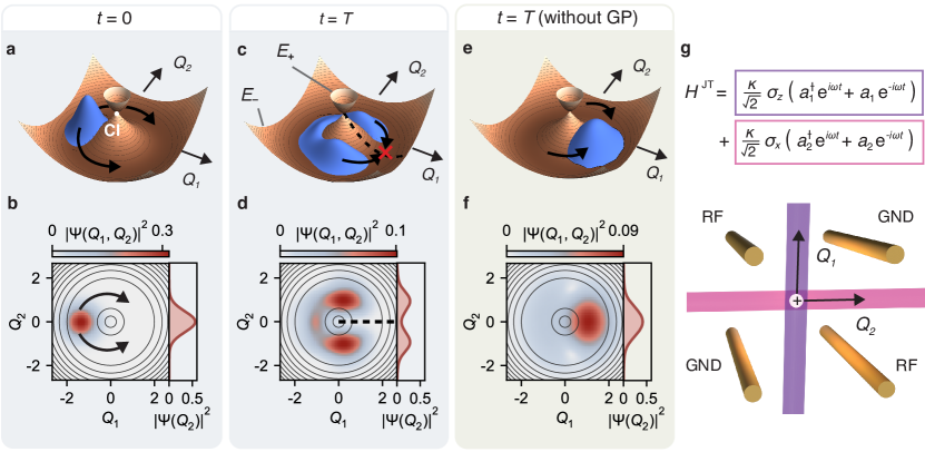
Figure 1: Directly detecting a geometric phase through wavepacket interference. a, A motional wavepacket is initially displaced to the minimum of the potential energy surface, after which it begins to encircle the conical intersection, denoted CI. b, Initial wavepacket density in 2D (left), and integrated over $Q_{1}$ (right). c, After sufficient time evolution, the two components of the wavepacket destructively interfere due to geometric phase, giving a nodal line along $Q_{2}=0$ (dotted line). d, Motional wavepacket density at the maximum interference time $T$. e, If the geometric phase were neglected, the two wavepacket components would interfere constructively. f, Density at $t=T$ with geometric phase neglected. Contours in b, d, and f correspond to the potential energy surface $E_{-}$. g, The Jahn-Teller Hamiltonian $H^{\mathrm{JT}}$ is engineered in an ion-trap quantum simulator with a single ^171Yb+ ion. The ion (white sphere) is confined in a Paul trap and $H^{\mathrm{JT}}$ is realised using two simultaneous laser-induced interactions (purple and pink, corresponding to colour-coded terms in $H^{\mathrm{JT}}$).

Here, we present the observation of the destructive interference caused by geometric phase during dynamics of a wavepacket around a conical intersection. We implement a controllable conical intersection by engineering a Jahn-Teller Hamiltonian in a trapped-ion quantum simulator that employs a mixed-qudit-boson (MQB) encoding in which both the ion’s electronic and motional degrees of freedom are used [38]. This work is not merely a simulation of geometric phase: the ion is a real, observable, and measurable quantum system that undergoes conical-intersection dynamics, allowing us to directly observe the geometric-phase interference of its motional wavepacket. To this end, our experiment introduces a resource-efficient reconstruction method to image the wavepacket’s probability density, directly showing the destructive self-interference as the wavepacket encircles a conical intersection. Experimental measurements match theoretical predictions, demonstrating the utility of quantum simulators to give insights into properties that have otherwise been impossible to measure directly for chemical systems.

Results

In an MQB simulator [38], the electronic and vibrational degrees of freedom that are to be simulated are represented in a qudit and a set of bosonic modes. We realise a conical intersection using an ^171Yb+ ion confined in a Paul trap, where two vibrations are encoded directly in the ion’s transverse vibrational modes (B₁ and B₂), while two electronic states are encoded in the ion’s qubit (qudit with $d=2$) states comprising the two hyperfine levels of the ^2S_1/2 ground state (detailed in Methods). This approach has recently been employed to predict molecular spectra using time-domain simulations [39], and provides resource-scaling advantages relative to conventional methods of quantum simulation [38].

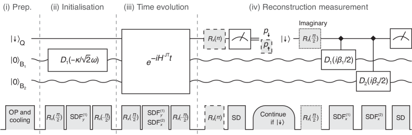
Figure 2: Experimental protocol for geometric-phase dynamics simulation and wavepacket reconstruction. (top) Quantum circuit diagram for a single-trapped-ion simulator, consisting of a qubit (Q, solid line) and 2 bosonic modes (B₁, B₂, wavy lines), and (bottom) corresponding experimental pulse sequence. (i) Preparation of fiducial states by optical pumping and cooling. (ii) Initialisation: B₁ is displaced by $D_{1}(-\kappa/\sqrt{2}\omega)$, implemented using an SDF pulse with surrounding qubit $\pi/2$ pulses to map to the correct basis. (iii) Time evolution under the Jahn-Teller Hamiltonian for duration $t$, implemented using two simultaneous SDF pulses in different bases, acting on the two bosonic modes. (iv) Reconstruction measurement: a state detection (SD) pulse collapses the qubit state, and the circuit proceeds only if the measured state was $\ket{\downarrow}$ (rounded shape). An additional single-qubit pulse (dashed) is introduced to retrieve information entangled with the $\ket{\uparrow}$ state. The qubit probabilities $p_{\downarrow}$ and $p_{\uparrow}$ are calculated from the mid-circuit measurement outcomes. Controlled displacements acting in the $\sigma_{x}$ basis (denoted ) map the motional degrees of freedom onto the qubit, allowing the real part of the characteristic function to be measured. Its imaginary part is obtained using an additional $R_{x}(\pi/2)$ pulse prior to the controlled displacements (dotted). Successive $R_{x}$ rotations shown separately in the circuit are combined into a single pulse in the experiment.

To demonstrate geometric-phase interference, we implement the $E\otimes e$ Jahn-Teller model [6], a standard model of geometric-phase effects in molecules [40, 8]. It consists of two electronic states coupled with two vibrational modes, described by the potential energy

$$V^{\mathrm{JT}}=\frac{\omega}{2}(Q_{1}^{2}+Q_{2}^{2})+\kappa(\sigma_{z}Q_{1}+\sigma_{x}Q_{2}),$$ (1)

where $\sigma_{x}$ and $\sigma_{z}$ are the Pauli matrices acting on the electronic states and $Q_{j}=(a_{j}^{{\dagger}}+a_{j})/\sqrt{2}$ is the dimensionless position coordinate for the $j$th vibrational mode, with creation and annihilation operators $a_{j}^{{\dagger}}$ and $a_{j}$. $\kappa$ is the vibronic coupling strength, and $\omega$ is the frequency of both vibrational modes. The Jahn-Teller Hamiltonian is given by $H^{\mathrm{JT}}=\omega(P_{1}^{2}+P_{2}^{2})/2+V^{JT}$, where $P_{j}$ is the conjugate momentum of $Q_{j}$. We set $\hbar=1$ throughout.

Diagonalisation of $V^{\mathrm{JT}}$ in the electronic basis leads to cylindrically symmetric potential energy surfaces along $Q_{1}$ and $Q_{2}$, with energies $E_{\pm}=\omega(Q_{1}^{2}+Q_{2}^{2})/2\pm\kappa\sqrt{Q_{1}^{2}+Q_{2}^{2}}$ (see fig. 1). The conical intersection is present at the point of highest symmetry ($Q_{1}=Q_{2}=0$), where the two potential energy surfaces are degenerate. The minimum of $E_{-}$ occurs where $Q_{1}^{2}+Q_{2}^{2}=(\kappa/\omega)^{2}$.

The effects of geometric phase on dynamics around a conical intersection can be directly observed from the motional probability density, fig. 1a–d. As the initial wavepacket, we choose the ground state of the non-interacting vibrational Hamiltonian, $H_{0}=\omega(a^{\dagger}_{1}a_{1}+a^{\dagger}_{2}a_{2})$, displaced to the potential-energy minimum at $Q_{1}=-\kappa/\omega$, $Q_{2}=0$ (fig. 1a–b). During the time evolution, the wavepacket splits into two components evolving in opposite directions around the conical intersection. The two components overlap at $Q_{1}>0$, causing destructive interference at the nodal line $Q_{2}=0$, where their equal and opposite geometric phases lead to a vanishing density (fig. 1c–d). By contrast, if geometric phase were disregarded, the two wavepacket fragments would interfere constructively, reaching maximum amplitude at $Q_{2}=0$ (fig. 1e–f).

To map the Jahn-Teller model onto the MQB simulator, we rewrite $H^{\textrm{JT}}$ in the interaction picture with respect to $H_{0}$,

$$H_{\mathrm{I}}^{\mathrm{JT}}={} \frac{\kappa}{\sqrt{2}}\sigma_{z}(a_{1}^{{\dagger}}e^{i\omega t}+a_{1}e^{-i\omega t})+$$

$$\frac{\kappa}{\sqrt{2}}\sigma_{x}(a_{2}^{{\dagger}}e^{i\omega t}+a_{2}e^{-i\omega t}),$$ (2)

which can be implemented using tunable light-atom interactions to enact qubit-boson couplings. We achieve this implementation using a coherent state-dependent force (SDF) enacted by stimulated Raman transitions driven with a $355\text{\,}\mathrm{n}\mathrm{m}$ pulsed laser [41, 42]. Driving transitions near bosonic mode $j$ leads to the Hamiltonian

$$H^{\mathrm{SDF}}_{j,\phi_{s}}(\delta,\Omega,\phi_{m})=\frac{\Omega}{2}\sigma_{\phi_{s}}(a_{j}^{\dagger}e^{i(\phi_{m}+\delta t)}+a_{j}e^{-i(\phi_{m}+\delta t)}),$$ (3)

where $\sigma_{\phi_{s}}=\sigma_{x}\cos\phi_{s}+\sigma_{y}\sin\phi_{s}$ and $\phi_{s}$ and $\phi_{m}$ are the phases associated with the qubit and the bosonic mode, respectively (see Methods). $\Omega$ and $\delta$ are the Rabi frequency and detuning of the laser from the bosonic mode, respectively. We use the notation $H^{\mathrm{SDF}}_{j,x}$ and $H^{\mathrm{SDF}}_{j,y}$ for SDF interactions where $\phi_{s}=0$ and $\phi_{s}=\pi/2$, respectively. Interactions in the $\sigma_{z}$ basis are obtained using a qubit basis rotation, $H^{\mathrm{SDF}}_{j,z}=R_{x}(\pi/2)H^{\mathrm{SDF}}_{j,y}R_{x}(-\pi/2)$, where $R_{x}(\theta)$ are driven qubit rotations around the Bloch sphere. $H^{\mathrm{JT}}$ can then be implemented in a programmable way using two simultaneous SDFs (see fig. 1g),

$$H^{\mathrm{JT}}_{\mathrm{I}}=H^{\mathrm{SDF}}_{1,z}(\omega,\sqrt{2}\kappa,0)+H^{\mathrm{SDF}}_{2,x}(\omega,\sqrt{2}\kappa,0).$$ (4)

The parameters $\kappa$ and $\omega$ are chosen to produce a clear wavepacket interference. To achieve this, $\kappa/\omega$ should be large enough that the wavepacket prepared at the minimum of the potential energy surface (at $Q_{1}=-\kappa/\omega$) has negligible overlap with the conical intersection. However, $\kappa/\omega$ should also be kept small enough to mitigate vibrational decoherence that increases with larger vibrational excitations. To balance these considerations, we choose $\kappa/\omega=1.5$, for which the wavepacket has only 1.7% of the density at $Q_{1}\geq 0$. $\kappa$, implemented by adjusting the Rabi frequency, is maximised to increase the speed of the dynamics; its value is constrained by the available SDF-laser power to $\kappa=2\pi\times$1.00\text{\,}\mathrm{k}\mathrm{H}\mathrm{z}$$, yielding $\omega=2\pi\times$667\text{\,}\mathrm{H}\mathrm{z}$$. With these parameters, the wavepackets are expected to experience the greatest geometric-phase interference at $T=$1.59\text{\,}\mathrm{m}\mathrm{s}$$, which was computationally predicted as half the time at which the width of the probability density is minimized.

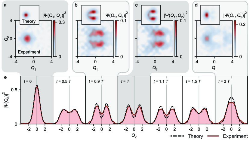
Figure 3: Wavepacket dynamics around an engineered conical intersection. a-d Reconstructed two-dimensional motional densities of the ^171Yb+ ion at times $t=0$, $0.9T$, $T$, and $2T$, with theoretical predictions in the insets. The nodal line at $Q_{2}=0$, $Q_{1}>0$ is a direct signature of geometric-phase interference. e One-dimensional motional densities (with the $Q_{1}$ coordinate integrated out) at more values of $t$. Geometric-phase interference causes the dip at $Q_{2}=0$ around $t=T$. The motional densities are obtained using eq. 5 (and its one-dimensional equivalent) from the characteristic functions, $\chi(i\beta_{1},i\beta_{2})$ and $\chi(i\beta_{2})$, measured using the circuit in fig. 2 (see Methods for details).

We probe the dynamics of the geometric phase around the conical intersection by reconstructing the ion’s motional probability densities at different evolution times $t$. The experimental sequence consists of four stages, shown in fig. 2. (i) Preparation of the qubit and cooling of the vibrational modes to their ground states is achieved by optical pumping, Doppler cooling, and sideband cooling. (ii) Initialisation consists of displacing B₁ to $Q_{1}=-\kappa/\omega$ by applying an SDF interaction $H^{\mathrm{SDF}}_{1,z}(0,\Omega_{1},\pi/2)$ for a duration $\tau$. This applies the displacement operator $D_{1}(-\Omega_{1}\tau/2)$, where $\Omega_{1}$ and $\tau$ are chosen to implement $D_{1}(-\kappa/\sqrt{2}\omega)$. (iii) Evolution of the system under $H^{\mathrm{JT}}_{I}$ is achieved by applying the two simultaneous SDF interactions of eq. 4 for an experimentally variable duration $t$. (iv) Reconstruction of the joint densities of B₁ and B₂ is achieved by measuring the characteristic function

$$\chi(i\beta_{1},i\beta_{2})=\bra{\Psi}D_{1}(i\beta_{1})D_{2}(i\beta_{2})\ket{\Psi},$$ (5)

where $\ket{\Psi}$ is the total wavefunction of the system, and $\beta_{1}$ and $\beta_{2}$ are real numbers. See Methods for details.

The joint probability densities are reconstructed using the circuit in fig. 2. Two SDF pulses are sequentially applied on B₁ and B₂, and $\chi(i\beta_{1},i\beta_{2})$ is scanned over $\beta_{1}$, $\beta_{2}$. These measurements yield the joint probability density via the Fourier transform of the measured characteristic function

$$|\Psi(Q_{1},Q_{2})|^{2}=\!\iint\frac{d\beta_{1}d\beta_{2}}{2\pi^{2}}e^{-i\sqrt{2}(Q_{1}\beta_{1}+Q_{2}\beta_{2})}\chi(i\beta_{1},i\beta_{2}).$$ (6)

In further detail, we measure $\chi(i\beta_{1},i\beta_{2})$ by mapping information from the multimode bosonic system onto the qubit using SDF pulses, moving beyond previous works on direct single-mode [43, 44, 45, 46] and indirect multimode reconstructions [47]. The reconstruction consists of preparing the qubit in $\ket{\downarrow}$ and applying two successive SDF interactions, $H^{\mathrm{SDF}}_{1,x}(0,\Omega_{2},0)$ and $H^{\mathrm{SDF}}_{2,x}(0,\Omega_{2},0)$ with durations $\tau_{1}$ and $\tau_{2}$. Doing so results in controlled displacements $D_{1}(i\beta_{1}/2)$ and $D_{2}(i\beta_{2}/2)$, where $\beta_{j}=\Omega_{2}\tau_{j}$. $\chi(i\beta_{1},i\beta_{2})$ is measured for different values of $\beta_{1}$ and $\beta_{2}$ by varying $\tau_{1}$ and $\tau_{2}$. We reconstruct the characteristic functions of the bosonic modes entangled with the $\ket{\downarrow}$ and $\ket{\uparrow}$ qubit states independently. Reconstructing the $\ket{\downarrow}$ component is achieved by adding a mid-circuit measurement which projects out the $\ket{\uparrow}$ component (see Methods). The experiment is repeated with an additional $R_{x}(\pi)$ pulse prior to the mid-circuit measurement to reconstruct the $\ket{\uparrow}$ component. The qubit probabilities $p_{\downarrow}$ and $p_{\uparrow}$ are calculated from the success rate of the mid-circuit measurement. After the displacements, measuring the qubit in the $\sigma_{z}$ basis gives the real part of the characteristic function, $\langle\sigma_{z}\rangle=\operatorname{Re}\chi(i\beta_{1},i\beta_{2})$. Repeating the experiment with an additional $R_{x}(\pi/2)$ pulse prior to the displacements gives the imaginary part, after which the full $\chi(i\beta_{1},i\beta_{2})$ is obtained by adding the real and imaginary parts associated with both $\ket{\downarrow}$ and $\ket{\uparrow}$.

The reconstructed probability densities in fig. 3a–d demonstrate a direct measurement of the wavepacket interference caused by the geometric phase. At $t=0$, the initial wavepacket is prepared at $(Q_{1},Q_{2})=(-1.5,0)$. As the wavepacket evolves around the conical intersection, the nodal line becomes visible at $Q_{2}=0$ and is most pronounced at $t=T$; this is a direct observation of destructive interference due to geometric phase. Finally, at $t=2T$, the two wavepackets recombine close to their initial position. The experimental results agree well with theoretical predictions, reproducing key features of interference and wavepacket recombination.

Further quantitative insight may be gained from the 1-dimensional density $|\Psi(Q_{2})|^{2}$, obtained by omitting the $D_{1}(i\beta_{1})$ displacements from the reconstruction procedure discussed earlier. In this case, the measurements scanned over $\beta_{2}$ are Fourier-transformed to give $|\Psi(Q_{2})|^{2}=\int d\beta_{2}\,e^{-i\sqrt{2}Q_{2}\beta_{2}}\chi(i\beta_{2})/\sqrt{2}\pi$. In fig. 3e, we present $|\Psi(Q_{2})|^{2}$ for seven different evolution times. A comparison of experiment and theory shows excellent agreement in the shape and amplitude of the measured density function. We attribute minor discrepancies to the dephasing of the bosonic modes, miscalibrations such as uncompensated AC Stark shifts, and technical imperfections in the protocol implementation.

Discussion

Our approach avoids the limitations of direct experiments on molecular systems, where only few observables—such as spectra and scattering cross sections—can be measured. Instead, a fully controllable quantum device—such as an ion-trap MQB simulator [38]—can, in principle, read out any observable; as we showed here, this includes the full two-dimensional density of the ^171Yb+ ion as it moves in space and time. A further advantage comes from the ratio ($r$) of the ion’s natural timescale (ms) and the measurement speed (ns), leading to an increase in the observable timing resolution of $r\sim 10^{6}$. This improves the achievable resolution of chemical-dynamics measurements relative to ultrafast observations.

A key general feature of quantum simulations is their programmability [48]. Our work is a simulation of the dynamics of the Jahn-Teller model, which is often used to describe molecular systems. In an MQB simulator, the qudit-boson interaction is controllable, meaning that the same device can be programmed to simulate different molecular systems, solid-state systems, or theoretical models that do not occur naturally. In particular, our geometric-phase simulator could be used to simulate dynamics in molecules with conical intersections where the interactions are not as symmetric as in $H^{\mathrm{JT}}$, such as the general quadratic vibronic-coupling Hamiltonian [38].

Like any analog simulation—quantum or classical—our approach is ultimately limited by noise and uncorrected errors. In our experiment, the main sources of decoherence and dissipation are motional dephasing and motional heating [49, 39] (see Methods). However, in MQB simulations of molecular processes, noise can be characterised and even amplified in order to create a realistic model of molecular environments, such as collisions in solution. Since our Jahn-Teller experiment shows only weak effects of decoherence over the full period $2T$, we would need to inject additional noise to simulate conical-intersection dynamics of real molecules in chemically realistic situations (i.e., other than a single molecule in vacuum). In scaling up to larger molecules, the ability to simulate dissipation would allow us to probe regimes in nonadiabatic dynamics that are among the most difficult to simulate on conventional computers [38].

Our methodology for probability density reconstruction enables scalability and resource efficiency. Early techniques for motional-state tomography were performed in the Fock basis [43, 50, 47], a process that requires many measurements if full motional densities are sought. More recently, wavepacket-reconstruction methods were developed based on the direct measurement of the characteristic function, significantly reducing the number of necessary measurements [46]. Our approach builds on the latter techniques, but has two additional advantages. First, we extend the characteristic-function method to multimode probability density reconstruction, while retaining both the requirement of few measurements and the ability to use one readout qubit. Second, using a mid-circuit measurement allows us to reuse the simulation qubit for the reconstruction, without any ancilla qubits.

We have recently become aware of related simultaneous work on simulating a conical intersection using a chain of trapped ions [51]. The system was adiabatically driven to its vibronic ground state, whose reconstructed two-dimensional density showed a node attributed to geometric phase. This work is complementary to ours in several ways: it focused on signatures of geometric phase in the ground state, not in the dynamics; it used Trotterised time evolution, while we drove the two interactions simultaneously; and it used an ancilla qubit in the reconstruction, while we used the mid-circuit-measurement approach discussed earlier.

In conclusion, our experiment represents the direct observation of wavepacket interference caused by geometric phase in dynamics around a conical intersection. Our approach to quantum simulation using an MQB trapped-ion system makes chemical dynamics that are otherwise unmeasurable directly accessible in the laboratory. This is a key demonstration of the utility of small-scale quantum computational devices to offer practical insights into chemical dynamics and resolve intractable problems in chemical physics.

Author Contributions Statement

RJM, IK, CH and TRT conceived the original idea; VCO, RJM, JBP, JY, and IK developed the theoretical methods; CHV, TN, ADR, MJM, and TRT developed and carried out the experiments; CHV, VCO, TRT, and IK wrote the manuscript with feedback from all authors; all authors discussed the results and interpreted the data.

Competing Interests Statement

The authors declare no competing interests.

Methods

Experimental setup

The ^171Yb^+ ion is confined in a Paul trap with radial mode oscillation frequencies of $2\pi\times$1.34\text{\,}\mathrm{M}\mathrm{H}\mathrm{z}$$ and $2\pi\times$1.47\text{\,}\mathrm{M}\mathrm{H}\mathrm{z}$$, corresponding to bosonic mode B₁ and B₂. The qubit is encoded in the two magnetically insensitive hyperfine levels of the ^2S_1/2 ground state, where we assign the labels $\ket{\downarrow}=\ket{F=0,m_{F}=0}$ and $\ket{\uparrow}=\ket{F=1,m_{F}=0}$.

We use two laser beams derived from a $355\text{\,}\mathrm{n}\mathrm{m}$ pulsed laser to coherently control the qubit and bosonic modes via stimulated Raman transitions within the ^2S_1/2 ground state. The two Raman beams are orthogonal to one another, and configured so that they can be coupled to both radial vibrational modes. Each Raman beam passes through an acousto-optical modulator (AOM), which allows the phase, frequency and amplitude of the beam to be adjusted by altering the RF signal driving the AOM. One of the RF signals is generated by an arbitrary waveform generator (Keysight M8190A), allowing multiple phase-coherent tones to be imprinted on one of the laser beams. We ensure phase coherence between all pulses in the experimental sequence by tracking the phase (relative to the beginning of the pulse sequence) and applying appropriate corrections.

By tuning the frequency difference of the Raman beams, one can drive carrier, red- and blue-sideband transitions. Qubit rotations are obtained by driving carrier transitions, while an SDF $H^{\mathrm{SDF}}_{j,\phi_{s}}(0,\Omega,\phi_{m})$ arises from combining the red- and blue-sideband transitions. Applying this interaction for a duration $\tau$ with the qubit in an eigenstate of $\sigma_{\phi_{s}}$ displaces bosonic mode $j$ by $D_{j}(\alpha)=\exp(\alpha a^{\dagger}_{j}-\alpha^{*}a_{j})$, where $\alpha=-i\Omega\tau e^{i\phi_{m}}/2$. The amplitude and phase-space direction of the displacement are adjusted by varying $\tau$ and $\phi_{m}$, respectively.

Experimental protocol

Preparation. The bosonic modes are cooled in two stages. First, they are Doppler cooled using a $369.5\text{\,}\mathrm{n}\mathrm{m}$ laser red-detuned from the ^2S_1/2 $\rightarrow$ ^2P_1/2 transition. Second, resolved sideband cooling is used to reach their motional ground states, achieving temperatures of $\bar{n}=0.04$ measured via sideband thermometry [1]. The qubit is prepared in its ground state $\ket{\downarrow}$ via optical pumping, using another $369.5\text{\,}\mathrm{n}\mathrm{m}$ laser resonant with the ^2S_1/2 $\ket{F=1}$ $\rightarrow$ ^2P_1/2 $\ket{F=1}$ transition.

Initialisation. To initialise B₁, we apply an SDF interaction $H^{\mathrm{SDF}}_{1,y}(0,\Omega_{1},\pi/2)$ for a duration $\tau$, which gives a displacement $D_{1}(\alpha)$ where $\alpha=\Omega_{1}\tau/2$. Setting $\tau=\sqrt{2}\kappa/\omega\Omega_{1}$ so that $\alpha=\kappa/\sqrt{2}\omega$ displaces the mode from $Q_{1}=0$ to $Q_{1}=-\kappa/\omega$ because $D_{1}(\alpha)Q_{1}D_{1}(\alpha)^{\dagger}=Q_{1}-\sqrt{2}\operatorname{Re}\alpha=Q_{1}-\kappa/\omega$. The qubit is first mapped into the SDF interaction basis ($\ket{+}_{y}$) with an $R_{x}(\pi/2)$ rotation, and is returned to $\ket{\downarrow}$ after the displacement with an $R_{x}(-\pi/2)$ rotation. The Rabi frequency of the SDF interaction was frequently recalibrated and on average we measured $\Omega_{1}=2\pi\times$2.23\text{\,}\mathrm{k}\mathrm{H}\mathrm{z}$$.

Time evolution. Two SDF interactions on B₁ and B₂ are applied during the time evolution. Their measured Rabi frequencies were, on average, $\sqrt{2}\kappa=2\pi\times$1.42\text{\,}\mathrm{k}\mathrm{H}\mathrm{z}$$ and are calibrated within 2% of each other. The duration $T$ of the geometric-phase dynamics is scaled according to the calibrated Rabi frequency.

Reconstruction measurement. After the simulated time evolution, the system is in the entangled state $\ket{\Psi}=a_{\downarrow}\ket{\downarrow}\ket{\psi_{\downarrow}}_{B_{1}}\ket{\xi_{\downarrow}}_{B_{2}}+a_{\uparrow}\ket{\uparrow}\ket{\psi_{\uparrow}}_{B_{1}}\ket{\xi_{\uparrow}}_{B_{2}}$. In preparation of the reconstruction, a mid-circuit measurement projects the qubit state to either $\ket{\downarrow}$ or $\ket{\uparrow}$ through state-dependent fluorescence induced by a $369.5\text{\,}\mathrm{n}\mathrm{m}$ laser beam resonant with the ^2S_1/2 $\ket{F=1}$ $\rightarrow$ ^2P_1/2 $\ket{F=0}$ transition. The qubit states are inferred by thresholding the number of photons collected on an avalanche photodiode (measured state preparation and measurement fidelity of 99.5%), and the outcomes of the measurement determine the probabilities $p_{\downarrow}=|a_{\downarrow}|^{2}$ and $p_{\uparrow}=|a_{\uparrow}|^{2}$. A measurement outcome of $\ket{\uparrow}$ induces significant decoherence of the bosonic modes due to photon recoils. Therefore, the reconstruction only proceeds if the measurement outcome is $\ket{\downarrow}$, for which no photon is emitted. Doing so projects the bosonic modes to $\ket{\psi_{\downarrow}}_{B_{1}}\ket{\xi_{\downarrow}}_{B_{2}}$. To retrieve $\ket{\psi_{\uparrow}}_{B_{1}}\ket{\xi_{\uparrow}}_{B_{2}}$ instead, we insert an $R_{x}(\pi)$ pulse that flips the qubit before the measurement. After the mid-circuit measurement, the characteristic functions $\chi_{\downarrow}(i\beta_{1},i\beta_{2})$ and $\chi_{\uparrow}(i\beta_{1},i\beta_{2})$ corresponding to each qubit state are measured as described in the main text. The full characteristic function is then the sum of both contributions, $\chi(i\beta_{1},i\beta_{2})=p_{\downarrow}\chi_{\downarrow}(i\beta_{1},i\beta_{2})+p_{\uparrow}\chi_{\uparrow}(i\beta_{1},i\beta_{2})$. The values $\beta_{j}=\Omega_{2}\tau_{j}$ are scanned by varying the SDF-pulse duration $\tau_{j}$. The Rabi frequency was recalibrated between experiments and, on average, $\Omega_{2}=2\pi\times$2.31\text{\,}\mathrm{k}\mathrm{H}\mathrm{z}$$, resulting in combined pulse durations of up to $553\text{\,}\mathrm{\SIUnitSymbolMicro}\mathrm{s}$. We measured $\chi(i\beta_{2})$ for $\beta_{2}\in[0,5]$ and $\chi(i\beta_{1},i\beta_{2})$ for $\beta_{1},\beta_{2}\in[0,4]$ by varying the SDF pulse durations. Since the characteristic function is Hermitian, $\chi(i\beta_{1},i\beta_{2})^{*}=\chi(-i\beta_{1},-i\beta_{2})$, we used symmetry to find $\chi(i\beta_{2})$ for $\beta_{2}<0$ and $\chi(i\beta_{1},\beta_{2})$ for $\beta_{1}<0$ or $\beta_{2}<0$. We did not measure the vanishing imaginary part of $\chi(i\beta_{2})$ nor $\chi_{\downarrow}$ at $t=0$. The measured characteristic functions are shown in Extended Data Fig. 1.

Data acquisition. The characteristic functions were measured in a way to average out the effects of drift. In each run of the experiment, we randomised the order of the displacement-pulse durations in which $\chi$ was reconstructed. For each run, the quantum circuit to obtain $\chi_{\downarrow}$ and $\chi_{\uparrow}$ was repeated until the mid-circuit measurement succeeded 500 times, resulting in 500 measurement repetitions of the reconstruction routine and 1000 measurements to obtain a value of the full $\chi$. Furthermore, the order of the displacements was randomised. Overall, each of the 1- and 2-dimensional experiments was repeated, respectively, four and two times and the results of the runs averaged for a total of 2000 and 1000 measurements for each duration. The bosonic mode frequencies were calibrated every $6\text{\,}\mathrm{m}\mathrm{i}\mathrm{n}$, while the full system parameters were recalibrated after the second experimental run. The 1-dimensional and the four 2-dimensional ($t=\{0,0.9T,T,2T\}$) experiments were done on five separate days with total durations of 15.6, 2.8, 8.8, 8.7 and 10.6 hours, respectively.

Noise sources Decoherence of the bosonic modes, made up of motional heating and dephasing, was the dominant noise mechanism in our system. Motional heating was caused by electric field noise at the radial mode frequency, while motional dephasing arose from fluctuations in the harmonic trapping potential strength [2]. We measured the heating rate and the motional dephasing time of B₁ (representative for both modes) to be $\dot{\bar{n}}=$0.2\text{\,}\mathrm{q}\mathrm{u}\mathrm{a}\mathrm{n}\mathrm{t}\mathrm{a}\leavevmode\nobreak\ \mathrm{s}^{-1}$$ and $T_{2}^{*}=$35\text{\,}\mathrm{m}\mathrm{s}$$ [39]. The motional coherence was limited by noise in the radio frequency (RF) trapping voltage, which was actively stabilised to mitigate fluctuations in the radial mode frequencies. Slow drifts of the trapping voltage were compensated for with frequent motional mode recalibrations.

Characteristic functions

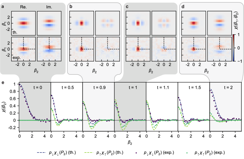
Extended Data Fig. 1: Characteristic functions of the wavepacket measured for various evolution times. a-d Joint two-dimensional characteristic function $\chi(i\beta_{1},i\beta_{2})=p_{\downarrow}\chi_{\downarrow}(i\beta_{1},i\beta_{2})+p_{\uparrow}\chi_{\uparrow}(i\beta_{1},i\beta_{2})$ measured at times $t=\{0,0.9T,T,2T\}$ using the full pulse sequence of fig. 2. The real (left) and imaginary (right) parts are measured with and without an $R_{x}(\pi/2)$ pulse in the reconstruction. The top row shows theoretical predictions and the bottom experimental results. $\chi(i\beta_{1},i\beta_{2})$ were measured in the range $\beta_{1},\beta_{2}\in[0,4]$ with $11\times 11$ equidistant samples (dashed quadrant). Values in the remaining three quadrants are obtained from the symmetry of $\chi(i\beta_{1},i\beta_{2})$. e One-dimensional characteristic functions $\chi_{\downarrow}(i\beta_{2})$ and $\chi_{\uparrow}(i\beta_{2})$ obtained by omitting displacements on B₁ in the reconstruction. $\beta_{2}$ was uniformly sampled in the range $[0,5]$ with 26 points. Each two- and one-dimensional characteristic function was averaged over 1000 and 2000 measurements, respectively. Error bars in e represent one standard deviation based on quantum projection noise.

Figure 1 shows the measured characteristic functions used to reconstruct the wavepacket probability densities. The two-dimensional characteristic functions (fig. 1a–d) require four measurements at each $t$ to obtain the real and imaginary parts of $p_{\downarrow}\chi_{\downarrow}(i\beta_{1},i\beta_{2})$ and $p_{\uparrow}\chi_{\uparrow}(i\beta_{1},i\beta_{2})$. The one-dimensional characteristic functions (fig. 1e) require two measurements to determine $p_{\downarrow}\chi_{\downarrow}(i\beta_{2})$ and $p_{\uparrow}\chi_{\uparrow}(i\beta_{2})$, as the vanishing imaginary part is not measured. In both one- and two-dimensional reconstructions, only positive values of $\beta_{1}$ and $\beta_{2}$ are sampled; the characteristic function in other ranges is obtained by symmetry.

We performed post-processing to remove artifacts associated with Fourier transformations between a characteristic function and its probability density. A non-zero DC offset appearing as background noise in the characteristic functions propagates into the probability densities at the origin [46]. Since background noise with a non-zero mean is a technical imperfection and is independent of the geometric-phase evolution, we correct for it in post-processing. We estimate the mean of the background noise by averaging $\chi(i\beta_{1},i\beta_{2})$ with $\sqrt{\beta_{1}^{2}+\beta_{1}^{2}}\geq 3.6$ for the two-dimensional and $\chi(i\beta_{2})$ with $\beta_{2}\geq 3.6$ for the one-dimensional case, and offset the data by the negative of this average. This baseline correction was on average 0.02, with the largest correction of 0.03.

Phase coherence in the pulse sequence

This appendix describes the experimental procedure to track the qubit and motional phases, ensuring phase coherence between sequential spin-motional interactions.

The laser-induced excitations interacting with an ion with a qubit frequency $\omega_{0}$ and a motional mode with frequency $\omega_{m}$ are the carrier (c), red-sideband (rsb), and blue-sideband transitions (bsb). Their interaction Hamiltonians, after dropping high-frequency terms, are

$$H_{\textrm{c}} =\frac{\Omega_{c}}{2}\sigma^{+}e^{i\phi_{c}}e^{i(\omega_{c}-\omega_{0})t}+\textrm{h.c.},$$ (7)

$$H_{\textrm{rsb}} =\frac{\eta\Omega_{r}}{2}\sigma^{+}ae^{i\phi_{r}}e^{i(\omega_{r}-\omega_{0}+\omega_{m})t)}+\textrm{h.c.},$$ (8)

$$H_{\textrm{bsb}} =\frac{\eta\Omega_{b}}{2}\sigma^{+}a^{\dagger}e^{i\phi_{b}}e^{i(\omega_{b}-\omega_{0}-\omega_{m})t)}+\textrm{h.c.},$$ (9)

where $\eta$ is the Lamb-Dicke parameter and $\Omega_{c,b,r}$ are the respective Rabi frequencies. $\omega_{c,b,r}$ and $\phi_{c,b,r}$ correspond, respectively, to the frequency differences and the phase differences of the two orthogonal Raman beams. Simultaneously driving the red- and blue-sidebands with $\Omega=\eta\Omega_{r}=\eta\Omega_{b}$ gives

$$H_{\textrm{SDF}} =H_{\textrm{rsb}}+ H_{\textrm{bsb}}$$

$$=\frac{\Omega}{2}\sigma^{+}[ ae^{i\phi_{r}}e^{i(\omega_{r}-\omega_{0}+\omega_{m})t}+{}$$

$$a^{\dagger}e^{i\phi_{b}}e^{i(\omega_{b}-\omega_{0}-\omega_{m})t}+\textrm{h.c.}].$$ (10)

We consider $\omega_{r}$ and $\omega_{b}$ to be set near-resonant with the red- and blue-sideband transitions,

$$\omega_{r} =\omega_{0}-\omega_{m}-\delta\omega_{m}+\delta\omega_{0},$$ (11)

$$\omega_{b} =\omega_{0}+\omega_{m}+\delta\omega_{m}+\delta\omega_{0},$$ (12)

where $\delta\omega_{0}$ is an asymmetrical (center-line) detuning from the qubit frequency, and $\delta\omega_{m}$ is a symmetrical detuning from the motional mode frequency. With the spin phase $\phi_{s}=(\phi_{r}+\phi_{b})/2$ and the motional phase $\phi_{m}=(\phi_{b}-\phi_{r})/2$, eq. 10 can be rewritten as

$$H_{\textrm{SDF}}=\frac{\Omega}{2}\sigma^{+}e^{i(\delta\omega_{0}t+\phi_{s})}[ ae^{-i(\delta\omega_{m}t+\phi_{m})}+$$

$$a^{\dagger}e^{i(\delta\omega_{m}t+\phi_{m})}]+\textrm{h.c.}$$ (13)

This Hamiltonian corresponds to eq. 3 in the main text by setting $\delta\omega_{0}=0$ and $\delta\omega_{m}=\delta$. The motional phase $\phi_{m}$ can be adjusted to selectively displace a mode along $Q$ or $P$. Equation 13 shows that non-zero or miscalibrated $\delta\omega_{0}$ and $\delta\omega_{m}$ introduce a time-dependent phase offset to $\phi_{s}$ and $\phi_{m}$ which, if uncorrected, will lead to incorrect interactions.

The qubit frequency detuning is, from eq. 11 and eq. 12, $\delta\omega_{0}=(\omega_{b}+\omega_{r})/2-\omega_{0}$. To avoid phase lags associated with $\phi_{s}$, we enforce $(\omega_{b}+\omega_{r})/2=\omega_{c}=\bar{\omega}_{0}$ for all pulses throughout the entire circuit, namely single-qubit rotations and SDF interactions on B₁ and B₂. Here, $\bar{\omega}_{0}$ indicates the qubit frequency measured via a Ramsey sequence in a separate calibration experiment.

Likewise, eq. 11 and eq. 12 give the motional detuning as $\delta\omega_{m}=(\omega_{b}-\omega_{r})/2-\omega_{m}$. To avoid unwanted phase lags associated with $\phi_{m}$, we enforce $(\omega_{b}-\omega_{r})/2=\bar{\omega}_{m}$ for all SDF pulses throughout the circuit, where $\bar{\omega}_{m}$ is the experimentally measured motional frequency. There is an unavoidable phase lag due to the detuning $\delta$ required in the SDF interactions during the time evolution. To correct this, we add a motional phase offset of $\tau_{1}\delta$ to the SDF interaction during the initial displacement, where $\tau_{1}$ is the duration of the initialisation. Furthermore, a motional phase offset of $(t+\tau_{1})\delta$ is added to the reconstruction SDF pulses, where $t$ is the duration of the time evolution.

Calibration of motional frequencies

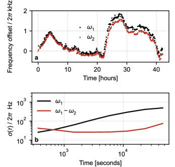
Extended Data Fig. 2: Frequency drifts of radial motional modes. a Time series of motional frequencies $\omega_{1,2}$ corresponding to B_1,2, measured using the calibration routine detailed in the text and plotted as the frequency offset from $\omega_{1}$ measured at $t=0$. b Allan deviation of $\omega_{1}$, and of the difference between the two frequencies ($\omega_{1}-\omega_{2}$).

We used a calibration scheduling routine to recalibrate parameters during each experiment and ensure high-fidelity implementations of the pulse sequence. Moreover, we optimised the scheduler to maximise the experimental duty cycle by analysing the temporal noise behaviours.

The data quality of the reconstructed densities depends on correctly setting the laser frequencies for the motional sideband interactions that enact SDF interactions. The motional frequencies $\omega_{1}$ and $\omega_{2}$ associated with B₁ and B₂ are calibrated as previously reported [39]. To do so, both SDF interactions are applied, but we set the fields associated with $\omega_{2}$ to be sufficiently off resonant while calibrating $\omega_{1}$. We prepare the state $\ket{\downarrow}\ket{0}_{\textrm{B}_{1}}$ and apply two sequential SDF pulses with a relative phase shift $\phi_{m}=\pi$. In the absence of frequency errors, the mode returns to its original state and a qubit measurement yields zero population in $\ket{\uparrow}$. However, in the presence of errors, the motion remains entangled with the qubit, giving a non-zero measured probability. The SDF fields’ frequencies are then scanned, and a fit to the measurements yields the correct mode frequency. We repeat this procedure to calibrate $\omega_{2}$ by setting the SDF field associated with $\omega_{1}$ to be off resonant.

Figure 2 shows the drifts in the radial mode frequencies over time, which varied in a range of $2\pi\times$2.2\text{\,}\mathrm{k}\mathrm{H}\mathrm{z}$$ over 2 days. From numerical simulations, we determined that an error tolerance of about $10\%$ is required for the detuning ($\delta\simeq 2\pi\times$667\text{\,}\mathrm{H}\mathrm{z}$$) in the time evolution to obtain adequate results. Given that typical experiments lasted tens of hours, frequent recalibrations of the motional mode frequencies were necessary. To this end, we implemented a scheduling algorithm to interleave calibrations and experiments [3]. The scheduling rate was determined by choosing a time interval for which the Allan deviation was sufficiently small. From fig. 2b, we chose an interval of 6 minutes, corresponding to an Allan deviation of $2\pi\times$26\text{\,}\mathrm{H}\mathrm{z}$$ and satisfying the required tolerance. We also found highly correlated noise between the radial modes (see Extended Data Fig. 2), suggesting a common noise source (e.g., trap RF amplitude fluctuations). Therefore, to increase the experiment duty cycle, frequency offsets measured on B₁ were also used to correct for B₂.

Data Availability

A repository containing data plotted in Fig. 3 and in Extended Data Fig. 1 is available at https://doi.org/10.5281/zenodo.7955887 ([4])

References

- Yarkony [1996] D. R. Yarkony, Diabolical conical intersections, Rev. Mod. Phys. 68, 985 (1996).
- Domcke et al. [2004] W. Domcke, D. R. Yarkony, and H. Köppel, Conical Intersections: Electronic Structure, Dynamics and Spectroscopy (World Scientific Publishing, 2004).
- Larson et al. [2020] J. Larson, E. Sjöqvist, and P. Öhberg, Conical Intersections in Physics (Springer Cham, 2020).
- Domcke and Yarkony [2012] W. Domcke and D. R. Yarkony, Role of conical intersections in molecular spectroscopy and photoinduced chemical dynamics, Annu. Rev. Phys. Chem. 63, 325 (2012).
- Berry [1984] M. V. Berry, Quantal phase factors accompanying adiabatic changes, Proc. R. Soc. Lond. A 392, 47 (1984).
- Longuet-Higgins et al. [1958] H. C. Longuet-Higgins, U. Öpik, M. H. L. Pryce, and R. A. Sack, Studies of the Jahn-Teller effect II. The dynamical problem, Proc. R. Soc. Lond. A 244, 1 (1958).
- Mead and Truhlar [1979] C. A. Mead and D. G. Truhlar, On the determination of Born–Oppenheimer nuclear motion wave functions including complications due to conical intersections and identical nuclei, J. Chem. Phys. 70, 2284 (1979).
- Schön and Köppel [1995] J. Schön and H. Köppel, Geometric phase effects and wave packet dynamics on intersecting potential energy surfaces, J. Chem. Phys. 103, 9292 (1995).
- Ryabinkin et al. [2017] I. G. Ryabinkin, L. Joubert-Doriol, and A. F. Izmaylov, Geometric phase effects in nonadiabatic dynamics near conical intersections, Acc. Chem. Res. 50, 1785 (2017).
- Mead [1980] C. A. Mead, Superposition of reactive and nonreactive scattering amplitudes in the presence of a conical intersection, J. Chem. Phys. 72, 3839 (1980).
- Lepetit and Kuppermann [1990] B. Lepetit and A. Kuppermann, Numerical study of the geometric phase in the \ceH + H2 reaction, Chem. Phys. Lett. 166, 581 (1990).
- Althorpe [2006] S. C. Althorpe, General explanation of geometric phase effects in reactive systems: Unwinding the nuclear wave function using simple topology, J. Chem. Phys. 124, 084105 (2006).
- Althorpe et al. [2008] S. C. Althorpe, T. Stecher, and F. Bouakline, Effect of the geometric phase on nuclear dynamics at a conical intersection: Extension of a recent topological approach from one to two coupled surfaces, J. Chem. Phys. 129, 214117 (2008).
- Kendrick [1997] B. Kendrick, Geometric phase effects in the vibrational spectrum of \ceNa3(X), Phys. Rev. Lett. 79, 2431 (1997).
- Applegate et al. [2003] B. E. Applegate, T. A. Barckholtz, and T. A. Miller, Explorations of conical intersections and their ramifications for chemistry through the Jahn–Teller effect, Chem. Soc. Rev. 32, 38 (2003).
- Englman [2016] R. Englman, Spectroscopic detectability of the molecular Aharonov-Bohm effect, J. Chem. Phys. 144, 024103 (2016).
- Yuan et al. [2018] D. Yuan, Y. Guan, W. Chen, H. Zhao, S. Yu, C. Luo, Y. Tan, T. Xie, X. Wang, Z. Sun, D. H. Zhang, and X. Yang, Observation of the geometric phase effect in the \ceH + HD →H2 + D reaction, Science 362, 1289 (2018).
- Yuan et al. [2020] D. Yuan, Y. Huang, W. Chen, H. Zhao, S. Yu, C. Luo, Y. Tan, S. Wang, X. Wang, Z. Sun, and X. Yang, Observation of the geometric phase effect in the \ceH + HD →H2 + D reaction below the conical intersection, Nat. Commun. 11, 3640 (2020).
- Cina and Romero-Rochin [1990] J. A. Cina and V. Romero-Rochin, Optical impulsive excitation of molecular pseudorotation in Jahn–Teller systems, J. Chem. Phys. 93, 3844 (1990).
- Cina [1991] J. A. Cina, Phase-controlled optical pulses and the adiabatic electronic sign change, Phys. Rev. Lett. 66, 1146 (1991).
- Cina et al. [1993] J. A. Cina, J. T. J. Smith, and V. Romero-Rochin, Time-resolved optical tests for electronic geometric phase development, Adv. in Chem. Phys. 83, 1 (1993).
- Castro Neto et al. [2009] A. H. Castro Neto, F. Guinea, N. M. R. Peres, K. S. Novoselov, and A. K. Geim, The electronic properties of graphene, Rev. Mod. Phys. 81, 109 (2009).
- Ran et al. [2009] Y. Ran, F. Wang, H. Zhai, A. Vishwanath, and D.-H. Lee, Nodal spin density wave and band topology of the FeAs-based materials, Phys. Rev. B 79, 014505 (2009).
- Rashba [1959] E. Rashba, Symmetry of energy bands in crystals of wurtzite type: I. symmetry of bands disregarding spin-orbit interaction, Sov. Phys.-Solid State 1, 368 (1959).
- Dresselhaus [1955] G. Dresselhaus, Spin-orbit coupling effects in zinc blende structures, Phys. Rev. 100, 580 (1955).
- Cina [2008] J. A. Cina, Wave-packet interferometry and molecular state reconstruction: Spectroscopic adventures on the left-hand side of the Schrödinger equation, Annu. Rev. Phys. Chem. 59, 319 (2008).
- Buluta and Nori [2009] I. Buluta and F. Nori, Quantum simulators, Science 326, 108 (2009).
- Blatt and Roos [2012] R. Blatt and C. F. Roos, Quantum simulations with trapped ions, Nat. Phys. 8, 277 (2012).
- Aspuru-Guzik and Walther [2012] A. Aspuru-Guzik and P. Walther, Photonic quantum simulators, Nat. Phys. 8, 285 (2012).
- McArdle et al. [2020] S. McArdle, S. Endo, A. Aspuru-Guzik, S. C. Benjamin, and X. Yuan, Quantum computational chemistry, Rev. Mod. Phys. 92, 015003 (2020).
- Gorman et al. [2018] J. D. Gorman, B. Hemmerling, E. Megidish, S. A. Moeller, P. Schindler, M. Sarovar, and H. Haeffner, Engineering vibrationally assisted energy transfer in a trapped-ion quantum simulator, Phys. Rev. X 8, 011038 (2018).
- Duca et al. [2015] L. Duca, T. Li, M. Reitter, I. Bloch, M. Schleier-Smith, and U. Schneider, An Aharonov-Bohm interferometer for determining Bloch band topology, Science 347, 288 (2015).
- Brown et al. [2022] C. D. Brown, S.-W. Chang, M. N. Schwarz, T.-H. Leung, V. Kozii, A. Avdoshkin, J. E. Moore, and D. Stamper-Kurn, Direct geometric probe of singularities in band structure, Science 377, 1319 (2022).
- Gambetta et al. [2021] F. M. Gambetta, C. Zhang, M. Hennrich, I. Lesanovsky, and W. Li, Exploring the many-body dynamics near a conical intersection with trapped Rydberg ions, Phys. Rev. Lett. 126, 233404 (2021).
- Dereli et al. [2012] T. Dereli, Y. Gül, P. Forn-Díaz, and O. E. Müstecaplıoğlu, Two-frequency Jahn-Teller systems in circuit QED, Phys. Rev. A 85, 053841 (2012).
- Larson [2008] J. Larson, Jahn-Teller systems from a cavity QED perspective, Phys. Rev. A 78, 033833 (2008).
- Wang et al. [2023] C. S. Wang, N. E. Frattini, B. J. Chapman, S. Puri, S. M. Girvin, M. H. Devoret, and R. J. Schoelkopf, Observation of wave-packet branching through an engineered conical intersection, Phys. Rev. X 13, 011008 (2023).
- MacDonell et al. [2021] R. J. MacDonell, C. E. Dickerson, C. J. T. Birch, A. Kumar, C. L. Edmunds, M. J. Biercuk, C. Hempel, and I. Kassal, Analog quantum simulation of chemical dynamics, Chem. Sci. 12, 9794 (2021).
- MacDonell et al. [2022] R. J. MacDonell, T. Navickas, T. F. Wohlers-Reichel, C. H. Valahu, A. D. Rao, M. J. Millican, M. A. Currington, M. J. Biercuk, T. R. Tan, C. Hempel, and I. Kassal, Predicting molecular vibronic spectra using time-domain analog quantum simulation, arXiv:2209.06558 (2022).
- Bersuker [2001] I. B. Bersuker, Modern aspects of the Jahn-Teller effect: Theory and applications to molecular problems, Chem. Rev. 101, 1067 (2001).
- Monroe et al. [1996] C. Monroe, D. M. Meekhof, B. E. King, and D. J. Wineland, A “Schrödinger cat” superposition state of an atom, Science 272, 1131 (1996).
- Mizrahi et al. [2013] J. Mizrahi, B. Neyenhuis, K. G. Johnson, W. C. Campbell, C. Senko, D. Hayes, and C. Monroe, Quantum control of qubits and atomic motion using ultrafast laser pulses, Appl. Phys. B 114, 45 (2013).
- Leibfried et al. [1996] D. Leibfried, D. M. Meekhof, B. E. King, C. Monroe, W. M. Itano, and D. J. Wineland, Experimental determination of the motional quantum state of a trapped atom, Phys. Rev. Lett. 77, 4281 (1996).
- Gerritsma et al. [2010] R. Gerritsma, G. Kirchmair, F. Zähringer, E. Solano, R. Blatt, and C. F. Roos, Quantum simulation of the Dirac equation, Nature 463, 68 (2010).
- Johnson et al. [2015] K. G. Johnson, B. Neyenhuis, J. Mizrahi, J. D. Wong-Campos, and C. Monroe, Sensing atomic motion from the zero point to room temperature with ultrafast atom interferometry, Phys. Rev. Lett. 115, 213001 (2015).
- Flühmann and Home [2020] C. Flühmann and J. P. Home, Direct characteristic-function tomography of quantum states of the trapped-ion motional oscillator, Phys. Rev. Lett. 125, 043602 (2020).
- Jia et al. [2022] Z. Jia, Y. Wang, B. Zhang, J. Whitlow, C. Fang, J. Kim, and K. R. Brown, Determination of multimode motional quantum states in a trapped ion system, Phys. Rev. Lett. 129, 103602 (2022).
- Hayes et al. [2014] D. Hayes, S. T. Flammia, and M. J. Biercuk, Programmable quantum simulation by dynamic Hamiltonian engineering, New J. Phys. 16, 083027 (2014).
- Brownnutt et al. [2015] M. Brownnutt, M. Kumph, P. Rabl, and R. Blatt, Ion-trap measurements of electric-field noise near surfaces, Rev. Mod. Phys. 87, 1419 (2015).
- Kienzler et al. [2016] D. Kienzler, C. Flühmann, V. Negnevitsky, H.-Y. Lo, M. Marinelli, D. Nadlinger, and J. P. Home, Observation of quantum interference between separated mechanical oscillator wave packets, Phys. Rev. Lett. 116, 140402 (2016).
- Whitlow et al. [2022] J. Whitlow, Z. Jia, Y. Wang, C. Fang, J. Kim, and K. R. Brown, Simulating conical intersections with trapped ions, arXiv:2211.07319 (2022).

References

- Monroe et al. [1995] C. Monroe, D. M. Meekhof, B. E. King, S. R. Jefferts, W. M. Itano, D. J. Wineland, and P. Gould, Resolved-sideband Raman cooling of a bound atom to the 3D zero-point energy, Phys. Rev. Lett. 75, 4011 (1995).
- Wineland et al. [1998] D. J. Wineland, C. Monroe, W. M. Itano, D. Leibfried, B. E. King, and D. M. Meekhof, Experimental issues in coherent quantum-state manipulation of trapped atomic ions, J. Res. Natl. Inst. Stand. Technol. 103, 259 (1998).
- Riesebos et al. [2021] L. Riesebos, B. Bondurant, and K. R. Brown, Universal graph-based scheduling for quantum systems, IEEE Micro 41, 5 (2021).
- Valahu et al. [2023] C. H. Valahu, V. C. Olaya-Agudelo, R. J. MacDonell, T. Navickas, A. D. Rao, M. J. Millican, J. Pérez-Sánchez, J. Yuen-Zhou, M. J. Biercuk, C. Hempel, T. R. Tan, and I. Kassal, Direct observation of geometric phase in dynamics around a conical intersection [Dataset], Zenodo https://doi.org/10.5281/zenodo.7955887 (2023).