SVS: Adversarial refinement
for sparse novel view synthesis

Abstract

This paper proposes Sparse View Synthesis. This is a view synthesis problem where the number of reference views is limited, and the baseline between target and reference view is significant. Under these conditions, current radiance field methods fail catastrophically due to inescapable artifacts such 3D floating blobs, blurring and structural duplication, whenever the number of reference views is limited, or the target view diverges significantly from the reference views.

Advances in network architecture and loss regularisation are unable to satisfactorily remove these artifacts. The occlusions within the scene ensure that the true contents of these regions is simply not available to the model. In this work, we instead focus on hallucinating plausible scene contents within such regions. To this end we unify radiance field models with adversarial learning and perceptual losses. The resulting system provides up to 60% improvement in perceptual accuracy compared to current state-of-the-art radiance field models on this problem.

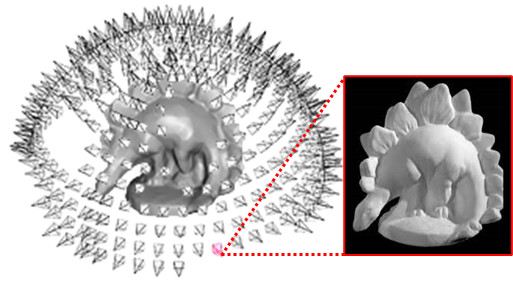
(a) Dense View Synthesis

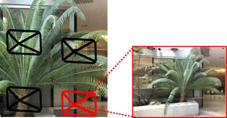
(b) Few View Synthesis

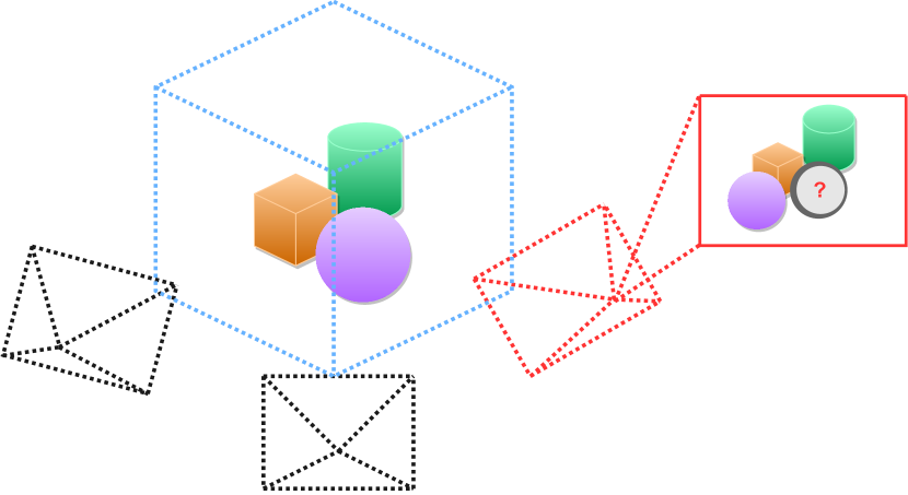
(c) Sparse View Synthesis

Figure 1: Different view synthesis operating modes, with varying numbers of views and varying baselines between views. In each case the black cameras are reference views and the red camera is the target view. Note that with few views and a wide baseline, occluded regions appear in the rendered scene which are visible in only 1 or none of the reference views.

1 Introduction

Novel view synthesis (NVS) is the problem of generating new camera viewpoints of a scene, given a fixed set of views of the same scene. Most modern NVS methods approach the problem as that of learning a generative model for the scene, conditioned on the camera pose. Key challenges with current NVS approaches are inferring the scene’s 3D structure given a restricted set of reference views, which are not necessarily coplanar with the target view. We call this the Sparse View Synthesis problem, and it raises significant challenges with the inpainting of occluded and unseen parts of the scene. This task has wide applications in image and video editing, Virtual Reality, or as a pre-processing step for other computer vision and robotics tasks. This makes novel view synthesis a key problem in modern computer vision.

Recent years have seen rapid growth in this field. Most notably, neural rendering approaches like Neural Radiance Fields (NeRF) and its advancement [Mildenhall et al.(2020)Mildenhall, Srinivasan, Tancik, Barron, Ramamoorthi, and Ng, Martin-Brualla et al.(2021)Martin-Brualla, Radwan, Sajjadi, Barron, Dosovitskiy, and Duckworth] have become very popular due to their photo-realistic results. However, these approaches tend to be very expensive, requiring a multitude of input views and a very long per-scene optimization process to obtain high-quality radiance fields. While this can be useful for tasks such a 3D object reconstruction for graphics design, it is far from practical and accessible for other applications such as live event capture.

This work aims to make neural scene reconstruction more accessible and applicable to real world scene capture. In particular we propose a method which does not require scene-specific model training, while still providing realistic results from a small sparse set of input views. We refer to this problem as Sparse View Synthesis. The key challenge is effectively recognizing and handling occluded areas, which were not observed from the small number of training views, while keeping rendering efficient. This necessitates a greater focus on generalization and extrapolation and pure synthesis, as opposed to the data aggregation of traditional radiance field models.

Some methods have approached this generalisation problem by reconstructing geometry priors. Indeed models like [Chibane et al.(2021)Chibane, Bansal, Lazova, and Pons-Moll, Chen et al.(2021)Chen, Xu, Zhao, Zhang, Xiang, Yu, and Su] attempt to replicate classic multi-view stereo behaviour using deep learning techniques. However, these approaches have focused on narrow baseline extrapolation, where occlusions are limited.

To be able to deal with occlusions and artefacts sensibly, we unify adversarial training with radiance field models (fig. 1). The adversarial training paradigm was first introduced as Generative Adversarial Networks [Goodfellow et al.(2014)Goodfellow, Pouget-Abadie, Mirza, Xu, Warde-Farley, Ozair, Courville, and Bengio]. This was designed to help enrich the output variability of generative models, while dealing with artefacts in a realistic way. In the domain of neural radiance fields, this has the potential to ensure realistic extrapolation in unobserved regions. We have made our code publicly available.

2 Background

Classical approaches to novel view synthesis (also known as Image-based rendering (IBR) [McMillan and Bishop(1995), Debevec et al.(1998)Debevec, Yu, and Borshukov, Chaurasia et al.(2013)Chaurasia, Duchene, Sorkine-Hornung, and Drettakis]) have typically relied on restrictive intermediate representations of geometry. These range from multi-layer representations like Plane Sweep Volumes [Flynn et al.(2016)Flynn, Neulander, Philbin, and Snavely, Xu et al.(2019)Xu, Bi, Sunkavalli, Hadap, Su, and Ra], Multi-Plane Images (MPI) [Zhou et al.(2018)Zhou, Tucker, Flynn, Fyffe, and Snavely, Flynn et al.(2019)Flynn, Broxton, Debevec, DuVall, Fyffe, Overbeck, Snavely, and Tucker], or Layered Depth Images (LDIs) [Shade et al.(1998)Shade, Gortler, He, and Szeliski, Shih et al.(2020)Shih, Su, Kopf, and Huang] to more complex voxel grids [Sitzmann et al.(2019)Sitzmann, Thies, Heide, Nießner, Wetzstein, and Zollhöfer, Shi et al.(2021)Shi, Li, and Yu] and 3D point clouds [Wiles et al.(2020)Wiles, Gkioxari, Szeliski, and Johnson, Xu et al.(2022)Xu, Xu, Philip, Bi, Shu, Sunkavalli, and Neumann].

More recently, NeRF [Mildenhall et al.(2020)Mildenhall, Srinivasan, Tancik, Barron, Ramamoorthi, and Ng] proposed an entirely neural scene representation, where a Multi-Layer Perceptron (MLP) parameterises a volumetric function which maps position and viewing direction to density and colour. Unfortunately, in it’s original form NeRF is very costly to run and has to be optimised per scene, which prevents it from being useful in many important applications. Subsequent approaches [Martin-Brualla et al.(2021)Martin-Brualla, Radwan, Sajjadi, Barron, Dosovitskiy, and Duckworth, Barron et al.(2021)Barron, Mildenhall, Tancik, Hedman, Martin-Brualla, and Srinivasan, Srinivasan et al.(2021)Srinivasan, Deng, Zhang, Tancik, Mildenhall, and Barron] have tried to loosen these constraints or improve performance [Hu et al.(2022)Hu, Liu, Chen, Shen, and Jia]. Despite this, all these approaches struggle to generalise across scenes, require dense input images, and are very costly to run. In particular recent works have focused on introducing additional data augmentation [Chen et al.(2022)Chen, Wang, Fan, and Wang] and regularisation systems [Kim et al.(2022)Kim, Seo, and Han, Rebain et al.(2022)Rebain, Matthews, Yi, Lagun, and Tagliasacchi, Niemeyer et al.(2022)Niemeyer, Barron, Mildenhall, Sajjadi, Geiger, and Radwan, Deng et al.(2022)Deng, Liu, Zhu, and Ramanan] to reduce the number of viewpoints required to build a scene-specific NeRF model.

To overcome the limitations of the scene-specific implicit representation, some approaches have attempted to combine the geometry learning strengths of IBR approaches with the power of neural rendering techniques. IBRNet [Wang et al.(2021)Wang, Wang, Genova, Srinivasan, Zhou, Barron, Martin-Brualla, Snavely, and Funkhouser] aggregates 2D feature information from source views along a given ray to compute its final colour. SRF [Chibane et al.(2021)Chibane, Bansal, Lazova, and Pons-Moll] emulates classical stereo matching techniques by learning an ensemble of pair-wise similarities. But the results are very blurry, cannot handle specularities, and the model is very expensive to run. PixelNeRF [Yu et al.(2021)Yu, Ye, Tancik, and Kanazawa] manages to generalise to new scenes using as few as one input image and no explicit geometry-aware 3D structures. However, it tends to overfit to the training set, failing to generalise well.On the other hand, MVSNeRF [Chen et al.(2021)Chen, Xu, Zhao, Zhang, Xiang, Yu, and Su] reconstructs an encoding volume based on a 3D feature Plane Sweep Volume [Flynn et al.(2016)Flynn, Neulander, Philbin, and Snavely]. This model works on only three input images and is generalisable to different scenes. Further developments were made based on geometric constraints [Johari et al.(2022)Johari, Lepoittevin, and Fleuret] and recurrent aggregation [Zhang et al.(2022)Zhang, Bi, Sunkavalli, Su, and Xu]. However, in all these systems only the scene content visible from the reference view is well reconstructed. The outputs contain significant artefacts in challenging or occluded regions which require further fine-tuning per scene. These techniques also lack any mechanism to generate image content in areas which are occluded in all inputs. This becomes a significant problem in Sparse View Synthesis problems, where the target view is not closely aligned with the reference view.

With the development of Generative Adversarial Networks (GANs) [Goodfellow et al.(2014)Goodfellow, Pouget-Abadie, Mirza, Xu, Warde-Farley, Ozair, Courville, and Bengio], it has become possible to generate novel photo-realistic content [Karras et al.(2019)Karras, Laine, and Aila, Karras et al.(2020)Karras, Laine, Aittala, Hellsten, Lehtinen, and Aila, Choi et al.(2018)Choi, Choi, Kim, Ha, Kim, and Choo, Choi et al.(2020)Choi, Uh, Yoo, and Ha]. Several works have applied adversarial methods to the controllable novel view synthesis of objects. HoloGAN [Nguyen-Phuoc et al.(2019)Nguyen-Phuoc, Li, Theis, Richardt, and Yang] learns object representations extracting 3D features from single natural images and disentangles shape and appearance. GRAF [Schwarz et al.(2020)Schwarz, Liao, Niemeyer, and Geiger] achieves disentanglement of object properties while not requiring 3D supervision. All single-view methods base their 3D representations on a single 2D image, which suffer from single-view spatial ambiguities. Nanbo et al [Nanbo et al.(2020)Nanbo, Eastwood, and Fisher] address this by trying to composite multi-object scenes leveraging multiple views. GIRAFFE [Niemeyer and Geiger(2021)] incorporates compositional 3D scene structure to the model to handle multi-object scenes. Pix2NeRF [Cai et al.(2022)Cai, Obukhov, Dai, and Van Gool] trained a generator system to produce random NeRF volumes which could then be combined with a decoder for GAN inversion. GNeRF [Meng et al.(2021)Meng, Chen, Luo, Wu, Su, Xu, He, and Yu] uses adversarial training to reconstruct NeRFs with unknown camera poses. pi-GAN [Chan et al.(2021)Chan, Monteiro, Kellnhofer, Wu, and Wetzstein] models partial single objects using periodic activation functions. All of these models aim to disentangle image composition for scene editing, or are limited to simple scenes comprised of one or a few simple objects. DeVris et al [DeVries et al.(2021)DeVries, Bautista, Srivastava, Taylor, and Susskind] decompose complex scenes in many local specialised Radiance Fields. This requires additional depth information and extremely expensive training. Our method on the other hand leverages adversarial training to achieve photo-realistic image generation of unconstrained occluded areas in Sparse View Synthesis.

3 Approach

We propose a pipeline based on a Plane Sweep Volume [Flynn et al.(2016)Flynn, Neulander, Philbin, and Snavely] neural encoding following MVSNeRF [Chen et al.(2021)Chen, Xu, Zhao, Zhang, Xiang, Yu, and Su]. From this volume we sample random patches using radiance fields [Mildenhall et al.(2020)Mildenhall, Srinivasan, Tancik, Barron, Ramamoorthi, and Ng] which are supervised by an adversarial loss. As opposed to [Mildenhall et al.(2020)Mildenhall, Srinivasan, Tancik, Barron, Ramamoorthi, and Ng], we don’t require a dense set of input images. We aim to learn a general model that can be applied to new unseen scenes without fine-tuning. Our model also aims to handle significant occlusions due to large baseline changes from sparse input viewpoints. In particular, we train a generalisable adversarial framework for radiance fields. An overall visualisation of our proposed model can be seen in Figure 2.

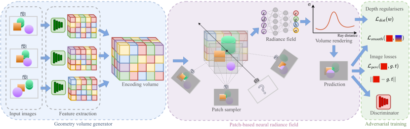
Figure 2: Model overview.

Given some sparse input images our model reconstructs an embedded neural volume which allows the model to reason about the implicit geometry of a scene. We use ray marching to sample from this volume and render a new point of view. We leverage adversarial training to help provide plausible rendering for large dis-occlusions and artefacts that arise from the large baseline changes. The following sections will detail each of these elements of our approach in turn.

3.1 Geometry volume generator

As the initial encoder for our generator, we use a 3D CNN encoding volume [Chen et al.(2021)Chen, Xu, Zhao, Zhang, Xiang, Yu, and Su] which integrates 2D CNN features of the input images. This allows the network to extract correlations between images, which can then be used to reason about geometry. The focus on image correlations as a mechanism for geometry extraction helps the network generalise to previously unseen scenes. The encoding volume is created at the reference view by warping multiple sweeping planes of source view features. This is in contrast to techniques like Deep Stereo [Flynn et al.(2016)Flynn, Neulander, Philbin, and Snavely], which perform plane sweeps using the raw colour pixels to produce their correlation volume.

To construct this volume, we first extract the deep features $\{\mathbf{F}_{i}\mid\mathbf{F}_{i}\in\mathbb{R}^{\frac{H}{4}\times\frac{W}{4}\times C}\}_{i=1}^{N}$ of the N input images $\{\mathbf{I}_{i}\mid\mathbf{I}_{i}\in\mathbb{R}^{H\times W\times 3}\}_{i=1}^{N}$ using a deep 2D convolutional network $\mathbf{F}_{i}=E(\mathbf{I}_{i}|\mathbf{w}_{E})$. This network consists of downsampling convolutional layers, batch-normalization and ReLU activation layers. For efficiency and generality, the feature encoding network is shared across all views [Yao et al.(2018)Yao, Luo, Li, Fang, and Quan].

Next we must align each feature map $\{\mathbf{F}_{i}\}$ to the reference view at multiple depths to encode the plane sweep volume. To achieve this, a homography $\mathcal{H}_{i}\left(d\right)$ is computed for each view at each depth. Given the camera parameters $\{\mathbf{K}_{i},\mathbf{R}_{i},\mathbf{t}_{i}\}$ (intrinsics, rotation and translation) for camera $i$ the homography is defined as

$$\mathcal{H}_{i}\left(d\right)=\mathbf{K}_{i}\cdot\mathbf{R}_{i}\cdot\left(\mathbf{I}+\frac{\left(\mathbf{t}_{ref}-\mathbf{t}_{i}\right)\cdot\mathbf{n}_{ref}^{T}}{d}\right)\cdot\mathbf{R}_{ref}^{T}\cdot\mathbf{K}_{ref}^{T}$$ (1)

where $\mathbf{I}$ is the $3\times 3$ identity matrix, $\mathbf{n}_{ref}$ the principle axis of the reference camera, and $d$ is the depth which the images are being warped to. This operation is differentiable, which allows for end-to-end training of the feature encoding network weights $\mathbf{w}_{E}$ based on the downstream reconstruction losses.

Applying this homography to the feature maps gives us the warped feature sweep volumes

$$\mathbf{V}_{i}=\{\mathbf{F}_{i}\cdot\mathcal{H}_{i}\left(d\right)\mid\forall d=1,...,D\}.$$ (2)

Then, a cost volume $\mathbf{C}$ is created by aggregating all the warped feature sweep volumes, which encode appearance variations across views. To do this, a variance based cost metric is used, as it allows to use an arbitrary number of input views,

$$\mathbf{C}=Var\left(\mathbf{V}_{i}\right)=\frac{\sum_{i=1}^{N}\left(\mathbf{V}_{i}-\overline{\mathbf{V}}_{i}\right)^{2}}{N}.$$ (3)

This cost volume is then processed using a 3D CNN UNet-like network [Ronneberger et al.(2015)Ronneberger, Fischer, and Brox]. This includes downsampling and upsampling layers with skip connections, to propagate scene appearance information. The output of this network is the neural embedding volume $\mathbf{E}=V(\mathbf{C}|\mathbf{w}_{V})$. This embedding volume represents the feature correlations from the point of view of the reference frame’s plane sweep volume. The structure of this volume is consistent across any arrangement of input viewpoints, and even any number of input views. This allows the system to generalize to new scene arrangements.

3.2 Volume rendering

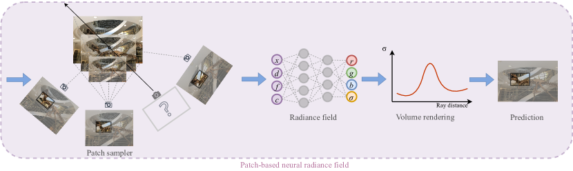
Figure 3: Volume rendering pipeline

We next use a neural radiance MLP with parameters $\mathbf{w}_{\Theta}$ to decode the embedding volume into volume density and view-dependent radiance (colour). Given a 3D point $x$, and a viewing direction $d$, we optimise a network $F_{\Theta}$ to regress the density $\sigma$ and colour $r$ from the volume $\mathbf{E}$ at that point $x$. To allow the correlations and structures in $\mathbf{E}$ to be mapped back to the original scene albedo, we use the pixel colour of the original image inputs $\mathbf{I}$ as additional conditioning information.

$$F_{\Theta}\colon\left(x,d,\mathbf{E},\mathbf{I}|\mathbf{w}_{\Theta}\right)\mapsto\left(\sigma_{x,d},r_{x,d}\right)$$ (4)

We use differentiable ray marching to regress the colour of reference image pixels. This is done by projecting (“marching”) a ray through a pixel $p$ in the reference image $\mathbf{I}_{ref}$. We can use the neural radiance network to obtain the radiance $r_{\gamma}$ and density $\sigma_{\gamma}$ at regular intervals $\gamma\in[1..\inf]$ along this ray via

$$\left(\sigma_{\gamma},r_{\gamma}\right)=F_{\Theta}\left(\mathbf{t}_{ref}+\gamma\hat{d},\hat{d},\mathbf{E},\mathbf{I}|\mathbf{w}_{\Theta}\right)$$ (5)

where $\hat{d}=\mathbf{R}_{ref}^{T}\cdot\mathbf{K}_{ref}^{T}p$. We can use these regular samples from $F_{\Theta}$ to obtain the predicted colour of the pixel $R(p)$ via volume rendering equation [Kajiya and Herzen(1984)]:

$$R(p) =\sum_{\gamma}\tau_{\gamma}\left(1-exp\left(-\sigma_{\gamma}\right)\right)r_{\gamma}$$ (6)

$$\tau_{\gamma} =exp\left(-\sum_{j=1}^{\gamma-1}\sigma_{j}\right)$$ (7)

where $\tau_{\gamma}$ is the transmittance at sample $\gamma$, which represents the probability that the ray travels up to $\gamma$ without hitting another particle.

It is intuitive that the proposed approach will be able to predict density based on the consistency of feature representations between views. We can even see how analysing exactly which views correlate well for a given point can provide hints about occlusions, and guidance for albedo lookup. However, there is no simple mechanism to distinguish a region which has low correlation due to being empty, and one with low correlation due to being occluded in all views. The prevalence of these fully occluded regions grows drastically as the number of input views is reduced, and leads traditional radiance field models to produce reconstructions full of unrealistic holes.

3.3 Adversarial training

To combat this, we couple the above Generator network with a Discriminator network and undertake adversarial training. This makes it possible to enforce realism in unobserved regions. However, effective adversarial training requires spatial structure in the generated output, therefore we use a patch based neural generator function based on equation 6. The use of a patch based generator serves two purposes. Firstly, it exponentially increases the number of possible training samples, ensuring that the discriminator is not able to memorize the training dataset. Secondly it greatly improves training efficiency as it can be expensive to repeatedly render entire images via the Neural Radiance Field.

Following Schwarz et al [Schwarz et al.(2020)Schwarz, Liao, Niemeyer, and Geiger], we generate a variable patch that scales with training time. This allows for a variable receptive field. The patch $\mathbf{P}_{p}$ centred on pixel $p$ of size $\delta\times\delta$ is defined as

$$\mathbf{P}\left(p,s\right)=\left\{\left(si+p_{x},sj+p_{y}\right)\mid i,j\in\left\{-\frac{\delta}{2},...,\frac{\delta}{2}\right\}\right\}$$ (8)

where $s$ is the scale that controls the active field of the patch. The scale exponentially decays during the training process, allowing our convolutional discriminator to learn independently of the image resolution.

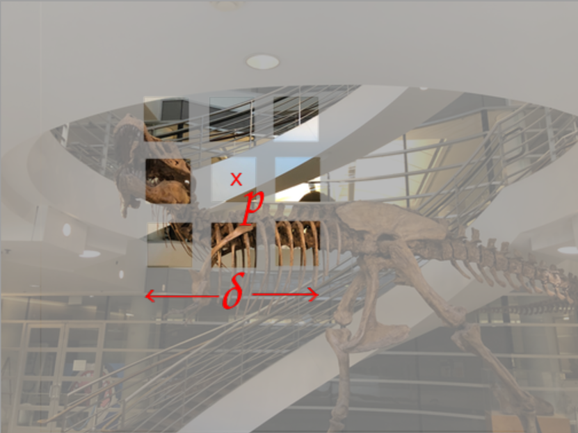
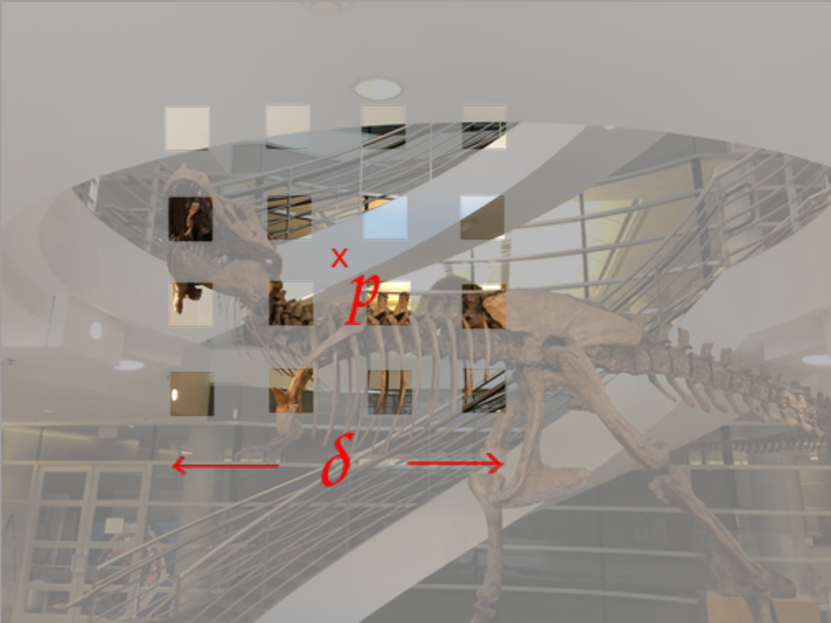
Figure 4: Patches. An illustration of the varying patch scale over the course of training.

Given the ground truth patch $\mathbf{P}_{p}^{*}$ for the target view, we compute the $L_{1}$ loss between a randomly selected real and target patch

$$\mathcal{L}_{rec}=||\mathbf{P}_{p}-\mathbf{P}_{p}^{*}||\text{ where }p\sim\mathcal{U}([0,0],[W,H]).$$ (9)

This $L_{1}$ loss is effective at enforcing low-frequency correctness in the output. However, it can lead to overly-blurred results and difficulty recovering high-frequency structures. We therefore follow an LSGAN [Mao et al.(2017)Mao, Li, Xie, Lau, Wang, and Smolley] approach and augment this with a convolutional PatchGAN [Isola et al.(2017)Isola, Zhu, Zhou, and Efros] discriminator network $D_{\Phi}$ with parameters $\mathbf{w}_{\Phi}$.

The discriminator network takes patches as input, and is trained to classify input patches from the ground truth and from the generator as real or fake respectively. As such the discriminator loss is defined as

$$\mathcal{L}_{D}=||1-D_{\Phi}\left(\mathbf{P}_{p}^{*}\right)||_{2}^{2}+||D_{\Phi}\left(\mathbf{P}_{p}\right)||_{2}^{2}\text{ where }p\sim\mathcal{U}([0,0],[W,H]).$$ (10)

Finally, we can use the PatchGAN discriminator’s loss to also create an adversarial loss which constrains the generator network

$$\mathcal{L}_{G}=\lambda||1-D_{\Phi}\left(\mathbf{P}_{p}\right)||_{2}^{2}\text{ where }p\sim\mathcal{U}([0,0],[W,H]).$$ (11)

where $\lambda$ is a weighting factor. This adversarial loss encourages the generator to produce more realistic outputs which are able to fool the discriminator. Importantly, any holes in the reconstruction due to occlusions will provide obvious clues for the discriminator. Therefore the generator can only succeed in its task if the holes are filled with hallucinated photo-realistic content.

We should re-iterate that this entire pipeline is fully differentiable. This includes the discriminator, the patch based volumetric rendering, the radiance field estimation, the feature correlation computation, the homographic plane-sweep warping and the input image feature lookup. As such, our adversarial loss $\mathcal{L}_{G}$ is able to constrain all the learnable parameters $\mathbf{w}_{E},\mathbf{w}_{V},\mathbf{w}_{\Theta}$ apart from those in the discriminator $\mathbf{w}_{\Phi}$ which are optimised based on $\mathcal{L}_{D}$. These two optimizations are performed using separate Adam optimisers [Kingma and Ba(2014)] which are alternated.

3.4 Depth regularisation

Because Sparse View Synthesis is an ill-defined problem, we found that the predicted depth images were extremely noisy, if not completely nonsensical. To be able to reconstruct a well defined scene geometry, the predicted depth needs to be coherent with the image. We approach this issue by adding two depth regularisers.

3.4.1 Edge-aware depth smoothness

Firstly, we introduce a depth smoothness loss to encourage the network to generate continuous surfaces, similar to monocular depth estimation approaches [Godard et al.(2017)Godard, Mac Aodha, and Brostow]. As depth discontinuities usually happen at colour edges [Heise et al.(2013)Heise, Klose, Jensen, and Knoll], the depth smoothness is weighted with the colour image gradients $\partial I$.

$$\mathcal{L}_{smooth}\left(d\right)=\frac{1}{N}\sum_{i,j}\left[\left|\partial_{x}d_{ij}\right|\mathrm{e}^{-||\partial_{x}I_{ij}||}+\left|\partial_{y}d_{ij}\right|\mathrm{e}^{-||\partial_{y}I_{ij}||}\right]$$ (12)

where $d_{i,j}$ is the predicted depth at pixel $(i,j)$, and $I_{i,j}$ the respective colour value.

3.4.2 Distortion loss

In addition to smooth surfaces, we also want to get rid of other potential artefacts like “floaters” (small disconnected regions of occupied space that look fine from the input views, but wouldn’t be coherent if seen from another view), and “background collapse” (far surfaces modeled as semi-transparent clouds of dense content in the foreground). NeRF-based models [Mildenhall et al.(2020)Mildenhall, Srinivasan, Tancik, Barron, Ramamoorthi, and Ng] try to achieve this by adding Gaussian noise to the output $\sigma$ values during optimisation. But this does not eliminate all geometry artefacts, and reduces the reconstruction quality. Instead, we follow Barron et al [Barron et al.(2022)Barron, Mildenhall, Verbin, Srinivasan, and Hedman] and include a distortion loss in our regularisation.

$$\mathcal{L}_{dist}\left(\mathbf{w}\right) =\sum_{i,j}\mathrm{w}_{i}\mathrm{w}_{j}+\frac{1}{3}\sum_{i}\mathrm{w}^{2}_{i}$$ (13)

$$\mathrm{w}_{i} =\tau_{i}\left(1-exp\left(-\sigma_{i}\right)\right)$$ (14)

where $\mathrm{w}_{i}$ are the alpha compositing weights at ray sample $i$, derived from equation 6. This regulariser minimises the weighted distances between all pairs of ray points, and the weighted size of each individual point. This helps the distribution function of the density along the rays approximates a delta function. Finally, we combine all the generator losses and regularisers with an LPIPS [Zhang et al.(2018)Zhang, Isola, Efros, Shechtman, and Wang] perceptual loss. Our total loss is as follows:

$$\mathcal{L}_{total}=\frac{1}{2}\mathcal{L}_{D}+\mathcal{L}_{G}+\lambda_{rec}\mathcal{L}_{rec}+\mathcal{L}_{perc}+\lambda_{smooth}\mathcal{L}_{smooth}+\lambda_{dist}\mathcal{L}_{dist}$$ (15)

where we chose $\lambda_{rec}=20,\lambda_{smooth}=0.4,\lambda_{dist}=0.001$ for our experiments.

4 Experimental setup

For training we are using two different commonly used datasets, DTU [Jensen et al.(2014)Jensen, Dahl, Vogiatzis, Tola, and Aanæs] and Forward-Facing (LLFF) data [Mildenhall et al.(2019)Mildenhall, Srinivasan, Ortiz-Cayon, Kalantari, Ramamoorthi, Ng, and Kar]. The DTU dataset consists of a variety of scenes and objects taken in a lab setup. We follow the same training approach in related papers [Yu et al.(2021)Yu, Ye, Tancik, and Kanazawa, Chen et al.(2021)Chen, Xu, Zhao, Zhang, Xiang, Yu, and Su], and split the dataset into 88 training scenes and 16 testing scenes, using an image resolution of 512$\times$640. The Forward-Facing dataset consists of handheld phone captures taken in a 2D grid. We split the dataset into 35 training sets and 8 for testing in the same scenes used for NeRF. Because we focus on the sparse view synthesis problem, models are trained on 3 input views per scene.

4.1 Baseline models

We compare our method against the current state-of-the-art neural rendering methods for Sparse View Synthesis. All methods are trained over LLFF and DTU using three input images. We evaluate IBRNet [Wang et al.(2021)Wang, Wang, Genova, Srinivasan, Zhou, Barron, Martin-Brualla, Snavely, and Funkhouser], MVSNeRF [Chen et al.(2021)Chen, Xu, Zhao, Zhang, Xiang, Yu, and Su] and our method over long baseline movements. We weren’t able to train GeoNeRF [Johari et al.(2022)Johari, Lepoittevin, and Fleuret] as the code hasn’t been released yet, and the results in their paper are for a much easier problem.

4.2 Evaluation of accuracy

For the purpose of quantifying how well our model performs, we make use of several popular metrics that measure different characteristics of an image. To measure image quality, we use Peak Signal-To-Noise Ratio (PSNR) [Huynh-Thu and Ghanbari(2008)] and Structural SIMilarity (SSIM) [Wang, Zhou et al.(2004)Wang, Zhou, Bovik, Sheikh, and Simoncelli] index. PSNR shows the overall pixel consistency, while SSIM measures the coherence of local structures. These metrics assume pixel-wise independence, which may assign favourable scores to perceptually inaccurate results. For this reason, we also include the use of a Learned Perceptual Image Patch Similarity (LPIPS) [Zhang et al.(2018)Zhang, Isola, Efros, Shechtman, and Wang] metric, which aims to capture human perception using deep features.

Table 1: Quantitative evaluation. We evaluate our model over the DTU and Forward Facing datasets. Bold is best result, italic is second best.

Model	Experiment	DTU			Forward facing
		PSNR$\uparrow$	SSIM$\uparrow$	LPIPS$\downarrow$	PSNR$\uparrow$	SSIM$\uparrow$	LPIPS$\downarrow$
RegNeRF* [Niemeyer et al.(2022)Niemeyer, Barron, Mildenhall, Sajjadi, Geiger, and Radwan]	Optimised	18.89	0.745	0.190	19.08	0.587	0.336
IBRNet [Wang et al.(2021)Wang, Wang, Genova, Srinivasan, Zhou, Barron, Martin-Brualla, Snavely, and Funkhouser]	Unseen	12.71	0.4772	0.5678	16.40	0.5230	0.4986
MVSNeRF [Chen et al.(2021)Chen, Xu, Zhao, Zhang, Xiang, Yu, and Su]		18.92	0.6831	0.2580	16.98	0.5839	0.3853
Ours		19.03	0.6929	0.2066	16.55	0.5534	0.3441

From table 1 we can see that our proposed approach performs similarly to RegNeRF in terms of accuracy. This is despite the fact that RegNeRF is trained in a scene specific regime, while our approach is trained on unrelated scenes, then applied to a completely unknown scene at test time.

Ref. view 1

Ref. view 2

GT Target

Pred. Target

Pred. Depth

Figure 5: Example predictions for the DTU (top) and Forward Facing (bottom) datasets.

When comparing our technique against the other scene agnostic state-of-the-art approaches (IBRNet and MVSNeRF) under the Sparse View Synthesis evaluation protocol, we note that the simplistic PSNR and SSIM accuracy measures are relatively similar. However, drastic improvements are seen in the LPIPS metric over previous work ranging from a 15% to 60% improvement in the perceptual accuracy of the reconstructed scene. It is interesting to note that our approach performs especially well on the more challenging DTU dataset. Qualitative examples for both datasets are shown in figure 5. For additional examples please see the supplementary material.

Table 2: Ablation study. We study the effect of each addition to the model on the Forward facing dataset. Bold is best result, italic is second best.

Depth Smooth	Distortion	Adversarial	PSNR$\uparrow$	SSIM$\uparrow$	LPIPS$\downarrow$
$\times$	$\times$	$\times$	16.11	0.5318	0.4791
$\checked$	$\times$	$\times$	16.14	0.5361	0.4709
$\checked$	$\checked$	$\times$	16.10	0.5419	0.4611
$\checked$	$\checked$	$\checked$	16.55	0.5534	0.3441

4.3 Ablation study

In table 2 we undertake an ablation study on the Forward Facing dataset. The depth smoothing loss makes a small but noticable difference across all metrics. It is interesting to note that the distortion loss leads to a marginal decrease in the PSNR and SSIM metrics. However, it provides a more significant improvement in terms of LPIPS. This is expected, as the distortion loss slightly limits the flexibility of the volumetric rendering by preventing “smearing” the scene across depths. However, this in turn removes floating blob artifacts and blurred scene depth when viewed from distant viewpoints. These artifacts have a significant impact in the overall perceptual quality of the rendered image, and are vital for possible human-centric applications.

The final adversarial loss leads to significant improvements across all metrics, with the largest gains once again being with the LPIPS score. This demonstrates that the integration of adversarial learning is vital for producing plausible renders for Sparse View Synthesis.

5 Conclusions

In this paper we have proposed the Sparse View Synthesis problem. This is a view synthesis problem where the number of reference views is limited, and the baseline between target and reference view is significant. This is a common scenario in live event capture, virtual reality and similar domains.

This imposes a number of challenges which are not present in the standard novel view synthesis problem setup. Most notably the fact that large portions of the target view may be occluded or otherwise not visible within the reference views. In this case there is no mechanism for a standard radiance field model to appropriately fill the gap.

Therefore we proposed an algorithm which unified generative adversarial learning techniques with traditional radiance field modelling. This encouraged the system to inpaint unobserved regions with plausible scene completions. This led to perceptual quality improvements of up to 60% compared to existing radiance field models.

Nonetheless, there is still some way to go to achieve full extreme Sparse View Synthesis. Although GANs produce good results at generating new content, they suffer from the classic training instability, which makes the model harder to train. In addition, the difficulty of the problem means the complexity of the solution increases. As we handle extreme baseline movements, this creates an ill-posed problem where sometimes the network doesn’t differentiate between empty or occluded space. Thus, in areas viewed by only one of the source views, the reconstruction can lack fidelity. In future work it may be possible to resolve this by re-weighting the generative losses in different regions based on visibility. Regardless, the proposed approach is a major step towards achieving more extreme and sparse renderings.

In future work, it would be interesting to explore the integration of alternative generative modelling techniques with radiance field models. In particular, if the radiance field is able to recognise areas in which it is uncertain, diffusion networks could inpaint these regions directly.

Acknowledgements.

This work was partially supported by the British Broadcasting Corporation (BBC) and the Engineering and Physical Sciences Research Council’s (EPSRC) industrial CASE project “Generating virtual camera views with generative networks” (voucher number 19000033).

Ref. view 1
Ref. view 2
MVSNeRF[chen2021]
Ours
Ground Truth
Depth (Ours)

Figure 6: Example predictions from the DTU dataset. Each column shows a different scene predicted under the Sparse View Synthesis evaluation protocol. Note that state of the art [Chen et al.(2021)Chen, Xu, Zhao, Zhang, Xiang, Yu, and Su] predictions exhibit fuzziness or “smearing” around object boundaries where occlusions occur. In contrast our approach provides sharper edges as it realistically fills unobserved regions.

Ref. view 1
Ref. view 2
MVSNeRF[Chen et al.(2021)Chen, Xu, Zhao, Zhang, Xiang, Yu, and Su]
Ours
Ground Truth
Depth (us)

Figure 7: Example predictions from the LLFF dataset. Again we can observe “smearing” artifacts in the state-of-the-art predictions, especially along the image borders. Additionally, we can observe “halo” or “duplicated boundary” artifacts in some of the state-of-the-art scenes such as the rightmost two columns. These perceptually jarring artifacts are easily detected by our adversarial discriminator, and so they do not occur in the predictions for our approach.

References

- [Barron et al.(2021)Barron, Mildenhall, Tancik, Hedman, Martin-Brualla, and Srinivasan] Jonathan T. Barron, Ben Mildenhall, Matthew Tancik, Peter Hedman, Ricardo Martin-Brualla, and Pratul P. Srinivasan. Mip-NeRF: A Multiscale Representation for Anti-Aliasing Neural Radiance Fields. ICCV, 2021.
- [Barron et al.(2022)Barron, Mildenhall, Verbin, Srinivasan, and Hedman] Jonathan T. Barron, Ben Mildenhall, Dor Verbin, Pratul P. Srinivasan, and Peter Hedman. Mip-NeRF 360: Unbounded Anti-Aliased Neural Radiance Fields. In Proceedings of the IEEE/CVF Conference on Computer Vision and Pattern Recognition, 2022.
- [Cai et al.(2022)Cai, Obukhov, Dai, and Van Gool] Shengqu Cai, Anton Obukhov, Dengxin Dai, and Luc Van Gool. Pix2NeRF: Unsupervised Conditional $\pi$-GAN for Single Image to Neural Radiance Fields Translation. In IEEE/CVF Conference on Computer Vision and Pattern Recognition (CVPR), 2022.
- [Chan et al.(2021)Chan, Monteiro, Kellnhofer, Wu, and Wetzstein] Eric R. Chan, Marco Monteiro, Petr Kellnhofer, Jiajun Wu, and Gordon Wetzstein. Pi-GAN: Periodic Implicit Generative Adversarial Networks for 3D-Aware Image Synthesis. In 2021 IEEE/CVF Conference on Computer Vision and Pattern Recognition (CVPR), June 2021.
- [Chaurasia et al.(2013)Chaurasia, Duchene, Sorkine-Hornung, and Drettakis] Gaurav Chaurasia, Sylvain Duchene, Olga Sorkine-Hornung, and George Drettakis. Depth synthesis and local warps for plausible image-based navigation. ACM Transactions on Graphics, June 2013.
- [Chen et al.(2021)Chen, Xu, Zhao, Zhang, Xiang, Yu, and Su] Anpei Chen, Zexiang Xu, Fuqiang Zhao, Xiaoshuai Zhang, Fanbo Xiang, Jingyi Yu, and Hao Su. MVSNeRF: Fast Generalizable Radiance Field Reconstruction from Multi-View Stereo. Proceedings of the IEEE/CVF International Conference on Computer Vision, 2021.
- [Chen et al.(2022)Chen, Wang, Fan, and Wang] Tianlong Chen, Peihao Wang, Zhiwen Fan, and Zhangyang Wang. Aug-NeRF: Training Stronger Neural Radiance Fields With Triple-Level Physically-Grounded Augmentations. In Proceedings of the IEEE/CVF Conference on Computer Vision and Pattern Recognition, 2022.
- [Chibane et al.(2021)Chibane, Bansal, Lazova, and Pons-Moll] Julian Chibane, Aayush Bansal, Verica Lazova, and Gerard Pons-Moll. Stereo Radiance Fields (SRF): Learning View Synthesis for Sparse Views of Novel Scenes. In 2021 IEEE/CVF Conference on Computer Vision and Pattern Recognition (CVPR), June 2021.
- [Choi et al.(2018)Choi, Choi, Kim, Ha, Kim, and Choo] Yunjey Choi, Minje Choi, Munyoung Kim, Jung-Woo Ha, Sunghun Kim, and Jaegul Choo. StarGAN: Unified Generative Adversarial Networks for Multi-domain Image-to-Image Translation. In 2018 IEEE/CVF Conference on Computer Vision and Pattern Recognition, June 2018.
- [Choi et al.(2020)Choi, Uh, Yoo, and Ha] Yunjey Choi, Youngjung Uh, Jaejun Yoo, and Jung-Woo Ha. StarGAN v2: Diverse Image Synthesis for Multiple Domains. In 2020 IEEE/CVF Conference on Computer Vision and Pattern Recognition (CVPR), June 2020.
- [Debevec et al.(1998)Debevec, Yu, and Borshukov] Paul Debevec, Yizhou Yu, and George Borshukov. Efficient View-Dependent Image-Based Rendering with Projective Texture-Mapping. In Rendering Techniques ’98. 1998.
- [Deng et al.(2022)Deng, Liu, Zhu, and Ramanan] Kangle Deng, Andrew Liu, Jun-Yan Zhu, and Deva Ramanan. Depth-Supervised NeRF: Fewer Views and Faster Training for Free. In Proceedings of the IEEE/CVF Conference on Computer Vision and Pattern Recognition, 2022.
- [DeVries et al.(2021)DeVries, Bautista, Srivastava, Taylor, and Susskind] Terrance DeVries, Miguel Angel Bautista, Nitish Srivastava, Graham W. Taylor, and Joshua M. Susskind. Unconstrained Scene Generation with Locally Conditioned Radiance Fields. 2021 IEEE/CVF International Conference on Computer Vision (ICCV), 2021.
- [Flynn et al.(2016)Flynn, Neulander, Philbin, and Snavely] John Flynn, Ivan Neulander, James Philbin, and Noah Snavely. DeepStereo: Learning to Predict New Views from the World’s Imagery. In 2016 IEEE Conference on Computer Vision and Pattern Recognition (CVPR), June 2016.
- [Flynn et al.(2019)Flynn, Broxton, Debevec, DuVall, Fyffe, Overbeck, Snavely, and Tucker] John Flynn, Michael Broxton, Paul Debevec, Matthew DuVall, Graham Fyffe, Ryan Overbeck, Noah Snavely, and Richard Tucker. DeepView: View Synthesis with Learned Gradient Descent. Proceedings of the IEEE Computer Society Conference on Computer Vision and Pattern Recognition, June 2019.
- [Godard et al.(2017)Godard, Mac Aodha, and Brostow] Clément Godard, Oisin Mac Aodha, and Gabriel J. Brostow. Unsupervised Monocular Depth Estimation with Left-Right Consistency. In CVPR, April 2017.
- [Goodfellow et al.(2014)Goodfellow, Pouget-Abadie, Mirza, Xu, Warde-Farley, Ozair, Courville, and Bengio] Ian J. Goodfellow, Jean Pouget-Abadie, Mehdi Mirza, Bing Xu, David Warde-Farley, Sherjil Ozair, Aaron Courville, and Yoshua Bengio. Generative adversarial nets. In Proceedings of the 27th International Conference on Neural Information Processing Systems - Volume 2, December 2014.
- [Heise et al.(2013)Heise, Klose, Jensen, and Knoll] Philipp Heise, Sebastian Klose, Brian Jensen, and Alois Knoll. PM-Huber: PatchMatch with Huber Regularization for Stereo Matching. In 2013 IEEE International Conference on Computer Vision, December 2013.
- [Hu et al.(2022)Hu, Liu, Chen, Shen, and Jia] Tao Hu, Shu Liu, Yilun Chen, Tiancheng Shen, and Jiaya Jia. EfficientNeRF Efficient Neural Radiance Fields. In Proceedings of the IEEE/CVF Conference on Computer Vision and Pattern Recognition, 2022.
- [Huynh-Thu and Ghanbari(2008)] Q. Huynh-Thu and M. Ghanbari. Scope of validity of PSNR in image/video quality assessment. Electronics Letters, 2008.
- [Isola et al.(2017)Isola, Zhu, Zhou, and Efros] Phillip Isola, Jun-Yan Zhu, Tinghui Zhou, and Alexei A. Efros. Image-to-Image Translation with Conditional Adversarial Networks. Proceedings of the IEEE/CVF Conference on Computer Vision and Pattern Recognition, 2017.
- [Jensen et al.(2014)Jensen, Dahl, Vogiatzis, Tola, and Aanæs] R. Jensen, A. Dahl, G. Vogiatzis, E. Tola, and H. Aanæs. Large Scale Multi-view Stereopsis Evaluation. In 2014 IEEE Conference on Computer Vision and Pattern Recognition, June 2014.
- [Johari et al.(2022)Johari, Lepoittevin, and Fleuret] Mohammad Mahdi Johari, Yann Lepoittevin, and François Fleuret. GeoNeRF: Generalizing NeRF With Geometry Priors. In Proceedings of the IEEE/CVF Conference on Computer Vision and Pattern Recognition, 2022.
- [Kajiya and Herzen(1984)] James T. Kajiya and Brian P. Von Herzen. Ray Tracing Volume Densities. SIGGRAPH Comput. Graph., 1984.
- [Karras et al.(2019)Karras, Laine, and Aila] Tero Karras, Samuli Laine, and Timo Aila. A Style-Based Generator Architecture for Generative Adversarial Networks. In 2019 IEEE/CVF Conference on Computer Vision and Pattern Recognition, March 2019.
- [Karras et al.(2020)Karras, Laine, Aittala, Hellsten, Lehtinen, and Aila] Tero Karras, Samuli Laine, Miika Aittala, Janne Hellsten, Jaakko Lehtinen, and Timo Aila. Analyzing and Improving the Image Quality of StyleGAN. In 2020 IEEE/CVF Conference on Computer Vision and Pattern Recognition, 2020.
- [Kim et al.(2022)Kim, Seo, and Han] Mijeong Kim, Seonguk Seo, and Bohyung Han. InfoNeRF: Ray Entropy Minimization for Few-Shot Neural Volume Rendering. In 2022 IEEE/CVF Conference on Computer Vision and Pattern Recognition (CVPR), June 2022.
- [Kingma and Ba(2014)] Diederik P. Kingma and Jimmy Ba. Adam: A Method for Stochastic Optimization. International Conference on Learning Representations, 2014.
- [Mao et al.(2017)Mao, Li, Xie, Lau, Wang, and Smolley] Xudong Mao, Qing Li, Haoran Xie, Raymond Y.K. Lau, Zhen Wang, and Stephen Paul Smolley. Least Squares Generative Adversarial Networks. In Proceedings of the IEEE International Conference on Computer Vision, December 2017.
- [Martin-Brualla et al.(2021)Martin-Brualla, Radwan, Sajjadi, Barron, Dosovitskiy, and Duckworth] Ricardo Martin-Brualla, Noha Radwan, Mehdi S. M. Sajjadi, Jonathan T. Barron, Alexey Dosovitskiy, and Daniel Duckworth. NeRF in the Wild: Neural Radiance Fields for Unconstrained Photo Collections. CVPR, 2021.
- [McMillan and Bishop(1995)] Leonard McMillan and Gary Bishop. Plenoptic modeling: An image-based rendering system. In Proceedings of the 22nd Annual Conference on Computer Graphics and Interactive Techniques - SIGGRAPH ’95, 1995.
- [Meng et al.(2021)Meng, Chen, Luo, Wu, Su, Xu, He, and Yu] Quan Meng, Anpei Chen, Haimin Luo, Minye Wu, Hao Su, Lan Xu, Xuming He, and Jingyi Yu. GNeRF: GAN-based Neural Radiance Field without Posed Camera. 2021 IEEE/CVF International Conference on Computer Vision (ICCV), 2021.
- [Mildenhall et al.(2019)Mildenhall, Srinivasan, Ortiz-Cayon, Kalantari, Ramamoorthi, Ng, and Kar] Ben Mildenhall, Pratul P. Srinivasan, Rodrigo Ortiz-Cayon, Nima Khademi Kalantari, Ravi Ramamoorthi, Ren Ng, and Abhishek Kar. Local Light Field Fusion: Practical View Synthesis with Prescriptive Sampling Guidelines. ACM Transactions on Graphics (TOG), May 2019.
- [Mildenhall et al.(2020)Mildenhall, Srinivasan, Tancik, Barron, Ramamoorthi, and Ng] Ben Mildenhall, Pratul P. Srinivasan, Matthew Tancik, Jonathan T. Barron, Ravi Ramamoorthi, and Ren Ng. NeRF: Representing Scenes as Neural Radiance Fields for View Synthesis. In ECCV, 2020.
- [Nanbo et al.(2020)Nanbo, Eastwood, and Fisher] Li Nanbo, Cian Eastwood, and Robert B. Fisher. Learning Object-Centric Representations of Multi-Object Scenes from Multiple Views. NIPS’20: Proceedings of the 34th International Conference on Neural Information Processing Systems, 2020.
- [Nguyen-Phuoc et al.(2019)Nguyen-Phuoc, Li, Theis, Richardt, and Yang] Thu Nguyen-Phuoc, Chuan Li, Lucas Theis, Christian Richardt, and Yong-Liang Yang. HoloGAN: Unsupervised learning of 3D representations from natural images. The IEEE International Conference on Computer Vision (ICCV), 2019.
- [Niemeyer and Geiger(2021)] Michael Niemeyer and Andreas Geiger. GIRAFFE: Representing Scenes as Compositional Generative Neural Feature Fields. Proc. IEEE Conf. on Computer Vision and Pattern Recognition (CVPR), 2021.
- [Niemeyer et al.(2022)Niemeyer, Barron, Mildenhall, Sajjadi, Geiger, and Radwan] Michael Niemeyer, Jonathan T. Barron, Ben Mildenhall, Mehdi S. M. Sajjadi, Andreas Geiger, and Noha Radwan. RegNeRF: Regularizing Neural Radiance Fields for View Synthesis From Sparse Inputs. In Proceedings of the IEEE/CVF Conference on Computer Vision and Pattern Recognition (CVPR), 2022.
- [Rebain et al.(2022)Rebain, Matthews, Yi, Lagun, and Tagliasacchi] Daniel Rebain, Mark Matthews, Kwang Moo Yi, Dmitry Lagun, and Andrea Tagliasacchi. LOLNeRF: Learn from One Look. In 2022 IEEE/CVF Conference on Computer Vision and Pattern Recognition (CVPR), June 2022.
- [Ronneberger et al.(2015)Ronneberger, Fischer, and Brox] Olaf Ronneberger, Philipp Fischer, and Thomas Brox. U-Net: Convolutional Networks for Biomedical Image Segmentation. In Medical Image Computing and Computer-Assisted Intervention – MICCAI, 2015.
- [Schwarz et al.(2020)Schwarz, Liao, Niemeyer, and Geiger] Katja Schwarz, Yiyi Liao, Michael Niemeyer, and Andreas Geiger. GRAF: Generative Radiance Fields for 3D-Aware Image Synthesis. In Advances in Neural Information Processing Systems (NeurIPS), 2020.
- [Shade et al.(1998)Shade, Gortler, He, and Szeliski] Jonathan Shade, Steven Gortler, Li-wei He, and Richard Szeliski. Layered depth images. In Proceedings of the 25th Annual Conference on Computer Graphics and Interactive Techniques - SIGGRAPH ’98, 1998.
- [Shi et al.(2021)Shi, Li, and Yu] Yujiao Shi, Hongdong Li, and Xin Yu. Self-Supervised Visibility Learning for Novel View Synthesis. Proceedings of the IEEE Conference on Computer Vision and Pattern Recognition, 2021.
- [Shih et al.(2020)Shih, Su, Kopf, and Huang] Meng-Li Shih, Shih-Yang Su, Johannes Kopf, and Jia-Bin Huang. 3D Photography using Context-aware Layered Depth Inpainting. IEEE Conference on Computer Vision and Pattern Recognition (CVPR), April 2020.
- [Sitzmann et al.(2019)Sitzmann, Thies, Heide, Nießner, Wetzstein, and Zollhöfer] Vincent Sitzmann, Justus Thies, Felix Heide, Matthias Nießner, Gordon Wetzstein, and Michael Zollhöfer. DeepVoxels: Learning Persistent 3D Feature Embeddings. In Proc. Computer Vision and Pattern Recognition (CVPR), IEEE, 2019.
- [Srinivasan et al.(2021)Srinivasan, Deng, Zhang, Tancik, Mildenhall, and Barron] Pratul P. Srinivasan, Boyang Deng, Xiuming Zhang, Matthew Tancik, Ben Mildenhall, and Jonathan T. Barron. NeRV: Neural Reflectance and Visibility Fields for Relighting and View Synthesis. CVPR, 2021.
- [Wang et al.(2021)Wang, Wang, Genova, Srinivasan, Zhou, Barron, Martin-Brualla, Snavely, and Funkhouser] Qianqian Wang, Zhicheng Wang, Kyle Genova, Pratul Srinivasan, Howard Zhou, Jonathan T. Barron, Ricardo Martin-Brualla, Noah Snavely, and Thomas Funkhouser. IBRNet: Learning Multi-View Image-Based Rendering. In 2021 IEEE/CVF Conference on Computer Vision and Pattern Recognition (CVPR), June 2021.
- [Wang, Zhou et al.(2004)Wang, Zhou, Bovik, Sheikh, and Simoncelli] Wang, Zhou, A. C. Bovik, H. R. Sheikh, and E. P. Simoncelli. Image quality assessment: From error visibility to structural similarity. IEEE Transactions on Image Processing, April 2004.
- [Wiles et al.(2020)Wiles, Gkioxari, Szeliski, and Johnson] Olivia Wiles, Georgia Gkioxari, Richard Szeliski, and Justin Johnson. SynSin: End-to-end View Synthesis from a Single Image. CVPR, 2020.
- [Xu et al.(2022)Xu, Xu, Philip, Bi, Shu, Sunkavalli, and Neumann] Qiangeng Xu, Zexiang Xu, Julien Philip, Sai Bi, Zhixin Shu, Kalyan Sunkavalli, and Ulrich Neumann. Point-NeRF: Point-based Neural Radiance Fields. In 2022 IEEE/CVF Conference on Computer Vision and Pattern Recognition (CVPR), June 2022.
- [Xu et al.(2019)Xu, Bi, Sunkavalli, Hadap, Su, and Ra] Zexiang Xu, Sai Bi, Kalyan Sunkavalli, Sunil Hadap, Hao Su, and Ravi Ra. Deep View Synthesis from Sparse Photometric Images. ACM Trans. Graph, 2019.
- [Yao et al.(2018)Yao, Luo, Li, Fang, and Quan] Yao Yao, Zixin Luo, Shiwei Li, Tian Fang, and Long Quan. MVSNet: Depth Inference for Unstructured Multi-view Stereo. European Conference on Computer Vision (ECCV), 2018.
- [Yu et al.(2021)Yu, Ye, Tancik, and Kanazawa] Alex Yu, Vickie Ye, Matthew Tancik, and Angjoo Kanazawa. pixelNeRF: Neural Radiance Fields From One or Few Images. In CVPR, 2021.
- [Zhang et al.(2018)Zhang, Isola, Efros, Shechtman, and Wang] Richard Zhang, Phillip Isola, Alexei A. Efros, Eli Shechtman, and Oliver Wang. The Unreasonable Effectiveness of Deep Features as a Perceptual Metric. In IEEE/CVF Conference on Computer Vision and Pattern Recognition, June 2018.
- [Zhang et al.(2022)Zhang, Bi, Sunkavalli, Su, and Xu] Xiaoshuai Zhang, Sai Bi, Kalyan Sunkavalli, Hao Su, and Zexiang Xu. NeRFusion: Fusing Radiance Fields for Large-Scale Scene Reconstruction. In Proceedings of the IEEE/CVF Conference on Computer Vision and Pattern Recognition, 2022.
- [Zhou et al.(2018)Zhou, Tucker, Flynn, Fyffe, and Snavely] Tinghui Zhou, Richard Tucker, John Flynn, Graham Fyffe, and Noah Snavely. Stereo magnification: Learning view synthesis using multiplane images. In SIGGRAPH, August 2018.