Sequential Optimization of CVaR

Abstract

This paper studies optimization of the Conditional Value at Risk (CVaR) for a discounted total-cost Markov Decision Process (MDP) with finite state and action sets. This CVaR optimization problem can be reformulated as a Robust MDP(RMDP) with a compact state space. States in this RMDP are the original states of the problems augmented with tail risk levels, and the Decision Maker (DM) knows only the initial tail risk level at the initial state and time. Thus, in order to find an optimal policy following this approach, the DM needs to solve an RMDP with incomplete state observations because after the first move, the DM observes the states of the system, but the tail risk levels are unknown. This paper shows that for the CVaR optimization problem the corresponding RMDP can be solved by using the methods of convex analysis. This paper introduces the algorithm for computing and implementing an optimal CVaR policy by using the value function for the version of this RMDP with completely observable tail risk levels at all states. This algorithm and the major results of the paper are presented for a more general problem of optimization of sum of a mean and CVaR for possibly different cost functions.

1 Introduction

This paper deals with Markov Decision Processes optimizing linear combinations of a Conditional Value-at-Risk (CVaR) and expectation of the total discounted costs for possibly different cost functions. CVaR is one of the most important and popular risk measures.

Classic methods for Markov Decision Processes (MDPs) deal with risk-neutral objectives. In addition, there is a significant literature on risk-sensitive optimization initiated by Howard and Matheson [13] and dealing mostly with the optimization of expectations of utility functions rather than with optimization of expected total costs or average costs per unit time. Pioneering work by Markowitz [17] on mean-variance optimization for portfolio selection influenced research on MDPs with mean-variance criteria [32], but variance of the total costs is not a convenient characteristic to deal with for sequential problems, and it is not a good risk measure, because variance is affected by losses and gains in the same way. Conditional Value-at-Risk (CVaR) is an attractive alternative to variance both because of its practical importance and rich mathematical properties; see [22, 23, 24]. CVaR is a coherent risk measure that has gained popularity in various applications including finance. It has the ability to safeguard a Decision Maker (DM) from the tail events by focusing on an average of the largest losses and by doing so provides a more comprehensive view for risk management than threshold-based risk measures such as Value-at-Risk(VaR). CVaR is also known as expected shortfall in financial literature and has great importance in terms of financial regulation. It is also known under the name Average Value-at-Risk.

In recent works, CVaR objective has gained considerable interest in decision processes with risk sensitivity. Ruszczyński and Shapiro [26] suggested a nested reformulation of coherent risk functionals which included the CVaR functional. Ruszczyński [25] extended nested risk measures to MDPs. The advantages of nested CVaR are time consistency and decomposability of the resulting risk functional in terms of the original state space. A nested CVaR is not a CVaR, but it satisfies optimality equations carrying certain properties of a CVaR, and optimal policies for the nested CVaR can be found by solving the corresponding RMDP.

By using the CVaR decomposition theorem introduced by Pflug and Pichler [21], Chow et al. [3] augmented the states of the problem with tail risk levels, constructed an RMDP for the augmented problem, and developed a method for computing optimal values. In this paper we show that the optimal values computed in [3] are also optimal values for the original CVaR problem and provide an algorithm for computing an optimal policy for the original CVaR optimization problem. The algorithm uses the value function of the RMDP for the augmented problem to construct an optimal CVaR policy. The fundamental difference between the augmented RMDP and the original problem formulation is that the tail risk levels are known to the DM in the augmented RMDP, but after the first move they are not necessarily known to the DM in the original MDP problem.

CVaR optimization is a challenging mathematical problem. Furthermore, mean-CVaR linear combinations are important for practice. This paper deals with mean-CVaR linear combinations for two possibly different cost functions. If the mean cost function is identically equal to 0, this criterion becomes a CVaR. If the CVaR cost function is identically equal to 0, this criterion is the expected discounted total cost. This paper deals with finite and infinite horizon problems.

Section 2 of this paper provides the problem formulation and some definitions. In Section 3 we describe the augmented RMDP introduced in [3], slightly modify it, and name it RMDP1. RMDP1 and the model from [3] have the same value functions, and we show that for appropriate initial states these value functions are equal to the value functions for the CVaR problem. This section also provides a description of an RMDP, called RMDP2, for optimizing the scaled CVaR. In section 4 we introduce RMDPs named RMDP3 and RMDP4. RMDP4 deals with optimization of mean-CVaR linear combinations, and RMDP3 deals with a more general problem. The rest of the paper deals with RMDP3.

In section 5 we formulate Algorithm CVaR for constructing a policy minimizing CVaR by using the value function of the augmented RMDP. This is the main algorithm in this paper. Section 6 studies the problem for the Nature. Theorem 6.1 describes the key facts allowing us to express the relations between subderivatives of value functions at sequential time epochs. Section 7 describes concavity of the value functions and some properties of the sets of optimal actions. Section 8 contains the proof that Algorithm CVaR always selects optimal actions, and therefore it identifies an optimal policy. The Appendix provides useful facts on RMDPs, the proof of Theorem 6.1, and generalizations to problems with random costs.

We mention here some related works. The issue of time consistency of coherent risk measures is discussed in earlier works including [26], [27], [28], [29], [30], and [16]. The connection of risk-sensitive MDPs with RMDPs is mentioned in [30] and [3]. [2] used the equivalent partial moment based representation of CVaR risk above some threshold and augmented the state space using the corresponding threshold at every physical state. The original MDP is then solved on the augmented state space where each physical state is augmented with a cost threshold state. Morimura et al. [18], [19] studied nested CVaR optimization for MDPs from a distributional reinforcement learning point of view using both parametric and non-parametric methods.

2 Preliminaries: CVaR and MDPs

Conditional Value at Risk (CVaR) is a coherent risk function widely used in engineering and finance. For a random variable Z defined on a probability space $(\Omega,\mathcal{F},P),$ its CVaR for a tail risk level $\alpha\in[0,1]$ is a conditional expectation of the tail,

$$CVaR_{\alpha}(Z):=\mathbb{E}[Z|Z\geq VaR_{\alpha}(Z)],$$

where the Value at Risk

$$VaR_{\alpha}(Z):=\min\{z:F_{Z}(z)\geq 1-\alpha\},$$

where $F_{Z}(z)=P\{Z\leq z\}$ is the distribution function of $Z.$ In addition, $CVaR_{1}(Z):=\mathbb{E}[Z]$ if this expectation exists, and $CVaR_{0}(Z):={\rm ess\,sup}(Z)=\inf\{z\in\mathbb{R}:F_{Z}(z)=1\},$ where $\min\{\emptyset\}=+\infty$ by definition; see [22], [23], [24] for additional details regarding CVaR.

It is well known that CVaR can be equivalently written in other forms. For $\alpha\in(0,1]$

$$CVaR_{\alpha}(Z)=\min_{w\in\mathbb{R}}\{w+\frac{1}{\alpha}\mathbb{E}[(Z-w)^{+}]\},$$ (2.1)

where $z^{+}=\max\{z,0\}$ for a number $z.$ CVaR can also be represented using its dual representation

$$CVaR_{\alpha}(Z)=\max_{\xi\in\mathcal{U}_{CVaR}(\alpha,P)}\mathbb{E}[\xi Z],$$ (2.2)

where $\alpha\in[0,1]$, and $\mathcal{U}_{CVaR}(\alpha,P)$ is the set of random variables $\xi$ on the probability space $(\Omega,\mathcal{F},P)$ defined as $\mathcal{U}_{CVaR}(\alpha,P):=\{\xi\,:\,0\leq\alpha\xi\leq 1\ {\rm and}\ \mathbb{E}[\xi]=1\}$ and is called the dual CVaR risk envelope. In this paper, we sometimes write a constant instead of functions equal to this constant, and comparisons between random variables are usually understood a.s.

This paper deals with special situations when there is a sequence of random variables $(C_{t})_{t=0,1,\ldots}$

$$Z_{N}:=\sum_{t=0}^{N}\beta^{t}C_{t},$$ (2.3)

where either $N=1,2,\ldots$ and $\beta\in[0,1]$ or $N=\infty$ and $\beta\in[0,1).$ The constant $\beta$ is called a discount factor. In particular, this paper deals with the situation when the stochastic sequence $(C_{t})_{t=0,1,\ldots}$ can be controlled. This means that the probability $P$ can depend on a policy chosen by a DM, and the goal is to choose the best policy. The theory of Markov Decision Processes (MDPs) provides a modeling framework for such problems.

An MDP is a model of a natural family of controlled stochastic sequences. It is a tuple $(\mathbb{X},\mathbb{A},A(\cdot),c,p),$ where $\mathbb{X}$ is a set of states space, $\mathbb{A}$ is a set of actions space, and for each state $x\in\mathbb{X}$ there is a nonempty set of available actions $A(x)\subseteq\mathbb{A},$ $c$ is a bounded cost function, and $p$ is a transition probability. The time $t=0,1,\ldots$ is discrete, and if at some time instance an action $a\in A(x)$ is selected at a state $x\in\mathbb{X}$, then the system moves to the next state according to $x^{\prime}\sim p(\cdot|x,a)$ and the cost $c(x,a,x^{\prime})$ is collected, assuming that the cost also depends on the next state. In this paper we always assume that $\mathbb{X}$ and $\mathbb{A}$ are finite sets. Without loss of generality for problems with discounting, we assume that all costs are positive.

Let $\mathbb{H}_{t}:=(\mathbb{X}\times\mathbb{A})^{t}\times\mathbb{X},$ where $t=0,1,\ldots,$ be the set of histories up to epoch $t=0,1,2,\ldots,$ and $(\mathbb{X}\times\mathbb{A})^{\infty}$ is the set of trajectories. This set is endowed with the $\sigma$-algebra $\mathcal{B}((\mathbb{X}\times\mathbb{A})^{\infty}),$ which is the countable product of $\sigma$-algebras $\mathcal{B}(\mathbb{X}\times\mathbb{A})$ consisting of all subsets of the finite sets $\mathbb{X}\times\mathbb{A}.$

A policy $\pi$ is a sequence of transition probabilities $(\pi_{t})_{t=0,1,\ldots}$ from the sets of finite histories $\mathbb{H}_{t}$ to the sets of actions $\mathbb{A}$ such that $\pi_{t}(A(x_{t})|h_{t})=1$ for all $h_{t}=x_{0},a_{0},x_{1},a_{1},\ldots,x_{t}\in\mathbb{H}_{t}.$ Let $\Pi$ be the set of all policies. According to the Ionescu Tulcea theorem, an initial state $x\in\mathbb{X}$ and a policy $\pi\in\Pi$ define a probability $P_{x}^{\pi}$ on the space of trajectories $(\mathbb{X}\times\mathbb{A})^{\infty},$ where $\pi_{t}$ are transition probabilities from $\mathbb{H}_{t}$ to $\mathbb{A},$ ana $p$ is a transition probability from $\mathbb{X}\times\mathbb{A}$ to $\mathbb{X},$ which can be viewed as transition probabilities from $\mathbb{H}_{t}\times\mathbb{A}$ to $\mathbb{X},$ $t=0,1,\ldots.$ Expectations with respect to probabilities $P_{x}^{\pi}$ are denoted by $\mathbb{E}_{x}^{\pi}.$ If each probability $\pi(d_{t}|h_{t})$ is concentrated at one point, the policy $\pi$ is called nonrandomized. A nonrandomized policy is defined by a sequence of mappings $\phi_{t}:\mathbb{H}_{t}\to\mathbb{A}$ such that $\phi_{t}(x_{0},a_{0},\ldots x_{t-1},a_{t-1},x_{t})\in A(x_{t})$ for all $t=0,1,\ldots$ and for all $x_{t}\in\mathbb{X}.$ A nonrandomized policy is called Markov if each time the choice of a decision depends only on the current time and state. A Markov policy is defined by a sequence of mappings $\phi_{t}:\mathbb{X}\to\mathbb{A}$ such that $\phi_{t}(x)\in A(x)$ for all $t=0,1,\ldots$ and for all $x\in\mathbb{X}.$ A Markov policy is called deterministic if decisions do not depend on the time parameter. A deterministic policy is defined by a function $\phi:\mathbb{X}\to\mathbb{A}$ such that $\phi(x)\in A(x)$ for all $x\in\mathbb{X}.$

Let $\beta\in[0,1]$ be a constant discount factor. An initial stat $x$ and a policy $\pi$ define a probability measure $P_{x}^{\pi}$ on the space of trajectories $((\mathbb{X}\times\mathbb{A})^{\infty},\mathcal{B}((\mathbb{X}\times\mathbb{A})^{\infty})),$ where $\mathcal{B}$ demotes a Borel $\sigma$-algebra.

An objective criterion $v(x,\pi)$ is a real-valued function on $\mathbb{X}\times\Pi.$ In general, it can take infinite values, but in this paper we consider only real-valued objective criteria. The function $v(x):=\inf_{\pi\in\Pi}v(x,\pi),$ where $x\in\mathbb{X},$ is called the value function. A policy $\pi$ is optimal for the initial stated $x\in\mathbb{X}$ if $v(x,\pi)=v(x).$ A policy $\pi$ is called optimal if it is optimal for all initial states $x\in\mathbb{X}.$ In the literature these definitions are usually applied to risk-neutral objectives, but they can be applied for arbitrary objective functions [5] with values in $\mathbb{R}\cup\{\pm\}.$

For a finite horizon $N=1,2,\ldots$ the total discounted cost $Z_{N}$ mentioned in (2.3) is the random variable

$$Z_{N}:=\sum_{t=0}^{N-1}\beta^{t}c(x_{t},a_{t},x_{t+1})+\beta^{N}v_{0}(x_{N}),$$ (2.4)

where $v_{0}:\mathbb{X}\to\mathbb{R}$ is the terminal cost, and for the infinite-horizon $N=\infty$

$$Z_{\infty}=\sum_{t=0}^{\infty}\beta^{t}c(x_{t},a_{t},x_{t+1}),$$ (2.5)

where $\beta\in[0,1),$ if $N=\infty,$ and $\beta\in[0,1]$ if $N<\infty$. In fact, for $N<\infty,$ the results of this paper holds for nonnegative real-valued discount factors $\beta.$

The risk-neutral approach is to consider the expected total discounted cost

$$v(x,\pi):=\mathbb{E}_{x}^{\pi}[Z_{N}].$$ (2.6)

For a finite horizon $N=1,2,\ldots$ or an infinite horizon $N=\infty,$ let us consider the objective function $(x,\alpha)\mapsto CVaR_{\alpha}(Z_{N};x,\pi),$ where $x\in\mathbb{X},$ the tail risk level $\alpha\in[0,1]$ and, as explained above, $Z_{N}$ is the random variable defined on the probability space $(\Omega,\mathcal{F},P)=((\mathbb{X}\times\mathbb{A})^{\infty},\mathcal{B}((\mathbb{X}\times\mathbb{A})^{\infty}),P_{x}^{\pi})$ in formulae (2.4) and (2.5). Let us consider the value function for the CVaR objective function

$$CVaR_{\alpha}(Z_{N};x):=\inf_{\pi\in\Pi}CVaR_{\alpha}(Z_{N};x,\pi),\quad x\in\mathbb{X},\ \alpha\in[0,1].$$

The natural question is whether optimal policies for this criterion exist and how to compute them. A policy $\pi$ is optimal for the initial state $x$ and tail risk level $\alpha$ if $CVaR_{\alpha}(Z_{N};x,\pi)=CVaR_{\alpha}(Z_{N};x).$

A more general and important question is how to optimize a sum of expected total discounted costs for one cost function and CVaR of the total discounted costs for another cost function. Let $c_{1}:\mathbb{X}\times\mathbb{A}\times\mathbb{X}\to\mathbb{R}$, and $v^{1}_{0}:\mathbb{X}\to\mathbb{R}$ be possibly different one-step cost and terminal cost functions, and the goal is to minimize for given $x\in\mathbb{X}$ and $\alpha\in[0,1]$ the sum

$$\mathbb{E}_{x}^{\pi}\left[\sum_{t=0}^{N-1}\beta^{t}c_{1}(x_{t},a_{t},x_{t+1})+\beta^{N}v^{1}_{0}(x_{N})\right]+CVaR_{\alpha}(Z_{N};x,\pi),$$ (2.7)

where $N=1,2,\ldots$ or $N=\infty$ is the time horizon, $\beta\in[0,1]$ is a discount factor, and $\beta<1$ if $N=\infty.$ Formula (2.7) covers convex combinations of a mean and CVaR because we do not assume that $c_{1}=c.$ In general, the possibility of joint optimization of risk-neutral total discounted costs and CVaR is known [31, p. 242], [3].

For a fixed $\alpha\in[0,1]$ and $N$, the objective function $v(x,\pi)=CVaR_{\alpha}(Z_{N};x,\pi)$ and the mean-CVaR objective function defined in (2.7) are particular cases of the objective functions of the form $v(x,\pi)=g(P_{x}^{\pi})$ studied in [5], where $g$ is a function with values in $\mathbb{R}\cup\{\pm\infty\}$.

3 Robust MDPs for CVaR Optimization

In this section we study the RMDP considered in [3] for CVaR minimization. We slightly adjust the uncertainty sets by removing some suboptimal uncertainties to make the uncertainty sets compact, and this RMDP is called RMDP1. Theorem 3.1 shows that the value function for RMDP1, which is equal to the value function of the RMDP considered in [3], is equal to the optimal CVaR value, and a policy with the minimal CVaR value can be found by using an optimal Markov policy for the RMDP. Then we formulate RMDP2 whose value function is equal to the CVaR value for the initial CVaR tail risk level $\alpha$ multiplied by $\alpha$. RMDP2 can be used to find the optimal CVaR policies. The advantage of RMDP2 is that its transition between physical states $x\in\mathbb{X}$ do not depend on the tail risk levels, which starting from $t=1$ are unknown to the DM.

Let us consider an MDP $(\mathbb{X},\mathbb{A},A(\cdot),c,p)$ with the finite state space $\mathbb{X}=\{1,2,\ldots,M\},$ finite action space $\mathbb{A},$ sets of available actions $A(x)\subset\mathbb{A},$ where $x\in\mathbb{X},$ one-step cost functions $c,$ and transition probabilities $p.$ Chow at al. [3] described the methods for computing the optimal values of CVaR for a problem with an extended state space ${\bf X}:=\mathbb{X}\times[0,1].$ By using the decomposition theorem introduced by Pflug and Pichler [21], Chow at al. [3] constructed an RMDP with the state space $\bf X$ such that, if the DM plays in the RMDP a policy $\pi$ from the original MDP, then the outcome is $CVaR_{\alpha}(Z_{n},\pi).$ In this section we describe the RMDP introduced by Chow at al. [3], provide its minor modification, and discuss relevant facts. In particular, in [3] optimal solutions are formulated for policies that know tail risk levels at all time epochs. In the original problem formulation the DM knows the tail risk lever only at $t=0.$ We show in this section that such optimal policy can be transformed into an optimal policy, for which the DM does not know tail risks at times $t>0.$

Chow et al. [3] introduced the RMDP $({\bf X},\mathbb{A},\tilde{\mathbb{B}},A(\cdot),\mathcal{U}(\cdot,\cdot,\cdot),c,\tilde{q})$ with the state space ${\bf X}=\mathbb{X}\times[0,1],$ action space $\mathbb{A},$ uncertainty space $\tilde{\mathbb{B}}:=\mathbb{R}^{M},$ action sets $A(x,y)=A(x)$ for the DM at states $(x,y),$ uncertainty sets

$$\mathcal{U}(x,y,a)=\{b\in\mathbb{R}^{M}:0\leq yb_{x^{\prime}}\leq 1,\,x^{\prime}=1,2,\ldots,M,\,\sum_{x^{\prime}=1}^{M}b_{x^{\prime}}p(x^{\prime}|x,a)=1\},$$ (3.1)

where $(x,y)\in\bf{X}$ and $a\in A(x),$ one-step costs $c(x,a,x^{\prime}),$ and transition probabilities

$$\tilde{q}(x^{\prime},D|x,y,a,b)=b_{x^{\prime}}p(x^{\prime}|x,a)\delta_{yb_{x^{\prime}}}(D),\quad x,x^{\prime}\in\mathbb{X},\ y\in[0,1],\ D\in\mathcal{B}([0,1]),\ a\in A(x),\ b\in\mathcal{U}(x,y,a),$$

where $\delta_{z}(\cdot)$ is the Dirac measure on the interval $[0,1]$ concentrated at the point $z\in[0,1].$ If actions $a\in A(x)$ and $b\in\mathcal{U}(x,y,a)$ are selected at states $(x,y)\in\bf{X}$ and $(x,y,a)$ respectively, then the system moves from the state $(x^{\prime},y^{\prime})$ according to $x^{\prime}\sim b_{x^{\prime}}p(x^{\prime}|x,a)$ and $y^{\prime}=yb_{x^{\prime}},$ and the cost $c(x,a,x^{\prime})$ is collected. For the initial state $(x,y)\in{\bf X}$ the expected total payoff for an $N$-horizon problem is $v_{N}(x,y,\pi^{\mathbb{A}},\pi^{\mathbb{B}}),$ where $\pi^{\mathbb{A}}$ is a policy of the DM and $\pi^{\mathbb{B}}$ is a policy of the Nature. We remark that one-step costs $c(x,a)$ are considered in [3], and here we consider slightly more general one-step costs $c(x,a,x^{\prime}).$

The background information on RMDPs is provided in appendix A. The states $(x,y)$ of the defined RMDP can be interpreted in the following way: $x\in\mathbb{X}$ is a physical state of the system, and $y\in[0,1]$ is the current tail risk level. The physical state is controlled by the DM by choosing actions $a\in A(x),$ which defines transition probabilities $p(x^{\prime}|x,a)$ to the next states $x^{\prime}\in\mathbb{X}),$ and $y$ is the current tail risk level. At time $0$ the tail risk level is $y_{0}=\alpha.$ Tail risk levels for future states are defined by the Nature by choosing the vector $b\in\mathcal{U}(x,y,a),$ and, if the system moves to the next state $x^{\prime}\in\mathbb{X},$ then the new tail risk level will be $yb_{x^{\prime}}.$ Thus, the tail risk levels are controlled by the Nature, whose goal is to minimize the expected total costs.

However, there is a minor difference between the above formulation and the model in appendix A, which assumes that uncertainty sets are compact. This difference is minor because for this RMDP it is possible to consider another RMDP with compact uncertainty sets being subsets of the original uncertainty subsets $\mathcal{U}(\cdot,\cdot,\cdot)$ and with the same state spaces, action sets for the DM, transition probabilities, costs, and value functions.

We slightly modify the RMDP described above and consider the RMDP specified by the tuple
$({\bf X},\mathbb{A},\mathbb{B},A(\cdot),B(\cdot,\cdot,\cdot),c,\tilde{q}),$ which we call RMDP1, with the same state space ${\bf X,}$ action space $\mathbb{A}$, action sets $A(\cdot),$ one-step costs $c,$ and transition probabilities $p$ as in the RMDP defined above and with the reduced uncertainty space

$$\mathbb{B}:=\{b\in\mathbb{R}^{M}:0\leq b_{i}\leq d,\ i=1,\ldots,M\},$$ (3.2)

where $d:=\max\{1/p(x^{\prime}|x,a):x,x^{\prime}\in\mathbb{X},a\in A(x),p(x^{\prime}|x,a)>0\},$ and with reduced uncertainty sets

$$B(x,y,a):=\mathcal{U}(x,y,a)\cap\{b\in\mathbb{R}^{M}:b_{x^{\prime}}=0\ {\rm if}\ p(x^{\prime}|x,a)=0,\ x^{\prime}=1,2,\ldots,M\}.$$ (3.3)

We observe that $B(x,y,a)\subset\mathbb{B}\subset\mathbb{R}^{M},$ where $\mathbb{B}$ is defined in (3.2), $B(x,y,a)\subset\mathcal{U}(x,y,a),$ and the sets $\mathbb{B}$ and $B(x,y,a)$ are compact subsets of $\mathbb{R}^{M}.$ This change does not affect value functions and sets of optimal actions. This is true since the state space $\mathbb{X}$ and action space $\mathbb{A}$ are finite, and the discount factor $\beta$ is smaller than 1, if $N=\infty,$ as mentioned in section 2, the costs can be considered positive because increasing all costs $c^{\prime}:=c+K$ by a constant $K>0$ leads to the increase of the objective function $v(x,y,\pi^{\mathbb{A}},\pi^{\mathbb{B}}),$ defined in Appendix A for an RMDP, by the constant $(1-\beta^{N})K/(1-\beta)$ for all initial states $(x,y)\in\mathbb{X}\times[0,1]$ and for all pairs of policies $(\pi^{\mathbb{A}},\pi^{\mathbb{B}}).$ Uncertainty sets $B(x,y,a)$ are obtained from the uncertainty sets $\mathcal{U}(x,y,a)$ by removing uncertainties allocating positive tail risk levels to the states to which the system cannot get. These uncertainties are suboptimal for the Nature, and therefore they can be removed.

As an RMDP with compact action and uncertainty sets, RMDP1 has a value equal to $v_{N}(x,y)=\inf_{\pi^{\mathbb{A}}\in\Pi^{\mathbb{A}}}\sup_{\pi^{\mathbb{B}}\in\Pi^{\mathbb{B}}}v_{N}(x,y,\pi^{\mathbb{A}},\pi^{\mathbb{B}}),$ and the minimax equations define the sets of persistently optimal Markov policies for $N=1,2,\ldots$ as Markov policies choosing actions from the sets $A^{*}_{N-t}(x,y)$ and uncertainties from the sets $B^{*}_{N-t}(x,y,a)$ respectively, where $x\in\mathbb{X},$ $y\in[0,1],$ $a\in A(x),$ and the sets of optimal actions $A^{*}_{N-t}(x,y)$ for the DM and optimal actions $B^{*}_{N-t}(x,y,a)$ for the nature at states $(x,y)\in{\bf X}$ are defined in (A.3) and in (A.4) for states from a general state space ${\bf X}.$ For $N=\infty$ the minimax equations define optimal deterministic policies as the sets of deterministic policies taking actions from the action sets $A^{*}_{\infty}(x,y)$ and the uncertainty sets $B^{*}_{\infty}(x,y,a)$; see appendix A.

Let $v_{0}:\mathbb{X}\to\mathbb{R}^{+}:=[0,+\infty)$ be a given function representing a terminal payoff. For example, one may choose $v_{0}\equiv 0.$ As follows from (A.1), the value function $v_{N}(x,y),$ where $x\in\mathbb{X},$ $y\in[0,1],$ and $N=0,1,\ldots$ or $N=\infty,$ satisfies the following minimax equation

$$v_{N+1}(x,y)=\min_{a\in A(x)}\max_{b\in B(x,y,a)}\sum_{x^{\prime}\in\mathbb{X}}b_{x^{\prime}}(c(x,a,x^{\prime})+\beta v_{N}(x^{\prime},yb_{x^{\prime}}))p(x^{\prime}|x,a),$$ (3.4)

where the uncertainty sets $B(x,y,a)$ are defined in (3.3). For $N=\infty$ and $c(x,a,x^{\prime})=C(x,a),$ this equation is [3, eq. (6)] with the sets $\mathcal{U}(x,y,a)$ instead of the sets $B(x,y,a).$ For $N=0,1,\ldots$ equation (3.4) recurrently defines value functions $v_{N+1}$ starting with $v_{0}.$ As explained in [3], the right-hand side of (3.4) is a contraction mapping, and, as follows from the Banach fix point theorem, for $N=\infty$ equation (3.4) has a unique bounded solution $v_{\infty}(x,y),$ and $v_{\infty}(x,y)=\lim_{N\to\infty}v_{N}(x,y),$ where $x\in\mathbb{X}$ and $y\in[0,1].$

We recall that $\Pi$ is the set of all policies for the original MDP defined in section 2, and $\Pi^{\mathbb{A}}$ and $\Pi^{\mathbb{B}}$ are the sets of policies for the DM and the Nature respectively defined in Appendix A. According to [3, Theorem 2], whose proof relies on the decomposition theorem of Pflug and Pichler [21], for every policy $\pi\in\Pi$ for $N=1,2,\ldots,$ and for $N=\infty,$

$$CVaR_{\alpha}(Z_{N};x,\pi)=\sup_{\pi^{\mathbb{B}}\in\Pi^{\mathbb{B}}}v_{N}(x,\alpha,\pi,\pi^{\mathbb{B}}),\quad(x,\alpha)\in{\bf X}.$$ (3.5)

Let $(\phi^{\mathbb{A}},\phi^{\mathbb{B}})$ be a pair of Markov persistently optimal policies for the RMDP1 for the horizon $N=1,2,\dots$ or a pair of deterministic optimal policies for the horizon $N=\infty,$ where $\phi^{\mathbb{A}}$ is the policy of the DM, and $\phi^{\mathbb{B}}$ is the policy of the Nature. The decomposition theorem [21] also implies

$$CVaR_{\alpha}(Z_{N};x,\phi^{\mathbb{A}})=v_{N}(x,\alpha,\phi^{\mathbb{A}},\phi^{\mathbb{B}})=\max_{\pi^{\mathbb{B}}\in\Pi^{\mathbb{B}}}v_{N}(x,\alpha,\phi^{\mathbb{A}},\pi^{\mathbb{B}})=v_{N}(x,y),\quad(x,\alpha)\in{\bf X},$$ (3.6)

where CVaR in (3.6) is defined for the random variable $Z_{N}:=\sum_{t=0}^{N-1}\beta^{t}c(x_{t},a_{t},x_{t+1})+\beta^{N}v_{0}(x_{N})$ defined on the probability space $(\Omega,\mathcal{F},P),$ with $\Omega:=(\mathbb{X}\times[0,1]\times\mathbb{A}\times\mathbb{B})^{\infty},$ $\mathcal{F}:=\mathcal{B}((\mathbb{X}\times[0,1]\times\mathbb{A}\times\mathbb{B})^{\infty}),$ and $P:=P_{(x,\alpha)}^{\pi^{\mathbb{A}},\pi^{\mathbb{B}}}.$

Thus, RMDP1 has the following interpretation. A state is a pair $(x,y),$ where $x\in\mathbb{X}$ is the physical state and $y\in[0,1]$ is the tail risk level for the remaining horizon. The DM controls the physical state, and the Nature assigns tail risk levels. The initial tail risk level $y_{0}:=\alpha.$

Next we observe that

$$CVaR_{\alpha}(Z_{N};x,\phi^{\mathbb{A}})=\inf_{\pi\in\Pi}CVaR_{\alpha}(Z_{N};x,\pi).$$ (3.7)

Indeed,

$$v_{N}(x,y)=\min_{\pi^{\mathbb{A}}\in\Pi^{\mathbb{A}}}\max_{\pi^{\mathbb{B}}\in\Pi^{\mathbb{B}}}v(x,y,\pi^{\mathbb{A}},\pi^{\mathbb{B}})\leq\inf_{\pi\in\Pi}\sup_{\pi^{\mathbb{B}}\in\Pi^{\mathbb{B}}}v_{N}(x,y,\pi,\pi^{\mathbb{B}}),$$ (3.8)

where the equality is the property of the value (A.9), and the inequality follows from $\Pi\subset\Pi^{\mathbb{A}},$ where $\Pi$ is the set of policies for the original MDP, when the DM does not know tail risk levels $y_{t}$ assigned by the Nature at epochs $t>0,$ and $\Pi^{\mathbb{A}}$ is the set of policies for the DM in RMDP1, when the DM knows these risk levels and all previous decisions by the Nature. Thus, (3.5), (3.6), and (3.8) imply

$$CVaR_{\alpha}(Z_{N};x,\phi^{\mathbb{A}})\leq\inf_{\pi\in\Pi}CVaR_{\alpha}(Z_{N};x,\pi).$$ (3.9)

This is a natural inequality because $\phi^{\mathbb{A}}$ is the best policy, which knows tail risk levels $y_{t}$ assigned by the Nature at epochs $t>0,$ and policies $\pi\in\Pi$ know only the initial tail risk level $y_{0}=\alpha.$ The following theorem implies (3.7).

Theorem 3.1.

For $x\in\mathbb{X}$ and $\alpha\in[0,1]$

$$\inf_{\pi\in\Pi}CVaR_{\alpha}(Z_{N};x,\pi)=v_{N}(x,\alpha),\quad N=1,2,\ldots\ {\rm or}\ N=\infty,$$

where $v_{N}$ is the value function for RMDP1. In addition, for each $N=1,2,\ldots$ or $N=\infty$ there exists a nonrandomized optimal policy $\varphi\in\Pi$ minimizing $CVaR_{\alpha}(Z_{N};x,\pi)$ in $\pi\in\Pi.$

Proof.

Let $\phi^{\mathbb{A}}$ and $\phi^{\mathbb{B}}$ be Markov persistently optimal policies for the DM and Nature respectively in RMDP1. Of course, if $N=\infty,$ then these policies can be chosen to be deterministic. Let us consider an MDP with the state space ${\bf X}=\mathbb{X}\times[0,1],$ action sets $A(x,y)=A(x),$ one-step costs $c(x,a,x^{\prime})$, and time-dependent transition probabilities (if $N=\infty,$ they may be chosen time-independent because $\phi_{t}^{\mathbb{B}}=\phi^{\mathbb{B}}$ for a deterministic policy $\phi^{\mathbb{B}}$)

$${\tilde{p}}_{t}(x^{\prime},D|x,y,a)={\tilde{q}}(x^{\prime},D|x,y,a,\phi_{t}^{\mathbb{B}}(x,y,a)),$$ (3.10)

where $t=0,1,\ldots,$ $D\in\mathcal{B}([0,1]),$ ${\tilde{q}}$ is the transition probability of the RMDP considered above in this section, $x,x^{\prime}\in\mathbb{X},$ $y\in[0,1],$ and $a\in A(x).$

In this MDP, each state consists of two components $(x,y),$ and the transition probability from $x$ to the next state $x^{\prime}\in\mathbb{X}$ equals to

$${\tilde{p}}_{t}(x^{\prime}|x,y,a)={\tilde{p}}(x^{\prime},[0,1]|x,y,a,\phi_{t}^{\mathbb{B}}(x,y,a))=\phi^{\mathbb{B}}_{t}(x,y,a)_{x^{\prime}}p(x^{\prime}|x,a),$$ (3.11)

where $\phi^{\mathbb{B}}_{t}(x,y,a)_{x^{\prime}}$ is the value of the $x^{\prime}$-th coordinate of $\phi^{\mathbb{B}}_{t}(x,y,a)\in\mathbb{R}^{M},$ the second equality in (3.11) follows from (3.10) and from the definition of ${\tilde{q}}$ in the first displayed formula following (3.1). The next augmented state is,

$$y^{\prime}=y\phi^{\mathbb{B}}_{t}(x,y,a)_{x^{\prime}}$$ (3.12)

We observe that the set of all policies for this MDP is $\Pi^{\mathbb{A}}$ – the set of all policies for the DM for RMDP1, where the set $\Pi^{\mathbb{A}}$ of policies for a DM for an arbitrary RMDP is defined in Appendix A.

Let us set $y_{0}=\alpha$ and for $t=0,1,\ldots$ rewrite (3.11) as

$${\tilde{p}}_{t}(x_{t+1}|x_{t},y_{t},a_{t})=\phi^{\mathbb{B}}_{t}(x_{t},y_{t},a_{t})_{x_{t+1}}p(x_{t+1}|x_{t},a_{t}).$$ (3.13)

and (3.12) as,

$$y_{t}=y_{t-1}\phi^{\mathbb{B}}_{t}(x_{t-1},y_{t-1},a_{t-1})_{x_{t}}.$$ (3.14)

By applying formula (3.14) to (3.13) recursively starting from time 0, we can rewrite (3.13) as

$${\tilde{p}}_{t}(x_{t+1}|x_{t},y_{t},a_{t})=p^{*}_{t}(x_{t+1}|x_{0},y_{0},a_{0},x_{1},a_{1},\ldots x_{t-1},a_{t-1},x_{t},a_{t})$$ (3.15)

for $t=0,1,\ldots,$ where, if $y_{0}=\alpha$ is fixed, then $p^{*}(x_{t+1}|x^{t})$ is a conditional probability of $x_{t+1}\in\mathbb{X}$ given $x^{t}\in(\mathbb{X}\times\mathbb{A})^{t+1}.$

Let us consider the CVaR objective function $CVaR_{\alpha}(Z_{N};x,\pi^{\mathbb{A}})$ for the MDP with transition probabilities defined in (3.10), where $\pi^{\mathbb{A}}\in\Pi^{\mathbb{A}},$ and $Z_{N}$ is defined in (2.4) and (2.5). Since $\phi^{\mathbb{A}}\in\Pi^{\mathbb{A}},$ in view of (3.6),

$$CVaR_{\alpha}(Z_{N};x,\phi^{\mathbb{A}})=\min_{\pi^{\mathbb{A}}\in\Pi^{\mathbb{A}}}CVaR_{\alpha}(Z_{N};x,\pi^{\mathbb{A}}).$$ (3.16)

The value of $CVaR_{\alpha}(Z_{N};x,\pi^{\mathbb{A}}),$ where $\pi^{\mathbb{A}}\in\Pi^{\mathbb{A}}$ and $\alpha\in[0,1]$ are given, depends only on the distribution of $\sum_{t=0}^{N-1}\beta^{t}c(x_{t},a_{t},x_{t+1})+\beta^{N}v_{0}(x_{N}).$ The distribution of this sum depends only on the distributions of $P_{x}^{\tilde{\pi}}(x_{0},a_{0},x_{1},a_{1},\ldots).$ In view of (3.15), transition probabilities from $x_{t}$ to $x_{t+1}$ do not depend on the values of $y_{s}$ for $s>0.$ According to [6, Theorem 2], these two properties imply that there exists a policy $\sigma\in\Pi$ such that $CVaR_{\alpha}(Z_{N};x,\sigma)=CVaR_{\alpha}(Z_{N};x,\phi^{\mathbb{A}}).$

In addition, [6, Theorem 2] provides an explicit formula for computing $\sigma$ if the distribution $P_{x}^{\phi^{\mathbb{A}}}$ is known. According to that formula, the policy $\sigma$ can be randomized. According to (3.5) and (3.6), $\sigma$ is an optimal policy for the DM for RMDP1. Thus, $\sigma_{t}(A^{*}_{N-t}(x_{t})|h_{t})=1$ for all histories
$h_{t}=x_{0},a_{0},x_{1},a_{1},\ldots,x_{t-1},a_{t-1},x_{t}$ such that $P_{x}^{\sigma}(h_{t})>0.$ It is sufficient to select any nonrandomized policy $\varphi$ such that $\sigma_{t}(\varphi_{t}(h_{t})|h_{t})>0$ for all finite histories $h_{t}.$ ∎

Equation (3.4) is an extension of the optimality equation for discounted MDPs, which corresponds to the case where the initial tail risk level is $y_{0}=\alpha=1.$ Indeed, if $y_{0}=1$, then $B(x,\alpha,a)$ is a singleton consisting of the point $b_{x^{\prime}}=1,$ if $p(x^{\prime}|x,a)>0,$ and $b_{x^{\prime}}=0,$ if $p(x^{\prime}|x,a)=0$. All future tail risk levels $y_{t}=1$ for $t>0,$ and equation (3.4) becomes the classic optimality equation for risk-neutral discounted MDPs, which is (A.10) with ${\bf X}=\mathbb{X}.$

If $\alpha=0,$ then (3.4) for $y=\alpha$ becomes

$$v_{N+1}(x,0)=\min_{a\in A(x)}\max_{x^{\prime}\in\mathbb{X}}\{c(x,a,x^{\prime})+\beta v_{N}(x^{\prime},0):x^{\prime}\in\mathbb{X},\ p(x^{\prime}|x,a)>0\},\quad x\in\mathbb{X},$$ (3.17)

which is the minimax equation for the sequential deterministic game in which the DM chooses actions, and the Nature chooses a transition from the set of transitions having positive probability. The DM is trying to maximize a feasible path while the Nature is trying to minimize it. For a horizon $N=1,2,\ldots$ a path is the sequence $x_{0},a_{0},x_{1},a_{1},\ldots,x_{N},$ and for $N=\infty$ it is $x_{0},a_{0},x_{1},a_{1},\ldots.$ For a given initial state $x_{0}\in\mathbb{X},$ a path is called feasible if $a_{t}\in A(x_{t})$ and $p(x_{t+1}|x_{t},a_{t})>0$ for all integer values $t,$ $0\leq t<N.$ The lengths of finite and infinite-horizon paths are defined by formulae (2.4) and (2.5) for finite and infinite horizon problems respectively. This problem is a sequential deterministic game with perfect information, whose minimax equation (3.17) defines the sets of optimal moves at each state $x\in\mathbb{X}$ if there are $N+1$ steps to go, where $N=0,1,\ldots$ or $N=\infty.$

Let $\alpha>0.$ Then a policy $\pi$ minimizes $CVaR_{\alpha}(Z_{N},x,\pi)$ for initial states $x\in\mathbb{X}$ if and only if it minimizes $\alpha CVaR_{\alpha}(Z_{N},x,\pi^{\mathbb{A}}).$ Let us define $V_{N}(x,y):=\alpha v_{N}(x,y).$ Then (3.4) becomes

$$V_{N+1}(x,y)=\min_{a\in A(x)}\max_{b\in B(x,y,a)}\sum_{x^{\prime}\in\mathbb{X}}(yb_{x^{\prime}}c(x,a,x^{\prime})+\beta V_{N}(x^{\prime},yb_{x^{\prime}}))p(x^{\prime}|x,a),$$ (3.18)

where $V_{0}(x,y)=yV_{0}(x).$

We observe that (3.18) is the minimax equation for RMDP2 defined by $({\bf X},\mathbb{A},\mathbb{B},A(\cdot),B(\cdot,\cdot,\cdot),\tilde{c},q),$ where the state space $\bf{\mathbb{X}},$ the action space $\mathbb{A},$ uncertainty space $\mathbb{B},$ sets of available actions $A(x),$ and uncertainty sets $B(x,y,a)$ are the same as in RMDP1, one-step costs $\tilde{c}(x,y,a,b,x^{\prime},y^{\prime})=y^{\prime}\cdot c(x,a,x^{\prime}),$ and the transition probability $q(x^{\prime},D|x,y,a,b)=p(x^{\prime}|x,a)\delta_{yb_{x^{\prime}}}(D),$ where $x,x^{\prime}\in\mathbb{X},$ $y\in[0,1],$ $D\in\mathcal{B}([0,1])$ $a\in A(x),$ and $b\in B(x,y,a).$

4 Robust MDPs for Optimization of Mean-CVaR Linear Combinations

Though CVaR minimization is a meaningful mathematical problem, in applications CVaR is usually used for security constraints. Typically there is another cost function $c_{1}(x,a,x^{\prime}),$ for which we would like to minimize the expected total discounted costs under the constraint that $CVaR_{\alpha}(Z_{N};x,\pi)$ typically taken for another cost function $c(x,a.x^{\prime})$ is not greater than a given value. Some applications deal with maximization of the expected total discounted rewards rather than minimization of the expected total discounted costs. In this case, we deal with rewards $r(x,a,x^{\prime}).$ For such problems costs $c_{1}(x,a,x^{\prime}):=-r(x,a,x^{\prime})$ can be considered.

In other words, there are the finite or infinite horizon length $N,$ discount factor $\beta,$ initial state $x_{0}\in\mathbb{X},$ initial tail risk level $\alpha,$ two one-step cost functions $c_{1}(x,a,x^{\prime})$ and $c(x,a,x^{\prime}).$ We denote by $v^{1}_{N}(x,\pi)$ the expected total discounted N-horizon costs for the initial state $x\in\mathbb{X}$ and for a policy $\pi$ defined according to (2.6) for the cost function $c_{1}$ and, if $N<\infty$ for some terminal payoff $v^{1}_{0}:\mathbb{X}\to\mathbb{R}.$ We also consider $CVaR_{\alpha}(Z_{n};x,\pi)$ with $Z_{n}$ defined in (2.4) for a finite horizon and in (2.5) for an infinite horizon.

The goal is to find for an initial state $x\in\mathbb{X}$ and for an initial tail risk level $\alpha\in[0,1]$ a policy $\pi\in\Pi$ minimizing $v^{1}_{N}(x,\pi)$ among the policies satisfying the constraint $CVaR_{\alpha}(Z_{N};x,\pi)\leq d,$ where $d$ is a given constraint. The method of Lagrangian multipliers leads to the optimization problem to minimize $v^{1}_{N}(x,\pi)+\lambda CVaR_{\alpha_{0}}(Z_{N};x_{0},\pi),$ where $\lambda>0$ is a constant. With a slight abuse of notations, we can set $c(x,a,z):=\lambda c(x,a,z)$ and to consider the problem of minimizing the sum $v^{1}_{N}(x,\pi)+CVaR_{\alpha}(Z_{N};x,\pi).$

We consider a slightly different problem with the objective function

$$V_{N}(x,\alpha,\pi):=v^{1}_{N}(x,\pi)+\alpha CVaR_{\alpha}(Z_{N};x,\pi),\quad\pi\in\Pi,$$ (4.1)

where $x\in\mathbb{X}$ is the initial state, and $\alpha\in[0,1]$ is the tail risk level.

Let us modify RMDP2 defined at the end of the previous section and formulate RMDP3. There are only two differences between RMDP3 and RMDP2: (i) RMDP3 has a different one-step cost function, which is $c(x,y,x^{\prime},y^{\prime},a,b)=c_{1}(x,a,x^{\prime})+y^{\prime}c(x,a,x^{\prime}),$ and (ii) if $N<\infty,$ then $V_{0}(x,y)=v^{1}_{0}(x)+yv_{0}(x),$ where $v^{1}_{0},v_{0}:\mathbb{X}\to\mathbb{R}^{+}:=[0,+\infty).$

In view of (A.1), the minimax equations for RMDP3 are

$$Q_{N+1}(x,y,a)=\sum_{x^{\prime}\in\mathbb{X}}c_{1}(x,a,x^{\prime})p(x^{\prime}|x,a)+\max_{b\in B(x,y,a)}\sum_{x^{\prime}\in\mathbb{X}}(yb_{x^{\prime}}c(x,a,x^{\prime})+\beta V_{N}(x^{\prime},yb_{x^{\prime}}))p(x^{\prime}|x,a),$$ (4.2)

$$V_{N+1}(x,y)=\min_{a\in A(x)}Q_{N+1}(x,y,a),\quad x\in\mathbb{X},\ y\in[0,1],\ N=0,1,\ldots\ {\rm or}\ N=\infty.$$ (4.3)

We observe that

$$V_{N}(x,y)=\inf_{\pi\in\Pi}V_{N}(x,y,\pi),\quad x\in\mathbb{X},\ y\in[0,1],$$ (4.4)

where $V_{N}(x,y,\pi)$ is defined in (4.1) with $y=\alpha.$

Correctness of (4.4) follows from the following reasons. Let the state be $(x,y),$ and let the DM play a policy $\pi,$ which chooses action $a\in A(x)$ at the initial state. Let us denote by $\pi^{1}$ the policy the DM plays starting from $t=1$ onwards. Of course, $\pi^{1}$ depends on $x,$ $y,$ and $a.$ Then

$$v^{1}_{N+1}(x,\pi)=\sum_{x^{\prime}\in\mathbb{X}}(c_{1}(x,a,x^{\prime})+\beta v^{1}_{N}(x^{\prime},\pi^{1}))p(x^{\prime}|x,a),$$ (4.5)

$$CVaR_{y}(Z_{N+1};x,\pi)=\max_{b\in B(x,y,a)}\sum_{x^{\prime}\in\mathbb{X}}(b_{x^{\prime}}c(x,a,x^{\prime})+\beta b_{x^{\prime}}CVaR_{yb_{x^{\prime}}}(Z_{N};x^{\prime},\pi^{1}))p(x^{\prime}|x,a).$$ (4.6)

By multiplying by $y$ both sides of (4.6) and adding the product to (4.5), we have

$$V_{N+1}(x,y,\pi)=\sum_{x^{\prime}\in\mathbb{X}}c_{1}(x,a,x^{\prime})p(x^{\prime}|x,a)+\max_{b\in B(x,y,a)}\sum_{x^{\prime}\in\mathbb{X}}(yb_{x^{\prime}}c(x,a,x^{\prime})+\beta V_{N}(x^{\prime},yb_{x^{\prime}},\pi^{1}))p(x^{\prime}|x,a).$$ (4.7)

Equality (4.7) also holds if $\pi\in\Pi^{\mathbb{A}},$ where $\Pi^{\mathbb{A}}$ is the set of policies for the DM in RMDP3. The standard dynamic programming arguments imply that equations (4.2) and (4.3) follow from (4.7).

Similar to the case of CVaR minimization, there is an optimal Markov policy $\phi^{\mathbb{A}}$ for the DM in RMDP3, which can be chosen to be deterministic if $N=\infty.$ Of course, this policy may use the information about intermediate tail risk levels $y_{t}$ for $t>0$ while a policy $\pi\in\Pi$ does not use this information. However, Theorem 3.1 is also applicable to the objective function (4.1) because for each $\alpha\in[0,1]$ the value of $V(x,\alpha,\pi)$ depends only on the distribution of $x_{0},a_{0},x_{1},a_{1},\ldots,$ and [6, Theorem 2] is applicable.

Now let us consider the objective criterion $v^{1}_{N}(x,\pi)+CVaR_{\alpha}(Z_{N};x,\pi).$ For $\alpha=0,$ let us consider $v_{N}(x,0,\pi):=v_{N}^{1}(x,\pi)+CVaR_{0}(Z_{N},x,\pi).$ Then the value function $v_{N}(x,0)=\inf_{\pi\in\Pi}v_{N}(x,0,\pi)$ for this problem satisfies (3.17) with the costs $c(x,a,x^{\prime})$ replaced with the costs $\tilde{c}(x,a,x^{\prime})=c(x,a,x^{\prime})+\sum_{z\in\mathbb{X}}c_{1}(x,a,z)p(z|x,a).$ This is the minimax equation for finding the longest feasible path when the one-step cost function is $\tilde{c}.$ If $\alpha=1$, we deal with a standard discounted MDP and it can be solved by risk-neutral dynamic programming with one-step costs $\tilde{c}(x,a,x^{\prime})=c_{1}(x,a,x^{\prime})+c(x,a,x^{\prime}).$

If $\alpha>0,$ then minimizing $v^{1}_{N}(x,\pi)+CVaR_{\alpha}(Z_{N};x,\pi)$ is equivalent to minimizing the objective criterion $\alpha v^{1}_{N}(x,\pi)+\alpha CVaR_{\alpha}(Z_{N};x,\pi),$ and an MDP with this criterion can be solved by RMDP3 with the one-step cost function replaced with the function $c(x,y,a,b,x^{\prime},y^{\prime})=\alpha c_{1}(x,a,x^{\prime})+y^{\prime}c(x,a,x^{\prime}).$ This is a particular case of RMDP3 which we call RMDP4. The rest of this paper deals with RMDP3.

5 Formulation of the Main Result

Let us consider RMDP3. The theory of RMDPs states that an optimal policy for a finite-horizon problem can be selected in a form of a Markov policy, and an optimal policy for an infinite-horizon problem can be selected in a form of a deterministic policy. In this RMDP, each state consists of two components $(x,y),$ where $x\in\mathbb{X}$ is the physical state, and $y\in[0,1]$ is the tail risk level. While the DM knows and controls the physical state, she does not know tail risk levels except the initial tail risk level $y_{0}=\alpha$. The main result of this paper is that for this problem the DM can run an optimal policy for RMDP3 without observing tail risk levels at epochs $t>0.$

In particular, we provide an explicit formula and the algorithm for running an optimal policy for the DM. Our proofs are based on the concavity of the value functions $V_{N}(x,y).$

First, we observe that without loss of generality, we can assume that the cost functions $c$ and $c_{1}$ take only nonnegative values. This is true because, if we add a constant to these functions, then the expected total costs and CVaR values will also increase by a constant for each horizon value $N=1,2,\ldots,\infty.$ Then the optimality equations imply that optimal actions at each step won’t change. So, without loss of generality, we assume in this paper that costs $c$ and $c_{1}$ are nonnegative.

Second, in view of Lemma 7.1, for each $t=1,2,\ldots$ and for each $x\in\mathbb{X},$ the functions $V_{t}(x,y)$ are continuous, concave, and monotonically non-decreasing in the tail risk level parameter $y\in[0,1].$ For each $a\in\mathbb{A}$ the functions $Q_{t}(x,y,a)$ are also continuous, concave, and monotonically non-decreasing in $y\in[0,1].$ In addition, if $t<\infty,$ then the functions $V_{t}(x,y)$ and $Q_{t}(x,y,a)$ are piecewise linear in $y\in[0,1].$

For a real-valued continuous concave function $y\mapsto f(y)$ defined on a finite interval $[\bf{a},\bf{b}]\in\mathbb{R},$ we denote by $f^{\prime}_{+}(y)$ and $f^{\prime}_{-}(y)$ its right

$$f^{\prime}_{+}(y)=\lim_{\Delta y\downarrow 0}\frac{f(y+\Delta y)-f(y)}{\Delta y}$$

and left

$$f^{\prime}_{-}(y)=\lim_{\Delta y\downarrow 0}\frac{f(y)-f(y-\Delta y)}{\Delta y}$$

derivatives respectively, where the concavity of $f$ implies $f^{\prime}_{+}(y)\leq f^{\prime}_{-}(y).$ If $f$ is a real-valued non-decreasing continuous concave function defined on the interval $[\bf{a},\bf{b}],$ we set $f^{\prime}_{-}(\bf{a}):=+\infty$ and $f^{\prime}_{+}(\bf{b}):=0.$ For a function of multiple variables, say $f(u,y,z),$ we shall consider a function in $y$ for fixed all other parameters. The right and left derivatives in $y$ will be denoted as $d^{+}_{y}f(u,y,z)$ and $d^{-}_{y}f(u,y,z)$ respectively. If a derivative in $y$ exists for some $u,$ $y$, and $z,$ it is denoted by $d_{y}f(u,y,z),$ which means that $d_{y}f(u,y,z):=d^{+}_{y}f(u,y,z)=d^{-}_{y}f(u,y,z).$ We usually apply these notations to functions of two variables $(x,y),$ where $x\in\mathbb{X}$ and $y\in[0,1].$ We recall that, for a real-valued continuous concave function defined on an interval, the right and left derivatives always exist, the function $f^{\prime}_{+}$ is right-continuous and lower semicontinuous, and the function $f^{\prime}_{-}$ is left-continuous and upper semicontinuous. In addition, the function is differentiable everywhere except for at most a denumerable set. We also denote by $\partial_{y}f(\cdot,y,\cdot):=[d^{+}_{y}f(\cdot,y,\cdot),d^{-}_{y}f(\cdot,y,\cdot)]$ the superdifferential of $f$ in $y$ at the point $(\cdot,y,\cdot).$ We shall also apply this notation for the superdifferential of functions of one and two variables.

For $N=1,2,\ldots$ or $N=\infty,$ let us consider the $Q$-functions $Q_{N}(x,y,a)$ and value functions $V_{N}(x,y)$ for RMDP3 defined in (4.3) and (4.2) for $x\in\mathbb{X},$ $y\in[0,1],$ and $a\in A(x).$ We recall that $V_{0}(x,y)=v^{1}_{0}(x)+v_{0}(x)y,$ where $v_{0}^{1},v_{0}:\mathbb{X}\to\mathbb{R}.$ We assume that $v_{0}(x)\geq 0$ for all $x\in\mathbb{X}.$ .Then $V_{0}(x,\cdot)$ is a nondecreasing and linear function on $[0,1]$ for each $x\in\mathbb{X}.$

For a number $u\geq 0$ and a real-valued nondecreasing continuous concave function $f(y)$ defined on a finite interval $[\bf{a},\bf{b}],$ in view of the convention $f^{\prime}_{-}(\bf{a}):=+\infty$ and $f^{\prime}_{+}(\bf{b}):=0,$ one of the following two possibilities holds:

1. there is a unique point $y^{*}\in[\bf{a},\bf{b}]$ such that $u\in\partial_{y}f(y^{*});$

2. there is an open interval $(\tilde{a},\tilde{b})\subset[\bf{a},\bf{b}]$ such that $f^{\prime}(y)=u$ for all $y\in(\tilde{a},\tilde{b}).$

In case (ii) there is a maximal open interval satisfying (ii). If the function $f$ is piecewise linear, then $f^{\prime}_{-}(y^{*})>f^{\prime}_{+}(y^{*})$ in case (i).

Let us consider the sets of optimal actions

$$A^{*}_{t}(x,y)=\{a\in A(x)|Q_{t}(x,y,a)=V_{t}(x,y)\},\quad x\in\mathbb{X},\ y\in[0,1],\ t=1,2,\ldots,\infty.$$

If at each finite epoch $t,$ where $N>t\geq 0,$ a policy $\pi$ chooses an action from the state $A^{*}_{N-t}(x_{t},y_{t}),$ then the policy $\pi$ is optimal for the $N$-horizon RMDP.

In addition to optimality equations (4.3), (4.2), the following equalities hold in view of Hiriart-Urruty and Lemaréchal [12, p.28]:

$$d^{+}_{y}V_{t}(x,y)=\min_{a\in A^{*}_{t}(x,y)}d^{+}_{y}Q_{t}(x,y,a),\quad x\in\mathbb{X},\ y\in[0,1],\ t=1,2,\ldots,\infty,$$ (5.1)

$$d^{-}_{y}V_{t}(x,y)=\max_{a\in A^{*}_{t}(x,y)}d^{-}_{y}Q_{t}(x,y,a),\quad x\in\mathbb{X},\ y\in[0,1],\ t=1,2,\ldots,\infty.$$ (5.2)

In particular, (5.1) and (5.2) imply that,

$$\partial_{y}Q_{t}(x,y,a)\subseteq\partial_{y}V_{t}(x,y),\quad x\in\mathbb{X},\ y\in[0,1],\ a\in A^{*}_{t}(x,y),\ t=1,2,\ldots,\infty.$$ (5.3)

Algorithm CVaR for running an optimal policy for an MDP with a finite state space $\mathbb{X},$ action sets $A(z)$ available at states $z\in\mathbb{X},$ transition probability $p,$ risk-neutral costs $c_{1},$ risk-sensitive costs $c,$ transition probability $p,$ and discount factor $\beta.$

Inputs: Initial state $x$, tail risk level $\alpha\in(0,1),$ the horizon length $N=1,2,\ldots$ or $N=\infty,$ the value functions $V_{N}(\cdot,\cdot),V_{N-1}(\cdot,\cdot),\ldots V_{1}(\cdot,\cdot),$ if $N<\infty$ or the value function $V_{\infty}(\cdot,\cdot)$ if $N=\infty.$ After an action $a_{t}$ is selected at the state $x_{t},$ where $t$ is a nonnegative integer such that $t<N,$ the next state $x_{t+1}$ such that $p(x_{t+1}|x_{t},a_{t})>0$ becomes known.

1. Set $x_{0}:=x,$ $y_{0}:=\alpha,$ $t:=0,$ $I:=1,$ and choose $a_{0}\in A^{*}_{N}(x_{0},y_{0})$.

2. Do steps 2.1–2.4 while $t\leq N-1$:

2.1. If $I=1,$ then choose either $u_{N-t}:=d^{-}_{y}Q_{N-t}(x_{t},y_{t},a_{t})$ or $u_{N-t}:=d^{+}_{y}Q_{N-t}(x_{t},y_{t},a_{t}).$

2.2. Compute:

$$u_{N-t-1}:=\frac{u_{N-t}-c(x_{t},a_{t},x_{t+1})}{\beta}.$$ (5.4)

2.3. If there is a unique point $y^{*}\in[0,1]$ such that $u_{N-t-1}\in\partial_{y}V_{N-t-1}(x_{t+1},y^{*}),$ then set $y_{t+1}:=y^{*}$ and $I:=1.$ Otherwise, set $I:=0$ and choose $y_{t+1}\in(0,1)$ such that $y_{t+1}$ is an interior point of the interval, on which the function $V(x_{t+1},\cdot)$ is linear with the slope $u_{N-t-1};$ in other words, choose $y_{t+1}\in(0,1)$ such that $d_{y}V(x_{t+1},y_{t+1})=u_{N-t-1},$ and there are points $y^{(1)}\in(0,y_{t+1})$ and $y^{(2)}\in(y_{t+1},1)$ such that $d^{+}_{y}V(x_{t+1},y^{(1)})=d^{-}_{y}V(x_{t+1},y^{(2)})=u_{N-t-1}$.

2.4. If $t\geq N-1,$ then stop; otherwise, set $t:=t+1,$ and choose $a_{t}\in A^{*}_{N-t}(x_{t},y_{t}).$

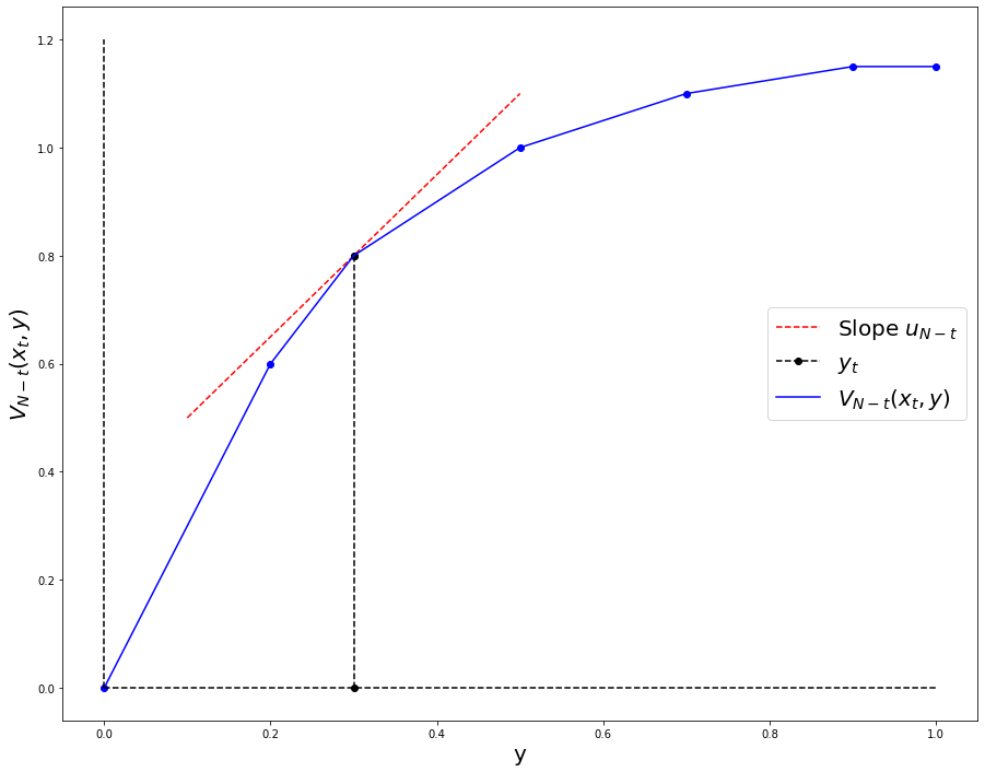
(a) Case (i): $I=1$

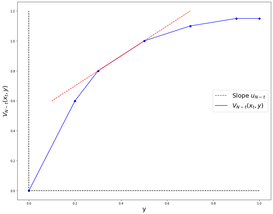
(b) Case (ii): $I=0$

Figure 1: Demonstration of Cases of Algorithm CVaR for $t>0.$

As a demonstration of Algorithm CVaR, Figure 1 shows the two main cases which were considered. Figure (1(a)) is an example of a case where there is a unique tail risk level being identified in step 2.3, and Figure (1(b)) corresponds to the other case where there is an interval with the desired slope value.

The variable $I=1$ indicates that the tail risk level $y_{t}$ is either given or identified at step 2.3 as the unique point $y^{*}$ such that $u_{N-t-1}\in\partial_{y}V_{N-t-1}(x_{t+1},y^{*}).$ The variable $I=0$ indicates that there is a nonempty open interval on which $u_{N-t-1}=d_{y}V_{N-t-1}(x_{t+1},y).$ If $N<\infty,$ then $y\mapsto V_{N-t-1}(x_{t+1},y)$ is a piecewise linear function and therefore the existence of the unique described point $y^{*}$ implies that $d^{-}_{y}V_{N-t-1}(x_{t+1},y^{*})>d^{-}_{y}V_{N-t-1}(x_{t+1},y^{*}).$ If $N<\infty$ then the algorithm stops after N iterations and returns a finite sentence of actions $a_{0},a_{1},\ldots,a_{N-1}$ implementing an optimal policy at the steps $t=0,1,\ldots,N-1.$ If $N=\infty,$ then the algorithm returns an infinite sequence of actions $a_{0},a_{1},\ldots$ implementing an optimal policy at the steps $t=0,1,\ldots,$ and the algorithm can be stopped under a finite number of iterations because the impact of additional steps will be negligibly small due to the discount factor $\beta\in[0,1),$ and estimations of stopping times are standard.

The algorithm is initialized with the value functions $V_{N}(\cdot,\cdot),$ $Q_{N}(\cdot,\cdot,\cdot),$ and consequently with the optimal action sets $A^{*}_{N}(\cdot,\cdot)$ defined by minimax equations (4.2), (4.3). If $N<\infty,$ then the functions $V_{N}(x,\cdot)$ and $Q_{N}(x,\cdot,a)$ are piecewise linear; see Subroutine 1 in Appendix B regarding constructing these functions when $N<\infty.$ As follows from (5.1) and (5.2), at steps 1 and 2.4 it is possible to choose $a_{t}\in A^{*}_{N-t}(x_{t},y_{t})$ such that $u_{N-t}=d^{-}_{y}V_{N-t}(x_{t},y_{t})$ or $u_{N-t}=d^{+}_{y}V_{N-t}(x_{t},y_{t}),$ $t=0,1,\ldots.$ This version of the algorithm does not utilize the $Q$-functions explicitly.

Tail risk levels $y_{t}$ assigned by the Nature are not available to the Decision Maker when $t>0.$ However, by using formula (5.4), which is based on the analysis of optimal policies by the Nature, at step 2.3 the algorithm detects either the tail risk level $y_{t}=y^{*}$ or an interval, in which $y_{t}$ is located, and each internal point of this interval defines the set of optimal actions for the DM, which are also optimal if the Nature selects another tail risk level from this interval. The main result of this paper is summarized in the following theorem, whose proof is provided in Section 8.

Theorem 5.1.

For an MDP with a finite number of states and actions, Algorithm CVaR implements an optimal policy. In particular, for all optimal responses from the Nature, $a_{t}\in A^{*}_{N-t}(x_{t},y_{t})$ if $0\leq t<N,$ and there is an optimal nonrandomized policy $\phi$ for the DM such that $a_{t}=\phi_{t}(x_{0},\alpha,a_{0},x_{1},a_{1},\ldots,x_{t}),$ and the policy $\phi$ minimizes $v^{1}_{N}(x_{0},\pi)+\alpha CVaR_{\alpha}(Z_{N};x_{0},\pi)$ in $\pi\in\Pi.$ In particular, if $c_{1}\equiv 0,$ then $\phi$ is the optimal policy minimizing $CVaR_{\alpha}(Z_{N};x_{0},\pi)$ for the initial state $x_{0}\in\mathbb{X}$ and for the tail risk level $\alpha\in(0,1].$

6 Properties of the Mass Transfer Problems Solved by the Nature

This section studies the problem the Nature solves at each horizon $N=1,2,\ldots$ or $N=\infty.$ The section studies problem (6.1) motivated by the maximization operation in equation (4.2). The results of this section are self-contained. Continuity, monotonicity, and concavity in $y\in[0,1]$ of the function $V(x,y)$ in formula (6.1) are assumed because, as shown in the next section, these assumptions are satisfied by the corresponding functions in (7.1). The main result of this section is Theorem 6.1, whose proof is provided in appendix B. This theorem is the key fact on which formula (5.4) in Algorithm CVaR is based.

A function $f:[a,b]\mapsto\mathbb{R},$ where $a,b\in\mathbb{R},$ is called piecewise linear, if there is a finite sequence of increasing numbers $(u_{i})_{i=0}^{n}$ with $u_{0}=a$ and $u_{n}=b$ such that the function $f$ is linear on each interval $[u_{i-1},u_{i}],$ $i=1,\ldots,n.$

Let $V:\mathbb{X}\times[0,1]\mapsto\mathbb{R}^{+}$ be a real-valued function such that for each fixed $x\in\mathbb{X}=\{1,2,\ldots,M\}$ the function is non-decreasing, continuous, and concave in $y.$ For a probability distribution $p$ on $\mathbb{X},$ that is, $p(x)\geq 0$ for all $x\in\mathbb{X}$ and $\sum_{x\in\mathbb{X}}p(x)=1$, let

$$F(y):=\max_{b\in B(y)}\sum_{x\in\mathbb{X}}V(x,yb(x))p(x),\qquad\qquad y\in[0,1],$$ (6.1)

where $B(y):=\{b\in\mathbb{R}^{M}:\ \sum_{x\in\mathbb{X}}p(x)b(x)=1,\ 0\leq yb(x)\leq 1,\ x\in\mathbb{X}\}$.

A function $\tilde{b}:[0,1]\times\mathbb{X}\to\mathbb{R}^{M}$ is called feasible for problem (6.1) if for each $x\in\mathbb{X}$ the function $y\mapsto\tilde{b}(y,x)$ is Borel-measurable on $[0,1],$ and $\tilde{b}(y,\cdot)\in B(y)$ for all $y\in[0,1].$ For example, $\tilde{b}(y,x)\equiv 1$ is a feasible function, and, if $y=0,$ then $\tilde{b}(0,x)\equiv 1$ is an optimal solutions at $y=0$ to the problem defined in (6.1). A feasible function $\tilde{b}(\cdot,\cdot)$ for problem (6.1) is called a solution to problem (6.1) if $F(y)=\sum_{x\in\mathbb{X}}V(x,y\tilde{b}(y,x))p(x)$ for all $y\in[0,1].$

For each $y\in[0,1]$ we also consider the set $B^{*}(y)=\{b\in B(y):F(y)=\sum_{x\in\mathbb{X}}V(x,yb(y))p(x)\}$ of solutions at $y.$ In other words, a feasible function $\tilde{b}:[0,1]\times\mathbb{X}\to\mathbb{R}^{M}$ is a solution if and only if $\tilde{b}(y,\cdot)\in B^{*}(y)\}$ for all $y\in[0,1].$

The following theorem describes key properties of the value functions justifying Algorithm CVaR in section 5.

Theorem 6.1.

The following statements hold for problem (6.1):

(i) there exists a solution;

(ii) the function $F$ is non-decreasing, continuous, and concave;

(iii) if $\tilde{b}(\cdot,\cdot)$ is a solution to problem (6.1), then the following relations hold for all $y\in[0,1]:$

$$\max\{d^{+}_{y}V(x,y\tilde{b}(y,x)):\,p(x)>0,\,x\in\mathbb{X}\} \leq \min\{d^{-}_{y}V(x,y\tilde{b}(y,x)):\,p(x)>0,\,x\in\mathbb{X}\}$$ (6.2)

$$F^{\prime}_{+}(y) = \max\{d^{+}_{y}V(x,y\tilde{b}(y,x)):p(x)>0,x\in\mathbb{X}\},$$ (6.3)

$$F^{\prime}_{-}(y) = \min\{d^{-}_{y}V(x,y\tilde{b}(y,x)):p(x)>0,x\in\mathbb{X}\};$$ (6.4)

(iv) if the function $V(x,y)$ is piecewise linear in $y$ for each $x\in\mathbb{X},$ then the function $F(y)$ is also piecewise linear.

Proof.

See appendix B. ∎

Problem (6.1) can be simplified to a problem, which has a natural interpretation. First, without loss of generality we can assume that $V(x,0)=0$ for all $x\in\mathbb{X},$ and therefore $V(x,y)\geq 0$ for all $x\in\mathbb{X}$ and $y\in[0,1].$ Indeed, we can always consider the objective function $\hat{V}(x,y):=V(x,y)-V(x,0).$ Then all the objective and value functions will be shifted by the constant $\sum_{x\in\mathbb{X}}V(x,0)p(x),$ and the solution sets won’t change. Second, we can assume that $p(x)>0$ for all $x\in\mathbb{X}$ because the points $x$ with $p(x)=0$ can be excluded from $\mathbb{X}.$

Third, let us consider the functions $\tilde{z}(y,x):=y\tilde{b}(y,x)p(x),$ where $y\in[0,1],$ and vectors $z(x):=yb(x)p(x),$ where $b\in\mathbb{R}^{M},$ $x\in\mathbb{X}.$ For $x\in\mathbb{X}$ and $z\in[0,p(x)],$ let us define $v(x,z):=V(x,z/p(x))p(x).$

Then problem (6.1) becomes

$$F(y):=\max_{z\in Z(y)}\sum_{x\in\mathbb{X}}v\left(x,z(x)\right),\qquad\qquad y\in[0,1],$$ (6.5)

where $Z(y):=\{z\in\mathbb{R}^{M}:\ \sum_{x\in\mathbb{X}}z(x)=y,\ 0\leq z(x)\leq p(x),\ x\in\mathbb{X}\}.$

Similarly to problem (6.1), we can consider feasible functions and solutions $\tilde{z},$ and solution sets $Z^{*}:=\{z\in Z(y):F(y)=\sum_{x\in\mathbb{X}}v(x,z(y))p(x)\}$ for problem (6.5). Then $\tilde{b}(\cdot,\cdot)$ is a solution (or feasible function) for problem (6.1) if and only if $\tilde{z}(y,x)=y\tilde{b}(y,x)p(x),$ where $y\in[0,1],$ $x\in\mathbb{X},$ is a solution (a feasible function, respectively) for problem (6.5).

Thus, in order to prove Theorem 6.1, it is sufficient to prove its version for problem (6.5) which claims properties (i)–(iv) with the following differences: a solution $\tilde{z}(\cdot,\cdot)$ to problem (6.5) should be considered in statement (iii) instead of a solution $\tilde{b}(\cdot,\cdot)$ to problem (6.1), formulae (6.2)–(6.4) become

$$\max\{d^{+}_{y}v(x,\tilde{z}(y,x)):\,x\in\mathbb{X}\} \leq \min\{d^{-}_{y}v(x,\tilde{z}(y,x)):\,x\in\mathbb{X}\}$$ (6.6)

$$F^{\prime}_{+}(y) = \max\{d^{+}_{y}v(x,\tilde{z}(y,x)):\,x\in\mathbb{X}\},$$ (6.7)

$$F^{\prime}_{-}(y) = \min\{d^{-}_{y}v(x,\tilde{z}(y,x)):\,x\in\mathbb{X}\},$$ (6.8)

and the function $v(x,y)$ should be considered in statement (iv) instead of the function $V(x,y).$

Problem (6.5) describes the following optimal mass transfer problem. For $x=1,\ldots,M,$ let us consider $M$ intervals $W(x):=\{x\}\times[0,p(x)],$ $x\in\mathbb{X},$ in $\mathbb{R}^{2},$ which we call sources. These sources can be interpreted as cylindrical vessels of the same diameter filled with a liquid up to the height $p(x).$ Let $W:=\cup_{x\in\mathbb{X}}W(x).$ There is an additional interval $[0,1],$ which we call the destination. This interval can be interpreted as an empty vertical cylindrical vessel with the same diameter and with a height 1. The total value of the liquid at source $x$ from level 0 up to the level $z\in[0,1]$ is $v(x,z),$ where $v(x,\cdot)$ is a non-decreasing concave function with $v(x,0)=0,$ $x\in\mathbb{X}.$ The goal is to fill up the destination by the liquid from sources to maximize for each $y\in[0,1]$ the total value of the liquid in the destination from the level 0 up to the level $y$. Any amount of the liquid can be taken from any part of each source.

We recall, that for a concave function $f:[a,b]\to\mathbb{R},$ where $-\infty<a<b<+\infty,$ and for $y\in[a,b]$

$$f(y)=f(a)+\int_{a}^{y}f^{\prime}_{+}(z)dz=f(a)+\int_{a}^{y}f^{\prime}_{-}(z)dz,$$

$f^{\prime}_{+}(y)\leq f^{\prime}_{-}(y),$ and the set $\{y\in[a,b]:f^{\prime}_{+}(y)<f^{\prime}_{-}(y)\}$ is denumerable. Thus, both functions $d^{+}_{y}(x,y)$ and $d^{-}_{y}(x,y),$ where $y\in[0,p(x)],$ describe the nonlinear unit price of the liquid at the source $x\in\mathbb{X}$ depending on the height $y.$ Also, since the function $v(x,\cdot)$ is non-decreasing and convex, the most valuable part of the liquid of the volume $y\in[0,p(x)]$ at the source $x\in\mathbb{X}$ is the interval $[0,y],$ whose value is $v(x,y).$ Thus, if the amounts $z(y,x)$ of liquid should be taken by an optimal policy for the level $y$ from sources $x\in\mathbb{X},$ then the decision to take all the liquid from the interval $[0,z(y,x)]$ from each source $x\in\mathbb{X}$ is optimal.

7 Properties of Value Functions and Sets of Optimal Actions.

This section describes the properties of value functions $Q_{N}(x,y,a)$ and $V_{N}(x,y)$ for RMDP3 defined in equations (4.2) and (4.3), where $N=1,2,\ldots$ or $N=\infty.$ It also describes the properties of the sets of optimal actions for the DM.

Lemma 7.1.

For $N=0,1,\ldots,$ and for $N=\infty,$ the functions $Q_{N}(x,y,a)$ and $V_{N}(x,y)$ defined in (4.2) and (4.3) are continuous, concave, and monotonically non-decreasing in $y\in[0,1]$ for all $x\in\mathbb{X}$ and $a\in A(x).$ Furthermore, if $N<\infty,$ then these functions are piecewise linear.

Proof.

For $N=0,1,\ldots$ we prove this lemma by induction. For $N=0$, the function $V_{0}(x,y)=v_{1}(x)+yv_{0}(x)$ is clearly continuous, linear, and non-decreasing in $y$ since we assume $v_{0}(x)\geq 0$ for all $x\in\mathbb{X}$.

Assume now that the lemma holds for some $N=0,1,\ldots.$ Let us rewrite (4.2) as

$$Q_{N+1}(x,y,a)=\max_{b\in B(x,y,a)}\sum_{x^{\prime}\in\mathbb{X}}(c_{1}(x,a,x^{\prime})+yb_{x^{\prime}}c(x,a,x^{\prime})+\beta V_{N}(x^{\prime},yb_{x^{\prime}}))p(x^{\prime}|x,a),$$ (7.1)

and for each $x\in\mathbb{X}$ and $a\in A(x)$ apply Theorem 6.1(ii,iv) to probabilities $p(x^{\prime}):=p(x^{\prime}|x,a)$ and to the functions

$$V(x^{\prime},y^{\prime}):=c_{1}(x,a,x^{\prime})+y^{\prime}c(x,a,x^{\prime})+\beta V_{N}(x^{\prime},y^{\prime}),\quad x^{\prime}\in\mathbb{X},y^{\prime}\in[0,1].$$ (7.2)

The function $F(y)$ defined in (6.1) for the function $V$ is equal to the function $Q_{N+1}(x,y,a)$ defined in (4.2) and rewritten in (7.1). In view of Theorem 6.1, the function $Q_{N+1}(x,y,a)$ is continuous, concave, piecewise linear, and non-decreasing in $y.$ Formula (4.3) implies that $V_{N+1}(x,y)$ is a minimum of a finite number of such functions. Therefore, the function $V_{N+1}(x,y)$ is piecewise linear, continuous, concave, and non-decreasing in $y.$ So, the lemma is proved for finite values of $N.$

In view of (A.2), non-decreasing, concave, and continuous in $y$ functions $V_{N}(x,y)$ converge uniformly to $V_{\infty}(x,y).$ Thus, $V_{\infty}(x,y)$ is nondecreasing, concave, and continuous in $y.$ Formula (7.1) for $N=\infty$ and Theorem 6.1(ii) imply that these properties also hold for $Q_{\infty}(x,y,a)$ for each $a\in A(x).$ ∎

Thus, for each $x\in\mathbb{X}$ and for each $N=0,1,\ldots$ or $N=\infty,$ the function $V_{N}(x,y)$ is concave and nonincreasing in $y$ on the interval $[0,1].$ We recall that by definition $d^{-}_{y}V_{N}(x,0)=+\infty$ and $d^{+}_{y}V_{N}(x,1)=0.$ Then for each nonnegative real number $d$ exactly one of the following to possibilities takes place: (i) either there exists a unique $y\in[0,1]$ such that $d\in\partial_{y}V_{N}(x,y)$, or (ii) there exist a unique interval $[{\bf a},{\bf b}]\subset[0,1]$ such that on this interval the function $V_{N}(x,\cdot)$ is linear with the slope $d$, and $d\notin\partial_{y}V_{N}(x,y)$ if $y\in[0,{\bf a})\cup({\bf{b}},1].$

Lemma 7.2.

Assume for $N=1,2,\ldots$ or $N=\infty$ and for some $x\in\mathbb{X}$ the value function $V_{N}(x,y)$ is linear on an interval $[{\bf a},{\bf b}],$ where $0\leq{\bf a}<{\bf b}\leq 1.$ Then the following statements hold:

1. if $a\in A^{*}_{N}(x,y)$ for some $y\in({\bf a},{\bf b}),$ then $a\in A^{*}_{N}(x,y)$ for all $y\in[{\bf a},{\bf b}];$

2. $A^{*}_{N}(x,y)=A^{*}_{N}(x,\tilde{y})$ for $y,\tilde{y}\in({\bf a},{\bf b});$

3. $d_{y}Q_{N}(x,y,a)=d_{y}V_{N}(x,y)$ for $y\in({\bf a},{\bf b})$ and $a\in A^{*}_{N}(x,y).$

Proof.

According to Lemma 7.1 the functions $V_{N}(x,y)$ and $Q_{N}(x,y,a),$ $a\in A(x),$ are concave in $y\in[0,1],$ and $V_{N}(x,y)\leq Q_{N}(x,y,a)$ for all $y\in[0,1].$ Consider statement (i) and let $a\in A^{*}_{N}(x,\tilde{y})$ for some $\tilde{y}\in({\bf a},{\bf b}).$ This means that $V_{N}(x,\tilde{y})=Q_{N}(x,\tilde{y},a).$ Since $V_{N}$ and $Q_{N}$ are concave functions, and $Q_{N}$ dominates $V_{N},$ we have that $V_{N}(x,y)=Q_{N}(x,y,a)$ for all $y\in[{\bf a},{\bf b}].$ Statements (ii) and (iii) follow from (i). ∎

8 Proof of Theorem 5.1.

This section contains the proof of Theorem 5.1.

Proof of Theorem 5.1.

For the given time horizon $N=1,2,\ldots$ or $N=1$ and for a given sequence $x_{0},x_{1},\ldots,$ the algorithm sequentially generates a finite or infinite sequence of optimal actions. Let $x_{0},x_{1},$ $x_{2},\ldots$ be the states of the system and $y_{0}=\alpha,y_{1},y_{2},\ldots$ be the tail risk levels, and the values $y_{t}$ are not observed by the DM when $t\geq 1.$ In addition to the parameters of the model, the algorithm also uses the value functions $V_{N}(\cdot,\cdot),V_{N-1}(\cdot,\cdot),\ldots,V_{N-1}(\cdot,\cdot)$, if $N<\infty,$ and it uses the value function $V_{\infty}(\cdot,\cdot)$ if $N=\infty.$

The parameter $I$ takes two values: 1 and 0. $I=1$ means that at the current time epoch $t$ the tail risk level $y_{t}$ is known, and $I=0$ indicates that it is not known. If $t=0,$ then $y_{t}=\alpha,$ and this is the case $I=1.$ If $t>1,$ then an optimal action $a_{t}\in A^{*}_{N-t}(x_{t},y_{t})$ at epoch $t$ is chosen by the algorithm in step 2.4 after the algorithm either detects $y_{t}$ or detects that $y_{t}$ belongs to a linear interval with the slope defined in formula (5.4).

Let an optimal action $a_{t}\in A^{*}_{N-t}(x_{t},y_{t})$ be selected at an epoch $t=0,1,\ldots$ by step 1 or 2.4 of the algorithm. Then

$$V_{N-t}(x_{t},y_{t})=Q_{N-t}(x_{t},y_{t},a_{t})=\max_{b\in B(x_{t},y_{t},a_{t})}\sum_{x^{\prime}\in\mathbb{X}}V(x^{\prime},y_{t}b_{x^{\prime}})p(x^{\prime}|x_{t},a_{t}),$$

where the function $V$ is defined in (7.2) with $N:=N-t-1.$ Formula (6.3) implies

$$\begin{array}[]{ll}d^{+}_{y}Q_{N-t}(x_{t},a_{t},y_{t})&=\max\{c(x_{t},a_{t},x^{\prime})+\beta d^{+}_{y}V_{N-t-1}(x^{\prime},y_{t}b_{x^{\prime}}):\,x^{\prime}\in\mathbb{X},\ p(x^{\prime}|x_{t},a_{t},x^{\prime})>0\}\\ &\geq c(x_{t},a_{t},x_{t})+\beta d^{+}_{y}V_{N-t-1}(x_{t+1},y_{t+1}),\end{array}$$

where the last inequality holds because $x_{t+1}\in\mathbb{X},$ and $y_{t+1}=y_{t}b_{x_{t+1}}$ for every $b\in B^{*}(x_{t},y_{t},a_{t}).$ Thus,

$$d^{+}_{y}V_{N-t-1}(x_{t+1},y_{t+1})\leq\frac{d^{+}_{y}Q_{N-t}(x_{t},a_{t},y_{t})-c(x_{t},a_{t},x_{t+1})}{\beta}.$$ (8.1)

Similarly to (8.1), formula (6.4) implies

$$\frac{d^{-}_{y}Q_{N-t}(x_{t},a_{t},y_{t})-c(x_{t},a_{t},x_{t+1})}{\beta}\leq d^{-}_{y}V_{N-t-1}(x_{t+1},y_{t+1}).$$ (8.2)

In addition, $d^{+}_{y}Q_{N-t}(x_{t},a_{t},y_{t})\leq d^{-}_{y}Q_{N-t}(x_{t},a_{t},y_{t}).$ Therefore, in view of inequalities (8.1) and (8.2),

$$u_{N-t-1}:=\frac{u_{N-t}-c(x_{t},a_{t},x_{t+1})}{\beta}\in\partial_{y}V_{N-t-1}(x_{t+1},y_{t+1})$$ (8.3)

for $u_{N-t}:=d^{-}_{y}Q_{N-t}(x_{t},a_{t},y_{t})$ and for $u_{N-t}:=d^{+}_{y}Q_{N-t}(x_{t},a_{t},y_{t}).$ If there is a unique point $y^{*}$ such that $u_{N-t-1}\in\partial_{y}V_{N-t-1}(x_{t+1},y^{*}),$ then $y_{t+1}=y^{*}$ is the tail risk level at the state $x_{t+1}$ and epoch $(t+1).$

If there are multiple points $y^{*}$ such that $u_{N-t-1}\in\partial_{y}V_{N-t-1}(x_{t+1},y^{*}),$ that is, the case $I=0$ takes place, then concavity of $V_{N-t-1}(x_{t+1},\cdot)$ implies that there is a maximal interval $[{\bf a},{\bf b}]\subset[0,1]$ such that the function $V_{N-t-1}(x_{t+1},y)$ is linear in $\in[{\bf a},{\bf b}],$ and its slope is $u_{N-t-1}.$ According to Lemma 7.2, for all $y\in({\bf a},{\bf b})$ the sets $A^{*}_{N-t-1}(x_{t+1},y)$ coincide, and $d_{y}Q_{N-t-1}(x_{t+1},y,a)=d_{y}V_{N}(x_{t+1},y)$ for $a\in A^{*}_{N-t-1}(x_{t+1},y).$ Therefore, step 2.1 can be skipped, and future calculations do not depend on the particular value $y_{t+1}\in({\bf a},{\bf b}).$ So, $a_{t}\in A^{*}_{N-t}(x_{t},y_{t})$ in spite of the fact that the DM does not know the states $y_{t}$ when $t>0.$ The algorithm either calculates values $y_{t}$ or can calculate intervals to which values $y_{t}$ belong, and optimal action sets coincides for tail risk levels on these intervals. ∎

Appendix A Results on Robust MDPs Used in this Paper

This appendix describes results on RMDPs and relevant facts used in this paper. In general, for robust optimization problems, some parameters of the model are unknown, and the goal is to select the best solutions for the worst possible values of unknown parameters. Starting from [14] and [20] there are numerous studies of RMDPs. Here we are interested in models when in addition to the state and action, there is the third parameter on which one-step costs and transition probabilities depend, and the Nature can select this parameter from a set of available parameters. The DM chooses actions by knowing the past and current states and the past actions chosen by the DM and by the Nature. The Nature chooses actions by knowing the same information and, in addition, by knowing the current action chosen by the DM. Such robust optimization models were also studied under the names of games with perfect information (see e.g., [9, 1, 15]) and minimax control [10].

For the purposes of this paper, it is sufficient to consider an RMDP with a state space being a compact subset of a Euclidean space, a finite action space for the DM, and action sets of the Nature being compact subsets of a Euclidean space. In addition, one-step cost functions are continuous. Transition probabilities are weakly continuous. We consider in this appendix a slightly more general model. This section is mostly based on the description of the two-player game, in which Player I is the DM, and Player II is the Nature.

An RMDP is defined by a tuple $({\bf X},\mathbb{A},\mathbb{B},A(\cdot),B(\cdot,\cdot),c,p).$ Here ${\bf X}$ is the state space, and there are two players and two decision sets $\mathbb{A}$ and $\mathbb{B},$ where $\mathbb{A}$ is the set of actions for Player I, and $\mathbb{B}$ is the set of actions for Player II. We assume that ${\bf X},$ $\mathbb{A}$, and $\mathbb{B}$ are nonempty Borel subsets of Polish (complete, separable, metric) spaces. The sets $\mathbb{A}$ and $A(x)\subset\mathbb{A},$ where $x\in{\bf X},$ are nonempty and finite, and $A(x)$ is the set of actions available to Player I at states $x.$ For each pair $(x,a)$ such that $x\in{\bf X}$ and $a\in A(x),$ a set of feasible actions $B(x,a)$ of Player II is defined. We assume that the sets $B(x,a)$ are nonempty and compact subsets of $\mathbb{B}$ for all $x\in{\bf X}$ and for all $a\in A(x).$ We also assume that the set ${\rm Gr}\ A:=\{(x,a):\,x\in{\bf X},a\in A(x)\}$ is a Borel subset of ${\bf X}\times\mathbb{A},$ and the set ${\rm Gr}\ B:=\{(x,a,b):\,x\in{\bf X},a\in A(x),b\in B(x,a)\}$ is a Borel subset of ${\bf X}\times\mathbb{A}\times\mathbb{B}.$ The one-step cost function is $c:{\bf X}\times\mathbb{A}\times\mathbb{B}\mapsto\mathbb{R}$ is assumed to be bounded and continuous. The transition probability $p$ from ${\bf X}\times\mathbb{A}\times\mathbb{B}$ to ${\bf X}$ is weakly continuous in $(x,a,b)\in{\bf X}\times\mathbb{A}\times\mathbb{B}.$ We also assume that the set-valued mappings $A:{\bf X}\mapsto 2^{\mathbb{A}}$ and $B:{\bf X}\times\mathbb{A}\mapsto 2^{\mathbb{B}}$ are continuous.

At each time step, Player II knows the decision of Player I at the time Player II makes a decision. Let $H_{t}:=({\bf X}\times\mathbb{A}\times\mathbb{B})^{t}\times{\bf X}$ be the sets of histories that can be observed by Player I at time steps $t=0,1,\ldots.$ The sets of histories that can be observed by Player II at steps $t=0,1,\ldots$ are $H_{t}\times\mathbb{A}.$ A policy $\pi^{\mathbb{A}}$ of Player I is a sequence $(\pi^{\mathbb{A}}_{t})_{t=0.1,\ldots}$ of regular transition probabilities from $H_{t}$ to $\mathbb{A}$ such that $\pi^{\mathbb{A}}_{t}(A(x_{t})|x_{0},a_{0},b_{0},\ldots,x_{t-1},a_{t-1},b_{t-1},x_{t})=1.$ A policy $\pi^{\mathbb{B}}$ of Player I is a sequence $(\pi^{\mathbb{B}}_{t})_{t=0.1,\ldots}$ of regular transition probabilities from $H_{t}\times\mathbb{A}$ to $\mathbb{B}$ such that $\pi^{\mathbb{B}}_{t}(B(x_{t},a_{t})|x_{0},a_{0},b_{0},\ldots,x_{t-1},a_{t-1},b_{t-1},x_{t},a_{t})=1.$ Let $\Pi^{\mathbb{A}}$ and $\Pi^{\mathbb{B}}$ be the sets of policies for Player I and for Player II respectively. Similarly to MDPs, an initial state $x\in{\bf X}$ and a pair of policies $(\pi^{\mathbb{A}},\pi^{\mathbb{B}})\in\Pi^{\mathbb{A}}\times\Pi^{\mathbb{B}}$ define the probability $P_{x}^{\pi^{\mathbb{A}},\pi^{\mathbb{B}}}$ on the space of trajectories $H:=({\bf X}\times\mathbb{A}\times\mathbb{B})^{\infty}.$ An expectation with respect to this probability is denoted by $\mathbb{E}_{x}^{\pi^{\mathbb{A}},\pi^{\mathbb{B}}}.$

It is also possible to consider nonrandomized, Markov, and deterministic policies. A policy $\pi^{\mathbb{A}}$ for Player I is called nonrandomized if for each $t=0,1,\ldots$ there exists a mapping $\phi^{\mathbb{A}}_{t}:H_{t}\to\mathbb{A}$ such that $\pi^{\mathbb{A}}_{t}(\phi^{\mathbb{A}}_{t}(h_{t})|h_{t})=1$ for all $h_{t}=x_{0},a_{0},b_{0},\ldots,x_{t-1},a_{t-1},b_{t-1},x_{t}\in H_{t}.$ Such a policy is also denoted by $\phi^{\mathbb{A}}.$ A Markov policy $\phi^{\mathbb{A}}$ for Player I is a sequence of measurable functions $\phi_{t}^{\mathbb{A}}:{\bf X}\to\mathbb{A},$ $t=0,1,\ldots,$ such that $\phi_{t}^{\mathbb{A}}(z)\in A(z)$ for all $z\in{\bf X}.$ A deterministic policy for Player I is a Markov policy $\phi^{\mathbb{A}}$ such that $\phi^{\mathbb{A}}_{t}(z)=\phi^{\mathbb{A}}_{s}(z)$ for all $t,s=0,1,\ldots$ and all $z\in\bf{X}.$

A policy $\pi^{\mathbb{B}}$ for Player II is called nonrandomized, if for each $t=0,1,\ldots$ there exists a mapping $\phi^{\mathbb{B}}_{t}:H_{t}\times\mathbb{A}\to\mathbb{B}$ such that $\pi^{\mathbb{B}}_{t}(\phi^{\mathbb{B}}_{t}(h_{t},a_{t})|h_{t},a_{t})=1$ for all $h_{t}=x_{0},a_{0},b_{0},\ldots,x_{t-1},a_{t-1},b_{t-1},x_{t},a_{t}\in H_{t}\times\mathbb{A}.$ Such a policy is also denoted by $\phi^{\mathbb{B}}.$ A Markov policy $\phi^{\mathbb{B}}$ for Player II is a sequence of measurable functions $\phi_{t}^{\mathbb{A}}:{\bf X}\times\mathbb{A}\to\mathbb{B},$ $t=0,1,\ldots,$ such that $\phi_{t}^{\mathbb{B}}(z,a)\in B(z,a)$ for all $(z,a)\in{\bf X}\times\mathbb{A}.$ A deterministic policy for Player II is a Markov policy $\phi^{\mathbb{B}}$ such that $\phi^{\mathbb{B}}_{t}(z,a)=\phi^{\mathbb{B}}_{s}(z,a)$ for all $t,s=0,1,\ldots$ and all $(z,a)\in\bf{X}\times\mathbb{A}.$

If an initial state is $x\in{\bf X}$ and Players I and II play policies $\pi^{\mathbb{A}}$ and $\pi^{\mathbb{B}}$ respectively, then the expected total finite-horizon payoff of Player I to Player II is

$$v_{N}(x,\pi^{\mathbb{A}},\pi^{\mathbb{B}}):=\mathbb{E}_{x}^{\pi^{\mathbb{A}},\pi^{\mathbb{B}}}[\sum_{t=0}^{N-1}\beta^{t}c(x,a_{t},b_{t})+v_{0}(x_{N})],\quad N=1,2,\ldots,\ \beta\in[0,1],$$

where $v_{0}:{\bf X}\mapsto\mathbb{R}$ is a bounded continuous function, and for the infinite horizon

$$v_{\infty}(x,\pi^{\mathbb{A}},\pi^{\mathbb{B}}):=\mathbb{E}_{x}^{\pi^{\mathbb{A}},\pi^{\mathbb{B}}}\left[\sum_{t=0}^{\infty}\beta^{t}c(x,a_{t},b_{t})\right],\quad\beta\in[0,1).$$

For $\beta\in[0,1]$ and $N=0,1,\ldots,$ let us define sequentially

$$v_{N+1}(x)=\min_{a\in\mathbb{A}(x)}\max_{b\in B(x,a)}\{c(x,a,b)+\beta\int_{\bf X}v_{N}(x^{\prime})p(dx^{\prime}|x,a,b)\},\quad x\in{\bf X}.$$ (A.1)

For $\beta\in[0,1),$ Banach’s fixed point theorem implies that for $N=\infty$ equation (A.1) has a unique bounded solution $v_{\infty}(x),$ and $v_{N}(x)\to v_{\infty}(x)$ as $N\to\infty.$ In particular

$$\sup_{x\in\bf{X}}|v_{N}(x)-v_{\infty}(x)|\leq C\beta^{N}/(1-\beta)\to 0\ {\rm as}\ N\to\infty,$$ (A.2)

where $C=\sup\{c(x,a,b):\,(x,a,b)\in{\rm Gr}\ B\}.$ In view of the Berge maximum theorem, the functions $v_{N}(x),$ $N=1,2,\ldots,$ are continuous. Therefore, their uniform pointwise limit $v_{\infty}(x)$ is continuous too. Thus, the internal maximum in (A.1) is achieved.

For $N=1,2,\ldots$ or $N=\infty$ let us consider the following nonempty sets of actions for Players I and II respectively

$$A^{*}_{N}(x):=\bigl{\{}a\in A(x):\,v_{N}(x)=\max_{b\in B(x,a)}\{c(x,a,b)+\beta\int_{\bf X}v_{N-1}(x^{\prime})p(dx^{\prime}|x,a,b)\}\bigr{\}},\ x\in{\bf X},$$ (A.3)

and

$$B^{*}_{N}(x,a) :=\bigl{\{}b^{*}\in B(x,a):\,c(x,a,b^{*})+\beta\int_{\bf X}v_{N-1}(x^{\prime})p(dx^{\prime}|x,a,b^{*})$$ (A.4)

$$=\max_{b\in B(x,a)}\{c(x,a,b)+\beta\int_{\bf X}v_{N-1}(x^{\prime})p(dx^{\prime}|x,a,b)\}\bigr{\}},\ x\in{\bf X}.$$

The sets $A_{N}^{*}(x)$ are finite and, as follows from the Berge maximum theorem, the sets $B_{N}^{*}(x,a)$ are compact.

For an $N$-horizon problem with $N=1,2,\dots$ or $N=\infty,$ a pair of policies $(\pi^{\mathbb{A}}_{*},\pi^{\mathbb{B}}_{*})\in\Pi^{\mathbb{A}}\times\Pi^{\mathbb{B}}$ is called equilibrium at the initial state $x\in{\bf X},$ if for all policies $\pi^{\mathbb{A}}\in\Pi^{\mathbb{A}}$ and $\pi^{\mathbb{B}}\in\Pi^{\mathbb{B}}$

$$v_{N}(x,\pi^{\mathbb{A}}_{*},\pi^{\mathbb{B}})\leq v_{N}(x,\pi^{\mathbb{A}}_{*},\pi^{\mathbb{B}}_{*})\leq v_{N}(x,\pi^{\mathbb{A}},\pi^{\mathbb{B}}_{*}).$$

A pair $(\pi^{\mathbb{A}}_{*},\pi^{\mathbb{B}}_{*})\in\Pi^{\mathbb{A}}\times\Pi^{\mathbb{B}}$ is equilibrium if it is equilibrium at each $x\in{\bf X}.$ If a pair $(\pi^{\mathbb{A}}_{*},\pi^{\mathbb{B}}_{*})\in\Pi^{\mathbb{A}}\times\Pi^{\mathbb{B}}$ is an equilibrium, then $\pi^{\mathbb{A}}_{*}$ is called an optimal policy of Player I, and $\pi^{\mathbb{B}}_{*}$ is called an optimal policy of Player II.

The key facts are that for a finite horizon $N$ there exist pairs of Markov equilibrium policies, and for $N=\infty$ these policies can be chosen to be deterministic. In addition, these policies have certain structural properties, and their optimality can be defined in a stronger sense called persistent optimality.

For a Markov policy $\phi=(\phi_{0},\phi_{1},\ldots)$ and for $t=0,1,\ldots,$ let us denote by $\phi_{[t]}$ the Markov policy $\phi_{[t]}:=(\phi_{t},\phi_{t+1},\ldots).$ Of course, $\phi_{[0]}=\phi.$ This notations applies to both players.

For an $N$-horizon problem with $N=1,2,\dots$ or $N=\infty,$ a pair of Markov policies $(\phi^{\mathbb{A}},\phi^{\mathbb{B}})\in\Pi^{\mathbb{A}}\times\Pi^{\mathbb{B}}$ is called persistently equilibrium if for all initial states $x\in{\bf X},$ for all policies $\pi^{\mathbb{A}}\in\Pi^{\mathbb{A}}$ and $\pi^{\mathbb{B}}\in\Pi^{\mathbb{B}},$ for all nonnegative integers $t$ satisfying $0\leq t<N$

$$v_{N-t}(x,\phi^{\mathbb{A}}_{[t]},\pi^{\mathbb{B}}_{[t]})\leq v_{N-t}(x,\phi^{\mathbb{A}}_{[t]},\pi^{\mathbb{B}}_{[t]})\leq v_{N-t}(x,\pi^{\mathbb{A}}_{[t]},\pi^{\mathbb{B}}_{[t]}).$$

For an infinite-horizon problem, a pair of deterministic (that is, nonrandomized stationary) policies is persistently equilibrium if and only if it is equilibrium.

For all $N=1,2,\ldots$ and $N=\infty,$ for every policy $\pi^{\mathbb{A}}\in\Pi^{\mathbb{A}}$ there exists a policy $\pi^{\mathbb{B},N}\in\Pi^{\mathbb{B}},$ and for every policy $\pi^{\mathbb{B}}\in\Pi^{\mathbb{B}}$ there exists a policy $\pi^{\mathbb{A},N}\in\Pi^{\mathbb{A}},$ such that

$$v_{N}(x,\pi^{\mathbb{A}},\pi^{\mathbb{B},N})=\max_{{\tilde{\pi}}^{\mathbb{B}}\in\Pi^{\mathbb{B}}}v_{N}(x,\pi^{\mathbb{A}},{\tilde{\pi}}^{\mathbb{B}})\qquad{\rm and}\qquad v_{N}(x,\pi^{\mathbb{A},N},\pi^{\mathbb{B}})=\min_{{\tilde{\pi}}^{\mathbb{A}}\in\Pi^{\mathbb{A}}}v_{N}(x,{\tilde{\pi}}^{\mathbb{A}},\pi^{\mathbb{B}})$$ (A.5)

Let us prove the second equality in (A.5). Let us fix a policy $\pi^{\mathbb{B}}\in\Pi^{\mathbb{B}}.$ Then Player I should minimize the expected total discounted cost for an MDP with the state space $H:=\cup_{\{t=0,1,\ldots\}}H_{t},$ where $H_{t}=({\bf X}\times\mathbb{A}\times\mathbb{B})^{t}\times{\bf X},$ $t=0,1,\ldots,$ action space $\mathbb{A}^{\mathbb{A}}:=\mathbb{A},$ the sets of available actions $A(h_{t})=A(x_{t}),$ where $h_{t}=x_{0},a_{0},b_{0},\ldots,x_{t}\in H_{t},$ one-step costs $c(h_{t},a)=\int_{\mathbb{B}}c(x_{t},a,b)\pi_{t}^{\mathbb{B}}(db|h_{t},a),$ and transition probabilities defined by $p(h_{t},a,B,x^{\prime}|h_{t},a)=\int_{B}p(x^{\prime}|x_{t},a,b)\pi_{t}^{\mathbb{B}}(db|h_{t},a),$ where $a\in A(x_{t}),$ $B\in\mathcal{B}(\mathbb{B}),$ and $x^{\prime}\in{\bf X}.$ This is an MDP with finite action sets, bounded costs, and with the goal to minimize the expected total costs. For this MDP there exists an optimal policy; see e.g., [7, Theorem 3.1]. In particular, it is optimal for all initial states $x\in{\bf X}\subset H.$ Therefore, the second equality in (A.5) holds.

Let us prove the first equality in (A.5). Let us fix a policy $\pi^{\mathbb{A}}\in\Pi^{\mathbb{A}}.$ Then Player II should maximize the expected total discounted rewards for an MDP with the state space $H\times\mathbb{A},$ action space $\mathbb{B},$ sets of available actions $B(h_{t},a)=B(x_{t},s,b),$ where $h_{t}=x_{0},a_{0},b_{0},\ldots,x_{t}\in H_{t},$ $t=0,1,\ldots,$ one-step rewards $c(h_{t},a,b)=c(x_{t},a,b),$ and transition probabilities defined by $p(h_{t},a,b,x^{\prime},a^{\prime}|h_{t},a,b)=p(x^{\prime}|x_{t},a,b)\pi_{t+1}^{\mathbb{A}}(a^{\prime}|h_{t},a,b,x^{\prime}),$ where $a\in A(x_{t}),$ $b\in B(x_{t},a),$ $x^{\prime}\in{\bf X},$ and $a^{\prime}\in A(x^{\prime}).$ This is an MDP with compact action sets, bounded continuous one-step costs, weakly continuous transition probabilities, and the goal is to maximize the expected total discounted rewards. For this MDP there exists an optimal policy; see e.g., [8, Theorem 2]. In particular, for each $x\in{\bf X},$ the optimal policy is optimal for the initial state distribution $\mu$ on ${\bf X}\times\mathbb{A}$ defined by $\mu(x,a)=\pi_{0}^{\mathbb{A}}(a|x),$ where $a\in A(x).$ Therefore, the first equality in (A.5) holds.

For a finite horizon $N=1,2,\ldots$ there exists a pair of Markov policies $(\phi^{\mathbb{A},N},\phi^{\mathbb{A},N})$ for Players I and II respectively, which forms a persistent equilibrium. In addition, a Markov policy $\phi^{\mathbb{A},N}$ is persistently optimal for Player I if and only if

$$\phi_{t}^{\mathbb{A},N}(x)\in A^{*}_{N-t}(x)\quad{\rm for\ all}\ x\in{\bf X},\ t=0,1,\ldots,N-1,$$ (A.6)

and a Markov policy $\phi^{\mathbb{B},N}$ is persistently optimal for Player II if and only if

$$\phi_{t}^{\mathbb{B},N}(x,a)\in B^{*}_{N-t}(x,a)\quad{\rm for\ all}\ x\in{\bf X},\ a\in A(x),\ t=0,1,\ldots,N-1,$$ (A.7)

In addition, a pair of Markov policies $(\phi^{\mathbb{A},N},\phi^{\mathbb{B},N})$ for Players I and II forms a persistent equilibrium if and only if $\phi^{\mathbb{A},N}$ and $\phi^{\mathbb{B},N}$ are persistently optimal policies for Players I and II respectively. Correctness of these claims follows from the standard dynamic programming arguments including induction in $N$ starting from $N=1$ and from the arguments described in the following two paragraphs.

First, let Player I choose a Markov policy $\phi^{\mathbb{A},N}$ satisfying (A.6). Then Player II should maximize the expected total rewards for an $N$-horizon MDP defined by this policy. This MDP can be defined as an MDP with states $(x,a,n),$ where $x\in{\bf X},$ $a\in A(x),$ $n=N,N-1,\ldots,0,$ the action space $\mathbb{B},$ sets of available actions $B(x,a,n):=B(x,a)$, one-step rewards $c(x,a,n,b)=c(x,a,b),$ if $n>1$, $c(x,a,1,b,x^{\prime})=c(x,a,b)+\beta v_{0}(x^{\prime}),$ and $c(x,a,0,b)=0,$ and transition probabilities defined by $p(x^{\prime},\phi_{N-n+1}^{\mathbb{A},N}(x^{\prime}),n-1|x,a,n,b)=p(x^{\prime}|x,a,b)$ for $N=N,N-1,\ldots,1,$ and $p(x,a,0|x,a,0,b)=1.$ In other words, the MDP stops after $N$ moves or, which is equivalent, after it gets to states $(x,a,0).$ Then formula (A.7) defines the sets of Markov persistently optimal policies; see [8, Theorem 2], where a more general model is considered.

Second, let Player II chooses a Markov policy $\phi^{\mathbb{B},N}$ satisfying (A.7). Then Player I should minimize the expected total costs for an $N$-horizon MDP defined by this policy. This MDP can be defined as an MDP with states $(x,n),$ where $x\in{\bf X},$ $n=N,N-1,\ldots,0,$ the action space $\mathbb{A},$ sets of available actions $A(x,n):=A(x)$, one-step costs $c(x,n,a)=c(x,a,\phi_{N-n}^{\mathbb{B},N}),$ if $n>1$, $c(x,1,a,x^{\prime})=c(x,a,\phi_{N-n}^{\mathbb{B},N})+\beta v_{0}(x^{\prime}),$ and $c(x,0,a)=0,$ and transition probabilities defined by $p(x^{\prime},n-1|x,n,a)=p(x^{\prime}|x,a,\phi_{N-n}^{\mathbb{B},N})$ for $N=N,N-1,\ldots,1,$ and $p(x,0|x,0,a)=1.$ The MDP stops after $N$ moves or, which is equivalent, stops after it gets to states $(x,a,0).$ Then formula (A.6) defines the sets of Markov persistently optimal policies; see [7, Theorem 3.1]. These constructions also imply that

$$v_{N}(x,\phi^{\mathbb{A},N},\phi^{\mathbb{B},N})=v_{N}(x),\qquad x\in{\bf X},$$ (A.8)

for Markov equilibrium policies $(\phi^{\mathbb{A},N},\phi^{\mathbb{B},N}),$ where $N=1,2,\ldots.$

For an infinite horizon problem, that is, for $N=\infty,$ there is a pair of deterministic equilibrium policies $(\phi^{\mathbb{A},\infty},\phi^{\mathbb{B},\infty})$ for Players I and II respectively. Indeed, for $N=\infty$ let us consider the sets of optimal actions $A_{\infty}^{*}(x)$ and $B_{\infty}^{*}(x,a)$ for Players I and II, where $x\in X$ and $a\in A(x).$ A pair of deterministic policies $(\phi^{\mathbb{A},\infty},\phi^{\mathbb{B},\infty})$ for Players I and II form an equilibrium if and only if $\phi^{\mathbb{A},\infty}$ and $\phi^{\mathbb{B},\infty}$ are optimal policies for Players I and II respectively for $N=\infty.$ This is true because of the arguments provided in the following paragraph. These arguments are similar to the arguments in a finite-horizon case, but the constructions of MDPs are simpler for the infinite-horizon case.

If Player I chooses a deterministic policy $\phi^{\mathbb{A},\infty}$ satisfying (A.6) with $N=\infty,$ then Player II should maximize the expected total rewards for an infinite-horizon MDP with states $(x,a),$ where $x\in{\bf X},$ $a\in A(x),$ the action space $\mathbb{B},$ sets of available actions $B(x,a)$, one-step rewards $c(x,a,b),$ and transition probabilities defined by $p(x^{\prime},\phi^{\mathbb{A},\infty}(x^{\prime})|x,a,b)=p(x^{\prime}|x,a,b).$ Then formula (A.7) with $N=\infty$ defines the set of deterministic optimal policies for Player II; see [8, Theorem 2]. If Player II chooses a deterministic policy $\phi^{\mathbb{B},\infty}$ satisfying (A.7) with $N=\infty,$ then Player I should minimize the expected total costs for an infinite-horizon MDP with the state space ${\bf X},$ $n=N,N-1,\ldots,0,$ the action space $\mathbb{A},$ sets of available actions $A(x)$, one-step costs $c(x,a)=c(x,a,\phi^{\mathbb{B},\infty}),$ and transition probabilities defined by $p(x^{\prime}|x,a)=p(x^{\prime}|x,a,\phi^{\mathbb{B},\infty}(x,a)).$ Then formula (A.6) with $N=\infty$ defines the sets of deterministic optimal policies for Player I; see [8, Theorem 2]. These constructions also imply that formula (A.8) holds with $N=\infty$ for a pair of deterministic equilibrium policies $(\phi^{\mathbb{A},\infty},\phi^{\mathbb{B},\infty}).$

The function $x\mapsto v_{N}(x)$ is called the value function for $N=1,2,\ldots$ and for $N=\infty.$ Under the assumptions formulated in this section, the following equalities take place

$$v_{N}(x)=\min_{\pi^{\mathbb{A}}\in\Pi^{\mathbb{A}}}\max_{\pi^{\mathbb{B}}\in\Pi^{\mathbb{B}}}v_{N}(x,\pi^{\mathbb{A}},\pi^{\mathbb{B}})=\max_{\pi^{\mathbb{B}}\in\Pi^{\mathbb{B}}}\min_{\pi^{\mathbb{A}}\in\Pi^{\mathbb{A}}}v_{N}(x,\pi^{\mathbb{A}},\pi^{\mathbb{B}}),\quad x\in{\bf X}.$$ (A.9)

Correctness of (A.9) follows from the following two observations: (i) (A.9) holds with $\min$ and $\max$ replaced with $\inf$ and $sup$ respectively, and (ii) $\inf$ and $\sup$ operations mentioned in (i) can be replaced with $\min$ and $\max$ respectively. Statement (i) follows from the following two facts: (a) [15, Theorem 4], claiming equalities similar to (A.9) with $\inf$ and $\sup$ instead of $\min$ and $\max$ respectively for games with simultaneous moves, compact action sets for Player I, and possibly noncompact action sets for Player II, (b) a stochastic game with perfect information described in this section can be reduced to a stochastic game with simultaneous moves. This is true because a game with perfect information can be reduced to a turn-based game, as is explained in this paragraph, and the turn-based game can be formally presented as a game with simultaneous move, when at each step one of the players has a single action. Let us provide some details. One unit of time in the original game with perfect information corresponds to two units of time in the equivalent turn-based game. Therefore the discount factor in the new game is $\beta^{\frac{1}{2}}$ if $\beta>0$ is the discount factor for the original game. If $\beta=0$ then the original game consists just of one move. Then the new game will be defined only for two moves with the discount factor $\beta=1.$ For this reduction, let us define the state space ${\bf X}\cup{\rm Gr}\ A.$ States $x\in{\bf X}$ are controlled by Player I whose set of feasible actions are $A(x),$ the transition probability is defined by $p((x,a)|x,a)=1,$ and the one-step cost is $c(x,a)=0,$ where $a\in A(x).$ States $(x,a)\in{\rm Gr}\ A$ are controlled by Player II whose sets of feasible actions are $B(x,a)$, the transition probability is defined by $p(x^{\prime}|x,a,b),$ and the one-step cost is $\beta^{-\frac{1}{2}}c(x,a,b),$ where $b\in B(x,a),$ where $\beta>0$ is the discount factor. In order to complete this construction to make it a stochastic game with simultaneous moves, we also add a single fictitious action for Player II at states $x\in{\bf X}$ and a single fictitious action for Player I at states $(x,a)\in{\rm Gr}\ A.$ Being applied to this game, [15, Theorem 4] implies formula (A.9) with $\inf$ and $\sup$ operators. The internal $\inf$ and $\sup$ can be replaced with $\min$ and $\max$ respectively in view of formulae (A.5). The existence of an equilibrium pair implies that the external $\inf$ and $\sup$ can be also replaced with $\min$ and $\max.$

We remark that it is also possible to consider pairs of non-Markov equilibrium and persistently equilibrium policies. It is possible to show that for an $N$-horizon problem with $N=1,2,\ldots$ or $N=\infty$, a policy $\pi^{\mathbb{A}}\in\Pi^{\mathbb{A}}$ is persistently optimal for Player I if and only if $\pi^{\mathbb{A}}(A^{*}_{N-t}(x_{t})|h_{t})=1,$ for all $0\leq t<N$ and for all $h_{t}=x_{0},a_{0},b_{0},\ldots,x_{t}.$ A policy $\pi^{\mathbb{B}}\in\Pi^{\mathbb{B}}$ is persistently optimal for Player II if and only if $\pi^{\mathbb{B}}(B^{*}_{N-t}(h_{t},a_{t})|h_{t})=1,$ for all $0\leq t<N$ for all $h_{t}=x_{0},a_{0},b_{0},\ldots,x_{t},$ and for all $a_{t}\in\mathbb{A}(x_{t}),$ where $\pi^{\mathbb{B}}\in\Pi^{\mathbb{B}}.$ The proofs of these observations follow from considering MDPs with state spaces $H$ and $H\times\mathbb{A}$ above introduced to prove equalities (A.5).

The definition of persistently equilibrium pairs of policies for games with perfect information is consistent with the definition of persistently optimal policies for MDPs. An MDP can be viewed as a game with perfect information when the action space $\mathbb{B}$ for Player II is a singleton, and the parameter $b$ is omitted from notations. A Markov policy $\phi$ is persistently optimal for an $N$-horizon discounted MDP, $N=1,2,\ldots$ or $N=\infty,$ with the state space $X$ and with the expected total discounted costs $v_{N}(x)$ if $v_{N}(x,\phi_{[t]})=v_{N}(x)$ for all $x\in X$ and for all $0\leq t<N+1.$

In particular, persistently optimal policies exist for an MDP $\{X,A,A(\cdot),c,p)\},$ if the state space $X$ is a Borel subset of a Polish space, the sets of all actions $A$ and the sets of all available actions A(x), $x\in{\bf X},$ are nonempty compact subsets of a Polish space, the set-valued mapping $x\mapsto A(x)$ is upper semicontinuous, one step costs $c(x,a)$ are bounded and continuous, and transition probabilities $p(\cdot|x,a)$ are weakly continuous in $(x,a).$ This fact follows from [8, Theorem 2], where a more general MDP is considered. In addition, the optimality equations for finite and infinite-step problems are

$$v_{N+1}(x)=\min_{a\in A(x)}\{c(x,a)+\beta\int_{\bf{X}}v_{N}(x^{\prime})p(dx^{\prime}|x,a)\},\quad x\in{\bf X},\ N=0,1,\ldots\ {\rm or}\ N=\infty,$$ (A.10)

where $v_{0}$ is the given bounded lower semicontinuous function on $\bf{X}.$ Optimality equations define the sets of optimal actions

$$A_{N}(x):=\{a\in A(x):\,V_{N}(x)=c(x,a)+\beta\int_{\bf{X}}V_{N-1}(x^{\prime})p(dx^{\prime}|x,a)\},\quad x\in\bf{X}.$$

A Markov policy $\phi$ is persistently optimal for an $N$-horizon problem with $N=1,2,\ldots$ or $N=\infty,$ if and only if $\phi_{t}(x)\in A_{N-t}(x)$ for all nonnegative integers $t$ satisfying $t<N,$ where, for an integer $s\geq 1$ satisfying $s<N+1.$ A deterministic policy $\phi$ is optimal for an infinite-horizon problem if and only if $\phi(x)=A_{\infty}(x)$ for all $x\in X.$

We remark that, since this section deals with risk-neutral problems, we usually consider in it one-step costs, which do not depend on the next state. Similar to risk-neutral MDPs, one-step costs $c(x,a,b,x^{\prime})$ can be considered for games, and they can be reduced to one-step costs $c(x,a,b)=\int_{\bf X}c(x,a,b,x^{\prime})p(dx^{\prime}|x,a,b).$

Appendix B Proof of Theorem 6.1

Proof.

Without loss of generality, we consider problem (6.5) with $v(x,0)=0$ and $p(x)>0$ for all $x\in\mathbb{X}$ instead of problem (6.1).

(i) For $y\in[0,1]$ and for a vector $z\in Z(y),$ we define $f(y,z)=\sum_{x\in\mathbb{X}}v(x,z(x))p(x).$ We need to prove there exists a Borel-measurable map $\tilde{z}:[0,1]\to\mathbb{R}^{M}$ such that $\tilde{z}(y)\in Z(y)$ for all $y\in[0,1],$ and

$$F(y)=\max_{z\in Z(y)}f(y,z),\qquad y\in[0,1].$$

Since for each $y\in[0,1]$ the set $Z(y)$ is compact and the function $f(y,\cdot)$ is continuous on $Z(y),$ this fact follows from [7, Corollary 2.3(iv)]; see also [11, Appendix D] for a survey of earlier relevant results on measurable selection theorems for optimality equations.

(ii) All the sets $Z(y),$ $y\in[0,1],$ are subsets of the convex compact set $\mathbb{Z}:=\{z\in\mathbb{R}^{M}:0\leq z(x)\leq p(x),x\in\mathbb{X}\}.$ For $(y,x)\in[0,1]\times Z,$ the function $(y,z)\mapsto\sum_{x\in\mathbb{X}}v(x,z(x)),$ which does not depend on $y,$ is concave and continuous. The sets $Z(y)$ are nonempty, compact, and convex. The graph of the set-valued mapping $y\mapsto Z(y),$ $y\in[0,1],$ which is the set $\{(y,z)\in[0,1]\times\mathbb{Z}:\,0\leq y\leq 1,\sum_{x\in\mathbb{X}}z(x)=y\}$ is convex and compact. The set-valued mapping $Z:[0,1]\to\mathbb{Z}$ is continuous. In particular, this set-valued mapping is upper semicontinuous because its graph is compact. To verify lower-semicontinuity of $Z,$ let us consider $y_{n}\uparrow y,$ where $y_{n}\in(0,1,],$ $n=1,2,\ldots,$ and let $z\in Z(y).$ Then $z_{n}:=\frac{y_{n}}{y}z\in Z(y_{n}),$ and $z_{n}\to z$ as $n\to\infty.$ If $y_{n}\downarrow y,$ where $y_{n}\in(0,1],$ $n=1,2,\ldots,$ let us consider $z\in Z(y).$ Then $z_{n}:=\frac{y}{y_{n}}z+\frac{y_{n}-y}{y}p\in Z(y_{n}),$ and $z_{n}\to z$ as $n\to\infty,$ where $p$ is the probability vector from (6.1). In view of Berge’s maximum theorem under convexity [33, Theorem 9.17], the function $F$ is continuous and concave on $[0,1],$ the solution sets $Z^{*}(y):=\{z\in Z(y):F(y)=\sum_{x\in\mathbb{X}}v(x,z(x))\}$ are nonempty and compact, and the set-valued mapping $y\mapsto Z^{*}(y)$ is upper semicontinuous, $y\in[0,1].$

To prove that the function $F$ is non-decreasing, let us consider numbers $y$ and $y^{*}$ such that $0\leq y<y^{*}\leq 1.$ Then there exists $\alpha\in[0,1)$ such that $y^{*}=\alpha y+(1-\alpha).$ Let $z\in Z(y).$ We define $z^{*}(x):=\alpha z+(1-\alpha)p\in Z(y^{*}).$ We recall that the function $v(x,\hat{y}),$ where $x\in\mathbb{X},$ is non-decreasing in $\hat{y}\in[0,1].$ So, we have that for every $y\in[0,1],$ for every $y^{*}\in(y,1],$ and for every $z\in Z(y),$ there exists $z^{*}\in Z(y^{*})$ such that

$$\sum_{x\in\mathbb{X}}v\left(x,z(x)\right)\leq\sum_{x\in\mathbb{X}}v\left(x,z^{*}(x)\right).$$

Therefore, $F(y)\leq F(y^{*}).$ Thus, the function $F$ is non-decreasing.

(iii) Inequality (6.6) follows from equalities (6.7), (6.8) and from the inequality $F^{\prime}_{+}(y)\leq F^{\prime}_{-}(y).$ We prove equalities (6.7) and (6.8) for $y\in(0,1)$ first.

Let us define the sets

$$Y_{-}:=\{\tilde{y}\in(0,1):\ F^{\prime}_{+}(y^{\prime})>F^{\prime}_{+}(\tilde{y})\ {\rm for\ all}\ y^{\prime}\in[0,\tilde{y})\},$$

$$Y_{+}:=\{\tilde{y}\in(0,1):\ F^{\prime}_{-}(\tilde{y})>F^{\prime}_{-}(y^{\prime})\ {\rm for\ all}\ y^{\prime}\in(\tilde{y},1]\}.$$

Since the function $F$ is concave, the sets $Y_{-}$ and $Y_{+}$ have the following properties.

1. Let $\hat{a}\geq 0$ and $\hat{b}\in(\hat{a},1]$ be two numbers, and let $F^{\prime}(y)$ exist and be constant for $y\in(\hat{a},\hat{b}),$ that is, $F^{\prime}(y)=c$ when $y\in(\hat{a},\hat{b})$ for some constant $c.$ In addition, let $(\hat{a},\hat{b})$ is the maximal open interval with this property, that is, $F^{\prime}_{+}(y)>c$ for $y\in(0,\hat{a}),$ and $F^{\prime}_{-}(y)<c$ for $y\in(\hat{b},1).$ We observe that $\hat{a}\in Y_{-}\cup\{0\},$ and $\hat{b}\in Y_{+}\cup\{1\}.$

2. If $F^{\prime}_{-}(y)>F^{\prime}_{+}(y)$ for $y\in(0,1),$ then $y\in Y_{-}\cap Y_{+}.$

3. If $y\in(0,1),$ the derivative $F^{\prime}(y)$ exists, and there is no point $y^{\prime}\in(0,1)\setminus\{y\}$ such that $F^{\prime}(y^{\prime})=F^{\prime}(y),$ where the derivative $F^{\prime}(y^{\prime})$ exists, then $y\in Y_{-}\cap Y_{+}.$

Let $Y:=Y_{-}\cup Y_{+}$ and $Y^{c}:=(0,1)\setminus Y.$ Since the function $F$ is concave, we have that $y\in Y^{c}$ if and only if $y$ is an inner point of an interval on which this function is linear, that is, $F^{\prime}(y)$ exists and is constant in inner points of this interval. To see that this is true let us consider $y\in Y^{c}.$ Then there are two points $y^{(1)},y^{(2)}\in(0,1)$ such that $y^{(1)}\in(0,y),$ $F^{\prime}_{+}(y^{(1)})=F^{\prime}_{+}(y)$ and $y^{(2)}\in(y,1),$ $F^{\prime}_{-}(y^{(2)})=F^{\prime}_{-}(y).$ So, $F^{\prime}_{+}(y^{(1)})=F^{\prime}_{+}(y)\leq F^{\prime}_{-}(y)=F^{\prime}_{-}(y^{(2)}).$ However, $F^{\prime}_{+}(y^{(1)})\geq F^{\prime}_{-}(y^{(2)})$ since $y^{(2)}>y^{(1)},$ and the function $F$ is concave. Thus, $F^{\prime}_{+}(y^{(1)})=F^{\prime}_{-}(y^{(2)}).$ This implies that the function $F$ is linear on the interval $(y^{(1)},y^{(2)}])\ni y.$ Let $(\hat{a}(y),\hat{b}(y))$ be the maximal open interval in $[0,1]$ on which the function $F$ is linear with the derivative equal to $F^{\prime}(y).$ Since each interval contains a rational point, $Y^{c}=\cup_{i\in I}(\hat{a}_{i},\hat{b}_{i}),$ where $I$ is denumerable, the intervals $(\hat{a}_{i},\hat{b}_{i})$ are disjoint, and they are maximal open intervals on which the function $F$ is linear. Moreover, the set $Y^{c}$ is the union of all such intervals. Properties (b) and (c) imply the inclusion

$$(0,1)\setminus\cup_{i\in I}[\hat{a}_{i},\hat{b}_{i}]\subset Y_{-}\cap Y_{+}.$$ (B.1)

For $\tilde{y}\in(0,1),$ let us consider an optimal solution $\tilde{z}(\tilde{y},\cdot)\in Z^{*}(\tilde{y})$ to problem (6.5). Then

$$d^{-}_{z}v(x,\tilde{z}(\tilde{y},\cdot))\geq F^{\prime}_{+}(\tilde{y}),\qquad x\in\mathbb{X},$$ (B.2)

since only the liquid with the unit price $F^{\prime}_{+}(\tilde{y})$ or higher can be assigned to the interval $[0,\tilde{y}).$

Let $y\in Y.$ If $y\in Y_{-},$ then an optimal solution $\tilde{z}(y,\cdot)\in Z^{*}(y)$ to problem (6.5) for the level $y$ assigns the liquid to the levels $[0,y)$ in the destination if and only if the unit price is greater than $F^{\prime}_{+}(y).$ Thus,

$$\tilde{z}(y,x)=\sup\{z\in[0,p(x)]:d^{-}_{z}v(x,z)>F^{\prime}_{+}(y)\},\quad x\in\mathbb{X},$$ (B.3)

is the unique solution of problem (6.5) for the given $y.$ Let $\tilde{y}\in(0,y).$ Since $F$ is a concave function and $y\in Y_{-},$ we have that $F^{\prime}_{+}(\tilde{y})>F^{\prime}_{+}(y).$ Formulae (B.2) and (B.3) imply that

$$\tilde{z}(\tilde{y},x)\leq\tilde{z}(y,x)\quad{\rm for}\ y\in Y_{-},\ \tilde{y}\in(0,y),\ x\in\mathbb{X},$$ (B.4)

where $\tilde{z}(\tilde{y},\cdot)\in Z^{*}(\tilde{y})$ and $Z^{*}(y)=\{\tilde{z}(y,\cdot)\}.$ Let $\epsilon\in(0,y).$ Since the set-valued mapping $y\mapsto Z^{*}(y)$ is upper semicontinuous and the set $Z^{*}(y)$ is a singleton, we have that $\tilde{z}(y,x)=\lim_{\epsilon\downarrow 0}\tilde{z}(y-\epsilon,x)$ for all $x\in\mathbb{X}.$ Since the functions $v(x,\cdot)$ and $F(\cdot)$ are concave, the last equality and inequality (B.2) imply

$$F^{\prime}_{-}(y)=\lim_{\epsilon\downarrow 0}F^{\prime}_{+}(y-\epsilon)\leq\lim_{\epsilon\downarrow 0}d^{-}_{z}(x,\tilde{z}(y-\epsilon,x))=d^{-}_{z}v(x,\tilde{z}(y,x)),\quad x\in\mathbb{X}.$$

Thus,

$$F^{\prime}_{-}(y)\leq\min_{x\in\mathbb{X}}d^{-}_{z}v(x,\tilde{z}(y,x)),\qquad y\in Y_{-}.$$ (B.5)

Similar arguments imply

$$F^{\prime}_{+}(y)\geq\max_{x\in\mathbb{X}}d^{+}_{z}v(x,\tilde{z}(y,x)),\qquad y\in Y_{+}.$$ (B.6)

For $y\in(0,1)$ we define the values

$$\hat{a}(y):=\sup\{y^{\prime}\in[0,1]:F^{\prime}_{-}(y^{\prime})>F^{\prime}_{+}(y)\},$$ (B.7)

$$\hat{b}(y):=\inf\{y^{\prime}\in[0,1]:F^{\prime}_{+}(y^{\prime})<F^{\prime}_{-}(y)\},$$ (B.8)

which were defined above in an equivalent way for the case $\hat{b}(y)>\hat{a}(y).$ Then

1. $\hat{a}(y)\leq\hat{b}(y),$

2. $\hat{a}(y)\in Y_{-}\cup\{0\},$

3. $\hat{b}(y)\in Y_{+}\cup\{1\},$

4. $y=\hat{a}(y)$ if and only if $y\in Y_{-},$

5. $y=\hat{b}(y)$ if and only if $y\in Y_{+}.$

Let $y\in Y^{c}.$ For $x\in\mathbb{X}$, we define

$$\hat{a}(y,x):=\sup\{z\in[0,p(x)]:d^{-}_{z}v(x,z)>F^{\prime}(y)\},$$ (B.9)

$$\hat{b}(y,x):=\inf\{z\in[0,p(x)]:d^{+}_{z}v(x,z)<F^{\prime}(y)\}.$$ (B.10)

Then $\hat{a}(y,x)\leq\hat{b}(y,x)$ for all $x\in\mathbb{X},$ and since $(\hat{a}(y),\hat{a}(y))$ is the maximal open interval, on which the convex function $F$ is linear and has the derivative $F^{\prime}(y),$

$$\hat{a}(y)=\sum_{x\in\mathbb{X}}\hat{a}(y,x),$$ (B.11)

$$\hat{b}(y)=\sum_{x\in\mathbb{X}}\hat{b}(y,x).$$ (B.12)

The liquid with the unit price $d^{-}_{z}v(x,z)$ greater than $F^{\prime}(y)$ will be assigned to the interval $[0,\hat{a}),$ and the liquid with the unit price $d^{-}_{z}v(x,z)$ smaller than $F^{\prime}(y)$ will be assigned to the interval $(\hat{b},1]$ for all $x\in\mathbb{X}.$ Therefore, $\tilde{z}(y,\cdot)\in Z^{*}(y)$ is an optimal solution of problem (6.5) for the level $y$ if and only if

$$\tilde{z}(y,x)=\hat{a}(y,x)+u(y,x),\qquad x\in\mathbb{X},$$ (B.13)

where $0\leq u(y,x)\leq\hat{b}(y,x)-\hat{a}(y,x)$ and $\sum_{x\in\mathbb{X}}u(y,x)=y-\hat{a}(y).$ In addition, $\hat{a}(y,x)=\hat{a}(y^{\prime},x)$ and $\hat{b}(y,x)=\hat{b}(y^{\prime},x)$ for $y,y^{\prime}\in(\hat{a}_{i},\hat{b}_{i})$ and for $x\in\mathbb{X}.$

In view of (B.13), $\hat{a}(y,x)\leq\tilde{z}(y,x)\leq\hat{b}(y,x).$ If $\tilde{z}(y,x)=\hat{a}(y,x),$ then $d^{-}_{z}v(x,\tilde{z}(y,x))\geq F^{\prime}(y).$ If $\tilde{z}(y,x)>\hat{a}(y,x),$ then $d^{-}_{z}v(x,\tilde{z}(y,x))=F^{\prime}(y).$ Since $y\in Y^{c},$ in view of property (b) and equation (B.11), $\tilde{z}(y,x)>\hat{a}(y,x)$ at least for one $x\in\mathbb{X}.$ Thus,

$$F^{\prime}(y)=\min_{x\in\mathbb{X}}d^{-}_{z}v(x,\tilde{z}(y,x)),\quad y\in Y^{c}.$$ (B.14)

Similarly,

$$F^{\prime}(y)=\max_{x\in\mathbb{X}}d^{+}_{z}v(x,\tilde{z}(y,x)),\quad y\in Y^{c}.$$ (B.15)

We recall that $Y^{c}=\cup_{i\in I}(\hat{a}_{i},\hat{b}_{i}),$ where $I$ is a denumerable set, and the sets $(\hat{a}_{i},\hat{b}_{i})$ do not overlap. Let us choose $i\in I$ and $y\in(\hat{a}_{i},\hat{b}_{i}).$ Then $\hat{a}(y)=\hat{a}_{i},$ and $\hat{b}(y)=\hat{b}_{i}.$

Let $y^{(n)}\downarrow\hat{a}_{i},$ where $y^{(1)}<\hat{b}_{i}.$ Let $\tilde{z}(y^{(n)},\cdot)$ be a solution of problem (6.5) for the level $y^{(n)}.$ Then formula $\eqref{eqlinef}$ implies that $\tilde{z}(y^{(n)},\cdot)\geq\hat{a}(y,x)$ for all $n=1,2\cdots$ and $\tilde{z}(y^{(n)},\cdot)\to\hat{a}(y,x)$ as $n\to\infty.$ The validity of (B.15) for $y=y^{(n)}$ and left continuity of the functions $F^{\prime}_{+}(\cdot)$ and $d^{-}_{z}v(x,\cdot),$ $x\in\mathbb{X},$ imply that (6.7) holds for $y=\hat{a}_{i}.$ $i\in I.$ Similar arguments imply that equality (6.8) holds for all $y=\hat{b}_{i},$ $i\in I.$

To complete the proof of (6.7), it remains ti show that (6.7) holds for $y\in Y_{+}.$ Similarly, to complete the proof of (6.8), it remains to show that (6.8) holds for $y\in Y_{-}.$ Let us observe that, if $0<y^{(1)}<y^{(2)}<1,$ then

$$\tilde{z}(y^{(1)},x)\leq\tilde{z}(y^{(2)},x)\qquad{\rm for}\ \tilde{z}(y^{(i)},\cdot)\in Z^{*}(y^{(i)}),i=1,2,\ x\in\mathbb{X}.$$ (B.16)

Indeed, $F^{\prime}_{+}(y^{(1)})\geq F^{\prime}_{+}(y^{(2)})$ since the function $F$ is concave. If $F^{\prime}_{+}(y^{(1)})=F^{\prime}_{+}(y^{(2)}),$ then $(y^{(1)},y^{(2)}\in[\tilde{a}_{i},\tilde{b}_{i}]$ for some $i\in I,$ and (B.16) follows from (B.13). Let us consider the remaining case $F^{\prime}_{+}(y^{(1)})>F^{\prime}_{+}(y^{(2)}).$ If $y^{(2)}\in Y_{-},$ then (B.16) is equivalent to (B.4) with $y=y^{(2)}$ and $\tilde{y}=y^{(1)}$. If $y^{(2)}\notin Y_{-},$ then $y^{(2)}\in(\tilde{a}_{i},\tilde{b}_{i}]$ for some $i\in I.$ If $y^{(1)}\in[\hat{a}_{i},\hat{b}_{i}),$ then (B.16) follows from (B.13). If $y^{(1)}<\hat{a}_{i},$ then $\tilde{z}(y^{(1)},x)\leq\tilde{z}(\tilde{a}_{i},x)\leq\tilde{z}(y^{(2)},x),$ where the first inequality holds because $\tilde{a}_{i}\in Y_{-},$ and the second inequality is proved in the previous sentence. So, (B.16) holds.

Let us show that equality (6.8) holds if $y\in Y_{-}.$ Indeed, let $y\in Y_{-}.$ Then either $y=\hat{b}_{i}$ for some $i\in I$ or $y\neq\hat{b}_{i}$ for all $i\in I.$ In the first case, (6.8) has been proved above in the paragraph preceding formula (B.16). In the second case, (6.8) follows from inequalities (B.6) and

$$F^{\prime}_{-}(y)\geq\min_{x\in\mathbb{X}}d^{-}_{z}v(x,\tilde{z}(y,x)).$$ (B.17)

Let us prove (B.17). Since $y\neq b_{i}$ for all $i\in I,$ then there is a a sequence $y^{(n)}\uparrow y$ as $n\to\infty$ such that $y^{(1)}>0$ and $y^{(n)}\in Y_{+}$ for all $n=1,2,\ldots.$ Inequality (B.16) implies that $z(y^{(n)},x)\uparrow z(y,x)$ for all $x\in\mathbb{X}.$ Therefore, there exists $x^{*}\in\mathbb{X}$ such that $\tilde{z}(y^{(n)},x^{*})<\tilde{z}(y,x^{*})$ for all $n=1,2,\ldots.$ Left continuity and monotonicity of functions $F^{\prime}_{-}(\cdot)$ and $d^{-}_{z}v(x,z)$ for all $x\in\mathbb{X}$ and inequality (B.6) applied to points $y^{(n)}$ imply that

$$F^{\prime}_{-}(y)=\lim_{n\to\infty}F_{+}(y^{(n)})\geq\lim_{n\to\infty}d^{+}_{z}v(x^{*},\tilde{z}(y^{(n)},x^{*}))=d^{-}_{z}v(x^{*},\tilde{z}(y,x^{*}))\geq\min_{x\in\mathbb{X}}d^{-}_{z}v(x,\tilde{z}(y,x)).$$

So, equality (6.8) is proved for $y\in Y_{-}.$ Similarly, (6.7) holds for $y\in Y_{+}.$ Thus, equalities (6.7) and (6.8) are proved for all $y\in(0,1).$

If $y=0,$ then $\tilde{z}(0,x)=0,$ equality (6.8) holds in the form of the identity $+\infty=+\infty,$ and equality (6.7) holds because $F^{\prime}_{+}(0)=\lim_{y^{*}\downarrow 0}F^{\prime}_{+}(y^{*})=\lim_{y^{*}\downarrow 0}\max_{x\in\mathbb{X}}d^{+}_{y}v(x,\tilde{z}(y^{*},x))=\max_{x\in\mathbb{X}}d^{+}_{y}v(x,0).$ If $y=1,$ then $\tilde{z}(1,x)=p(x),$ where $x\in\mathbb{X},$ is the only feasible solution to problem (6.5) with $y=1,$ equality (6.3) holds in the form of the identity $0=0,$ and equality (6.4) holds because $F^{\prime}_{-}(1)=\lim_{y^{*}\uparrow 1}F^{\prime}_{-}(y^{*})=\lim_{y^{*}\uparrow 0}\min_{x\in\mathbb{X}}d^{-}_{y}v(x,\tilde{z}(y^{*},x))=\min_{x\in\mathbb{X}}d^{-}_{y}v(x,p(x)).$

(iv) We provide a constructive proof. A concave piecewise linear function $f:[a,b]\to\mathbb{R}$ on a finite interval can be represented by a finite sequence $\{(q^{f}_{i},l_{i}^{f})\}_{i=1,\ldots,I^{f}},$ where $q_{i}^{f}$ are slopes and $q_{i}^{f}$ are lengths of slope intervals $i=1,\ldots,I^{f},$ where $q^{f}_{i}>q^{f}_{i+1},$ $l^{f}_{i}>0,$ and $\sum_{i=1}^{I^{f}}l^{f}_{i}=b-a.$ Formally speaking, $f^{\prime}(y)=q_{i}^{f},$ if $a+\sum_{j=1}^{i-1}l^{f}_{j}<y<a+\sum_{j=1}^{i}l^{f}_{j},$ where $i=1,\ldots,I^{f}$ and $\sum_{i=1}^{0}:=0.$

Thus, each function $V(x,\cdot),$ for $x\in\mathbb{X},$ is represented by a finite sequence $\{(q^{V(x,\cdot)}_{i},l_{i}^{V(x,\cdot)})\}_{i=1,\ldots,I^{V(x,\cdot)}}.$ Let us consider problem (6.5). Then each function $v(x,\cdot),$ $x\in\mathbb{X},$ is represented by the finite sequence $\{(q^{v(x,\cdot)}_{i},l_{i}^{v(x,\cdot)})\}_{i=1,\ldots,I^{v(x,\cdot)}},$ where $q^{v(x,\cdot)}_{i}=q^{V(x,\cdot)}_{i}$ and $l^{v(x,\cdot)}_{i}=p(x)\cdot l^{V(x,\cdot)}_{i}.$

As explained in the proof of part (iii), every interior point of the slope interval of each function $v(x,\cdot)$ corresponds to a slope interval of the function $F$ with the same slope. This implies that $F$ is a concave piecewise linear function represented by the finite sequence $\{(q^{F}_{i},l_{i}^{F})\}_{i=1,\ldots,I^{F}}.$ This sequence can be constructed in the following way:

Subroutine 1:

1. Merge sequences $\{(q^{v(x,\cdot)}_{i},l_{i}^{v(x,\cdot)})\}_{i=1,\ldots,I^{v(x,\cdot)}},$ $x\in\mathbb{X},$ into a single finite sequence $\{(q_{i},l_{i})\}.$

2. By doing step 1, merge the intervals with the same slopes. This means that any final set of pairs $(q,l_{i_{j}}),$ where $j=1,\ldots,J$ and $J\leq M,$ in the merged set of pairs should be replaced with the single pair $(q,\sum_{j=1}^{J}l_{i_{j}}).$

3. The resulted finite sequence $\{(q^{F}_{i},l_{i}^{F})\}_{i=1,\ldots,I^{F}},$ where $1\leq I^{F}\leq\sum_{x\in\mathbb{X}}I^{V(x,\cdot)},$ represents the concave piecewise linear function $F.$ ∎

Subroutine 1 is the major step in recursive computations of value functions $V_{N}(\cdot,\cdot),Q_{N}(\cdot,\cdot,\cdot)$, and these computations are described in more details in [4] for the pure CVaR case considered in section 3, which can be generalized easily to the mean-CVaR case considered in section 4.

Appendix C Extension to Stochastic Cost Functions

In this section, we extend the results of this paper to random one-step cost functions with finite support. Of course, in practice, arbitrary random one-step costs can be approximated by such costs. For simplicity, we consider the CVaR optimization problems discussed in section 3. Extensions to mean-CVaR linear combinations studied in section  4 are straightforward.

In practice, one-step costs $c(x,a,x^{\prime})$ can be random. To model random costs, for $x,x^{\prime}\in\mathbb{X}$ and $a\in A(x),$ let us consider finite sets $W(x,a,x^{\prime})$ and real-valued one-step costs $c(x,a,x^{\prime},w^{\prime}),$ where $w^{\prime}\in W(x,a,x^{\prime}).$ If a control $a$ is selected at a state $x,$ and the system moves to a state $x^{\prime},$ a random cost $c(x,a,x^{\prime},w^{\prime})$ is collected, where $w$ has a discrete distribution $q(\cdot|x,a,x^{\prime})$ satisfying $q(w^{\prime}|x,a,x^{\prime})\geq 0$ for all $w^{\prime}\in W(x,a,x^{\prime})$, and $\sum_{w^{\prime}\in W(x,a,x^{\prime})}q(w^{\prime}|x,a,x^{\prime})=1.$

Let us set $\mathbb{W}:=\cup_{x,x^{\prime}\in\mathbb{X},a\in A(x)}W(x,a,x^{\prime}).$ Let $c(x,a,x^{\prime},w^{\prime}):=0$ and $q(w^{\prime}|x,a,x^{\prime}):=0$ for $w^{\prime}\in\mathbb{W}\setminus W(x,a,x^{\prime}).$

If we augment the state $x$ with the parameter $w\in W,$ we have a particular case of the original problem with the expanded state space. To explain details, let the augmented state be $(x,w),$ where $w\in\mathbb{W}$ is the realization of the random outcome that took place at the previous time instance. At the initial time 0, there are no previous events. In this case, we choose an arbitrary $w_{0}\in W$ and consider an initial state $(x_{0},w_{0})$ instead of the original initial state $x_{0}.$

So, we obtain the MDP with the state space $\mathbb{X}\times\mathbb{W},$ action space $\mathbb{A},$ sets of available actions $A(x,w):=A(x),$ transition probabilities

$$\tilde{p}(x^{\prime},w^{\prime}|x,w,a)=p(x^{\prime}|x,a)q(w^{\prime}|x,a,x^{\prime}),\quad x,x^{\prime}\in\mathbb{X},a\in A(x),w,w^{\prime}\in W,$$

and one-step costs

$$\tilde{c}(x,w,a,x^{\prime},w^{\prime})=c(x,a,x^{\prime},w^{\prime}),\quad x,x^{\prime}\in\mathbb{X},a\in A(x),w,w^{\prime}\in\mathbb{W}.$$

Notice that the transition probabilities and costs do not depend on $w.$ Therefore, the value functions also do not depend on the state component $w.$ In view of this detail, we provide below the minimax equations for RMDP2 for this model, which are similar to (3.18):

$$\tilde{Q}_{N+1}(x,y,a)=\max_{b\in\tilde{B}(x,y,a)}\sum_{(x^{\prime},w^{\prime})\in\mathbb{X}\times\mathbb{W}}\left(yb_{(x^{\prime},w^{\prime})}c(x,a,x^{\prime},w^{\prime})+\beta\tilde{V}_{N}(x^{\prime},yb_{(x^{\prime},w^{\prime})})\right)q(w^{\prime}|x,a,x^{\prime})p(x^{\prime}|x,a),$$ (C.1)

and

$$\tilde{V}_{N+1}(x,y)=\min_{a\in A(x)}\tilde{Q}_{N+1}(x,y,a),$$ (C.2)

where for all $x\in\mathbb{X},$ $a\in A(x),$ and $y\in[0,1]$

$$\tilde{B}(x,y,a) =\{b\in R^{\tilde{M}}:\,0\leq yb_{(x^{\prime},w^{\prime})}\leq 1,\forall x^{\prime}\in\mathbb{X},w^{\prime}\in W(x,a,x^{\prime}),$$ (C.3)

$$\sum_{(x^{\prime},w^{\prime})\in\mathbb{X}\times\mathbb{W}}b_{(x^{\prime},w^{\prime})}p(x^{\prime}|x,a)q(w^{\prime}|x,a,x^{\prime})=1,\ {\rm and}\ b_{(x^{\prime},w^{\prime})}=0\ {\rm if}\ p(x^{\prime}|x,a)q(w^{\prime}|x,a,x^{\prime})=0$$

$${\rm or}\ w^{\prime}\notin W(x,a,x^{\prime})\}$$

with $\tilde{M}:=M|\mathbb{W}|,$ where $M$ and $|W|$ are the numbers of elements of the sets $\mathbb{X}$ and $\mathbb{W}$ respectively.

As a remark, minimax equations (C.1) and (C.2) can be extended to possibly infinite sets $\mathbb{X},$ $\mathbb{A},$ and $\mathbb{W}.$ For metric spaces $\mathbb{X},$ $\mathbb{A},$ $\mathbb{W}$ and nonnegative costs $c,$ equation (C.1) can be rewritten in the integral form

$$\tilde{Q}_{N+1}(x,y,a)=\max_{b\in\bar{B}(x,y,a)}\{\int_{\mathbb{X}}\int_{\mathbb{W}}(yb(x^{\prime},w^{\prime})c(x,a,x^{\prime},w^{\prime})+\beta\tilde{V}_{n}(x^{\prime},yb(x^{\prime},w^{\prime})))q(dw^{\prime}|x,a,x^{\prime})p(dx^{\prime}|x,a)\},$$ (C.4)

where

$$\bar{B}(x,y,a) =\{b\in\mathbb{F}:\,0\leq yb(x^{\prime},w^{\prime})\leq 1,\forall x^{\prime}\in\mathbb{X},w^{\prime}\in W(x,a,x^{\prime}),$$ (C.5)

$$\int_{\mathbb{X}}\int_{\mathbb{W}}b(x^{\prime},w^{\prime})q(dw^{\prime}|x,a,x^{\prime})p(dx^{\prime}|x,a)=1,\ {\rm and}\ b(x^{\prime},w^{\prime})=0\ {\rm if}\ w^{\prime}\notin W(x^{\prime},a,x)\},$$

and $\mathbb{F}$ is a set of measurable real-valued functions on $\mathbb{X}\times\mathbb{W}.$ Developing specific conditions for correctness of (C.5) for infinite sets $\mathbb{X},$ $\mathbb{Y},$ and $\mathbb{W}$ is beyond the scope of this paper.

References

• [1] Altman E, Feinberg EA, Shwartz A (2000) Weighted discounted stochastic games with perfect information. Annals of the International Society of Dynamic Games 5: 303-324.
• [2] Bäuerle N, Ott J (2011) Markov decision processes with average-value-at-risk criteria. Math. Meth. Oper. Res. 74: 361-379.
• [3] Chow Y, Tamar A, Mannor S, Pavone M, (2015) Risk-sensitive and robust decision-making: a CVaR optimization approach. In Proceedings of the 28th International Conference on Neural Information Processing Systems - Volume 1 (NIPS’15), MIT Press, Cambridge, MA, USA, 1522–1530.
• [4] Ding R, Feinberg EA (2022) CVaR optimization for MDPs: Existence and computation of optimal policies. SIGMETRICS Perform. Eval. Rev. 50(2): 39–41.
• [5] Feinberg EA (1982) Controlled Markov processes with arbitrary numerical criteria. Theory Probability Appl. 27: 486-503.
• [6] Feinberg EA (2005) On essential information in sequential decision processes. Math. Meth. Oper. Res. 62: 399-410.
• [7] Feinberg EA, Kasyanov PO (2021) MDPs with setwise continuous transition probabilities. Oper. Res. Lett. 49: 734-740.
• [8] Feinberg EA, Kasyanov PO, Zadoianchuk NV (2012) Average-cost Markov decision processes with weakly continuous transition probabilities. Math. Oper. Res. 37(4): 591-607.
• [9] Gillette D (1957) Stochastic games with zero stop probabilities. In Contributions to the Theory of Games, III, M. Dresher, A.W. Tucker, P. Wolfe (eds.), Princeton University Press, Princeton, 179-187.
• [10] González-Trejo JI, Hernández-Lerma O, Hoyos-Reyes LF (2003) Minimax control of discrete-time stochastic systems. SIAM J. Control Optim. 41(5): 1626-1659.
• [11] Hernández-Lerma O, Lasserre LB (1996) Discrete-Time Markov Control Processes: Basic Optimality Criteria (Springer, New York, NY).
• [12] Hiriart-Urruty JN, Lemaréchal C (1993) Convex Analysis and Minimization Algorithms I (Springer-Verlag, Berlin).
• [13] Howard RA, Matheson JE (1972) Risk sensitive Markov decision processes, Manage. Sci. 18: 356-369.
• [14] Iyengar G (2005) Robust dynamic programming. Math. Oper. Res. 30(2): 257-280.
• [15] Jaśkiewicz A, Nowak AS (2018) Zero-sum stochastic games. In: Basar T., Zaccour G. (eds) Handbook of Dynamic Game Theory (Springer, Cham), 215-279.
• [16] Kang B, Filar J (2006) Time consistent dynamic risk measures. Math. Meth. Oper. Res. 63: 169-186.
• [17] Markowitz H (1952) Portfolio selection. J. Finance 7(1): 77-91.
• [18] Morimura T, Sugiyama M, Kashima H, Hachiya H, Tanaka T (2010) Parametric return density estimation for reinforcement learning. In Proceedings of the Twenty-Sixth Conference on Uncertainty in Artificial Intelligence (AUAI Press, Arlington, Virginia, USA), 368-375.
• [19] Morimura T, Sugiyama M, Kashima H, Hachiya H, Tanaka T (2010) Nonparametric return distribution approximation for reinforcement learning. In Proceedings of the 27th International Conference on International Conference on Machine Learning (Omnipress, Madison, WI, USA), 799–806.
• [20] Nilim A, El Ghaoui L (2005) Robust control of Markov decision processes with uncertain transition matrices. Ope. Res. 53(5): 780-798.
• [21] Pflug G, Pichler A (2016) Time-consistent decisions and temporal decomposition of coherent risk functionals. Math. Oper. Res. 41: 682-699.
• [22] Rockafellar RT, Uryasev S (2000) Optimization of conditional value-at-risk. J. Risk, 2: 21-42.
• [23] Rockafellar RT, Uryasev S (2002) Conditional value-at-risk for general loss distributions. J. Bank. Financ. 26: 1443-1471.
• [24] Rockafellar RT, Uryasev S (2013) The fundamental risk quadrangle in risk management, optimization and statistical estimation. Surv. Oper. Res. Manag. Sci. 18: 33-53.
• [25] Ruszczyński A (2010) Risk-averse dynamic programming for Markov decision processes. Math. Prog. 125(2, Ser. B): 235-261.
• [26] Ruszczyński A, Shapiro A (2006) Conditional risk mappings. Math. Oper. Res. 31(3): 544-561.
• [27] Ruszczyński A, Shapiro A (2006) Optimization of convex risk functions. Math. Oper. Res. 31(3): 433-452.
• [28] Shapiro A (2009) On a time consistency concept in risk averse multistage stochastic programming. Oper. Res. Lett. 37: 143-147.
• [29] Shapiro A (2012) Time consistency of dynamic risk measures. Oper. Res. Lett. 40: 436-439.
• [30] Shapiro A (2021) Tutorial on risk neutral, distributionally robust and risk averse multistage stochastic programming. Eur. J. Oper. Res. 288: 1-13.
• [31] Shapiro A, Dentcheva D, Ruszczyński A (2021) Lectures on Stochastic Programming: Modeling and Theory, 3rd ed. (SIAM, Philadelphia).
• [32] Sobel MJ (1982) The variance of discounted Markov decision processes. J. Appl. Prob. 19: 794-802.
• [33] Sundaram RK (1996) A First Course in Optimization Theory (Cambridge University Press, New York).