CurvPnP: Plug-and-play Blind Image Restoration with Deep Curvature Denoiser

Abstract

Due to the development of deep learning-based denoisers, the plug-and-play strategy has achieved great success in image restoration problems. However, existing plug-and-play image restoration methods are designed for non-blind Gaussian denoising such as Zhang et al (2022), the performance of which visibly deteriorate for unknown noises. To push the limits of plug-and-play image restoration, we propose a novel framework with blind Gaussian prior, which can deal with more complicated image restoration problems in the real world. More specifically, we build up a new image restoration model by regarding the noise level as a variable, which is implemented by a two-stage blind Gaussian denoiser consisting of a noise estimation subnetwork and a denoising subnetwork, where the noise estimation subnetwork provides the noise level to the denoising subnetwork for blind noise removal. We also introduce the curvature map into the encoder-decoder architecture and the supervised attention module to achieve a highly flexible and effective convolutional neural network. The experimental results on image denoising, deblurring and single-image super-resolution are provided to demonstrate the advantages of our deep curvature denoiser and the resulting plug-and-play blind image restoration method over the state-of-the-art model-based and learning-based methods. Our model is shown to be able to recover the fine image details and tiny structures even when the noise level is unknown for different image restoration tasks. The source codes are available at https://github.com/Duanlab123/CurvPnP.

1 Introduction

Due to the degradation of images during acquisition and transmission process, image restoration is a crucial topic in image processing society, which are required to balance between image spatial details and high-level contextualized information. Mathematically, the degraded image $y$ can be expressed as follows

$$y=\mathcal{T}(x)+n,$$

where $\mathcal{T}$ denotes degradation operation, $x$ denotes clean image and $n$ is the additive white Gaussian noises of standard deviation $\sigma_{s}$. The aim of image restoration is to recover $x$ from $y$. The classical maximum a posterior (MAP) framework can be utilized to estimate $x$ by maximizing the posterior distribution $p(x|y)$, which can be formulated as the following optimization problem

$$\hat{x}=\arg\max_{x}p(x|y)=\arg\max_{x}\frac{p(y|x)p(x)}{p(y)}.$$ (1)

Since maximizing $p(x|y)$ amounts to minimizing the log-likelihood, we have

$$\hat{x}=\arg\min_{x}-\ln p(y|x)-\ln p(x),$$ (2)

where $p(x)$ delivers the prior of noise-free image $x$ being independent of degraded image $y$. The usual formulation is $p(x)\propto\exp(-\lambda R(x))$, where $R(x)$ denotes the regularization term and $\lambda$ is a positive scalar. More formally, the model (2) can be rewritten as below

$$\hat{x}=\arg\min_{x}~{}~{}\frac{1}{2\sigma_{s}^{2}}||y-\mathcal{T}(x)||^{2}+\lambda R(x).$$ (3)

Extensive studies have been devoted to image restoration tasks, which can be roughly divided into model-based methods and learning-based methods. The model-based methods are well-known for their highly explanatory and abilities in dealing with different image restoration tasks without long-time training and large dataset. For instance, the multi-scale vector total variation (Dong et al, 2011) was proposed to deal with color image denoising and deblurring tasks. The curvature regularization (Zhong et al, 2021) and Weingarten map regularization (Zhong et al, 2022) were proposed for image restoration, deblurring and inpainting problems. However, model-based methods often introduce complex regularization terms to obtain satisfactory restoration results leading to high computational costs. The learning-based methods have fast inference and high image restoration qualities. Zamir et al (2021) proposed a multi-stage image restoration architecture which broke down the challenging image restoration task into sub-tasks to progressively restore a degraded image. Chen et al (2022) proposed a dataset-free deep learning approach for non-blind image deconvolution, which introduces model uncertainty implemented by a specific spatially-adaptive dropout scheme to handle the solution ambiguity and a self-supervised loss to deal with the measurement noise. Zhang et al (2020b) proposed a gated fusion network consisting of a restoration branch and a base branch, where the features were fed into the image reconstruction module to generate the sharp high-resolution image. However, different network models have to be trained according to specific image restoration tasks.

Indeed, model-based methods and learning-based methods have complementary advantages. By combining the advantages of two methods, it can provide more effective image restoration methods such as the Plug-and-Play (PnP) strategy (Venkatakrishnan et al, 2013; Sreehari et al, 2016). Due to the variable splitting method such as half quadratic splitting (HQS) (Geman and Yang, 1995) and alternating direction method of multipliers (ADMM) (Boyd et al, 2011), the subproblems containing prior terms can be treated separately. The PnP method replaces the denoising subproblem of model-based optimization with denoiser prior, where both the traditional block matching and 3D filtering (BM3D) (Dabov et al, 2007), non-local mean (NLM) (Buades et al, 2005) and the pre-trained deep learning denoisers such as IRCNN (Zhang et al, 2017c), FFDNet (Zhang et al, 2018) have been used as the denoiser. Although the pre-trained learning-based denoisers achieve better restoration results, they also have some shortcomings. On one hand, these approaches need to know the noise level of degraded images and interpose the noise level to the denoiser during iteration, which lose the effect on degraded images with unknown noise levels. On the other hand, it is difficult for the existing PnP image restoration to balance the denoising against the recovery of the fine details well.

Curvature can effectively model the plentiful structural information contained in images, which has been widely used to preserve geometric features of the image surface for various image processing tasks (Goldluecke and Cremers, 2011; Schoenemann et al, 2012; Ulen et al, 2015; Gorelick et al, 2016; Chen et al, 2017; Gong and Sbalzarini, 2017; He et al, 2020). For instance, Brito-Loeza et al (2016) minimized the $L^{1}$-norm of Gaussian curvature for image denoising and theoretically verified its ability in preserving image contrast and sharp edges. Chambolle and Pock (2019) proposed the curvature depending energies in the roto-translation space for various problems from shape- and image processing, which was solved by the primal-dual optimization with convergence guarantee. Zhong et al (2020) introduced the total curvature regularity for image denoising, segmentation and inpainting, which is shown capable to preserve sharp edges and fine details. Liu et al (2022a) developed an operator-splitting method for solving the Gaussian curvature regularization model, which achieves excellent restoration results for surface smoothing and image denoising applications. Wang et al (2022) discussed the advantages of the curvature regularization methods over deep learning approaches in preserving geometric properties of images, which can be used as complementary to avoid generating unnatural artifacts produced by deep learning method.

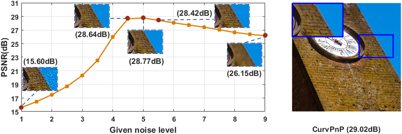
Figure 1: Image deblurring results of DPIR with different given noise levels (the left figure) and CurvPnP (the right image) on a blurry image with noise level 5.

In this paper, we propose a plug-and-play blind image restoration method with the deep curvature-based denoiser, called CurvPnP, which can ideally solve the blind noise removal problems by regarding the noise level as a variable. To be specific, we set up an effective two-stage blind denoising architecture, consisting of a noise estimation subnetwork and a denoising subnetwork, to deal with noisy images of different noise levels. The noise estimation subnetwork can calculate the noise level in each PnP iteration. Unlike the existing plug-and-play image restoration methods (Zhang et al, 2017c, 2022), which are designed for non-blind Gaussian denoising, our method does not need to know the noise level in advance. As illustrated in Fig. 1, the restoration performance of the state-of-the-art DPIR (Zhang et al, 2022) degraded obviously once the given noise level is inaccurate. Our CurvPnP can obtain high-quality restoration results without knowing the noise level in advance. The main contributions of this work are as follows

• We propose an effective and powerful two-stage blind image restoration method including the noise estimation subnetwork and denoising subnetwork, called C-UNet. In particular, we take the advantages of ConvNeXt block and encoder-decoder architecture to build up both subnetworks to maintain efficiency and improve model performance.

• We develop a novel denoiser containing rich curvature information, where Gaussian curvature map (Zhong et al, 2021) is not only used as a priori, but also used in the supervised attention module to refine the features. Thanks to the curvature information, our denoiser shows a strong ability to restore the edges and fine structures of images.

• The iterative PnP strategy is implemented for solving different image restoration problems such as image deblurring and super-resolution, where our CurvPnP is shown with very competitive results.

The rest of the paper is organized as follows. Sect. 2 dedicates to review the PnP image restoration methods. We describe the PnP blind image restoration method in Sect. 3. Sect. 4 introduces the deep curvature-based denoiser including the network architecture and implementation details. Experiments on three representative image restoration tasks are provided in Sect. 5. The concluding remarks and possible future works are summarized in Sect. 6.

2 Plug-and-play Image Restoration

The PnP priors were first proposed as denoisers for image restoration with traditional methods in Venkatakrishnan et al (2013). One of the most widely used denoisers for the plug-and-play framework is BM3D. Dar et al (2016) proposed a postprocessing method using the plug-and-play framework with BM3D as the denoiser for compression-artifact reduction. Rond et al (2016) introduced a plug-and-play prior for Poisson inverse problem (P⁴IP) with BM3D denoiser for image denoising and deblurring problems. Chan et al (2016) presented a continuation plug-and-play ADMM scheme, in which BM3D was used as a bounded prior for single image super-resolution and the single photon imaging problem. Ono (2017) plugged the BM3D as a Gaussian denoiser into the primal update for the primal-dual splitting (PDS) algorithm, whereas the dual update is devoted to handle with both data-fidelity term and hard constraint. Another widely used denoiser is the nonlocal mean (NLM) denoiser. Unni et al (2018) developed the linearized plug-and-play ADMM, where a fast low-complexity algorithm for doubly stochastic NLM was used as denoiser to deal with super-resolution and single-photon imaging. The weighted nuclear norm minimization (WNNM) (Gu et al, 2014) and Gaussian mixture model (GMM) (Zoran and Weiss, 2011) have also been implemented as denoiser. Kamilov et al (2017) proposed the fast iterative shrinkage thresholding algorithm with WNNM denoiser for nonlinear inverse scattering. Yair and Michaeli (2018) developed a variable splitting method to integrate WNNM denoiser for image inpainting and deblurring. Shi and Feng (2018) plugged the GMM denoiser into ADMM to solve the image restoration inverse problems. Teodoro et al (2019) built upon the plug-and-play framework by ADMM, and combined it with GMM as denoisers to address image deblurring, compressive sensing reconstruction, and super-resolution problem.

In recent years, the pre-trained deep learning denoisers are widely used for image restoration tasks. Zhang et al (2017a) decomposed the non-blind deconvolution problem into image denoising and image deconvolution and trained a fully connected CNN to remove noise. Meinhardt et al (2017) replaced the proximal operator of the regularization used in many convex energy minimization algorithms by a denoising neural network in exemplary problems of image deconvolution with different blur kernels and image demosaicking. Zhang et al (2017c) trained a set of denoisers for image denoising and plugged the learned denoiser prior into the optimization method to solve the image deblurring and super-resolution problems. Gu et al (2018) incorporated a CNN Gaussian denoiser prior and a non-local self-similarity based denoiser prior for image deblurring and super-resolution problems. Tirer and Giryes (2018) proposed an alternative method for solving inverse problems using off-the-shelf denoisers, which requires less parameter tuning. He et al (2019) plugged the residual CNNs into the ADMM algorithm to solve low-dose CT image reconstruction. Li and Wu (2019) plugged a set of CNN denoisers into the split Bregman iteration algorithm for solving the depth image inpainting problem. Zhang et al (2019b) proposed a principled formulation and framework by extending bicubic degradation based deep single image super-resolution with the PnP framework to recover the low-resolution images with arbitrary blur kernels. Dong et al (2019) implemented both the CNN based denoiser and the back-projection module to solve the super-resolution and deblurring tasks. Tirer and Giryes (2019) proposed the PnP iterative denoising and backward projection framework to image super-resolution using a set of CNN denoisers. Sun et al (2020) developed a block coordinate regularization-by denoising algorithm by leveraging the deep denoiser as the explicit regularizer. Bigdeli et al (2020) used the PnP CNN Maximum a Posteriori (MAP) denoiser to handle image denoising and inpainting tasks. By using the variable splitting technique, Zhao and Liang (2020) separated the fidelity term and regularization term and replaced the image prior model by learned prior implicitly for multi-frame super-resolution. Zheng et al (2021) proposed a neural network based method by combining with the deep Gaussian denoisers for image denoising. Zhang et al (2022) implicitly served a learning-based non-blind denoiser as the image prior for the PnP image deblurring, super-resolution and demosaicing methods. In Zhang and Timofte (2022), the deep PnP methods with a learning-based denoiser and deep unfolding methods are utilized to solve the image deblurring and super-resolution tasks. The theoretical convergence of the PnP scheme has been established under a certain Lipschitz condition on the denoisers in Ryu et al (2019). Bian et al (2021) solved the MRI reconstruction problem by applying meta-training on the adaptive learned regularization in the variational model. Wei et al (2020, 2022) presented the tuning-free PnP proximal algorithm, which can automatically determine the internal parameters such as the penalty parameter, the denoising strength and the terminal time.

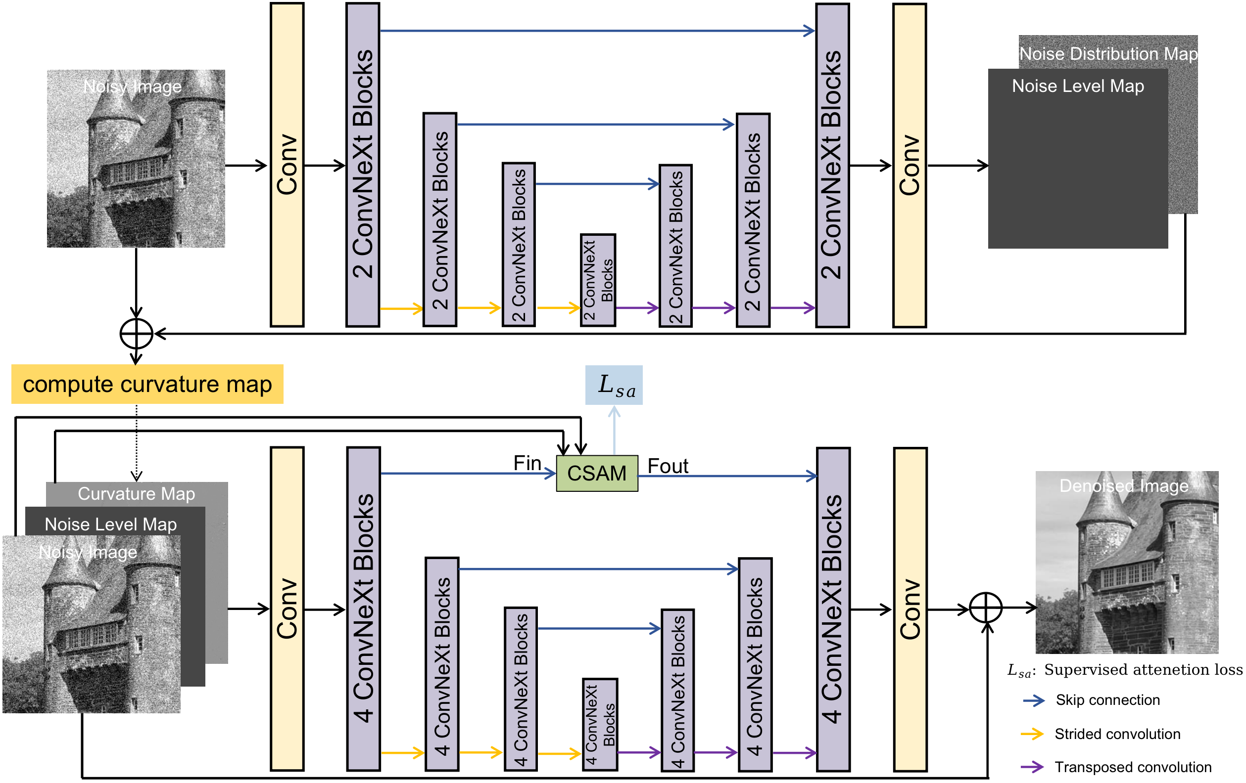
Figure 2: The proposed C-UNet for blind image denoising, which consists of a noise estimation subnetwork and a denoising subnetwork.

3 Plug-and-play Blind Image Restoration

As aforementioned, the up-to-date PnP method (Zhang et al, 2022) requires the noise level to be known, which is used to estimate the noise level for each iteration. However, once the noise level of the observed degraded image is inaccurate, the restoration result will be degraded obviously. For this, we propose a novel PnP framework by regarding the noise level as a variable. Firstly, to make the data fidelity and regularization separable, we introduce an auxiliary variable $v=x$ and rewrite the restoration model (3) into a constrained minimization problem as follows

$$\min_{x,v}~{}~{}\frac{1}{2\lambda\sigma_{s}^{2}}||y-\mathcal{T}(x)||^{2}+R(v)\quad s.t.\quad v=x,$$ (4)

where $\sigma_{s}$ denotes the noise level of the given degraded image $y$. We then reformulate it into the unconstrained minimization problem by the penalty method as follows

$$\min_{x,v,\sigma}~{}~{}\frac{1}{2\lambda\sigma_{s}^{2}}||y-\mathcal{T}(x)||^{2}+R(v)+\frac{1}{2\sigma^{2}}||v-x||^{2},$$ (5)

where $\sigma>0$ is a variable used to model the noise level of the noisy image $x$. Note that we introduce $\sigma$ to estimate the noise level that varies during iteration. In what follows, we sequentially minimize the two variables $x$ and $v$ iterative and alternatively by

$$x_{k+1}=\arg\min_{x}~{}~{}\frac{1}{2\lambda\sigma_{s}^{2}}||y-\mathcal{T}(x)||^{2}+\frac{1}{2\sigma_{k}^{2}}||v_{k}-x||^{2},$$ (6)

and

$$(\sigma_{k+1},v_{k+1})=\arg\min_{\sigma,v}~{}~{}\frac{1}{2\sigma^{2}}||v-x_{k+1}||^{2}+R(v),$$ (7)

respectively. More specifically, the sub-minimization problem (6) w.r.t. the data defility is a quadratic problem, which can be solved by the closed-form solution. The specific solution of $x$ depends on the degradation operator $\mathcal{T}$, which will be given in the experiment section. On the other hand, the solution of (7) corresponds to the Gaussian denoising problem with the noise level $\sigma$. Obviously, the noise level $\sigma$ varies in the PnP iteration scheme. Unlike the existing Gaussian denoiser, the noise level $\sigma$ should be given in advances. We regard the noise level $\sigma$ as a variable and estimate it by the latest recovered image $x_{k+1}$ as follows

$$\sigma_{k+1}=Noise\_Estimator(x_{k+1}),$$ (8)

which is realized by a convolutional neural network.

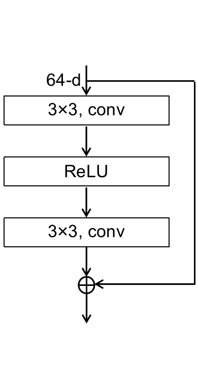
(a) ResNet Block in Zhang et al (2022)

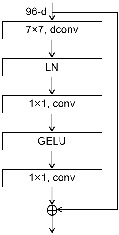
(b) ConvNeXt Block in Liu et al (2022b)

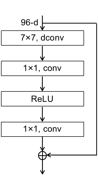
(c) ConvNeXt Block in C-UNet

Figure 3: The block design for the ResNet in Zhang et al (2022), the ConvNeXt in Liu et al (2022b) and the ConvNeXt used in our network model.

Now, we can solve the variable $v$ by a certain denoiser. Since the noise distribution varies across different image restoration tasks, we introduce an artificial noise control parameter $\rho$ as the coefficient of noise level map to reduce the influence of degenerate operations on noise distribution. Considering that the curvature map contains plentiful image details, we take curvature as a priori, and estimate the solution $v_{k+1}$ from

$$v_{k+1}=Denoiser(x_{k+1},\rho\sigma_{k+1},c_{k+1}),$$ (9)

which is a convolutional neural network called the deep curvature denoiser.

Based on the above discussion, we come up with the PnP blind image restoration method with deep curvature denoiser (shorted by CurvPnP); see Algorithm 1.

Algorithm 1 CurvPnP: Plug-and-play blind image restoration with deep curvature denoisier

Input: Original image $y$, degradation operator $\mathcal{T}$ and positive constants $\lambda$ and $\rho$;

Initialize: $\sigma_{s}=Noise\_Estimator(y)$, $\sigma_{0}=50$ and $v_{0}=y$;

for $k=0,1,\dots,K-1$ do

  (i)   Compute $x_{k+1}$ from (6);

  (ii)  Compute $\sigma_{k+1}$ from (8);

  (iii) Compute $v_{k+1}$ from (9);

  (iv) Check whether the following stopping condition is satisfied:

     PSNR($v_{k+1}$)$<$PSNR($v_{k}$);

end for

Output: $v$

4 Deep Curvature Denoiser

4.1 Network Architecture

C-UNet. The encoder-decoder architecture (Zamir et al, 2021) is well-known for its strong ability in encoding contextual information. However, the classical encoder-decoder UNet lacks the capability to preserve spatial image details and texture structure. Thus, the proposed denoiser, namely C-UNet, integrates the curvature map into UNet for effective denoiser prior modeling. Our C-UNet consists of two subnetworks, i.e., the noise estimation subnetwork and denoising subnetwork, to solve the sub-minimization problem w.r.t. $\sigma$ and $v$, respectively. As illustrated in Fig. 2, both subnetworks are built up using UNet architecture. In particular, the noise estimation subnetwork takes the noisy image $x$ as the input to obtain both the noise level map and noise distribution map. Then we calculate the Gaussian curvature map (Zhong et al, 2021) based on the estimated clean image obtained by removing the noise distribution map from the noisy input. The reason why we choose Gaussian curvature map as a priori is that Gaussian curvature is more suitable for real images in preserving fine structures and details (Zhong et al, 2021). The denoising subnetwork takes the noisy image, the noise level map and Gaussian curvature map as the input. Similar to Zhang et al (2022), we build up the noise estimation subnetwork and denoising subnetwork based on the encoder-decoder architecture by the 2$\times$2 stride convolution and 2$\times$2 transposed convolution in downsampling and upsampling operations, respectively. Besides, both the ConvNeXt blocks and curvature supervised attention module are introduced for effective denoiser prior modeling.

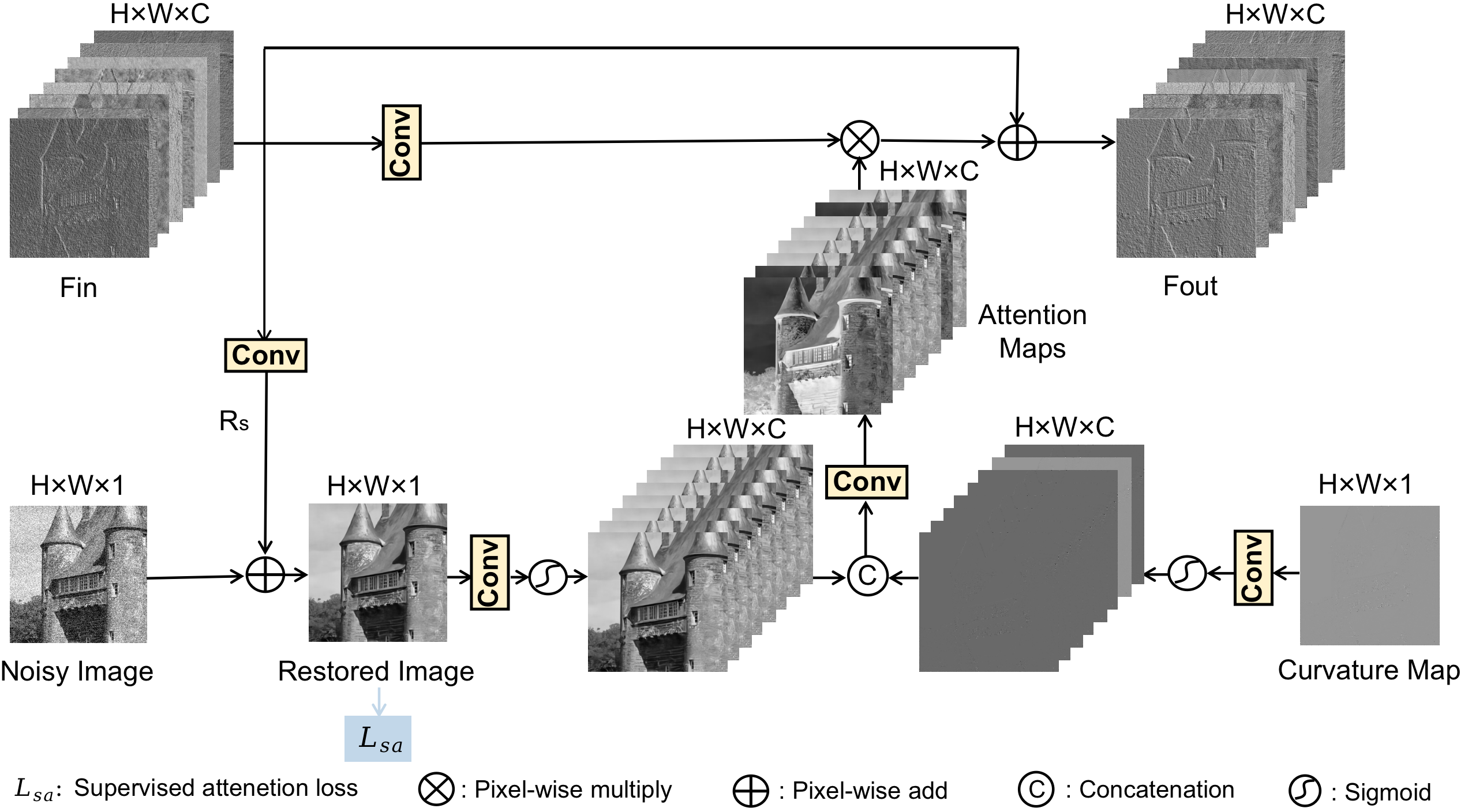
Figure 4: The proposed curvature supervised attention module (CSAM).

ConvNeXt Block. Inspired by Liu et al (2022b), we integrate the ConvNeXt blocks into UNet for both the noise estimation and denoising subnetworks to promote the ability in feature extraction. Different from the ResNet block (Fig. 3 (a)) used in DRUNet (Zhang et al, 2022), ConvNeXt block (Fig. 3 (b)) takes the advantage of the depthwise convolution and expand the network width from 64 to 96 to increase the diversity of features. In addition, the inverted bottleneck is used to avoid loss of information and the large depthwise convolution with kernel size 7$\times$7 is used to improve the performance. In our implementation, we remove the layer normalization and use ReLU to replace GELU to save the memory and raise the effectiveness; see Fig. 3 (c).

Curvature Supervised Attention Module. The supervised attention module is shown capable to enrich the features in the multi-stage progressive image restoration (Zamir et al, 2021). Proceeding from the same purpose, we propose a Curvature Supervised Attention Module (CSAM) in the denoising subnetwork. Fig. 4 illustrates the schematic diagram of CSAM, where the curvature map is integrated with the attention maps to enhance the useful features. We use a $1\times 1$ convolution to the curvature map followed by the sigmoid activation, which are then integrated with the feature maps obtained by restored images to produce the attention maps through $1\times 1$ convolution. By introducing CSAM, the useful features can propagate to the decoder and the less informative features are suppressed by the attention masks.

4.2 Implementation Details

For a fair comparison with DRUNet (Zhang et al, 2022), we use the same training dataset, which consists of 4744 images of Waterloo Exploration Database (Ma et al, 2017), 900 images from DIV2K dataset (Agustsson and Timofte, 2017) and 2650 images from Flick2K dataset (Lim et al, 2017). Note that 400 Berkeley segmentation dataset (BSD) is not included because the images of size 180$\times$180 are too small to fit the large training patch size. In order to use a single model to handle noisy image of different noise levels, the noise level of the training data is randomly selected from the range $[0,50]$.

For the noise estimation subnetwork, we set the initial learning rate as 2e-4 and decrease it by half every 60000 iterations until reaching 1.25e-5. The patch size and batch size are fixed as 256$\times$256 and 64, respectively. The Adam optimizer is used to optimize the noise estimation subnetwork end-to-end with the following loss function

$$L_{N}=||X_{NL}-\hat{X}_{NL}||_{1}+||X_{ND}-\hat{X}_{ND}||_{1},$$ (10)

where $X_{NL}$ and $\hat{X}_{NL}$ denotes the estimated noise level map and the corresponding ground truth, $X_{ND}$ and $\hat{X}_{ND}$ represents the predicted noise distribution map and its ground truth, respectively.

For the denoising subnetwork, the learning rate starts from 2e-4 and decays by a factor of 0.5 every 100000 iterations and finally ends once it is smaller than 2.5e-5. The denoisier network is trained on 224$\times$224 patches with a batch size of 24. The parameters are also optimized by Adam optimizer by the following loss function

$$L_{I}=||X-\hat{X}||_{1}+L_{sa},$$ (11)

where $X$ and $\hat{X}$ are the denoised image the corresponding ground-truth image, and $L_{sa}$ is supervised attention loss defined as

$$L_{sa}=||X_{S}-\hat{X}||_{1},$$ (12)

with $X_{S}$ being the restored image in CSAM. The number of channels in each layer from the first scale to the fourth scale are set as 96, 192, 384 and 768 for both noise estimation and denoising subnetworks. It takes about twenty hours and three days twelve hours to train the noise estimation subnetwork and denoising subnetwork on four NVIDIA Geforce RTX 3090 GPUs, respectively.

5 Experiments

In this section, we evaluate the performance of our CurvPnP on three representative image restoration tasks including gray/color image denoising, deblurring and super-resolution. All traditional restoration methods (including BM3D (Dabov et al, 2007) and TFOV (Yao et al, 2020)) are run on an Intel Core i7 CPU at 3.60GHz, while the learning based methods (including NN+BM3D (Zheng et al, 2021), IRCNN (Zhang et al, 2017c), CBDNet (Guo et al, 2019), FDnCNN (Zhang et al, 2017b), DRUNet (Zhang et al, 2022), C-UNet, DMPHN (Zhang et al, 2019a), MPRNet (Zamir et al, 2021), DWDN (Dong et al, 2020), ZSSR (Shocher et al, 2018), SRFBN (Li et al, 2019), DPIR (Zhang et al, 2022), DPIR+ and CurvPnP) are implemented on a NVIDIA Geforce RTX 3090 GPU.

5.1 Datasets

We perform evaluation on various testing datasets, including Set9 (Ulyanov et al, 2018), Kodak24 (Franzen, 1999), Urban100 (Huang et al, 2015), PIPAL (Gu et al, 2020), CC (Nam et al, 2016) and PolyU (Xu et al, 2018) dataset. The Set9 dataset contains 9 classic color images with size of 512$\times$512 or 768$\times$512; the Kodak24 dataset includes 24 color images with size of 500$\times$500; the Urban100 dataset has 100 images of urban scenes of different sizes; the PIPAL dataset contains 200 images of size 288$\times$288; both CC and PolyU datasets are with 15 and 100 images of size 512$\times$ 512.

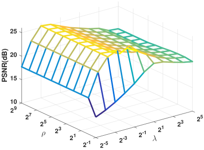
Figure 5: The PSNR evolutions of $Church$ in Fig. 10 obtained by different combinations of the parameters $\lambda$ and $\rho$.

Noisy Image

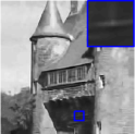
BM3D (24.28dB)

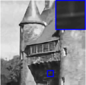
NN+BM3D (24.33dB)

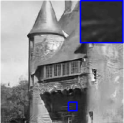
IRCNN (24.88dB)

FDnCNN (24.92dB)

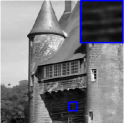
DRUNet (25.27dB)

C-UNet (25.33dB)

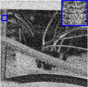
Noisy Image

BM3D (28.49dB)

NN+BM3D (29.16dB)

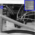
IRCNN (30.54dB)

FDnCNN (30.92dB)

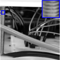
DRUNet (32.89dB)

C-UNet (33.17dB)

Figure 6: Grayscale image denoising results of different methods on the image “A0025” from PIPAL dataset and image “Canon5D2_5_160_6400_circuit_11” from PolyU dataset with noise level of 50.

Table 1: Average PSNR(dB)/SSIM results of different methods with noise levels 20, 35 and 50 for grayscale image denoising on Set9, Urban100, PIPAL, CC and PolyU datasets. The best and second best scores are highlighted and underline, respectively.

Datasets	$\sigma_{s}$	BM3D	NN+BM3D	IRCNN	FDnCNN	DRUNet	C-UNet
Set9	20	31.73/0.8498	31.70/0.8501	32.11/0.8550	32.20/0.8601	32.60/0.8703	32.64/0.8710
	35	29.32/0.7851	29.08/0.7863	29.84/0.8033	29.90/0.8059	30.41/0.8215	30.46/0.8221
	50	27.59/0.7347	27.65/0.7382	28.36/0.7620	28.45/0.7660	29.08/0.7877	29.15/0.7887
Urban100	20	30.54/0.8878	30.48/0.8872	30.95/0.9014	31.25/0.9080	32.12/0.9222	32.18/0.9223
	35	27.21/0.8151	27.11/0.8153	28.11/0.8453	28.38/0.8519	29.58/0.8825	29.69/0.8841
	50	24.83/0.7465	24.79/0.7485	26.23/0.7919	26.52/0.8011	27.96/0.8483	28.12/0.8517
PIPAL	20	29.41/0.8811	29.37/0.8802	29.92/0.8859	30.04/0.8900	30.42/0.8985	30.49/0.8998
	35	26.33/0.7923	26.35/0.7989	27.08/0.8133	27.20/0.8171	27.66/0.8340	27.74/0.8369
	50	24.29/0.7138	24.43/0.7251	25.37/0.7507	25.49/0.7557	26.00/0.7806	26.10/0.7851
CC	20	36.74/0.9399	36.69/0.9407	37.30/0.9477	37.58/0.9503	38.57/0.9567	38.73/0.9575
	35	33.08/0.8981	32.80/0.8985	34.22/0.9159	34.57/0.9216	35.89/0.9345	36.09/0.9358
	50	30.22/0.8585	30.16/0.8581	32.17/0.8832	32.61/0.8964	34.10/0.9159	34.36/0.9180
PolyU	20	37.83/0.9474	37.76/0.9479	38.81/0.9593	39.11/0.9614	40.43/0.9698	40.56/0.9703
	35	33.94/0.9093	33.57/0.9088	35.94/0.9375	36.29/0.9422	38.05/0.9577	38.26/0.9590
	50	30.84/0.8747	30.65/0.8742	33.87/0.9138	34.36/0.9253	36.37/0.9473	36.62/0.9491

5.2 Parameter Selection

There are two parameters in our model, i.e., the regularization parameter $\lambda$ and noise level control parameter $\rho$. Our method is not sensitive to the choices of $\lambda$, which is fixed as $\lambda=0.37$ for image deblurring and super-resolution tasks. Because the noise distribution changes with different image restoration tasks, the value of $\rho$ varies for different degradation operations. We choose $\rho=1.2$ for image deblurring and $\rho=5$, $25$ and $50$ for SISR with scale factor $2$, $3$ and $4$, respectively. For both image deblurring and super-resolution tasks, the maximum iteration number $K$ is set to 15. Fig. 5 displays the PSNR results on image $Church$ from PIPAL dataset in Fig. 10 with different combinations of $\lambda$ and $\rho$, where $\lambda$ and $\rho$ are chosen from $(\lambda,\rho)\in\{2^{-5},2^{-4},\ldots,2^{5}\}\times\{2^{-1},2^{0},\ldots,2^{9}\}$. As shown, PSNR values are relatively stable such that there are reasonably large internals for parameters to generate good restoration results. Note that $\rho$ should be chosen larger than $1$ to obtain high quality restoration results.

5.3 Image Denoising

Table 2: Average PSNR(dB)/SSIM results of different methods with noise levels 20, 35 and 50 for color image denoising on Kodak24, Urban100, PIPAL, CC and PolyU datasets. The best and second best scores are highlighted and underline, respectively.

Datasets	$\sigma_{s}$	BM3D	NN+BM3D	IRCNN	CBDNet	FDnCNN	DRUNet	C-UNet
Kodak24	20	30.53/0.8912	30.51/0.8913	33.08/0.8956	33.10/0.8965	33.20/0.8995	33.83/0.9094	33.89/0.9102
	35	29.46/0.8190	29.49/0.8232	30.43/0.8386	30.45/0.8371	30.57/0.8423	31.28/0.8599	31.36/0.8614
	50	27.28/0.7579	27.47/0.7652	28.81/0.7932	28.85/0.7894	28.97/0.7965	29.74/0.8202	29.82/0.8224
Urban100	20	31.97/0.9081	31.92/0.9075	32.30/0.9222	32.28/0.9226	32.57/0.9275	33.56/0.9385	33.63/0.9392
	35	28.55/0.8541	28.52/0.8519	29.49/0.8788	29.59/0.8784	29.87/0.8862	31.15/0.9088	31.27/0.9103
	50	25.96/0.8008	26.09/0.8003	27.70/0.8393	27.85/0.8381	28.10/0.8482	29.61/0.8832	29.76/0.8857
PIPAL	20	31.17/0.9149	31.18/0.9151	31.72/0.9211	31.73/0.9213	31.89/0.9241	32.48/0.9323	32.56/0.9332
	35	27.85/0.8479	27.98/0.8547	28.83/0.8673	28.89/0.8670	29.02/0.8720	29.69/0.8871	29.79/0.8890
	50	25.45/0.7807	25.75/0.7937	27.08/0.8199	27.13/0.8180	27.26/0.8252	27.98/0.8470	28.09/0.8499
CC	20	36.89/0.9276	36.87/0.9284	37.92/0.9552	38.27/0.9549	38.52/0.9571	39.92/0.9663	40.10/0.9672
	35	32.55/0.8843	32.77/0.8882	35.10/0.9266	35.33/0.9267	35.58/0.9319	37.34/0.9486	37.57/0.9500
	50	29.24/0.8434	29.42/0.8465	33.13/0.8978	33.36/0.8993	33.65/0.9086	35.63/0.9332	35.91/0.9353
PolyU	20	38.55/0.9492	38.59/0.9502	39.49/0.9638	39.82/0.9644	40.07/0.9663	41.21/0.9724	41.35/0.9729
	35	34.17/0.9139	34.53/0.9179	36.98/0.9440	37.12/0.9457	37.45/0.9496	39.19/0.9624	39.38/0.9634
	50	30.65/0.8811	31.19/0.8864	34.96/0.9249	35.22/0.9280	35.63/0.9347	37.78/0.9539	38.02/0.9556

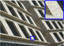
Noisy Image

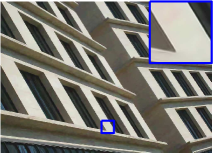
BM3D (29.06dB)

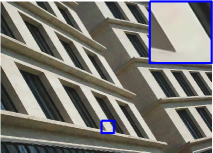
NN+BM3D (29.30dB)

IRCNN (30.44dB)

CBDNet (30.80dB)

FDnCNN (30.99dB)

DRUNet (32.96dB)

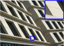
C-UNet (33.25dB)

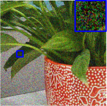
Noisy Image

BM3D (27.92dB)

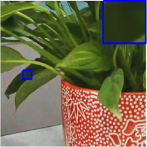
NN+BM3D (28.26dB)

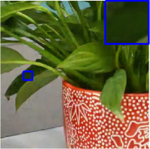
IRCNN (29.93dB)

CBDNet (30.19dB)

FDnCNN (30.30dB)

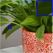
DRUNet (31.86dB)

C-UNet (32.06dB)

Figure 7: Color image denoising results of different methods on the image “img025” from Urban100 dataset and image “Sony_4-5_125_3200_plant_10”from PolyU dataset with noise level of 50.

5.3.1 Comparison methods

We compare the proposed C-UNet with the well-known traditional and learning-based denosing methods, the details of which are summarized as follows

• BM3D (Dabov et al, 2007): The Block Matching and 3D filtering (BM3D) is an image denoising method which integrates 3-D transformation of a group, shrinkage of the transform spectrum and inverse 3-D transformation and demands the noise level as input.

• NN+BM3D (Zheng et al, 2021): The unsupervised denoising method NN+BM3D combines the encoder-decoder convolutional neural network with the Gaussian denoiser BM3D, which does not require any training samples, but needs the noise level as the input.

• IRCNN (Zhang et al, 2017c): The Image Restoration Convolutional Neural Network (IRCNN) involves 25 separate 7-layer denoisers, which were trained on a certain noise level from the range of [0, 50]. The training dataset consists of 400 BSD images, 400 selected ImageNet database images and 4744 Waterloo Exploration Database images.

• CBDNet (Guo et al, 2019): The Convolutional Blind Denoising Network (CBDNet) model includes a noise estimation sub-network to obtain the noise level map and a non-blind denoising subnetwork to estimate the denoising results. For a fair comparison, we retrained the CBDNet using the same training dataset as ours, i.e., 4744 Waterloo Exploration Database, 900 DIV2K and 2650 Flick2K images corrupted by additive Gaussian noises of noise level [0, 50].

• FDnCNN (Zhang et al, 2017b): By taking a noise level map as input, the Flexible Denoising Convolutional Neural Network (FDnCNN) was trained on 400 BSD images corrupted by Gaussian noises with noise level ranging form 0 to 75.

• DRUNet (Zhang et al, 2022): The Denoising Residual block based U-Net (DRUNet) adopts the U-Net architecture with ResNet blocks, which takes the noise level map as input. It was trained on BSD400, Waterloo Exploration Database, DIV2K and Flick2K datasets degraded by random Gaussian noises of level [0, 50].

5.3.2 Quantitative and qualitative comparison results

Table 1 presents the grayscale image denoising results of the noise level $\sigma_{s}=20$, $35$ and $50$ on different datasets. As shown, our C-UNet achieves the best restoration results for all datasets, especially for images with big noises. The visual comparisions on the images “A0025” from PIPAL dataset and “Canon5D2_5_160_6400_circuit_11” from PolyU dataset with noise level $\sigma_{s}=50$ are displayed in Fig. 6. As can be observed by the magnified portions, our C-UNet is very effective in preserving edges and texture structures. Concretely speaking, our C-UNet can preserve the texture of the wall and the fringe of the device.

Similarly, we conduct the comparison experiments on color image restoration problems. The denoising results on different datasets are presented in Table 2. Once again, we observe that our C-UNet gives the best performance for all noise levels, which demonstrate the superiority of our C-UNet in dealing with noises in a wide range. Fig. 7 shows the visual results of different methods on the images “img025” from Urban100 dataset and “Sony_4-5_125_3200_plant_10” from PolyU dataset with noise level $\sigma_{s}=50$. It can be observed that BM3D, NN+BM3D, IRCNN, CBDNet, FDnCNN and DRUNet can remove the noises but cannot recover the sharp structures of images. Obviously, our C-UNet performs better in preserving fine structures such as the stripes on the wall and the leaf vein, proving the effect of the curvature information.

Table 3: Average runtime comparison (in seconds) among different methods on color image denoising datasets.

Datasets	BM3D	NN+BM3D	IRCNN	CBDNet	FDnCNN	DRUNet	C-UNet
Kodak24	7.3183	1134.26	0.0383	0.0472	0.1846	0.0867	0.3417
Urban100	23.0133	1468.20	0.1153	0.1159	0.5239	0.2660	1.2084
PIPAL	2.3057	949.20	0.0144	0.0161	0.0712	0.0462	0.1190
CC	7.9339	1238.95	0.0437	0.0499	0.1887	0.1063	0.3844
PolyU	8.1621	1218.75	0.0387	0.0458	0.1849	0.1015	0.4055

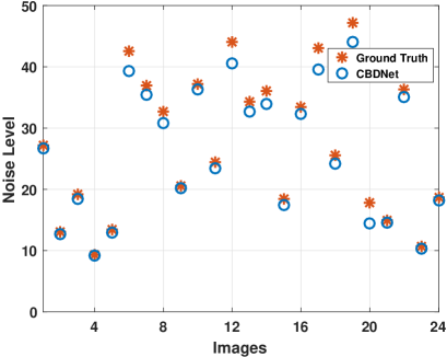
(a) CBDNet

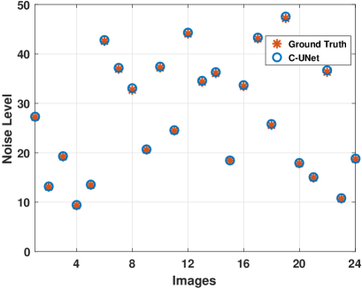
(b) C-UNet

Figure 8: The noise level obtained by CBDNet and C-UNet on Kodak24 dataset, which are degraded by random Gaussian noises of level $\sigma\in[0,50]$.

5.3.3 Computational efficiency

Table 3 reports the comparison results on the average run time of the aforementioned denoising methods on color image datasets with noise level 50. Compared with CBDNet, IRCNN, FDnCNN and DRUNet, although our C-UNet consumes a little bit more time due to the curvature map, it provides much better PSNR values. Note that the unsupervised NN+BM3D costs the most computational time due to the on-line learning strategy.

5.3.4 Noise estimation

To verify the accuracy of the noise estimation subnetwork in our C-UNet, we compare the noise levels obtained by CBDNet and C-UNet on Kodak24 dataset, where the test images are corrupted by Gaussian noises of noise level $\sigma_{s}\in[0,50]$. As can be observed in Fig. 8, the noise levels estimated by our C-UNet are close to the truth noise levels added into the test images. Since the noise estimation sub-network of CBDNet adopts a five-layer plain fully connected convolutional network, which does not work as powerful as the UNet used in our C-UNet, it tends to underestimate the noise levels and the performance is also not as stable as ours.

5.4 Image Deblurring

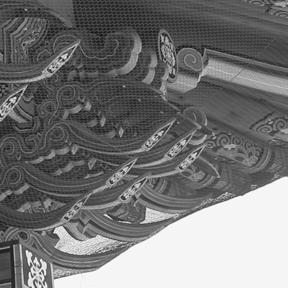
(a) Eave

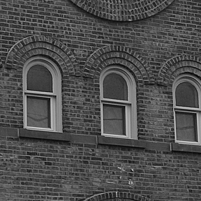
(b) Wall

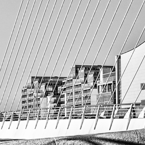
(c) Bridge

(d) Sign

(e) Branch

(f) Glass

(g) Woman

(h) House

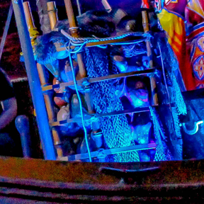
(i) Blue

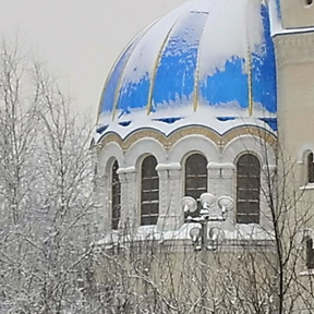
(j) Church

Figure 9: Ten test images for image deblurring experiments.

The degradation model of the blurry observation $y$ can be described by

$$y=Ax+n,$$ (13)

where $Ax$ denotes the convolution of the clean image $x$ with the blur operator $A$.

Our CurvPnP method focuses on the non-blind deblurring with the blur kernel being assumed known. For image deblurring, the $x$ subproblem (6) can be defined as follows

$$x_{k+1}=\arg\min_{x}~{}\frac{1}{2\lambda\sigma_{s}^{2}}||y-Ax||^{2}+\frac{1}{\sigma_{k}^{2}}||v_{k}-x||^{2},$$ (14)

the Euler-Lagrange equation of which gives

$$(\sigma_{k}^{2}A^{*}A+\lambda\sigma_{s}^{2}\mathcal{I})x_{k+1}=\sigma_{k}^{2}A^{*}y+\lambda\sigma_{s}^{2}v_{k},$$ (15)

with $A^{*}$ being the adjoint of $A$ and $\mathcal{I}$ being the identity operator. The above equation can be efficiently solved by the discrete fast Fourier transform (FFT), that is

$$x_{k+1}=\mathcal{F}^{-1}\Bigg{(}\frac{\sigma_{k}^{2}\overline{\mathcal{F}(A)}\mathcal{F}(y)+\lambda\sigma_{s}^{2}\mathcal{F}(v_{k})}{\sigma_{k}^{2}\overline{\mathcal{F}(A)}\mathcal{F}(A)+\lambda\sigma_{s}^{2}\mathcal{I}}\Bigg{)}.$$ (16)

5.4.1 Comparison methods

We compare the deblurring results of our CurvPnP with several state-of-the-art deblurring approaches, including the learning-based blind methods, non-blind method DWDN and PnP approaches. The details of deblurring methods are expressed as follows

• DMPHN (Zhang et al, 2019a): The Deep Multi-Patch Hierarchical Network (DMPHN) deals with blurry images via a fine-to-coarse hierarchical representation. The DMPHN was trained on the dataset consists of 2103 image pairs of GoPro dataset and 61 videos from VideoDeblurring dataset.

• MPRNet (Zamir et al, 2021): The Multi-stage Progressive Restoration Network (MPRNet) model injects supervision at each stage to progressively improve degraded inputs. It was trained end-to-end on 2103 image pairs from GoPro dataset.

• DWDN (Dong et al, 2020): The Deep Wiener Deconvolution Network (DWDN) is a domain-specific network that integrates the feature-based Wiener deconvolution into a deep neural network for non-blind image deblurring. It was trained on BSD400 and 4744 Waterloo Exploration datasets with synthetic realistic blur kernels of random sizes in the range from 13$\times$13 to 15$\times$15 pixels and Gaussian noises with noise levels in between [0, 12.75].

• IRCNN (Zhang et al, 2017c): It is a CNN denoiser prior based PnP image restoration method, for which the number of iteration was fixed as 30 for image deblurring problems.

• DPIR (Zhang et al, 2022): The Deep PnP Image Restoration (DPIR) is built up in the PnP framework using DRUNet as the denoiser, for which the iteration number of is fixed as 8 for image deblurring problems.

• DPIR+: We introduce the noise estimation method (Chen et al, 2015) into the denoiser DRUNet for dealing with the blind image restoration problem, which is shorted as DPIR+.

Table 4: PSNR(dB) results of different methods for image deblurring on GSet5 and CSet5 datasets. The best and second best scores are highlighted and underline, respectively.

Kernel	$\sigma_{s}$	Methods	Eave	Wall	Bridge	Sign	Branch	Glass	Woman	House	Blue	Church
First	4	DMPHN	19.88	18.62	16.39	17.99	16.97	20.30	13.73	16.63	18.52	14.84
(19$\times$19)		MPRNet	-	-	-	-	-	22.87	15.80	18.61	19.37	17.64
		DWDN	-	-	-	-	-	31.79	25.07	30.31	25.80	27.55
		IRCNN	28.08	26.00	27.69	28.87	29.47	34.86	27.33	31.26	28.22	28.57
		DPIR	28.70	27.42	28.65	29.98	29.89	36.26	28.75	32.26	29.09	29.34
		DPIR+	28.43	26.63	27.72	29.99	28.53	36.26	28.43	32.27	29.19	29.26
		CurvPnP	28.88	27.56	28.67	30.12	30.23	36.67	29.09	32.33	29.30	29.36
	8	DMPHN	19.03	17.74	15.57	17.96	16.92	19.71	13.80	16.20	18.26	14.82
		MPRNet	-	-	-	-	-	21.55	16.46	17.62	18.89	16.54
		DWDN	-	-	-	-	-	30.18	23.77	28.13	24.32	25.27
		IRCNN	26.05	23.40	24.34	25.56	26.24	32.33	23.85	28.48	25.67	25.72
		DPIR	26.42	24.68	25.35	27.08	26.25	33.18	25.96	29.32	26.31	26.17
		DPIR+	26.49	24.67	25.06	27.06	26.04	32.55	25.78	29.37	26.37	26.26
		CurvPnP	26.56	25.09	25.62	27.13	26.64	33.89	26.60	29.63	26.71	26.52
Fourth	4	DMPHN	17.62	18.26	13.56	13.64	12.68	14.14	14.33	17.66	13.71	15.37
(27$\times$27)		MPRNet	-	-	-	-	-	14.32	14.57	17.82	13.64	16.54
		DWDN	-	-	-	-	-	29.46	23.54	28.40	23.62	26.04
		IRCNN	27.60	25.78	26.98	28.32	28.68	34.60	26.71	30.62	27.85	27.85
		DPIR	28.24	27.00	28.08	29.51	28.95	35.91	28.06	31.65	28.56	28.70
		DPIR+	28.08	26.86	27.64	29.55	27.77	35.77	27.98	31.56	28.59	28.60
		CurvPnP	28.36	27.22	28.14	29.72	29.19	36.29	28.60	31.71	28.82	28.76
	8	DMPHN	17.02	17.50	13.17	13.39	12.82	13.40	13.77	16.24	13.37	14.85
		MPRNet	-	-	-	-	-	13.95	14.35	17.00	12.91	16.18
		DWDN	-	-	-	-	-	28.52	22.14	26.70	22.54	24.27
		IRCNN	25.53	22.66	23.61	24.86	25.29	32.05	23.33	27.72	25.29	25.17
		DPIR	25.81	24.28	24.77	26.47	25.27	33.12	25.26	28.68	25.85	25.55
		DPIR+	25.98	24.30	24.77	26.48	24.91	32.46	25.32	28.73	25.88	25.69
		CurvPnP	26.08	24.92	25.14	26.88	25.90	33.62	26.06	28.99	26.29	25.93

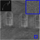
Blurry Image

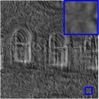
DMPHN (17.50dB)

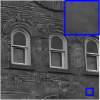
IRCNN (22.66dB)

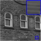
DPIR (24.28dB)

DPIR+ (24.30dB)

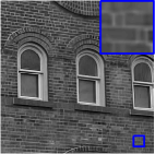
CurvPnP (24.92dB)

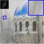
Blurry Image

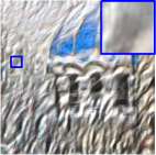
DMPHN (14.82dB)

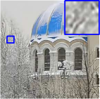
IRCNN (25.72dB)

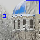
DPIR (26.17dB)

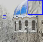
DPIR+ (26.26dB)

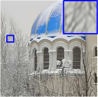
CurvPnP (26.52dB)

Figure 10: Image deblurring results of different methods on the image “Wall” and “Church” with noise level of 8. The blur kernels are shown on the upper left corner of the blurry images.

Table 5: Average runtime comparison (in seconds) among different methods on image deblurring datasets.

Datasets	DMPHN	DWDN	MPRNet	IRCNN	DPIR	DPIR+	CurvPnP
GSet5	0.0707	-	-	0.0992	0.1442	0.1874	0.4490
CSet5	0.0782	0.3721	0.1184	0.1350	0.1844	0.4416	0.9762

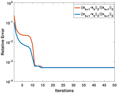
(a) Relative Error

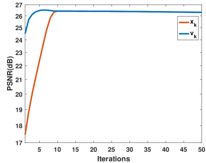
(b) PSNR

Figure 11: The evolution of relative errors $\frac{\|x_{k+1}-x_{k}\|_{2}}{\|x_{k+1}\|_{2}}$ and $\frac{\|v_{k+1}-v_{k}\|_{2}}{\|v_{k+1}\|_{2}}$ and PSNR via iterations for the image “Church” in Fig. 10.

5.4.2 Quantitative and qualitative comparison

We choose ten testing images including five grayscale images (GSet5) and five color images (CSet5), for image deblurring experiments; see Fig. 9. We quantitatively evaluate our method on the dataset with two real blur kernels of size $19\times 19$ and $27\times 27$ from Levin et al (2009) and additive Gaussian noises of noise levels 4 and 8, respectively.

In Table 4, it can be seen that our proposal is more stable and robust against different blur kernels and noises for both grayscale and color images. Since DMPHN and MPRNet are blind deblurring methods, they are not as powerful as other learning-based methods in removing the blurry contained in the images. More importantly, our CurvPnP outperforms the available most effective method DPIR by an average PSNR of 0.16dB$\sim$0.46dB on grayscale images and 0.21dB$\sim$0.49dB on color images. Note that the DPIR requires the ground truth noise level. When the noise level is approximated by the estimation method (Chen et al, 2015), the performance of the DPIR+ drop to a certain degree for some test images.

Fig. 10 illustrates the deblurring results on the images “Wall” and “Church”. As shown by both visual and quantitative results, DMPHN cannot handle the distortion of blur, while the IRCNN, DPIR and DPIR+ tend to smooth out the edges and details. Instead, the images restored by our CurvPnP are much sharper and closer to the ground-truth. Specifically, our CurvPnP can yield the crotch of the tree for the image “Church”, while other methods fail to provide the clear structures.

5.4.3 Computational efficiency and numerical convergence

In Table 5, we record the average running time of different restoration methods on image deblurring datasets with the first blur kernel and noise level 8. Although our CurvPnP is somehow slower than other learning based methods, the computational speed is still acceptable for consuming less than second to process a color image of size 288 $\times$ 288.

Fig. 11 records the evolution of both the relative errors and PSNR on the image “Church” in Fig. 10 by 50 iterations for our CurvPnP method. Although the relative error curves vibrate at the beginning, they all converge to zero as the iteration number keeps increasing in Fig. 11 (a). Fig. 11 (b) also demonstrate that both PNSR of $x_{k}$ and $v_{k}$ converge quickly. As can be seen, since $v$ is the clean image estimated by the denoiser, it converges faster than $x$, and the two variables converge to the same steady values.

5.5 Single Image Super-Resolution

Table 6: Average PSNR(dB) results of different methods for single image super-resolution on CC and PolyU datasets. The best and second best scores are highlighted and underline, respectively.

Datasets	Scale	$\sigma_{s}$	Channel	TFOV	ZSSR	SRFBN	IRCNN	DPIR	DPIR+	CurvPnP
CC	$\times$2	8	RGB	29.63	26.90	26.99	33.56	39.97	38.73	40.11
			Y	33.11	30.89	30.93	36.55	41.98	41.06	42.08
	$\times$2	16	RGB	24.72	21.71	21.66	30.66	37.15	36.09	37.44
			Y	28.89	26.05	25.97	33.41	39.25	38.86	39.48
	$\times$3	4	RGB	33.95	32.56	32.87	32.30	35.11	35.22	35.68
			Y	37.04	36.19	36.50	36.66	36.77	37.03	37.37
	$\times$4	8	RGB	28.18	26.94	27.29	26.53	30.46	29.96	32.13
			Y	31.74	30.73	31.27	30.87	32.20	32.52	33.88
PolyU	$\times$2	8	RGB	29.75	27.03	27.03	33.56	40.82	40.12	40.88
			Y	33.39	31.08	31.14	36.53	42.88	42.29	42.91
	$\times$2	16	RGB	24.70	21.68	21.64	31.04	38.78	37.92	38.97
			Y	29.00	26.16	26.09	33.77	40.87	40.13	41.04
	$\times$3	4	RGB	33.84	32.56	32.36	32.22	36.75	36.41	37.04
			Y	37.05	36.34	35.91	36.62	38.33	38.34	38.67
	$\times$4	8	RGB	28.29	26.98	27.35	26.59	32.48	30.54	33.41
			Y	32.08	30.91	31.55	31.06	34.02	33.48	35.32

Low-resolution Image

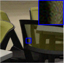
TFOV (26.29dB)

ZSSR (24.79dB)

SRFBN (23.68dB)

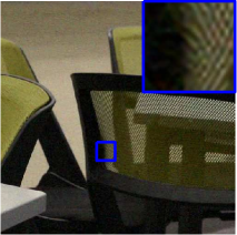
IRCNN (27.88dB)

DPIR (32.31dB)

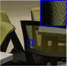
DPIR+ (32.51dB)

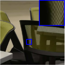
CurvPnP (32.82dB)

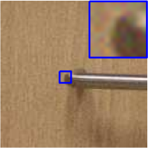
Low-resolution Image

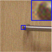
TFOV (28.94dB)

ZSSR (27.28dB)

SRFBN (27.72dB)

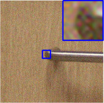
IRCNN (26.98dB)

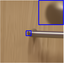
DPIR (35.39dB)

DPIR+ (31.52dB)

CurvPnP (37.30dB)

Figure 12: Single image super-resolution results of different methods on two representative images selected from PolyU dataset.

Single image super-resolution (SISR) aims to improve the resolution and quality of the low-resolution images, which can be described as follows

$$y=(Ax)\downarrow_{s}+n,$$ (17)

where $A$ denotes the blur kernel and $\downarrow_{s}$ denotes downsampling by a factor of $s$, i.e., selecting the upper-left pixel for each distinct $s\times s$ patch.

According to Zhao et al (2016), we solve the $x$ subproblem w.r.t. the single image super-resolution problem by the FFT as follows

$$\scriptsize x_{k+1}\!\!=\!\!\mathcal{F}^{-1}\Big{(}\frac{1}{\alpha_{k}}\big{(}d-\overline{\mathcal{F}(A)}\odot_{s}\frac{(\mathcal{F}(A)d)\Downarrow_{s}}{(\overline{\mathcal{F}(A)}\mathcal{F}(A))\Downarrow_{s}+\alpha_{k}\mathcal{I}}\big{)}\Big{)},$$

where

$$d=\overline{\mathcal{F}(A)}\mathcal{F}(y\uparrow_{s})+\alpha_{k}\mathcal{F}(v_{k}),$$

and $\alpha_{k}=\frac{\lambda\sigma_{s}^{2}}{\sigma_{k}^{2}}$, $\odot_{s}$ denotes element-wise multiplication to the $s\times s$ distinct blocks of $\overline{\mathcal{F}(A)}$, and $\Downarrow_{s}$ denotes averaging the $s\times s$ distinct blocks. Note that the periodic boundary condition is used to guarantee the implementation of FFT.

5.5.1 Comparison methods

Except for aforementioned PnP methods, our CurvPnP is also compared with the representative SISR methods including both model-based method and learning-based method, the details of which are described as follows

• TFOV (Yao et al, 2020): The Total Fractional-Order Variation (TFOV) is the fractional-order TV regularization SISR method, which is solved by the scalar auxiliary variable algorithm.

• ZSSR (Shocher et al, 2018): The Zero-Shot Super-Resolution (ZSSR) is an unsupervised CNN-based zero-shot SR method, which does not require the training samples and prior training.

• SRFBN (Li et al, 2019): The Super-Resolution FeedBack Network (SRFBN) is a recurrent neural network with the feedback mechanism, which was trained on DIV2K and Flickr2K datasets degraded by the bicubic downsampling.

Table 7: Average runtime comparison (in seconds) among different methods on single image super-resolution datasets.

Datasets	TFOV	ZSSR	SRFBN	IRCNN	DPIR	DPIR+	CurvPnP
CC	53.6637	28.5531	0.0914	0.2859	1.2214	0.7311	1.0747
PolyU	52.9980	26.0500	0.0906	0.2854	1.2114	0.6817	1.4411

Table 8: Ablation study on individual components of the proposed C-UNet on CC dataset and CurvPnP on the image “Woman” with the first kernel. The best scores are highlighted.

Task	Mehod	Noise Level Map	Curvature Map	$\sigma_{s}=20$	$\sigma_{s}=35$	$\sigma_{s}=50$
Denoising	UNet	$\times$	$\times$	36.90	36.99	35.26
		$\checkmark$	$\times$	39.64	37.04	35.33
		$\times$	$\checkmark$	39.65	37.05	35.34
		$\checkmark$	$\checkmark$	39.70	37.11	35.40
Task	Mehod	Noise Level Map	Curvature Map	$\sigma_{s}=4$	$\sigma_{s}=6$	$\sigma_{s}=8$
Deblurring	PnP	$\times$	$\times$	27.53	25.82	24.57
		$\checkmark$	$\times$	28.07	26.41	25.23
		$\times$	$\checkmark$	27.71	26.05	24.87
		$\checkmark$	$\checkmark$	28.28	26.69	25.53

5.5.2 Quantitative and qualitative comparison

To test and verify the performance of our CurvPnP, we apply both the degradation of the Gaussian blur kernel with standard deviation 0.7 and the bicubic degradation to the testing images. Since the bicubic downsampling can be approximated by setting a proper blur kernel (Zhang et al, 2020a), the solution of the $x$-sub minimization problem can also be used to solve the bicubic degradation problem. Simultaneously, we consider different combinations of the downsampling factors and noise levels. For the Gaussian blur degradation, we choose the scale factor to be 2 and the noise level of 8 and 16. For the bicubic degradation, both the scale factor 3 with noise level of 4 and the scale factor 4 with noise level of 8 are used for evaluation.

The PSNR of the comparison methods on the RGB channels and Y channel (in YCbCr color space) for CC and PolyU datasets are listed in Table 6. As can be seen, our proposal outperforms the state-of-the-art SISR methods w.r.t. the scale factors and noise levels. In particular, when the scale factor is set as 4 for bicubic degradation, our CurvPnP gains the 0.93dB$\sim$1.67dB higher PSNR on RGB channels and 1.3dB$\sim$1.68dB PSNR on Y channel over DPIR. Simultaneously, our CurvPnP achieves much higher PSNR than DPIR+, which demonstrates the effectiveness of the proposed denoiser. Our CurvPnP can automatically estimate the noise level and remove different noises without knowing the exact noise level and using other noise estimation methods.

Fig. 12 shows the visual comparison results of different methods on the images “NikonD800_4-5_160_1800_classroom_9” from PolyU dataset degraded by the Gaussian blur kernel with the scale factor 2 and $\sigma_{s}=8$, and the image “Canon600D_3-5_125_1600_waterhouse_10” from PolyU dataset corrupted by the bicubic degradation with the scale factor 4 and $\sigma_{s}=8$. In addition to quantitative comparison, our CurvPnP can obtain much vivid images with fine textures and sharp edges as exhibited. As shown in the magnified portions, both DPIR and DPIR+ cannot restore details, while TFOV, ZSSR, SRFBN and IRCNN cannot eliminate noise, but also produce color artifacts. Obviously, our CurvPnP gives the fine structures of the stripes on the chair and the door railing.

5.5.3 Computational efficiency

Table 7 reports the average running time of different methods on the SISR problem with the scale factor 4 and $\sigma_{s}=8$. Since our CurvPnP is terminated by the PSNR values rather than the iteration number, it consumes similar computational time as the DPIR, which is terminated by the fixed iteration numbers of 24 for achieving satisfied restoration results. Although SRFBN, IRCNN and DPIR+ are faster than CurvPnP, their PSNR values are much lower than CurvPnP. The TFOV and ZSSR perform worse than our CurvPnP in terms of restoration performance and running time. Obviously, our CurvPnP achieves the best balance in reconstruction effect and computational efficiency.

5.6 Ablation Studies

The ablation studies are conducted on both image denoising and deblurring problems, where the CC dataset and image “Woman” are used as examples. Our network models are trained on image patches of size 128$\times$128 using a batch size of 16. The numbers of channels are set as 32, 64, 128 and 256 for the first scale to the fourth scale, respectively. Table 8 demonstrates the effectiveness of the noise level map and curvature map by removing them from our model. As shown, taking out the noise level map or curvature map results in the degradation of the restoration. To be specific, PSNR decreases by 0.56dB$\sim$0.66dB and 0.21dB$\sim$0.30dB when noise level map or curvature map are removed for image deblurring. If both noise level map and curvature map modules are removed from the C-UNet, the performance significant drops by 0.75dB$\sim$0.96dB, which demonstrates the advantages of the two modules in investigating and integrating the features.

6 Conclusion

In this paper, we have proposed a novel PnP blind image restoration method, which can be used to effectively deal with various image restoration problems such as image deblurring and super-resolution. More specifically, a new image restoration model was built up by regarding the noise level as a variable. The resulting model was then solved by the penalty method and alternating direction method, where the subproblem w.r.t. the data fidelity was solved by the closed-form solution and both noise level and denoised image were handled by the CNN models. Furthermore, we introduced the ConvNeXt block and curvature supervised attention module into the UNet architecture to enhance the useful features. Numerical results have demonstrated that our CurvPnP outperforms the state-of-the-art PnP methods on different image restoration problems. Compared to the end-to-end learning-based methods, our CurvPnP is more flexible to adapt with different image restoration tasks. Our future work includes to investigate the performance of our CurvPnP on other image restoration problems and to explore effective unsupervised image restoration methods.

References

- \bibcommenthead
- Agustsson and Timofte (2017) Agustsson E, Timofte R (2017) Ntire 2017 challenge on single image super-resolution: Dataset and study. In: Proceedings of the IEEE Conference on Computer Vision and Pattern Recognition Workshops, pp 1122–1131, 10.1109/CVPRW.2017.150
- Bian et al (2021) Bian W, Chen Y, Ye X, et al (2021) An optimization-based meta-learning model for MRI reconstruction with diverse dataset. Journal of Imaging 7(11):231. 10.3390/jimaging7110231
- Bigdeli et al (2020) Bigdeli S, Honzátko D, Süsstrunk S, et al (2020) Image restoration using plug-and-play CNN MAP denoisers. In: VISAPP: Proceedings Of the 15th International Joint Conference on Computer Vision, Imaging and Computer Graphics Theory and Applications, CONF, pp 85–92, 10.5220/0008990700850092
- Boyd et al (2011) Boyd S, Parikh N, Chu E, et al (2011) Distributed optimization and statistical learning via the alternating direction method of multipliers. Foundations and Trends in Machine Learning 3(1):1–122. 10.1561/2200000016
- Brito-Loeza et al (2016) Brito-Loeza C, Chen K, Uc-Cetina V (2016) Image denoising using the Gaussian curvature of the image surface. Numerical Methods for Partial Differential Equations 32(3):1066–1089. 10.1002/num.22042
- Buades et al (2005) Buades A, Coll B, Morel JM (2005) A non-local algorithm for image denoising. In: 2005 IEEE Computer Society Conference on Computer Vision and Pattern Recognition, pp 60–65, 10.1109/CVPR.2005.38
- Chambolle and Pock (2019) Chambolle A, Pock T (2019) Total roto-translational variation. Numerische Mathematik 142(3):611–666. 10.1007/s00211-019-01026-w
- Chan et al (2016) Chan SH, Wang X, Elgendy OA (2016) Plug-and-play ADMM for image restoration: Fixed-point convergence and applications. IEEE Transactions on Computational Imaging 3(1):84–98. 10.1109/TCI.2016.2629286
- Chen et al (2017) Chen D, Mirebeau JM, Cohen LD (2017) Global minimum for a Finsler elastica minimal path approach. International Journal of Computer Vision 122(3):458–483. 10.1007/s11263-016-0975-5
- Chen et al (2015) Chen G, Zhu F, Ann Heng P (2015) An efficient statistical method for image noise level estimation. In: Proceedings of the IEEE International Conference on Computer Vision, pp 477–485, 10.1109/ICCV.2015.62
- Chen et al (2022) Chen M, Quan Y, Pang T, et al (2022) Nonblind image deconvolution via leveraging model uncertainty in an untrained deep neural network. International Journal of Computer Vision 130:1770 C1789. 10.1007/s11263-022-01621-9
- Dabov et al (2007) Dabov K, Foi A, Katkovnik V, et al (2007) Image denoising by sparse 3-D transform-domain collaborative filtering. IEEE Transactions on Image Processing 16(8):2080–2095. 10.1109/TIP.2007.901238
- Dar et al (2016) Dar Y, Bruckstein AM, Elad M, et al (2016) Postprocessing of compressed images via sequential denoising. IEEE Transactions on Image Processing 25(7):3044–3058. 10.1109/TIP.2016.2558825
- Dong et al (2020) Dong J, Roth S, Schiele B (2020) Deep Wiener deconvolution: Wiener meets deep learning for image deblurring. Advances in Neural Information Processing Systems 33:1048–1059. https://proceedings.neurips.cc/paper/2020/hash/0b8aff0438617c055eb55f0ba5d226fa-Abstract.html
- Dong et al (2019) Dong W, Wang P, Yin W, et al (2019) Denoising prior driven deep neural network for image restoration. IEEE Transactions on Pattern Analysis and Machine Intelligence 41(10):2305–2318. 10.1109/TPAMI.2018.2873610
- Dong et al (2011) Dong Y, Hintermüller M, Rincon-Camacho MM (2011) A multi-scale vectorial Lτ-TV framework for color image restoration. International Journal of Computer Vision 92(3):296–307. 10.1007/s11263-010-0359-1
- Franzen (1999) Franzen R (1999) Kodak lossless true color image suite. source: http://r0k us/graphics/kodak 4(2)
- Geman and Yang (1995) Geman D, Yang C (1995) Nonlinear image recovery with half-quadratic regularization. IEEE Transactions on Image Processing 4(7):932–946. 10.1109/83.392335
- Goldluecke and Cremers (2011) Goldluecke B, Cremers D (2011) Introducing total curvature for image processing. In: 2011 International Conference on Computer Vision, pp 1267–1274, 10.1109/ICCV.2011.6126378
- Gong and Sbalzarini (2017) Gong Y, Sbalzarini IF (2017) Curvature filters efficiently reduce certain variational energies. IEEE Transactions on Image Processing 26(4):1786–1798. 10.1109/TIP.2017.2658954
- Gorelick et al (2016) Gorelick L, Veksler O, Boykov Y, et al (2016) Convexity shape prior for binary segmentation. IEEE Transactions on Pattern Analysis and Machine Intelligence 39(2):258–271. 10.1109/TPAMI.2016.2547399
- Gu et al (2020) Gu J, Cai H, Chen H, et al (2020) PIPAL: a large-scale image quality assessment dataset for perceptual image restoration. In: European Conference on Computer Vision, pp 633–651, 10.1007/978-3-030-58621-8_37
- Gu et al (2014) Gu S, Zhang L, Zuo W, et al (2014) Weighted nuclear norm minimization with application to image denoising. In: Proceedings of the IEEE Conference on Computer Vision and Pattern Recognition, pp 2862–2869, 10.1109/CVPR.2014.366
- Gu et al (2018) Gu S, Timofte R, Van Gool L (2018) Integrating local and non-local denoiser priors for image restoration. In: 2018 24th International Conference on Pattern Recognition (ICPR), pp 2923–2928, 10.1109/ICPR.2018.8545043
- Guo et al (2019) Guo S, Yan Z, Zhang K, et al (2019) Toward convolutional blind denoising of real photographs. In: Proceedings of the IEEE/CVF Conference on Computer Vision and Pattern Recognition, pp 1712–1722, 10.1109/CVPR.2019.00181
- He et al (2019) He J, Yang Y, Wang Y, et al (2019) Optimizing a parameterized plug-and-play ADMM for iterative low-dose CT reconstruction. IEEE Transactions on Medical Imaging 38(2):371–382. 10.1109/TMI.2018.2865202
- He et al (2020) He Y, Kang SH, Liu H (2020) Curvature regularized surface reconstruction from point clouds. SIAM Journal on Imaging Sciences 13(4):1834–1859. 10.1137/20M1314525
- Huang et al (2015) Huang JB, Singh A, Ahuja N (2015) Single image super-resolution from transformed self-exemplars. In: Proceedings of the IEEE Conference on Computer Vision and Pattern Recognition, pp 5197–5206, 10.1109/CVPR.2015.7299156
- Kamilov et al (2017) Kamilov US, Mansour H, Wohlberg B (2017) A plug-and-play priors approach for solving nonlinear imaging inverse problems. IEEE Signal Processing Letters 24(12):1872–1876. 10.1109/LSP.2017.2763583
- Levin et al (2009) Levin A, Weiss Y, Durand F, et al (2009) Understanding and evaluating blind deconvolution algorithms. In: IEEE Conference on Computer Vision and Pattern Recognition, pp 1964–1971, 10.1109/CVPR.2009.5206815
- Li and Wu (2019) Li Z, Wu J (2019) Learning deep CNN denoiser priors for depth image inpainting. Applied Sciences 9(6):1103. 10.3390/app9061103
- Li et al (2019) Li Z, Yang J, Liu Z, et al (2019) Feedback network for image super-resolution. In: Proceedings of the IEEE/CVF Conference on Computer Vision and Pattern Recognition, pp 3867–3876, 10.1109/CVPR.2019.00399
- Lim et al (2017) Lim B, Son S, Kim H, et al (2017) Enhanced deep residual networks for single image super-resolution. In: Proceedings of the IEEE Conference on Computer Vision and Pattern Recognition Workshops, pp 136–144, 10.1109/CVPRW.2017.151
- Liu et al (2022a) Liu H, Tai XC, Glowinski R (2022a) An operator-splitting method for the Gaussian curvature regularization model with applications to surface smoothing and imaging. SIAM Journal on Scientific Computing 44(2):A935–A963. 10.1137/21M143772X
- Liu et al (2022b) Liu Z, Mao H, Wu CY, et al (2022b) A convnet for the 2020s. In: Proceedings of the IEEE/CVF Conference on Computer Vision and Pattern Recognition, pp 11,976–11,986, 10.1109/CVPR52688.2022.01167
- Ma et al (2017) Ma K, Duanmu Z, Wu Q, et al (2017) Waterloo exploration database: New challenges for image quality assessment models. IEEE Transactions on Image Processing 26(99):1004–1016. 10.1109/TIP.2016.2631888
- Meinhardt et al (2017) Meinhardt T, Moller M, Hazirbas C, et al (2017) Learning proximal operators: Using denoising networks for regularizing inverse imaging problems. In: Proceedings of the IEEE International Conference on Computer Vision, pp 1781–1790, 10.1109/ICCV.2017.198
- Nam et al (2016) Nam S, Hwang Y, Matsushita Y, et al (2016) A holistic approach to cross-channel image noise modeling and its application to image denoising. In: Proceedings of the IEEE Conference on Computer Vision and Pattern Recognition, pp 1683–1691, 10.1109/CVPR.2016.186
- Ono (2017) Ono S (2017) Primal-dual plug-and-play image restoration. IEEE Signal Processing Letters 24(8):1108–1112. 10.1109/LSP.2017.2710233
- Rond et al (2016) Rond A, Giryes R, Elad M (2016) Poisson inverse problems by the plug-and-play scheme. Journal of Visual Communication and Image Representation 41:96–108. 10.1016/j.jvcir.2016.09.009
- Ryu et al (2019) Ryu E, Liu J, Wang S, et al (2019) Plug-and-play methods provably converge with properly trained denoisers. In: Proceedings of the 36th International Conference on Machine Learning, PMLR, pp 5546–5557, https://proceedings.mlr.press/v97/ryu19a.html
- Schoenemann et al (2012) Schoenemann T, Kahl F, Masnou S, et al (2012) A linear framework for region-based image segmentation and inpainting involving curvature penalization. International Journal of Computer Vision 99:53–68. 10.1007/s11263-012-0518-7
- Shi and Feng (2018) Shi M, Feng L (2018) Plug-and-play prior based on gaussian mixture model learning for image restoration in sensor network. IEEE Access 6:78,113–78,122. 10.1109/ACCESS.2018.2884795
- Shocher et al (2018) Shocher A, Cohen N, Irani M (2018) Zero-shot super-resolution using deep internal learning. In: Proceedings of the IEEE Conference on Computer Vision and Pattern Recognition, pp 3118–3126, 10.1109/CVPR.2018.00329
- Sreehari et al (2016) Sreehari S, Venkatakrishnan SV, Wohlberg B, et al (2016) Plug-and-play priors for bright field electron tomography and sparse interpolation. IEEE Transactions on Computational Imaging 2(4):408–423. 10.1109/TCI.2016.2599778
- Sun et al (2020) Sun Y, Liu J, Kamilov US (2020) Block coordinate regularization by denoising. IEEE Transactions on Computational Imaging 6:908–921. 10.1109/TCI.2020.2996385
- Teodoro et al (2019) Teodoro AM, Bioucas-Dias JM, Figueiredo MA (2019) Image restoration and reconstruction using targeted plug-and-play priors. IEEE Transactions on Computational Imaging 5(4):675–686. 10.1109/TCI.2019.2914773
- Tirer and Giryes (2018) Tirer T, Giryes R (2018) Image restoration by iterative denoising and backward projections. IEEE Transactions on Image Processing 28(3):1220–1234. 10.1109/TIP.2018.2875569
- Tirer and Giryes (2019) Tirer T, Giryes R (2019) Super-resolution via image-adapted denoising CNNs: Incorporating external and internal learning. IEEE Signal Processing Letters 26(7):1080–1084. 10.1109/LSP.2019.2920250
- Ulen et al (2015) Ulen J, Strandmark P, Kahl F (2015) Shortest paths with higher-order regularization. IEEE Transactions on Pattern Analysis and Machine Intelligence 37(12):2588–2600. 10.1109/TPAMI.2015.2409869
- Ulyanov et al (2018) Ulyanov D, Vedaldi A, Lempitsky V (2018) Deep image prior. In: Proceedings of the IEEE Conference on Computer Vision and Pattern Recognition, p 9446 C9454, 10.1109/CVPR.2018.00984
- Unni et al (2018) Unni V, Ghosh S, Chaudhury KN (2018) Linearized ADMM and fast nonlocal denoising for efficient plug-and-play restoration. In: 2018 IEEE Global Conference on Signal and Information Processing (GlobalSIP), pp 11–15, 10.1109/GlobalSIP.2018.8646599
- Venkatakrishnan et al (2013) Venkatakrishnan SV, Bouman CA, Wohlberg B (2013) Plug-and-play priors for model based reconstruction. In: 2013 IEEE Global Conference on Signal and Information Processing, pp 945–948, 10.1109/GlobalSIP.2013.6737048
- Wang et al (2022) Wang C, Zhang Z, Guo Z, et al (2022) Efficient SAV algorithms for curvature minimization problems. IEEE Transactions on Circuits and Systems for Video Technology 10.1109/TCSVT.2022.3217586
- Wei et al (2020) Wei K, Aviles-Rivero A, Liang J, et al (2020) Tuning-free plug-and-play proximal algorithm for inverse imaging problems. In: Proceedings of the 37th International Conference on Machine Learning, PMLR, pp 10,158–10,169, https://proceedings.mlr.press/v119/wei20b.html
- Wei et al (2022) Wei K, Aviles-Rivero A, Liang J, et al (2022) TFPnP: Tuning-free plug-and-play proximal algorithms with applications to inverse imaging problems. Journal of Machine Learning Research 23(16):1–48. http://jmlr.org/papers/v23/20-1297.html
- Xu et al (2018) Xu J, Li H, Liang Z, et al (2018) Real-world noisy image denoising: A new benchmark. arXiv preprint arXiv.1804.02603
- Yair and Michaeli (2018) Yair N, Michaeli T (2018) Multi-scale weighted nuclear norm image restoration. In: Proceedings of the IEEE Conference on Computer Vision and Pattern Recognition, pp 3165–3174, 10.1109/CVPR.2018.00334
- Yao et al (2020) Yao W, Shen J, Guo Z, et al (2020) A total fractional-order variation model for image super-resolution and its SAV algorithm. Journal of Scientific Computing 82(3):1–18. 10.1007/s10915-020-01185-1
- Zamir et al (2021) Zamir SW, Arora A, Khan S, et al (2021) Multi-stage progressive image restoration. In: Proceedings of the IEEE/CVF Conference on Computer Vision and Pattern Recognition, pp 14,816–14,826, 10.1109/CVPR46437.2021.01458
- Zhang et al (2019a) Zhang H, Dai Y, Li H, et al (2019a) Deep stacked hierarchical multi-patch network for image deblurring. In: Proceedings of the IEEE/CVF Conference on Computer Vision and Pattern Recognition, pp 5971–5979, 10.1109/CVPR.2019.00613
- Zhang et al (2017a) Zhang J, Pan J, Lai WS, et al (2017a) Learning fully convolutional networks for iterative non-blind deconvolution. In: Proceedings of the IEEE Conference on Computer Vision and Pattern Recognition, pp 3817–3825, 10.1109/CVPR.2017.737
- Zhang and Timofte (2022) Zhang K, Timofte R (2022) Deep plug-and-play and deep unfolding methods for image restoration. In: Advanced Methods and Deep Learning in Computer Vision. Elsevier, p 481–509, 10.1016/B978-0-12-822109-9.00023-0
- Zhang et al (2017b) Zhang K, Zuo W, Chen Y, et al (2017b) Beyond a Gaussian denoiser: Residual learning of deep CNN for image denoising. IEEE Transactions on Image Processing 26(7):3142–3155. 10.1109/TIP.2017.2662206
- Zhang et al (2017c) Zhang K, Zuo W, Gu S, et al (2017c) Learning deep CNN denoiser prior for image restoration. In: Proceedings of the IEEE Conference on Computer Vision and Pattern Recognition, pp 3929–3938, 10.1109/CVPR.2017.300
- Zhang et al (2018) Zhang K, Zuo W, Zhang L (2018) FFDNet: Toward a fast and flexible solution for CNN-based image denoising. IEEE Transactions on Image Processing 27(9):4608–4622. 10.1109/TIP.2018.2839891
- Zhang et al (2019b) Zhang K, Zuo W, Zhang L (2019b) Deep plug-and-play super-resolution for arbitrary blur kernels. In: Proceedings of the IEEE/CVF Conference on Computer Vision and Pattern Recognition, pp 1671–1681, 10.1109/CVPR.2019.00177
- Zhang et al (2020a) Zhang K, Van Gool L, Timofte R (2020a) Deep unfolding network for image super-resolution. In: Proceedings of the IEEE/CVF Conference on Computer Vision and Pattern Recognition, pp 3217–3226, 10.1109/CVPR42600.2020.00328
- Zhang et al (2022) Zhang K, Li Y, Zuo W, et al (2022) Plug-and-play image restoration with deep denoiser prior. IEEE Transactions on Pattern Analysis and Machine Intelligence 44(10):6360–6376. 10.1109/TPAMI.2021.3088914
- Zhang et al (2020b) Zhang X, Dong H, Hu Z, et al (2020b) Gated fusion network for degraded image super resolution. International Journal of Computer Vision 128(6):1699–1721. 10.1007/s11263-019-01285-y
- Zhao et al (2016) Zhao N, Wei Q, Basarab A, et al (2016) Fast single image super-resolution using a new analytical solution for C problems. IEEE Transactions on Image Processing 25(8):3683–3697. 10.1109/TIP.2016.2567075
- Zhao and Liang (2020) Zhao S, Liang H (2020) Multi-frame super resolution via deep plug-and-play CNN regularization. Journal of Inverse and Ill-posed Problems 28(4):533–555. 10.1515/jiip-2019-0054
- Zheng et al (2021) Zheng D, Tan SH, Zhang X, et al (2021) An unsupervised deep learning approach for real-world image denoising. In: International Conference on Learning Representations, https://openreview.net/forum?id=tIjRAiFmU3y
- Zhong et al (2020) Zhong Q, Li Y, Yang Y, et al (2020) Minimizing discrete total curvature for image processing. In: Proceedings of the IEEE/CVF Conference on Computer Vision and Pattern Recognition, pp 9474–9482, 10.1109/CVPR42600.2020.00949
- Zhong et al (2021) Zhong Q, Yin K, Duan Y (2021) Image reconstruction by minimizing curvatures on image surface. Journal Mathematical Imaging and Vision 63(1):30–55. 10.1007/s10851-020-00992-3
- Zhong et al (2022) Zhong Q, Liu RW, Duan Y (2022) Spatially adapted first and second order regularization for image reconstruction: From an image surface perspective. Journal of Scientific Computing 92(2):33. 10.1007/s10915-022-01886-9
- Zoran and Weiss (2011) Zoran D, Weiss Y (2011) From learning models of natural image patches to whole image restoration. In: 2011 International Conference on Computer Vision, pp 479–486, 10.1109/ICCV.2011.6126278