SNIPER TRAINING: VARIABLE SPARSITY RATE TRAINING FOR TEXT-TO-SPEECH

Abstract

Text-to-speech (TTS) models have achieved remarkable naturalness in recent years, yet like most deep neural models, they have more parameters than necessary. Sparse TTS models can improve on dense models via pruning and extra retraining, or converge faster than dense models with some performance loss. Inspired by these results, we propose training TTS models using a decaying sparsity rate, i.e. a high initial sparsity to accelerate training first, followed by a progressive rate reduction to obtain better eventual performance. This decremental approach differs from current methods of incrementing sparsity to a desired target, which costs significantly more time than dense training. We call our method SNIPER training: Single-shot Initialization Pruning Evolving-Rate training. Our experiments on FastSpeech2 show that although we were only able to obtain better losses in the first few epochs before being overtaken by the baseline, the final SNIPER-trained models beat constant-sparsity models and pip dense models in performance.

Index Terms—  speech synthesis, text-to-speech, sparsity, network pruning, training acceleration

1 Introduction

Although classical learning requires $n$ parameters to fit $n$ data points, [1] showed that large over-parameterized models with at least $nd$ parameters are in fact necessary for smooth interpolation (where $d$ is the data dimensionality). This explains the recent trend towards ever-larger neural models, but we have now reached the era of extreme diminishing returns – [2] found that the compute power needed to reduce error rates by a factor of $x$ was at least $x^{10}$ across a range of image classification and natural language processing tasks.

Counteracting this, researchers have proposed methods to compress models, ranging from tensor decomposition and quantization to parameter sharing. The most flexible approaches involve sparsification techniques, which can be applied at different stages of training and network architectures. [3] comprehensively surveyed sparse approaches, dividing their utility into (1) improved generalization and (2) reducing memory requirements. For (1), sparse approaches have been shown to reduce overfitting and boost robustness [4]; an especially ubiquitous technique is Dropout [5], which uses ephemeral sparsity. For (2), dominant techniques look at how to achieve similar performance or better with a subset of the original parameters; the Lottery Ticket Hypothesis [6] proposes that when a dense network is initialized, some subnetworks (winning tickets) can match the same-iteration performance of the full network when trained in isolation.

[6] provides evidence for the hypothesis by employing iterative magnitude pruning, which repeatedly trains dense networks and prunes the lowest-magnitude weights to obtain a binary mask $m$. After applying the obtained masks to the weights at initialization, the sparse model can converge faster and obtain better accuracy than the dense one. This technique mirrors the adolescent brain, which grows neurons and prunes connections as it learns, and has been demonstrated in brain simulations [7].

More recent analysis [8], however, suggests the winning tickets cannot be found without prior dense training and therefore requires much more time to train than the original unpruned model. The additional time taken holds (to a smaller extent) for other sparsification schemes like dynamic pruning, which regrows weights during training according to gradients [9] or momentum [10] in each backward pass. Moreover, barring very high sparsities (above 80% for 2-D float32 tensors), sparse models offer no improvement in memory usage or training and inference time.

Since the goal is not just to produce a sparse model, we propose a sparse training scheme that progressively decreases sparsity to 0 rather than increases it to a target sparsity. Intuitively, we want to direct gradient updates to more important weights at the start for faster convergence and let the less important ones update later. We apply our method on FastSpeech2 [11] and evaluate its effectiveness via naturalness, intelligibility, prosody, and training time, comparing it to both dense and constant-sparsity models. We observe that the final SNIPER-trained models surpass the constant-sparsity models on nearly all the metrics and edges out the dense model in most. Finally, we discuss how to optimize such a sparse training scheme, as we believe new easy-to-apply techniques that speed up training and/or improve performance have been lacking for deep learning tasks and especially TTS.

In the next section, we introduce fast sparse training, followed by SNIPER training in Section 3, our experiment setup in Section 4, results in Section 5 and discussion in Section 6.

2 Related Work on Fast Sparse Training

2.1 Hardware-Dependent Training

There is a large body of research that proposes neural net accelerators on the hardware level [12]. Generally, these schemes [13] take advantage of sparsity to reorder computations such that operations resulting in zero are skipped [14]; convolutions are especially amenable to such pruning [15].

Such hardware designs, however, have not been commercially realized. The closest available currently is the NVIDIA A100 GPU, where speed doubles if 2:4 sparsity is satisfied in a tensor (i.e. every block of 4 elements has 2 zeros). [16] was the first to exploit this: they pruned the smallest weights from $\mathcal{W}$ to $\widetilde{\mathcal{W}}$ in each block before the forward pass. After the backward pass, they corrected the approximation error by changing the familiar update $\mathcal{W}_{t+1}=\mathcal{W}_{t}-\alpha_{t}g(\widetilde{\mathcal{W}}_{t})$ to $\mathcal{W}_{t+1}=\mathcal{W}_{t}-\alpha_{t}(g(\widetilde{\mathcal{W}}_{t})+\lambda(m_{t}\odot\mathcal{W}_{t}))$ where $\alpha$ is the learning rate, $g$ is the gradient, $\lambda$ is a relative weight and $m$ is the weights mask. To allow sparse speedup on the backward pass as well, [17] proposed a greedy pruning method to find transposable masks that had the 2:4 property both row-wise and column-wise. They further proved that their method ensured the $\ell_{1}$-norm of the pruned weights $W(P)$ was at most $<2W^{*}$ (weights from optimal pruning).

2.2 Increasing Model Size

Aside from hardware-specific methods, another approach to sparse speedups is ironically to explode parameter count. This was done in the 1.6 trillion parameter Switch-Transformer model [18], which trained up to 4$\times$ faster than T5-XXL [19]. While the original Transformer model contains a single dense feed-forward layer after each multi-head attention layer, the Switch-Transformer replaces it with many (2,048) feed-forward blocks with a routing mechanism that decides which block should receive the attention output – a variant of the Mixture-of-Experts technique, where each block is an expert. In this way, the feed-forward blocks are sparse (most are not used during training or inference), while training is accelerated as the data and feed-forward blocks can be parallelized.

Dee to these shortcomings, there is still a largely unexplored space of hardware-independent sparse techniques that can accelerate training and maintain model size, which we attempt to address.

3 SNIPER Training for TTS

3.1 Sparsity in TTS

Studies investigating sparsity in TTS are rare due to a few factors. TTS is generative in nature and harder to evaluate automatically, leading to ambiguity in proving technique effectiveness. Also, complex architectures impede component-wise characterization of sparse behaviour.

Initial work in this direction [20] showed that both text-to-mel and vocoder models could be pruned, while output quality could be maintained or even improved. This was achieved by pruning the models (with zero weights allowed to be updated), training to convergence, and re-pruning. [21] further tested five sparse techniques on a Tacotron2 baseline and demonstrated comparable performance when pruning before, during, or after training. Remarkably, using single-shot network initialization pruning (SNIP) allowed the model to reach minimum loss at least 1.9$\times$ faster at 40% sparsity, although quality degraded slightly.

3.2 SNIP

SNIP [22] is one among many foresight pruning methods that obtain a pruning mask before training begins. It ranks the importance of a neural network weight by the estimated change in loss when it is set to zero. That is, for a binary mask $\bm{m}$, the effect of removing connection $j$ on the loss $\mathcal{L}_{j}$ is

$$\Delta\mathcal{L}_{j}(\bm{\mathrm{w}};\mathcal{D})\approx g_{j}(\bm{\mathrm{w}};\mathcal{D})=\left.\frac{\partial\mathcal{L}(\bm{m}\odot\bm{\mathrm{w}};\mathcal{D})}{\partial m_{j}}\right|_{\bm{m=1}}$$

Other prominent foresight pruning methods include (1) Gradient Signal Preservation [23], a second-order extension of SNIP which calculates the gradient Hessian to compensate for correlated weights; (2) Neural Tangent Transfer, [24], a label-free approach which finds a sparse network linearly approximating the training evolution of the dense network; and (3) SynFlow [25], a data-free approach that avoids layer collapse by iteratively pruning the weights with the lowest $\ell_{1}$-path norm. Further techniques involve comparing activation function output or weight magnitudes, possibly with lookahead to downstream layers [26]. Nonetheless, [27] compared 13 of these pruning algorithms on image classification and found SNIP to be the most consistent performer over multiple sparsities and also relatively simpler to implement.

3.3 SNIPER Training

We implemented SNIP by saving the initial model weights and masking all specified trainable weights, then computing the gradient with respect to the weights. The gradients were accumulated over the entire training dataset and saved (this takes 1 epoch since we use the whole training corpus). Once the gradients were computed, we generate masks with different sparsities by simply removing the lowest absolute gradients; this takes very little time and the masks are reusable. The various masks can be swapped during training according to a given schedule, which constitutes the evolving-rate part of SNIPER.

We allow multiple options besides specifying the schedule. These include: (1) scaling individual parameter learning rates by $1/(1-sparsity)$, (2) limiting the sparsity of parameters to prevent bottlenecks, (3) limiting the maximum parameter learning rate, (3) excluding parameters by name, (4) restoring newly activated weights during a sparsity reduction either to zeros or the initial model values, (5) using a subset of the training corpus for gradient computation with a batch iterator, and (6) resuming from a previous state. Our SNIPER library is available on Github.

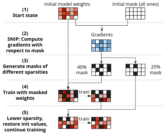
Fig. 1: Example of SNIPER training process with 40% initial sparsity reducing to 20%.

4 Experiments

4.1 Baseline and Dataset

We use the open-source ESPnet2 [28] version of FastSpeech2 with default settings and a pretrained ParallelWaveGAN [29] vocoder. Notably, the Xavier initialization used ensures that variance is consistent throughout the network, which is important for SNIP. The ground-truth durations were generated by Montreal Forced Aligner (MFA) according to the original paper [11]. We train FastSpeech2 for 400 epochs (320k steps) on the LJSpeech [30] dataset with an 80:10:10 train-validation-eval split. In all experiments, the same initial values and random seed were used to reduce variability. All of our experiments and data are available on Github.

4.2 SNIPER

In our experiments, we exclude the embedding and normalization layers and set initial sparsity to 20% and 40% with a maximum individual sparsity of 75% (causing overall model sparsity to be 19.8% and 38.2%). For comparison, we also reduce sparsity to 0% according to the schedules shown in Table 2. We thus compare 5 models in total, which is reported in Table 1. These decisions are justified in the Discussion section.

Table 1: Sparsity settings of compared models.

Baseline	Constant	SNIPER
0%	20%	20 to 0%
	40%	40 to 0%

Table 2: Schedules for 20 to 0% (left) and 40 to 0% (right).

Epoch	Sparsity
1-5	20%
6-10	10%
>10	0%

Epoch	Sparsity
1-5	40%
6-10	20%
11-20	10%
>20	0%

5 Results

5.1 Naturalness

Naturalness was measured via mean opinion score (MOS) [31] from 1 (worst) to 5 (best). 10 randomly-chosen utterances were generated on each setting; 5 by the best model during validation and 5 by the model at the end of training. MOS for the ground truth samples (Natural) is included for reference. SNIPER training marginally gave the most consistent improvements over the baseline, as reported in Table 3.

Table 3: MOS. Average scores across best-validation and end-of-training models. Bold = best model for given sparsity.

Sparsity	Baseline	Constant	SNIPER	Natural
20%	3.774	3.876	3.804	4.454
40%		3.691	3.775

We also did a three-way preference test between the Baseline, Constant and SNIPER samples at 20% and 40% sparsities with 16 utterances each (split by best-validation and end-of-training models). Participants were asked to rate the best and worst samples in each set of 3. As we asked them to rate the same sample for both best and worst if they could not decide, we report % rated best minus % rated worst for each setting. All tests were run on PsyToolkit [32] [33] and we obtained 19 full responses. The SNIPER-trained models were preferred in most settings, as reported in Table 4.

Table 4: Preference test. Bold = best model for given setting.

Sparsity (setting)	Baseline	Constant	SNIPER
20% (best validation)	2.6	-12.0	9.4
40% (best validation)	1.6	-10.4	8.9
20% (end of training)	7.8	1.6	-9.4
40% (end of training)	-4.2	-3.6	7.8

5.2 Intelligibility

We used the commercial Speechmatics engine to transcribe the generated audio across the entire test set for each model, and measured intelligibility by the word error rate (WER) of the transcript against the normalized LJSpeech text. We note that the SNIPER-trained models starting at 20% sparsity perform slightly better than baseline, although differences are minimal (possibly due to LJSpeech being common training data for speech recognition engines).

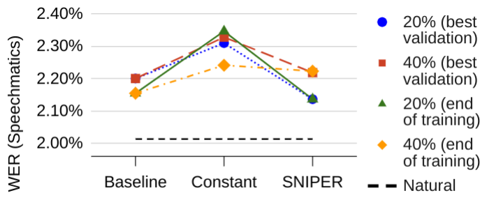
Fig. 2: WER weighted by ground truth length.

5.3 Prosody

Mean F0-RMSE  [34] across the entire test set was used to quantify prosody differences between ground truth recordings and generated audio. Consistent with other findings, the end-of-training 40 to 0% SNIPER model performs slightly better than the other models (Figure 3).

Fig. 3: F0-RMSE (in cents) across all experiment settings.

5.4 Training time

All experiments were run on a single GeForce RTX3090 GPU. Calculating SNIP gradients across the whole dataset took 7.7 minutes and mask creation took less than 1 second (one-time operation). The slight delay in training sparse models comes from masking during the forward pass.

Table 5: Training time in hours.

Sparsity	Baseline	Constant	SNIPER
20%	13.1	13.5	13.1
40%		13.5	13.2

6 Discussion

Our schedules were informed by the training and validation losses of the constant-sparsity runs. We start decreasing sparsity when the loss exceeds the dense model at the same epoch.

Fig. 4: Early loss curves for baseline against constant 40% sparsity (left: training, right: validation). Above 10 epochs, the baseline always gets lower training loss.

We note that our results differ from [21], where the sparse Tacotron2 Double Decoder Consistency model converged faster than the dense one. Investigating the top-5 pruned components in that model shows the coarse decoder ($r=6$) to be the main source of pruned weights at 40% sparsity. This implies that the coarse decoder, which exactly copies the structure of the original $r=1$ decoder, is over-parameterized and should be pruned (expected as its main function is to accelerate attention alignment learning [35]). When we tried SNIPER training on ESPnet’s Tacotron2 version, which has only one decoder, there was no training benefit.

Furthermore, the top-5 pruned parameters (ignoring bias values) in FastSpeech2 at 40% sparsity were all from the postnet. We believe that pruning the postnet does not help, since we retrained FastSpeech2 without the postnet and there was almost no impact on the loss after 20 epochs.

We now explain our chosen hyperparameters, which should guide future option choices in SNIPER training. While searching for a scheme that provides better loss curves than the dense model, we found that, for both training and validation loss,

• Scaling overall learning rate by sparsity is better than no scaling

• Scaling learning rate by parameter beats simply scaling the overall learning rate

• Limiting maximum sparsity offers improvements in the above cases.

Loss plots for the above are posted on our Github page.

7 Conclusion

Our method, SNIPER training, is the first attempt at using sparsity to accelerate TTS training. Though we could not make FastSpeech2 converge faster beyond the initial epochs, we have shown the SNIPER-trained models to be clearly superior to plain sparse models and slightly better than dense models. Moreover, we have analysed how TTS architecture may influence SNIPER effectiveness, and provide suggestions on the ideal settings for others to apply our work. Further development could allow automatic sparsity selection during training based on convergence rate, or improve on dropout, which is a random and less directed form of sparsity.

8 References

References

- [1] S. Bubeck and M. Sellke, “A universal law of robustness via isoperimetry,” in Advances in Neural Information Processing Systems 34, 2021, pp. 28 811–28 822.
- [2] N. C. Thompson, K. H. Greenewald, K. Lee, and G. F. Manso, “The computational limits of deep learning,” CoRR, vol. abs/2007.05558, 2020.
- [3] T. Hoefler, D. Alistarh, T. Ben-Nun, N. Dryden, and A. Peste, “Sparsity in deep learning: Pruning and growth for efficient inference and training in neural networks,” J. Mach. Learn. Res., vol. 22, pp. 241:1–241:124, 2021.
- [4] T. Chen, Z. Zhang, P. Wang, S. Balachandra, H. Ma, Z. Wang, and Z. Wang, “Sparsity winning twice: Better robust generalization from more efficient training,” in The Tenth International Conference on Learning Representations, ICLR, 2022.
- [5] N. Srivastava, G. E. Hinton, A. Krizhevsky, I. Sutskever, and R. Salakhutdinov, “Dropout: a simple way to prevent neural networks from overfitting,” J. Mach. Learn. Res., vol. 15, no. 1, pp. 1929–1958, 2014.
- [6] J. Frankle and M. Carbin, “The lottery ticket hypothesis: Finding sparse, trainable neural networks,” in 7th International Conference on Learning Representations, ICLR, 2019.
- [7] B. B. Averbeck, “Pruning recurrent neural networks replicates adolescent changes in working memory and reinforcement learning,” Proceedings of the National Academy of Sciences, vol. 119, no. 22, p. e2121331119, 2022.
- [8] J. Maene, M. Li, and M. Moens, “Towards understanding iterative magnitude pruning: Why lottery tickets win,” CoRR, vol. abs/2106.06955, 2021.
- [9] X. Dai, H. Yin, and N. K. Jha, “Nest: A neural network synthesis tool based on a grow-and-prune paradigm,” IEEE Transactions on Computers, vol. 68, no. 10, pp. 1487–1497, oct 2019.
- [10] T. Dettmers and L. Zettlemoyer, “Sparse networks from scratch: Faster training without losing performance,” arXiv preprint arXiv:1907.04840, 2019.
- [11] Y. Ren, C. Hu, X. Tan, T. Qin, S. Zhao, Z. Zhao, and T. Liu, “Fastspeech 2: Fast and high-quality end-to-end text to speech,” in 9th International Conference on Learning Representations, ICLR, 2021.
- [12] Y. Chen, Y. Xie, L. Song, F. Chen, and T. Tang, “A survey of accelerator architectures for deep neural networks,” Engineering, vol. 6, no. 3, pp. 264–274, 2020.
- [13] S. Zhang, Z. Du, L. Zhang, H. Lan, S. Liu, L. Li, Q. Guo, T. Chen, and Y. Chen, “Cambricon-x: An accelerator for sparse neural networks,” in 49th Annual IEEE/ACM International Symposium on Microarchitecture (MICRO), 2016, pp. 1–12.
- [14] J. Zhang, X. Chen, M. Song, and T. Li, “Eager pruning: Algorithm and architecture support for fast training of deep neural networks,” in ACM/IEEE 46th Annual International Symposium on Computer Architecture (ISCA), 2019, pp. 292–303.
- [15] M. Soltaniyeh, R. P. Martin, and S. Nagarakatte, “An accelerator for sparse convolutional neural networks leveraging systolic general matrix-matrix multiplication,” ACM Trans. Archit. Code Optim., vol. 19, no. 3, may 2022.
- [16] A. Zhou, Y. Ma, J. Zhu, J. Liu, Z. Zhang, K. Yuan, W. Sun, and H. Li, “Learning N: M fine-grained structured sparse neural networks from scratch,” in 9th International Conference on Learning Representations, ICLR, 2021.
- [17] I. Hubara, B. Chmiel, M. Island, R. Banner, J. Naor, and D. Soudry, “Accelerated sparse neural training: A provable and efficient method to find n: m transposable masks,” Advances in Neural Information Processing Systems, vol. 34, pp. 21 099–21 111, 2021.
- [18] W. Fedus, B. Zoph, and N. Shazeer, “Switch transformers: Scaling to trillion parameter models with simple and efficient sparsity,” Journal of Machine Learning Research, vol. 23, no. 120, pp. 1–39, 2022.
- [19] C. Raffel, N. Shazeer, A. Roberts, K. Lee, S. Narang, M. Matena, Y. Zhou, W. Li, and P. J. Liu, “Exploring the limits of transfer learning with a unified text-to-text transformer,” J. Mach. Learn. Res., vol. 21, pp. 140:1–140:67, 2020.
- [20] C.-I. J. Lai, E. Cooper, Y. Zhang, S. Chang, K. Qian, Y.-L. Liao, Y.-S. Chuang, A. H. Liu, J. Yamagishi, D. Cox, and J. Glass, “On the interplay between sparsity, naturalness, intelligibility, and prosody in speech synthesis,” in IEEE International Conference on Acoustics, Speech and Signal Processing (ICASSP), 2022, pp. 8447–8451.
- [21] P. Lam, H. Zhang, N. F. Chen, and B. Sisman, “EPIC TTS models: Empirical pruning investigations characterizing text-to-speech models,” in 23rd Annual Conference of the International Speech Communication Association, INTERSPEECH. ISCA, 2022, pp. 823–827.
- [22] N. Lee, T. Ajanthan, and P. H. S. Torr, “Snip: single-shot network pruning based on connection sensitivity,” in 7th International Conference on Learning Representations, ICLR, 2019.
- [23] C. Wang, G. Zhang, and R. B. Grosse, “Picking winning tickets before training by preserving gradient flow,” in 8th International Conference on Learning Representations, ICLR, 2020.
- [24] T. Liu and F. Zenke, “Finding trainable sparse networks through neural tangent transfer,” in Proceedings of the 37th International Conference on Machine Learning, ICML, vol. 119. PMLR, 2020, pp. 6336–6347.
- [25] H. Tanaka, D. Kunin, D. L. K. Yamins, and S. Ganguli, “Pruning neural networks without any data by iteratively conserving synaptic flow,” in Advances in Neural Information Processing Systems 33: NeurIPS, 2020.
- [26] J. Lee, S. Park, S. Mo, S. Ahn, and J. Shin, “Layer-adaptive sparsity for the magnitude-based pruning,” in 9th International Conference on Learning Representations, ICLR, 2021.
- [27] N. James, “Gauging the state-of-the-art for foresight weight pruning on neural networks,” Bachelor’s Thesis, University of Arkansas, Fayetteville, 2022.
- [28] T. Hayashi, R. Yamamoto, T. Yoshimura, P. Wu, J. Shi, T. Saeki, Y. Ju, Y. Yasuda, S. Takamichi, and S. Watanabe, “Espnet2-tts: Extending the edge of TTS research,” CoRR, vol. abs/2110.07840, 2021.
- [29] R. Yamamoto, E. Song, and J.-M. Kim, “Parallel wavegan: A fast waveform generation model based on generative adversarial networks with multi-resolution spectrogram,” in IEEE International Conference on Acoustics, Speech and Signal Processing (ICASSP), 2020, pp. 6199–6203.
- [30] K. Ito and L. Johnson, “The lj speech dataset,” https://keithito.com/LJ-Speech-Dataset/, 2017.
- [31] Methods for subjective determination of transmission quality, ITU-T Recommendations Std. P.800, 1996.
- [32] G. Stoet, “Psytoolkit: A software package for programming psychological experiments using linux,” Behavior Research Methods, vol. 42, pp. 1096–1104, 2010.
- [33] ——, “Psytoolkit: A novel web-based method for running online questionnaires and reaction-time experiments,” Teaching of Psychology, vol. 44, no. 1, pp. 24–31, 2017.
- [34] T. Hayashi, A. Tamamori, K. Kobayashi, K. Takeda, and T. Toda, “An investigation of multi-speaker training for wavenet vocoder,” in IEEE Automatic Speech Recognition and Understanding Workshop (ASRU), 2017, pp. 712–718.
- [35] E. Gölge, “Solving attention problems of tts models with double decoder consistency,” https://coqui.ai/blog/tts/solving-attention-problems-of-tts-models-with-double-decoder-consistency/, 2020.