Specification and Verification With the TLA⁺ Trifecta: TLC, Apalache, and TLAPS

Abstract

Using an algorithm due to Safra for distributed termination detection as a running example, we present the main tools for verifying specifications written in TLA⁺. Examining their complementary strengths and weaknesses, we suggest a workflow that supports different types of analysis and that can be adapted to the desired degree of confidence.

1 Introduction

TLA⁺ [13] is a formal language for specifying systems, in particular concurrent and distributed algorithms, at a high level of abstraction. The foundations of TLA⁺ are classical Zermelo-Fraenkel set theory with choice for representing the data structures on which the algorithm operates, and the Temporal Logic of Actions (TLA), a variant of linear-time temporal logic, for describing executions of the algorithm.

Most users write TLA⁺ specifications using one of the two existing IDEs (integrated development environments): the TLA⁺ Toolbox [11], a standalone Eclipse application, and a Visual Studio Code Extension, which can be run in a standard Web browser. To different degrees, both IDEs also integrate the three main tools for verifying TLA⁺ specifications: the explicit-state model checker tlc [16], the symbolic SMT-based model checker apalache [8], and the TLA⁺ Proof System tlaps [2], an interactive proof assistant.

In this paper, we use a non-trivial algorithm for detecting termination of an asychronous distributed system [5] as a running example for presenting the three tools. Based on their complementary strengths and weaknesses, we suggest a workflow that can serve as a guideline for analyzing different kinds of properties of a TLA⁺ specification, to different degrees of confidence. This is the first paper that applies all three tools to a common specification and identifies their complementary qualities. We hope that future TLA⁺ users will find our presentation useful for applying these tools to their own specifications. All of our TLA⁺ modules and ancillary files for running the tools are available online [9].

Outline of the paper.

Section 2 presents a high-level specification of the problem of termination detection written as a TLA⁺ state machine, whose properties are verified in Section 3. Safra’s algorithm is informally presented in Section 4. Section 5 describes different approaches for verifying the properties of the algorithm using model checking and theorem proving, including checking that the algorithm refines the high-level specification introduced earlier. Finally, Section 6 concludes the paper and outlines ideas for future work.

2 Specifying Termination Detection

Before presenting Safra’s algorithm for detecting termination of processes on a ring, we formally state the problem to be solved. Although this is not strictly required for using TLA⁺, it will allow us to succinctly state correctness of the algorithm in terms of refinement, and to introduce the TLA⁺ tools on a small specification.

(a) Visual representation.

•     module AsynchronousTerminationDetection    

  $\mbox{\sc extends}\ \ Naturals$
  $\mbox{\sc constant}\ \ N$
  $\mbox{\sc assume}\ \ NAssumption\ \mathrel{\smash{\stackrel{{\scriptstyle\scriptscriptstyle\Delta}}{{=}}}}\ N\in Nat\setminus\{0\}$
  $Node\ \mathrel{\smash{\stackrel{{\scriptstyle\scriptscriptstyle\Delta}}{{=}}}}\ 0\,..\,N\!-\!1$
  $\mbox{\sc variables}\ \ active,pending,termDetect$
  $TypeOK\ \mathrel{\smash{\stackrel{{\scriptstyle\scriptscriptstyle\Delta}}{{=}}}}\ \begin{array}[t]{@{\mbox{$\land$\ }}l@{}}active\in[Node\rightarrow\mbox{\sc boolean}]\\ pending\in[Node\rightarrow Nat]\\ termDetect\in\mbox{\sc boolean}\end{array}$
  $vars\ \mathrel{\smash{\stackrel{{\scriptstyle\scriptscriptstyle\Delta}}{{=}}}}\ \langle active,pending,termDetect\rangle$
  $terminated\ \mathrel{\smash{\stackrel{{\scriptstyle\scriptscriptstyle\Delta}}{{=}}}}$
     $\forall n\in Node:\lnot active[n]\land pending[n]=0$

      

(b) TLA⁺ representation of the state space.

Figure 1: The ring of nodes and its TLA⁺ representation.

As illustrated in Fig. 1(a), we assume $N$ nodes that perform some distributed computation. Each node can be active (indicated by a double circle) or inactive (single circle). When a node is active, it may perform some local computation, and it can send messages to other nodes. Messages can be understood as carrying tasks to be performed by the receiver: an inactive node can still receive messages and will then become active. The purpose of the algorithm is to detect whether all nodes are inactive. Note that the ring structure indicated in Fig. 1(a) is unimportant for the statement of the problem: it will become relevant for the termination detection algorithm to be introduced later.

Figure 1(b) contains the initial part of a TLA⁺ specification that formally states the problem of termination detection. Specifications appear in TLA⁺ modules that contain declarations of constant and variable parameters, statements of assumptions and theorems, but mainly contain operator definitions of the form $Op(args)\mathrel{\smash{\stackrel{{\scriptstyle\scriptscriptstyle\Delta}}{{=}}}}expr$; if the operator does not take arguments, the empty pair of brackets is omitted.

Whereas constant parameters are interpreted by fixed (state-independent) values, variable parameters correspond to state variables that represent the evolution of a system: a state assigns values to variables. TLA⁺ expressions are classified in four levels: constant formulas do not contain any variables, thus their value is the same at all states during the execution of a system. State formulas may contain constants and unprimed variables, and such formulas are evaluated at individual states. Action formulas may additionally contain primed variables; they are evaluated over pairs $(s,t)$ of states: an unprimed variable $v$ denotes the value of $v$ in $s$ whereas the primed variable $v^{\prime}$ denotes the value of $v$ in $t$. Finally, temporal formulas involve operators of temporal logic such as $\Box$ (always) and $\Diamond$ (eventually), and they are evaluated over (infinite) sequences of states. By abuse of language, we will sometimes say that a module defines a state predicate rather than that it defines an operator representing a Boolean state formula, and similarly for the other levels.

TLA⁺ modules form a hierarchy by extending and instantiating other modules. Module $AsynchronousTerminationDetection$ extends module $Naturals$ from the standard library in order to import the definition of the set $Nat$ of natural numbers and standard arithmetic operations. It declares a constant parameter $N$ and defines the constant $Node$ as the interval of integers between $0$ and $N-1$. It also declares variable parameters $active$, $pending$, and $termDetect$, intended to represent the status of each node (active or inactive), the number of pending messages at each node, and whether termination has been detected or not. TLA⁺ is untyped, but it is good engineering practice to document the expected types of constants and variables using a formula of the shape $v\in S$ where $S$ is a set that denotes the type of $v$. Thus, assumption $NAssumption$ states that $N$ must be a non-zero natural number, and the state predicate $TypeOK$ indicates the expected types of the variables: $active$ and $pending$ are Boolean and natural-number valued functions over $Node$, whereas $termDetect$ is a Boolean value. The formal status of the two typing predicates is quite different: an instance of the module that does not satisfy $NAssumption$ is considered illegal, whereas $TypeOK$ just defines a predicate. (We will later check that the predicate indeed holds at every state during any execution.) Finally, the module declares a predicate $terminated$ that is true at states in which the system has globally terminated: all nodes are inactive, and no message is pending at any node.

• $Init\ \mathrel{\smash{\stackrel{{\scriptstyle\scriptscriptstyle\Delta}}{{=}}}}$

  $\begin{array}[t]{@{\mbox{$\land$\ }}l@{}}active\in[Node\rightarrow\mbox{\sc boolean}]\\ pending=[n\in Node\mapsto 0]\\ termDetect\in\{\textsc{false},terminated\}\end{array}$

  $Terminate(i)\ \mathrel{\smash{\stackrel{{\scriptstyle\scriptscriptstyle\Delta}}{{=}}}}$

  $\begin{array}[t]{@{\mbox{$\land$\ }}l@{}}active[i]\\ active^{\prime}=[active\ \mbox{\sc except}\ ![i]=\textsc{false}]\\ pending^{\prime}=pending\\ termDetect^{\prime}\in\{termDetect,terminated^{\prime}\}\end{array}$

  $SendMsg(i,j)\ \mathrel{\smash{\stackrel{{\scriptstyle\scriptscriptstyle\Delta}}{{=}}}}$

  $\begin{array}[t]{@{\mbox{$\land$\ }}l@{}}active[i]\\ pending^{\prime}=[pending\ \mbox{\sc except}\ ![j]=@+1]\\ \mbox{\sc unchanged}\ \langle active,termDetect\rangle\end{array}$

  $RcvMsg(i)\ \mathrel{\smash{\stackrel{{\scriptstyle\scriptscriptstyle\Delta}}{{=}}}}$

  $\begin{array}[t]{@{\mbox{$\land$\ }}l@{}}pending[i]>0\\ active^{\prime}=[active\ \mbox{\sc except}\ ![i]=\textsc{true}]\\ pending^{\prime}=[pending\ \mbox{\sc except}\ ![i]=@-1]\\ \mbox{\sc unchanged}\ termDetect\end{array}$

  $DetectTermination\ \mathrel{\smash{\stackrel{{\scriptstyle\scriptscriptstyle\Delta}}{{=}}}}$

  $\begin{array}[t]{@{\mbox{$\land$\ }}l@{}}terminated\\ termDetect^{\prime}=\textsc{true}\\ \mbox{\sc unchanged}\ \langle active,pending\rangle\end{array}$

  $Next\ \mathrel{\smash{\stackrel{{\scriptstyle\scriptscriptstyle\Delta}}{{=}}}}$

  $\begin{array}[t]{@{\mbox{$\lor$\ }}l@{}}\exists i\in Node:RcvMsg(i)\\ \exists i\in Node:Terminate(i)\\ \exists i,j\in Node:SendMsg(i,j)\\ DetectTermination\end{array}$

  $Spec\ \mathrel{\smash{\stackrel{{\scriptstyle\scriptscriptstyle\Delta}}{{=}}}}$

  $\begin{array}[t]{@{\mbox{$\land$\ }}l@{}}Init\land\Box[Next]_{vars}\\ \textrm{WF}_{vars}(DetectTermination)\end{array}$

      

Figure 2: End of module AsynchronousTerminationDetection.

The part of the specification shown in Fig. 1(b) corresponds to the static model of the system. Module $AsynchronousTerminationDetection$ continues as shown in Fig. 2 with the specification of a transition system that abstractly represents the problem of distributed termination detection. The initial condition $Init$ expresses that the variable $active$ can take any type-correct value and that no messages are pending. As for $termDetect$, it will usually be false initially, but it could be true in case the predicate $terminated$ holds. The transition formulas $Terminate(i)$, $SendMsg(i,j)$, $RcvMsg(i)$, and $DetectTermination$ describe the allowed transitions. For example, $Terminate(i)$ describes local termination of node $i$. The action is possible if node $i$ is active, the value of variable $active$ after the transition is similar to its previous value, except that $active[i]$ is false, and variable $pending$ is left unchanged. The variable $termDetect$ may also remain unchanged, but a clever termination algorithm may set it to true provided the predicate $terminated$ has become true with the termination of node $i$. Note that updates of function-valued variables are expressed using except clauses, which describe for which arguments the function is set to a new value. On the right-hand side of such a clause, the symbol $@$ refers to the old value of the function at the argument that is updated. The definitions of the remaining actions are similar.

The action $Next$ is defined as the disjunction of the actions introduced before, and the temporal formula $Spec$ corresponds to the overall specification of the system behavior. It has the standard form

$$Init\land\Box[Next]_{vars}\land L$$

of a TLA⁺ specification, asserting that executions must start in a state satisfying the initial condition and that all transitions must either correspond to a system transition (described by formula $Next$) or leave the variables $vars$ unchanged. The supplementary condition $L$ is usually a conjunction of fairness conditions; in our example, we require that termination detection should eventually occur provided that it remains enabled. Indeed, the formula $\textrm{WF}_{v}(A)$ is defined in TLA⁺ as

$$\Box\big{(}(\Box\,\mbox{\sc enabled}\,\langle A\rangle_{v})\Rightarrow\Diamond\langle A\rangle_{v}\big{)}$$

which asserts that the action $\langle A\rangle_{v}$, defined as $A\land v^{\prime}\neq v$, must eventually occur if it ever remains enabled. Enabledness of an action is defined as

$$\mbox{\sc enabled}\ A\ \mathrel{\smash{\stackrel{{\scriptstyle\scriptscriptstyle\Delta}}{{=}}}}\ \exists v^{\prime}:A$$

where $v$ is the tuple of variables that have (free) primed occurrences in $A$.

One may consider assuming stronger fairness conditions for this specification, such as that any pending message should eventually be received. However, weak fairness of the action $DetectTermination$ is all that is required to ensure that global termination will be detected.

3 Verification by Model Checking and Theorem Proving

Module $AsynchronousTerminationDetection$ provides a high-level specification of termination detection; it does not describe a mechanism for solving the problem. Nevertheless, we can already use the TLA⁺ tools in order to verify some correctness properties, including type correctness, safety, and liveness.

The safety property asserts that termination is not detected unless the system has indeed terminated, while liveness asserts that termination will eventually be detected. These properties can be expressed as the temporal formulas

$$Safe\ \mathrel{\smash{\stackrel{{\scriptstyle\scriptscriptstyle\Delta}}{{=}}}}\ \Box SafeInv,\text{ where }SafeInv\ \mathrel{\smash{\stackrel{{\scriptstyle\scriptscriptstyle\Delta}}{{=}}}}\ termDetect\Rightarrow terminated,$$

$$Live\ \mathrel{\smash{\stackrel{{\scriptstyle\scriptscriptstyle\Delta}}{{=}}}}\ terminated\leadsto termDetect.$$

The formula $F\leadsto G$ is shorthand for $\Box(F\Rightarrow\Diamond G)$, and it asserts that whenever $F$ is true, $G$ must eventually become true. Correctness of the specification means proving the theorems that $Spec$ implies the above properties. We may also want to verify that once the system has terminated, it will remain quiescent, expressed as

$$Quiescence\ \mathrel{\smash{\stackrel{{\scriptstyle\scriptscriptstyle\Delta}}{{=}}}}\ \Box(terminated\Rightarrow\Box terminated).$$

Note that the two properties $Safe$ and $Quiescence$ imply the derived property

$$\Box(termDetect\Rightarrow\Box terminated)$$

asserting that once termination has been detected, the system will remain globally inactive.

3.1 Finite-State Model Checking Using tlc

tlc is an explicit-state model checker for checking safety and liveness of finite instances of TLA⁺ specifications [16]. In order to describe the finite instance and to indicate the properties to be checked, tlc requires, in addition to the TLA⁺ specification, a configuration file. In our example, we have to provide a value for the constant parameter $N$ representing the number of nodes. For example, the configuration file in Figure 3 instructs tlc to check the invariants $TypeOK$ and $Safe$ against the instance of four nodes. tlc is integrated into both IDEs for TLA⁺, the TLA⁺ Toolbox and the Visual Studio code extension. Both IDEs generate tlc configuration files in the background.

  INIT Init
  NEXT Next      

  CONSTANT   N = 4
  INVARIANTS TypeOK Safe   

Figure 3: A tlc configuration file: It fixes $N$ as 4, the initial and transition predicates as $\mathit{Init}$ and $\mathit{Next}$, and the invariants to be verified as $\mathit{TypeOK}$ and $\mathit{Safe}$.

Since in our specification, nodes may send arbitrarily many messages, the state space is infinite even for a fixed number of nodes. We therefore add a state constraint bounding the number of pending messages to $K$ messages per node. tlc quickly verifies all four properties introduced earlier and reports that the system has 4,097 distinct reachable states for $N=4$ and $K=3$. For $N=6$ and $K=3$, we obtain 262,145 states, illustrating the well-known problem of state-space explosion.

It is instructive to observe what happens when a specification contains an error. For example, let us assume that we forgot the conjunct $active[i]$ in the definition of action $SendMsg(i)$. Running tlc on the modified specification indicates that the invariant $Safe$ is violated. tlc produces a counter-example containing a step where all processes are inactive and termination has been detected, but where a message is sent. In the successor state, $terminated$ is therefore false, while the variable $termDetect$ is still true, violating the asserted invariant.

Besides checking the invariants $TypeOK$ and $Safe$, tlc can also check properties of specifications expressed as temporal formulas, including $Quiescence$ and $Live$. For the latter, it is important to include the fairness assumption in the specification of the instance to be verified by replacing the INIT and Next entries in the configuration file by SPECIFICATION Spec.

3.2 Bounded Model Checking with Apalache

• constant
     \* @type: Int;
     $N$
  variables
     \* @type: Int -> Bool;
     $active$,
     \* @type: Int -> Int;
     $pending$,
     \* @type: Bool;
     $termDetect$
  

Figure 4: Type annotations for apalache.

apalache [8] is a symbolic model checker that leverages the SMT (satisfiability modulo theories) solver Z3 [4] for checking TLA⁺ executions of bounded lengths as well as proving inductive invariants. Similar to tlc, apalache can check instances of specifications where the size of data structures remains bounded. Reusing the configuration file shown in Fig. 3, apalache does not actually require a bound $K$ for the number of pending messages, as it can reason about unbounded integers.

Whereas tlc enumerates the reachable states one by one, apalache encodes bounded symbolic executions as a set of constraints, which are either proven to be unsatisfiable or solved by an SMT solver. apalache uses the standard many-sorted first-order logic of SMT, and it infers types of expressions in a TLA⁺ specification based on an annotation of constants and variables with types, as shown in Fig. 4. Its type checker ensures that these annotations are consistent with the use of the constants and variables in the expressions that appear in the specification.

Similar to the foundational paper on bounded model checking [1], we write

$$Spec\models_{k}\Box Inv$$

to denote that a state formula $Inv$ holds true in all states of all bounded executions of specification $Spec$ that perform at most $k$ transitions. By abuse of notation, we also allow $Inv$ to be an action formula, which must then be true for all pairs of subsequent states within these bounded executions, and we call $Inv$ an action invariant.

apalache can check that the state invariants $TypeOK$ and $SafeInv$ hold of an instance of our specification where $N=4$ and $k\leq 10$, in less than a minute. Figure 5(a) shows the performance of apalache when checking the combined invariant $TypeOK\land SafeInv$, for $N\in 3\,..\,6$ and execution length $k$ up to 20 steps. As can be seen, apalache suffers from considerable slowdown when the parameters $N$ and $k$ are increased. This is caused by combinatorial explosion of the underlying SMT problem, similar to state explosion of state enumeration in tlc.

We can also direct apalache to check that the invariant

$$IndInv\mathrel{\smash{\stackrel{{\scriptstyle\scriptscriptstyle\Delta}}{{=}}}}TypeOK\land SafeInv$$

is inductive and therefore holds for executions of arbitrary length. Informally, this means that $IndInv$ holds true for the initial states specified with $Init$, and that it is preserved by all transitions specified with $Next$.

Using the notation introduced above, we frame these two properties as the apalache queries (1) and (2) below. The first query establishes that $IndInv$ is a state invariant of the original specification for all executions of length 0, and therefore it must hold in all states that satisfy $Init$. The second query confirms that $IndInv$ is a state invariant for all executions of length 1 when using $IndInv$ as the initialization predicate instead of $Init$. Therefore, any step of an execution starting in a state in which $IndInv$ holds preserves the invariant.

$$Init\land\Box[Next]_{vars} \models_{0}\Box IndInv$$ (1)

$$IndInv\land\Box[Next]_{vars} \models_{1}\Box IndInv$$ (2)

Both of these runs take only a second on a standard laptop for $N=4$. In fact, we can show the inductiveness of $\mathit{IndInv}$ for $N=100$ in 20 seconds. Figure 5(b) shows the performance of apalache when checking property (2) for various values of $N$. Comparing Figs. 5(a) and 5(b), it becomes apparent that we can prove inductive invariants of instances of specifications that have astronomically larger state spaces than those for which standard bounded model checking is feasible. Moreover, inductive invariants guarantee that the property holds for executions of arbitrary length. However, as we will see in Sect. 5, finding useful inductive invariants is not always as easy as it was in this example.

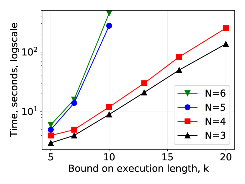
(a) Bounded model checking.

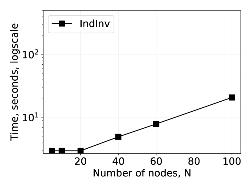
(b) Inductive invariant checking.

Figure 5: Checking $TypeOK\land SafeInv$ using apalache.

We cannot directly check the property $\mathit{Quiescence}$ with apalache, as it is written as a temporal property. One way of doing so would be to introduce a history variable that records the sequence of states seen so far and formulate the property as a state invariant over this history. apalache offers support for this approach in the form of checking so-called trace invariants.

However, we can avoid the encoding as a trace invariant by observing that the property $Quiescence$ can be verified by checking that the action invariant $terminated\Rightarrow terminated^{\prime}$ holds for all transitions taken from the reachable states. Since we have shown that $\mathit{IndInv}$ is an inductive invariant, it suffices to use apalache to check the following:

$$IndInv\land\Box[Next]_{vars}\models_{1}\Box(terminated\Rightarrow terminated^{\prime})$$ (3)

It takes apalache 3 seconds and 11 seconds to show that property (3) holds for $N=4$ and $N=100$, respectively.

3.3 Theorem Proving Using tlaps

Model checking is invaluable for finding errors, and the counter-examples computed in the case of property violations help designers understand their root cause. However, it is restricted to the verification of finite instances, and it suffers from combinatorial explosion. The TLA⁺ Proof System (tlaps) [2] can be used to prove properties of arbitrary instances of a specification. The effort is independent of the size of the state space, but it requires the user to write a proof, which is then checked by the system.

tlaps does not implement a foundational proof calculus for TLA⁺, but relies on automatic back-end provers to establish individual proof steps. Correspondingly, TLA⁺ proofs are written as a collection of steps that together entail the overall theorem. A proof step may be discharged directly by a back-end, or it may recursively be proved as the consequence of lower-level steps, leading to a hierarchical proof format [12]. The proof of an inductive invariant such as $TypeOK$ is written as follows.

$$\begin{array}[t]{@{}l@{}}\mbox{\sc theorem}\ TypeCorrect\ \mathrel{\smash{\stackrel{{\scriptstyle\scriptscriptstyle\Delta}}{{=}}}}\ Spec\Rightarrow\Box TypeOK\\ \langle 1\rangle 1.\ Init\Rightarrow TypeOK\\ \langle 1\rangle 2.\ TypeOK\land[Next]_{vars}\Rightarrow TypeOK^{\prime}\\ \langle 1\rangle 3.\ \mbox{\sc qed}\quad\mbox{\sc by}\ \langle 1\rangle 1,\,\langle 1\rangle 2,\,\textsc{ptl}\ \mbox{\sc def}\ Spec\end{array}$$

It consists of three top-level steps $\langle 1\rangle 1$ – $\langle 1\rangle 3$. The first two steps assert that the initial condition implies the invariant, and that the invariant is preserved by any transition allowed by $[Next]_{vars}$. The final qed step corresponds to proving the theorem, assuming the preceding steps could be proved. The by clause directs tlaps to check the proof of this step by invoking the ptl back-end (for “propositional temporal logic”), assuming steps $\langle 1\rangle 1$ and $\langle 1\rangle 2$, and expanding the definition of formula $Spec$. ptl can discharge this proof obligation, which essentially corresponds to an application of the proof rule

$$\begin{array}[]{@{}c}I\Rightarrow J\qquad J\land[N]_{v}\Rightarrow J^{\prime}\\ \hline\cr I\land\Box[N]_{v}\Rightarrow\Box J\end{array}$$

of temporal logic. By relying on the ptl back-end, which implements a decision procedure for linear-time temporal logic, the user does not have to indicate a specific proof rule, and tlaps can discharge more complex steps involving temporal logic.

In order to complete the proof of the theorem, we must provide proofs for steps $\langle 1\rangle 1$ and $\langle 1\rangle 2$. These steps assert (the validity of) a state and an action formula, respectively, and therefore do not require temporal logic. The first step can be proved by invoking the assumption $NAssumption$ and expanding the definitions of $Init$, $TypeOK$, and the defined operators used therein. The second step requires some more interaction and is decomposed into one sub-proof per disjunct in the definition of $Next$. The TLA⁺ Toolbox provides an assistant for such syntactic decompositions. The proofs of the invariant $Safe$ and of the safety property $Quiescence$ are similar, but they also use theorem $TypeCorrect$ in order to introduce predicate $TypeOK$ as an assumption.

The proof of the liveness property makes use of the fairness hypothesis that appears as part of the specification. Since the fairness formula is defined in terms of enabled (cf. Sect. 2), we first prove a lemma that reduces the relevant enabledness condition to a simple state predicate.

$$\begin{array}[t]{@{}l@{}}\mbox{\sc lemma}\ EnabledDT\ \mathrel{\smash{\stackrel{{\scriptstyle\scriptscriptstyle\Delta}}{{=}}}}\\ \quad\begin{array}[t]{@{}l@{\ }l@{}}\mbox{\sc assume}&TypeOK\\ \mbox{\sc prove}&(\mbox{\sc enabled}~{}\langle DetectTermination\rangle_{vars})\\ &\Leftrightarrow(terminated\land\lnot termDetect)\end{array}\end{array}$$

The proof of this lemma makes use of specific directives for reasoning about enabled provided by tlaps. The proof of the liveness property is then finished in a few lines of interaction:

$$\begin{array}[t]{@{}l@{}}\mbox{\sc theorem}\ Liveness\ \mathrel{\smash{\stackrel{{\scriptstyle\scriptscriptstyle\Delta}}{{=}}}}\ Spec\Rightarrow Live\\ \begin{array}[t]{@{}l@{\ }l@{}}\langle 1\rangle.&\textsc{define}\ P\ \mathrel{\smash{\stackrel{{\scriptstyle\scriptscriptstyle\Delta}}{{=}}}}\ terminated\land\lnot termDetect\\ \langle 1\rangle 1.&TypeOK\land P\land[Next]_{vars}\Rightarrow P^{\prime}\lor termDetect^{\prime}\\ \langle 1\rangle 2.&TypeOK\land P\land\langle DetectTermination\rangle_{vars}\Rightarrow termDetect^{\prime}\\ \langle 1\rangle 3.&TypeOK\land P\Rightarrow\mbox{\sc enabled}~{}\langle DetectTermination\rangle_{vars}\\ \langle 1\rangle 4.&\mbox{\sc qed}\quad\mbox{\sc by}\ \langle 1\rangle 1,\ \langle 1\rangle 2,\ \langle 1\rangle 3,\ TypeCorrect,\ \textsc{ptl}\ \mbox{\sc def}\ Spec,\ Live\end{array}\end{array}$$

The first two steps are proved by expanding the required definitions, the third step is a consequence of lemma $EnabledDT$, and the final step follows from the preceding ones, and theorem $TypeCorrect$, by propositional temporal reasoning. More complex cases would typically require induction over a well-founded ordering, which is supported by a standard library of TLA⁺ lemmas.

4 Safra’s Algorithm for Termination Detection

In his note EWD 998 [5], Dijkstra describes an algorithm due to Safra for detecting termination on a ring of processes. Safra’s algorithm extends a simpler algorithm due to Dijkstra, described in note EWD 840 [6], which assumes that message passing between processes is instantaneous. In both algorithms, node $0$ plays the role of a master node that will detect global termination.

In addition to the activation status and message counter represented by the variables $active$ and $pending$ introduced for the state machine of Sect. 2, each node now has a color (white or black) and maintains an integer counter that represents the difference between the numbers of messages it has sent and received during the execution. In addition, a token circulates on the ring whose attributes are its color $token.c$, its position $token.p$ (i.e., the number of the node that the token is currently at), and an integer counter $token.q$ that represents the sum of the counter values of the nodes visited so far. Safra’s algorithm does not have the variable $termDetect$.

Informally, the algorithm relies on the idea that when the system has globaly terminated, each node is locally inactive and the sum of the differences between sent and received messages is $0$. By visiting each node, checking its activation status and accumulating the counter values, the token reports these conditions to the master node. Colors are used in order to rule out false positives: nodes color themselves black at message reception (i.e., when they may have become active again), and the token becomes black when it passes a black node. A round in which a black token returns to node $0$ is deemed inconclusive.

Formally, the algorithm is described by a state machine. The initial values of each node’s activation status and color are arbitrary, all node counters are $0$, and there are no pending messages. The token is initially black (ensuring that it will perform at least one full round of the ring), and its initial counter value is $0$. The token can be located at any of the nodes. The transitions of the algorithm are as follows.

$InitiateProbe.$

Node $0$ may initiate a new round of the token when it holds the token (i.e., $token.p=0$) and when the previous round did not detect termination: either the token is black, node $0$ is black, or the sum of the counter of node $0$ and $token.q$ is positive. Node $0$ transfers a fresh white token to its neighbor node (i.e., $token.p=N-1$, $token.c=white$, and $token.q=0$) and repaints itself white.

$PassToken.$

A non-zero node $i$ may pass the token to its neighbor when it holds the token (i.e., $token.p=i$) and when it is inactive. After the transition, $token.p$ will be $i-1$, $token.q$ is augmented by node $i$’s counter value, and the token will be black if node $i$ is black or if it was already black, whereas node $i$ becomes white.

$SendMsg.$

This action is similar to the corresponding action of the abstract state machine, except that the sender’s counter value is incremented by $1$.

$RcvMsg.$

Again, this action is similar to the corresponding action of the abstract state machine. However, the receiver’s counter value is decremented by $1$, and the receiver becomes black.

$Terminate.$

This action is analogous to the corresponding action of the abstract state machine.

Node $0$ declares global termination when it is inactive, has no pending messages, holds a white token, its color is white, and the sum of $token.q$ and its own counter value is $0$. A TLA⁺ specification of the algorithm is available online [9].

5 Analyzing Safra’s Algorithm

As for the high-level specification of Section 2, we use the model checkers tlc and apalache to gain confidence in the correctness of the algorithm by checking its properties for small instances, and then start writing a full correctness proof using tlaps. Instead of rechecking the elementary correctness properties introduced in Section 3, an attractive way of verifying the correctness of the algorithm in TLA⁺ is to formally relate it to the high-level algorithm by establishing refinement.

5.1 Model Checking Correctness Properties

We start by writing a type-correctness invariant for the TLA⁺ specification of Safra’s algorithm and define the predicate of termination detection as follows:

$$termDetect\ \mathrel{\smash{\stackrel{{\scriptstyle\scriptscriptstyle\Delta}}{{=}}}}\ \begin{array}[t]{@{\mbox{$\land$\ }}l@{}}token.p=0\land token.c=\text{{``white''}}\\ color[0]=\text{{``white''}}\land\lnot active[0]\land pending[0]=0\\ token.q+counter[0]=0\end{array}$$

We use tlc to verify type correctness, as well as the properties $Safe$, $Live$, and $Quiescence$ introduced in Sect. 3, for fixed values of $N$. Again, we need a state constraint for bounding the number $K$ of pending messages at each node, but also the maximum counter values $C$ and token counter $Q$. The state space of this specification is significantly larger than that of the higher-level model: fixing $N=3$, $K=C=3$ and $Q=9$, tlc finds 1.3 million distinct states and requires 42 seconds on a desktop-class machine. For $N=4$ and the same bounds for the other parameters, we obtain 219 million distinct states, and tlc requires about 50 minutes. While tlc scales to multiple cores and can, e.g., verify safety of EWD998 for $N=4$ on a machine with 32 cores and 64 GB of memory in around 10 minutes, it would be hopeless to model check the specification for larger values such as $N=6$ in reasonable time.

Experience indicates that by exhaustively checking all reachable states, including corner cases that would arise very rarely in actual executions of the algorithm, model checking finds errors in small instances of a specification. Choosing suitable parameter values is a matter of engineering judgment. For example, an error introduced into the definition of action $PassToken$ such that the token adopts the color of the visited node, independently of the current token color, is found by tlc when $N\geq 4$, but the definition is correct for $N\leq 3$.

If exhaustive model-checking is infeasible due to the size of the state space, tlc can verify safety and liveness properties on randomly generated behaviors. Since randomized state exploration has no notion of state-space coverage, tlc runs until either it finds a violation, is manually stopped, or up to a given resource limit. Because randomized state exploration is an embarrassingly parallel problem, it scales with the number of available cores.

To illustrate the effectiveness of randomized state exploration with tlc, we separately introduced six bugs in the specification of Safra’s algorithm that we observed while teaching TLA⁺ classes. Beyond the previously mentioned bug of not taking into account the token color when non-initiator nodes pass the token, we initialize the token to white, allow an active node to pass the token, omit to whiten a node that passes the token, or prevent the initiator from initiating a new token round when its color is black. Half of these bugs violate property $Inv$, while the other half violate $TD!Spec$ (see below). With the parameter value fixed to $N=7$ and no state constraint, randomized state exploration, with a resource limit of 2 to 3 seconds and for behaviors of length up to 100 states, finds violations of $Inv$ and $TD!Spec$ in the majority of runs for any of the six bugs. Thus, the minimal resource usage makes it feasible, and the high likelihood of findings bugs makes it desirable to automatically run randomized state exploration repeatedly in the background while writing specifications. Users can run randomized state exploration with the Visual Studio Code Extension whenever its editors are saved. Once a spec has matured and randomized state exploration stops finding bugs, users can switch to exhaustive model-checking.

For more complex specifications, the likelihood of finding bugs with repeated, brief randomized state exploration can usually be increased further. If a candidate inductive invariant $IndInv$ is known, using it as the initial condition makes tlc explore states that are located at arbitrary depths in the state space. Should the set of all states defined by $IndInv$ be too large or even infinite, tlc can randomly select a subset from that set with the help of operators defined in the standard $Randomization$ module. This technique is described in more detail as part of a note on validating candidates for inductive invariants with tlc [14].

apalache again is particularly useful when it comes to checking inductive invariants. Dijkstra’s note [5] introduces the following inductive invariant $Inv$ (written in TLA⁺):

$$\begin{array}[t]{@{}l@{\ }l@{}}Sum(f,S)&\mathrel{\smash{\stackrel{{\scriptstyle\scriptscriptstyle\Delta}}{{=}}}}\ FoldFunctionOnSet(+,0,f,S)\\ Rng(a,b)&\mathrel{\smash{\stackrel{{\scriptstyle\scriptscriptstyle\Delta}}{{=}}}}\ \{i\in Node:a\leq i\land i\leq b\}\\ Inv&\mathrel{\smash{\stackrel{{\scriptstyle\scriptscriptstyle\Delta}}{{=}}}}\ \begin{array}[t]{@{\mbox{$\land$\ }}l@{}}Sum(pending,Node)=Sum(counter,Node)\\ \begin{array}[t]{@{\mbox{$\lor$\ }}l@{}}\begin{array}[t]{@{\mbox{$\land$\ }}l@{}}\forall i\in Rng(token.p+1,N-1):active[i]=\textsc{false}\\ token.q=Sum(counter,Rng(token.p+1,N-1))\end{array}\\ Sum(counter,Rng(0,token.p))+token.q>0\\ \exists i\in Rng(0,token.p):color[i]=\text{{``black''}}\\ token.c=\text{{``black''}}\end{array}\end{array}\end{array}$$

The expression $Sum(f,S)$ represents the sum of $f[x]$ for all $x\in S$; it is defined in terms of the operator $FoldFunctionOnSet$ from the TLA⁺ Community Modules [10], a collection of useful libraries for use with TLA⁺.

As explained in Sect. 3.2, we can use apalache to check that $Inv$ is indeed an inductive invariant for finite instances of the specification. For $N=4$, this takes 11 seconds. It is not hard to see that $Inv$, together with predicate $termDetect$, implies $terminated$. Indeed, $termDetect$ implies that the three final disjuncts of the invariant are false, hence the first disjunct must be true. Thus, all nodes are inactive, and $token.q$ equals the sum of the counter values of nodes $1\,..\,N-1$. By $termDetect$, it follows that the sum of the counter values of all nodes must be $0$, and by the first conjunct of $Inv$ it follows that there are no pending messages at any node, hence $terminated$ is true.

5.2 Safra’s Algorithm Implements Termination Detection

Instead of verifying the TLA⁺ specification of Safra’s algorithm against correctness properties such as $Safe$ and $Live$, we can show that it implements the high-level state machine of Sect. 2. It then follows that the properties verified for that state machine are “inherited” by the low-level specification. Since in TLA⁺, refinement is implication, this assertion can be stated by inserting the following lines in the module representing Safra’s algorithm:

$$\begin{array}[t]{@{}l@{}}TD\ \mathrel{\smash{\stackrel{{\scriptstyle\scriptscriptstyle\Delta}}{{=}}}}\ \mbox{\sc instance}\ AsynchronousTerminationDetection\\ \mbox{\sc theorem}\ Refinement\ \mathrel{\smash{\stackrel{{\scriptstyle\scriptscriptstyle\Delta}}{{=}}}}\ Spec\Rightarrow TD!Spec\end{array}$$

The first line declares an instance $TD$ of the high-level specification in which the constant parameter $N$ and the variable parameters $active$, $pending$ and $termDetect$ are instantiated by the expressions of the same name in the specification of Safra’s algorithm. Theorem $Refinement$ asserts that every run of $Spec$ (the specification of Safra’s algorithm) also satisfies $TD!Spec$, defined in Fig. 2.

tlc can reasonably verify refinement for values of $N<5$, and with a similar state constraint as before, simply by indicating $TD!Spec$ as the temporal property to be checked. apalache cannot handle the fairness condition that is part of $TD!Spec$, but it can verify initialization and step simulation. Technically, this is done by checking one state invariant and one action invariant with apalache:

$$Init\land\Box[Next]_{vars} \models_{0}\Box TD!Init$$ (4)

$$TypeOK\land Inv\land\Box[Next]_{vars} \models_{1}\Box[TD!Next]_{TD!vars}$$ (5)

Checking condition (4) with the apalache machinery is equivalent to showing $\mathit{Init}\Rightarrow TD!Init$, which is needed to show the initialization property of refinement. To prove step simulation, we have to show that any transition described by $[Next]_{vars}$, starting in any reachable state of the low-level specification, simulates a high-level transition according to $[TD!Next]_{TD!vars}$. As expressed in condition (5), the previously established inductive invariants $TypeOK$ and $Inv$ are sufficient for proving step simulation.

The TLA⁺ specification of Safra’s algorithm as described in Sect. 4 can be refined further by introducing explicit message channels and node addresses. We refer readers to the modules $EWD998Chan$ and $EWD998ChanID$ [9] that contain corresponding TLA⁺ specifications for which refinement can be checked using the TLA⁺ tools.

5.3 Proving Correctness Using tlaps

After gaining confidence in the validity of our specification of Safra’s algorithm, we again use tlaps for proving its correctness for arbitrary instances. The type correctness proof is quite similar to that of the high-level specification described in Section 3.3. We also used tlaps for proving the inductive invariant $Inv$ introduced in Sect. 5.1. However, at the time of writing, no theorem libraries exist in tlaps for operators such as $FoldFunctionOnSet$, and we therefore stated elementary properties without proof, and specialized them for the derived operator $Sum$ such as

$$\begin{array}[t]{@{}l@{}}\mbox{\sc lemma}\ SumIterate\ \mathrel{\smash{\stackrel{{\scriptstyle\scriptscriptstyle\Delta}}{{=}}}}\\ \quad\begin{array}[t]{@{}l@{\ }l@{}}\mbox{\sc assume}&\textsc{new}\ fun\in[Node\rightarrow Int],\\ &\textsc{new}\ inds\in\mbox{\sc subset}\ Node,\ \textsc{new}\ e\in inds\\ \mbox{\sc prove}&Sum(fun,inds)=fun[e]+Sum(fun,inds\setminus\{e\})\end{array}\end{array}$$

The invariance proof itself was written in one person-day and required about 230 lines in the proof language of TLA⁺. The hierarchical proof style helps to focus on individual steps without having to remember the overall proof.

Based on the inductive invariant and the following lemma

$$\begin{array}[t]{@{}l@{}}\mbox{\sc lemma}\ Safety\ \mathrel{\smash{\stackrel{{\scriptstyle\scriptscriptstyle\Delta}}{{=}}}}\ TypeOK\land Inv\land termDetect\Rightarrow Termination\end{array}$$

that formalizes the argument presented at the end of Sect. 5.1, it is not hard to use tlaps for proving the safety part of the refinement relation, i.e. the implications expressed by properties (4) and (5), for arbitrary instances of the specification. The proofs of the lemma and the safety part of the refinement theorem require about 110 lines of TLA⁺ proof and were written in half a person-day.

In order to prove liveness of the algorithm, we first reduce the enabledness condition of the action for which fairness is assumed, to a simple state predicate, as we did in Sect. 3.3. We must then show that any state satisfying predicate $terminated$ must be followed by one where $termDetect$ holds. Relying on the already proved invariants, we set up a proof by contradiction and define

$$BSpec\ \mathrel{\smash{\stackrel{{\scriptstyle\scriptscriptstyle\Delta}}{{=}}}}\ \Box TypeOK\land\Box Inv\land\Box\lnot termDetect\land\Box[Next]_{vars}\land\textrm{WF}_{vars}(System)$$

where the last conjunct corresponds to the fairness assumption of the specification, in which $System$ represents the disjunction of the token-passing transitions. Informally, detecting termination may require three rounds of the token:

1. The first round brings the token back to node $0$, while $terminated$ remains true.

2. After the second round, the token is back at node $0$, all nodes are white (since no messages could be received), and $terminated$ is still true.

3. At the end of the third round, the same conditions hold, and additionally the token is white and the token counter holds the sum of the counters of the nodes in the interval $1\,..\,N-1$.

We prove a lemma corresponding to each of the rounds. For example, for the first round we assert

$$\mbox{\sc lemma}\ Round1\ \mathrel{\smash{\stackrel{{\scriptstyle\scriptscriptstyle\Delta}}{{=}}}}\ BSpec\Rightarrow(terminated\leadsto(terminated\land token.p=0))$$

The proof proceeds by induction on the current position $k$ of the node: if $k=0$, the assertion is trivial. For the case $k+1$, any step of the system either leaves the token at node $k+1$ or brings it to node $k$. Moreover, the token-passing transition from node $k+1$ is enabled, and it takes the token to node $k$.

The statements and proofs of the two other lemmas are similar. Finally, the post-condition of the third round, together with $Inv$, implies $termDetect$, concluding the proof. As a corollary, we can finish the refinement proof: we showed in Sect. 3.3 that the enabledness condition of $TD.DetectTermination$ corresponds to the conjunction $terminated\land\lnot termDetect$, and we just proved that this predicate cannot hold forever, implying the fairness condition. The TLA⁺ proof takes 245 lines and was written in less than one person-day, aided by the fact that the three main lemmas and their proofs are quite similar.

6 Conclusion

TLA⁺ is a language for the formal and unambiguous description of algorithms and systems. In this paper, we presented the three main tools for verifying properties of TLA⁺ specifications: the explicit-state model checker tlc, the symbolic model checker apalache, and the interactive proof assistant tlaps, at the hand of a formal specification of a non-trivial distributed algorithm. The ProB model checker can also verify TLA⁺ specifications through a translation to B [7], but we did not evaluate its use on the case study presented here. The three tools that we considered have complementary strengths and weaknesses. They offer various degrees of proof power in exchange for manual effort or computational resources. Whereas tlc is essentially a push-button tool, tlaps requires significant user effort for inventing a proof. Likewise, apalache can sometimes prove invariants of specifications that have significantly larger (or even infinite) state spaces than tlc can handle, but it requires human ingenuity to find an inductive invariant. Hence, we advocate the following basic workflow.

Since errors in specifications are usually found for small instances, it is easiest to start by using tlc for checking basic invariant properties. The same properties can also be checked using apalache for short execution prefixes. However, apalache really shines for checking inductive (state and action) invariants since doing so only requires considering a single transition. Once reasonable confidence has been obtained for safety properties, liveness properties can be verified using tlc. One potential pitfall here is that the use of a state constraint may mask non-progress cycles in which some variable value exceeds the admissible bounds. Both model checkers suffer from combinatorial explosion; for apalache the length of the execution prefixes that need to be examined tends to be the limiting factor. For very large state spaces, tlc provides support for randomized state exploration, which empirically tends to find bugs with good success when exhaustive exploration fails. When model checking finds no more errors and even more confidence is required, one can start writing a proof and check it using tlaps. In this way, properties of arbitrary instances can be verified, at the expense of human effort that can become substantial in the presence of complex formulas.

All three tools accept the same input language TLA⁺. Whereas apalache requires writing typing annotations for state variables and certain operator definitions, these are usually not very difficult to come up with. Not surprisingly, the tools pose additional restrictions on the input specifications. For example:

1. tlc rejects action formulas of the form $x^{\prime}\in S$ when $S$ is an infinite set, and no unique value has been determined for the variable $x^{\prime}$ by an earlier conjunct: in this case, the formula would require tlc to enumerate an infinite set. However, the user can override operator definitions such as $S$ during model-checking without modifying the original specification.

2. apalache has recently dropped support for recursive operators and functions in favor of fold operations, e.g., $\mathit{FoldSet}$ and $\mathit{FoldFunction}$. Folding a set $S$ of bounded cardinality, that is, $|S|\leq n$, for some $n$, needs up to $n$ iterations, which is easy to encode in SMT as opposed to general recursion.

3. tlaps currently does not handle recursive operator definitions, and support for proving liveness properties has only recently been added. In practice, reasoning about operators that are not supported natively by its backends requires well-developed theorem libraries.

Despite these limitations, all three tools share a large common fragment of TLA⁺. This ability to use different tools for the same specification is extremely valuable in practice, for example for using the model checkers to verify a putative inductive invariant in the middle of writing an interactive proof.

Future work should focus on improving the capabilities of each tool. Although tlc is quite mature, it could benefit from better parallelization of liveness checking. Recent work has focused on improved presentation of counter-examples, including their visualization and animation [15], and on randomized exploration of state spaces. For apalache, alternative encodings of bounded verification problems as SMT problems could help with performance degradation when considering longer execution prefixes. It would also be useful to lift the current restriction to the verification of safety properties and consider bounded verification of liveness properties. tlaps users would appreciate better automation, such as the tool being able to indicate which operator definitions should be expanded, better support for higher-order problems, and for verifying liveness properties. The IDEs could help with using the tools synergistically, such as starting an exploratory model checking run that corresponds to a given step in a proof.

Besides the work on verifying properties of formal specifications, there is interest in relating TLA⁺ specifications to system implementations. The two main lines of research are model-based test case generation from formal specifications and trace validation, in which the specification serves as a monitor for supervising an implementation. Davis et al. [3] present an interesting real-life case study, in which trace validation was found to be particularly successful.

References

- [1] Biere, A., Cimatti, A., Clarke, E.M., Zhu, Y.: Symbolic model checking without BDDs. In: TACAS. LNCS, vol. 1579, pp. 193–207 (1999)
- [2] Cousineau, D., Doligez, D., Lamport, L., Merz, S., Ricketts, D., Vanzetto, H.: TLA+ proofs. In: Giannakopoulou, D., Méry, D. (eds.) 18th Intl. Symp. Formal Methods (FM 2012). LNCS, vol. 7436, pp. 147–154. Springer, Paris, France (2012)
- [3] Davis, A.J.J., Hirschhorn, M., Schvimer, J.: Extreme modelling in practice. Proc. VLDB Endow. 13(9), 1346–1358 (2020)
- [4] de Moura, L.M., Bjørner, N.: Z3: An efficient SMT solver. In: Ramakrishnan, C.R., Rehof, J. (eds.) TACAS 2008. LNCS, vol. 4963, pp. 337–340. Springer, Budapest, Hungary (2008)
- [5] Dijkstra, E.W.: Shmuel Safra’s version of termination detection (1987), available online at https://www.cs.utexas.edu/users/EWD/ewd09xx/EWD998.PDF
- [6] Dijkstra, E.W., W.H.J.Feijen, van Gasteren, A.: Derivation of a termination detection algorithm for distributed computations. Inf. Proc. Letters 16, 217–219 (1983)
- [7] Hansen, D., Leuschel, M.: Translating TLA+ to B for validation with ProB. In: Derrick, J., Gnesi, S., Latella, D., Treharne, H. (eds.) 9th Intl. Conf. Integrated Formal Methods (iFM 2012). LNCS, vol. 7321, pp. 24–38. Springer, Pisa, Italy (2012)
- [8] Konnov, I., Kukovec, J., Tran, T.: TLA+ model checking made symbolic. Proc. ACM Program. Lang. 3(OOPSLA), 123:1–123:30 (2019)
- [9] Konnov, I., Kuppe, M., Merz, S.: TLA+ specifications of EWD998 (2021), https://github.com/tlaplus/Examples/tree/ISoLA2022/specifications/ewd998
- [10] Kuppe, M.A., Merz, S., Rafael Feodrippe, P., Lamport, L., Schultz, W., Fernandes, A., Ryndzionek, M., Konnov, I., Halterman, J., Wayne, H., Jobvs: TLA+ Community Modules, https://github.com/tlaplus/CommunityModules
- [11] Kuppe, M.A., Lamport, L., Ricketts, D.: The TLA+ toolbox. In: Monahan, R., Prevosto, V., Proença, J. (eds.) Fifth Workshop on Formal Integrated Development Environment (F-IDE). EPTCS, vol. 310, pp. 50–62. Porto, Portugal (2019)
- [12] Lamport, L.: How to write a proof. American Mathematical Monthly 102(7), 600–608 (1995)
- [13] Lamport, L.: Specifying Systems. Addison-Wesley, Boston, Mass. (2002)
- [14] Lamport, L.: Using TLC to check inductive invariance (2018), https://lamport.azurewebsites.net/tla/inductive-invariant.pdf
- [15] Schultz, W.: An Animation Module for TLA+ (2018), https://easychair.org/smart-slide/slide/8V76
- [16] Yu, Y., Manolios, P., Lamport, L.: Model checking TLA+ specifications. In: Pierre, L., Kropf, T. (eds.) Correct Hardware Design and Verification Methods (CHARME’99). LNCS, vol. 1703, pp. 54–66. Springer Verlag, Bad Herrenalb, Germany (1999)