Experimental study of Neural ODE training with adaptive solver for dynamical systems modeling

Abstract

Neural Ordinary Differential Equations (ODEs) was recently introduced as a new family of neural network models, which relies on black-box ODE solvers for inference and training. Some ODE solvers called adaptive can adapt their evaluation strategy depending on the complexity of the problem at hand, opening great perspectives in machine learning. However, this paper describes a simple set of experiments to show why adaptive solvers cannot be seamlessly leveraged as a black-box for dynamical systems modelling. By taking the Lorenz’63 system as a showcase, we show that a naive application of the Fehlberg’s method does not yield the expected results. Moreover, a simple workaround is proposed that assumes a tighter interaction between the solver and the training strategy.

1 Introduction

A recent line of work has explored the interpretation of residual neural networks [9] as a parameter estimation problem of nonlinear dynamical systems [8, 4, 12]. Reconsidering this architecture as an Euler discretization of a continuous system yields to the trend around Neural Ordinary Differential Equation [2]. This new perspective on deep learning holds the promise to leverage the decades of research on numerical methods. This can have many benefits such as parameter efficiency and accurate time-series modeling, among others.

Numerical solvers for ODE act as a bridge between the continuous time dynamical system and its discrete counterpart that builds the deep neural network. As introduced by [2], modern ODE solvers can provide important guarantees about the approximation error while adapting their step size used for integration. Therefore the cost of evaluating a model scales with problem complexity, in theory at least. This paper address this question empirically using the Lorenz’63 system described in section 2 as a testbed for dynamical systems modelling. Our neural ODE framework relies on Fehlberg’s integration method which proposes a strategy of step-size adaptation as summarized in 2.2. A first round of experiments is reported in 3 to assess how this adaptive method impacts the inference of the model and the training process. We show empirically that the adaptive strategy is in fact ignored. In section 4, a simple solution, called Fehlberg’s training, is introduced that requires to open the black-box of the solver for a tighter interaction with the training process.

2 Neural ODE applied to the Lorenz’63

To empirically analyse how an adaptive solver interacts with the training procedure of a neural ODE model, we consider the Lorenz’63 system [11]. This “butterfly” attractor was originally introduced to mimic the thermal convection in the atmosphere, but nowadays this chaotic system is broadly used as a benchmark for time series modeling. See for instance [13, 1, 7, 3, 6] just to name a few recent work. Consider a point $\mathbf{x}\in\mathbb{R}^{3}$ with its three coordinates $x_{1},x_{2},x_{3}$. The Lorenz’63 system consists of three coupled nonlinear ODEs:

$$\dot{x}_{1}=\frac{dx_{1}}{dt}=\sigma(x_{2}-x_{1}),\phantom{5ex}\dot{x}_{2}=x_{1}(\rho-x_{3})-x_{1},\phantom{5ex}\dot{x}_{3}=x_{1}x_{2}-\beta x_{3}.$$ (1)

In this work we consider the standard setting ($\beta=8/3,\ \sigma=10,\ \rho=28$), such that the solution exhibits a chaotic regime. The dataset generation uses the explicit Runge-Kutta (RK) method of order 5(4) with the Dormand-Prince step-size adaptation in order to get an accurate integration.

2.1 Neural ODE model

The goal is to learn a generative model of this attractor, given a training set $\mathcal{D}=(\tilde{\mathbf{x}}_{i})_{i=1}^{N}$ made of $N$ examples. For time series modelling, recurrent architectures [13, 3] or physically inspired models [7] are often considered with success. However, the system understudy derives from an ODE and Neural ODE is also a well suited framework to consider. The main idea is to learn the dynamics underlying the generation of $\mathcal{D}$. The neural network aims at learning $\dot{\mathbf{x}}=f_{\boldsymbol{\theta}}(\mathbf{x})$, where $f_{\boldsymbol{\theta}}$ is an arbitrary architecture defined by its set of parameters $\boldsymbol{\theta}$. Inference with Neural ODE thus requires a numerical solver denoted by ODE_Solve to compute the output. In our case, we consider the prediction task of the point ${\mathbf{x}}_{i}$ at time $i$, given the previous training point $\tilde{\mathbf{x}}_{i-1}$, such that ${\mathbf{x}}_{i}=\textrm{ODE\_Solve}(f_{\boldsymbol{\theta}},\tilde{\mathbf{x}}_{i})$. The model is learnt by minimizing the Mean-Squared-Error: $\mathcal{L}(\boldsymbol{\theta},\mathcal{D})=\sum_{i=1}^{N}||\tilde{\mathbf{x}}_{i}-\mathbf{x}_{i}||^{2}$.

An advantage of Neural ODE is the choice of the solver and especially the possibility to adapt the step size depending on the problem complexity. In this paper, we focus on the Fehlberg’s 3(2) method [5], for its simplicity of exposition, since our goal is to analyse how the interaction between the solver and the training process.

2.2 Fehlberg’s method under the hood

In general, variable step size methods all rely on the same idea: for an inference step, try two different algorithms, giving two different hypotheses called $A_{1}$ and $A_{2}$. The two algorithms are chosen so that: i) the difference $A_{2}-A_{1}$ provides an approximate of the local truncation error; and ii) both algorithms use at most the same evaluations of $f_{\boldsymbol{\theta}}$ to limit the computational cost. In our case, the method requires three evaluations of $f_{\boldsymbol{\theta}}$ defined as follows for the step size denoted by $h$:

$$f_{1}=f_{\boldsymbol{\theta}}(\mathbf{x}_{i}),\phantom{5ex}f_{2}=f_{\boldsymbol{\theta}}(\mathbf{x}_{i}+hf_{1}),\phantom{5ex}f_{3}=f_{\boldsymbol{\theta}}(\mathbf{x}_{i}+\frac{h}{4}[f_{1}+f_{2}])$$

With these three evaluations, two approximations for the next point can be derived:

$$A_{1}=\mathbf{x}_{i}+\frac{h}{2}[f_{1}+f_{2}]\text{ (RK2 method), and }A_{2}=\mathbf{x}_{i}+\frac{h}{6}[f_{1}+f_{2}+4f_{3}]\text{ (RK3).}$$ (2)

Considering the property of these two algorithms, we can estimate the following error rate:

$$r=\frac{|A_{1}-A_{2}|}{h}\approx Kh^{2}$$ (3)

If this error rate exceeds a chosen tolerance $\epsilon$, the hypothesis $A_{2}$ is rejected and we need to restart the computation with a new step size: $h^{\prime}=S\times h\sqrt{\epsilon/r},$ with $S$ a safety factor. The initial time step is $h=1$, and we use the default value: $S=0.9$ and $\epsilon=0.1$. This strategy allows the model to increase the number of integration steps when predicting the next point $\mathbf{x}_{i+1}$ to adapt the expected precision given $r$.

3 First round of experiments

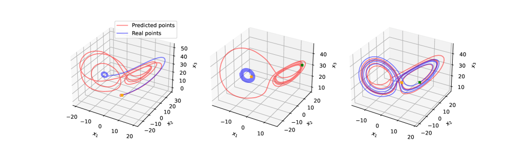
Figure 1: The trajectories predicted after a regular training, using the Fehlberg’s solver as a black box. Each figure depicts a different time slice of the generated trajectory and of the original training data: from 0 to 600, 600 to 1200 and 2000 to 2600.

For the first set of experiments, a simple ODE model is trained with L-BFGS [10] wrapped in the Fehlberg’s method. The neural network $f_{\boldsymbol{\theta}}$ is a simple feed-forward architecture with two hidden layer of size $50$ and ReLu activation. The trained model is then used to generate data, starting from the same initial condition and the figure 1 shows the results obtained for different time windows. This task differs from the training phase, and we can see that the model fails to accurately reproduce the trajectory of the original dynamical system. Especially the beginning of the trajectory greatly differs. The combination of the accumulated truncation errors with the chaoticity of the Lorenz’63 leads to too challenging generation task while the model can capture some important features like the “butterfly” aspect. The same trend is observed on the development set.

Figure 2: Time evolution of (from left to right and top to bottom): the MSE, the evolution of $x_{1}$, the MSE w.r.t the true ODE of Lorenz’63, and the number of steps.

This disappointing performance can be explain by the figure 2 which represents the time evolution of different quantities of interest. The evolution of the MSE highlights its limitation to evaluate chaotic system modelling: errors on the first points are small in terms of MSE, while inducing an important time distortion later. This can be observed by comparing the trajectories of the first component $x_{1}$. Since we have access to the physical system, we can measure another MSE by comparing each point $\mathbf{x}_{i}$ generated by the model, with what would be generated by the Lorenz ODE of equation 1 from the previous predicted point or $\mathbf{x}_{i}^{*}=Lorenz(\mathbf{x}_{i-1})$. This quantity is the third time series represented in figure 2 and provides a different insight on the performance. More importantly, the last plot monitors the number of integration steps for each prediction. In most of the case, this number is stuck to 1, showing a very limited usage of the step size adaption.

To further understand this fact, we investigate what happens during the training process by monitoring three different quantities measured after each epoch and represented in figure 3. The first column corresponds to the standard training method which considers the adaptive solver as a black-box as described in the seminal paper [2]. We can observe from the second row that the Fehlberg’s method accepts the vast majority of the RK3 prediction with one step, without resorting to an adaptive step size. Moreover, the step size is just slightly increased for a handful of training examples (see the third row). We can conclude that the adaptive step size is not harnessed by the Neural ODE model.

In fact, the model is randomly initialized with values around zeros, and the error estimation in equation 3 falls under $\epsilon$ in most of the case, and whatever the input of the model is. A first workaround would be to explore a tailored initialization scheme, with the goal of increasing this initial estimate. Another workaround consists in lowering the tolerance factor $\epsilon$ to let the Felhberg’s method reject more hypotheses and therefore adapt the step size more frequently. However, this introduces a new hyperparameter to tune.

4 Fehlberg’s training

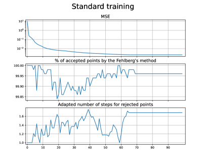
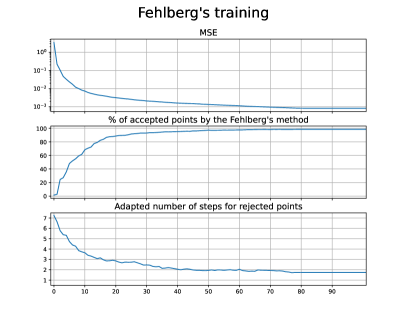
Figure 3: Time evolution for two training conditions of: the MSE loss; the percentage of accepted hypotheses $A_{2}$; the new number of steps for the rejected hypotheses (before rounding).

In this paper, we propose another solution which modifies the training procedure. The idea derives from the Fehlberg’s method by simply changing how the local truncation error is estimated. Let us consider equation 2 defining the error rate. When predicting the value $\mathbf{x}_{i}$ from $\tilde{\mathbf{x}}_{i-1}$, we can use directly the target value $\tilde{\mathbf{x}}_{i}$, which is available during training, instead of the raw estimate $A_{1}$ given by the Heun’s method (aka RK2). The basic hypothesis $A_{2}$ is still obtained with one step of RK3. Given this modified error rate, the step-size adaptation remains unchanged. This new method greatly impacts the training process. On the second column of the figure 3, we observe a very different trend: the proportion of accepted hypotheses starts at 0 and progressively increases to reach approximately 98%. For the rejected hypotheses, the new number of steps (before rounding) starts at the high value of $7$ and affects all the training examples: after the random initialization of $f_{\boldsymbol{\theta}}$, all the training examples are considered as difficult, while the high number of steps multiplies the amount of updates for $\boldsymbol{\theta}$. Then the number of steps smoothly decreases to converge to a value just under $2$ and affects about 2% of the training points. We can conclude that the new training scheme allows the Neural ODE model to really leverage the adaptive step size strategy. Of course it requires to interact with the adaptive solver, but without adding new hyperparameters or trade-offs. See Appendix C for more figures and comparisons.

5 Conclusion

In this experimental paper, we investigated how the numerical solver interacts with the training process of a neural ODE model. We focused our work on a solver able to adapt its step size. With a simple experimental setup, the results showed that using a solver as black box drastically hinders the promise of the adaptive strategy for the step size. This is a real issue to model more complex dynamical systems. We proposed a simple yet efficient solution that requires a tighter interaction between the solver and the training process. With our results, it will be possible to tackle more challenging tasks and while we focused on generative models for time series forecasting, it could be useful to extend our approach to classification tasks.

Aknowledgment: This work was funded by the French National Research Agency (ANR SPEED-20-CE23-0025). Thanks to Clément Royer for his help.

Appendix A Experimental setup

For the experiments reported in the paper, two datasets were generated, one for training and one for testing. Each of them consists in a trajectory of 5000 points.

A.1 Optimization

The training process is carried out in batch mode with the L-BFGS optimizer with the default setting:

• The initial learning rate is set by default to 1. However, L-BFGS quickly reconsider this value through many function evaluation.

• The number of iterations per optimization step is set to 20. It means that one epoch of the batch training is not comparable with other optimization algorithms like gradient descent or ADAM.

• The number of function evaluations per optimization step is 25, and the tolerance factors are set to $10^{-5}$ for the gradient, and $10^{-9}$ for the tolerance on function value changes.

• The history size is limited to 100 and the optimizer uses a line search (see [10]).

For the Fehlberg’s method, we use our own implementation without using the adjoint method.

A.2 Batch training

With Neural ODE, $f_{\boldsymbol{\theta}}$ represents the elementary block. The inference step consists building on the fly the whole network, depending on how the solver proceeds to predict the output. For instance, with the Euler method, the whole network is very similar to the ResNet architecture [9, 8, 12]. With the Fehlberg’s method, the step size is adapted for each training example, meaning that the whole network (and its computational graph) is different. This is an obstacle for mini-batch or batch training. However, online training drastically increase the computational time. As a trade-off, we propose the following procedure for each (mini) batch:

• compute $A_{1},A_{2}$, and $r$;

• for the “accepted” subpart, such as $r<\epsilon$, return $A_{2}$;

• for the remaining part, compute the new step size $h^{\prime}$ for each training example and keep the minimum value, clipping the value at $1/10$, which corresponds to $10$ steps of integration. Recompute $A_{2}$ with this value.

With this procedure, we can therefore benefit from batch training and the choice of the minimum value is a way to promote small step size.

Appendix B Impact of $\epsilon$

The threshold $\epsilon$ introduced in section 3 can mitigate the number of accepted and rejected hypotheses during the Fehlberg’s integration. To increase the number of rejected hypotheses, we can try to lower $\epsilon$. To see how this hyperparameter can impact the learning process, we train the same model with different values of $\epsilon$. In the main part of the paper, the first column of figure 3 shows how the regular training evolves with $\epsilon=0.1$ (the default value). Let us consider lower values starting with $\epsilon=0.05$ in figure 4. In this case, it does not really promote the step size adaptation. If we lower $\epsilon$ to $0.01$ as shown on the right side of figure 4, the number of accepted hypotheses per epoch decrease around $90\%$, while the number of steps is rounded up $4$ for the rejected hypotheses.

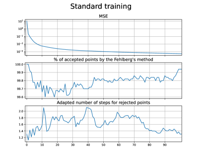
Figure 4: Time evolution for regular training with $\epsilon=0.05$ on the left, and $\epsilon=0.01$ on the right, for: the MSE loss; the percentage of accepted hypotheses $A_{2}$; the new number of steps for the rejected hypotheses (before rounding).

It is worth noticing that the $x$-axis is twice wider. The training process is longer, in terms of number of epochs, and the computation time is also augmented since $90\%$ of the training points requires 4 integration steps. However, if we look at the generation abilities, the results are really better as shown in figure 5: the generation still fails to mimic the original Lorenz for the starting points, but after the generation is really similar to the original one.

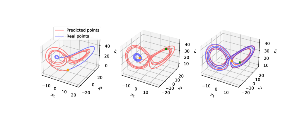
Figure 5: The trajectories predicted after a regular training with $\epsilon=0.01$, using the Fehlberg’s solver as a black box. Each figure depicts a different time slice of the generated trajectory and of the original training data: from 0 to 600, 600 to 1200 and 2000 to 2600.

Appendix C Additional figures for Fehlberg’s training

To complement the comparison of the baseline training and the Fehlberg’s training (see respectively section 3 and 4), additional figures are provided here.

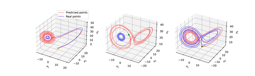
Figure 6: The trajectories predicted after the Fehlberg’s training.

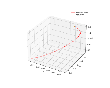
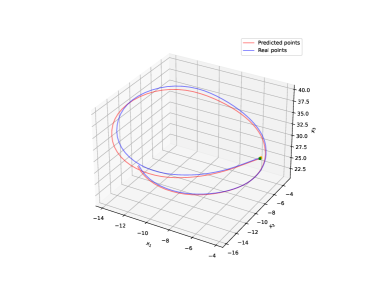
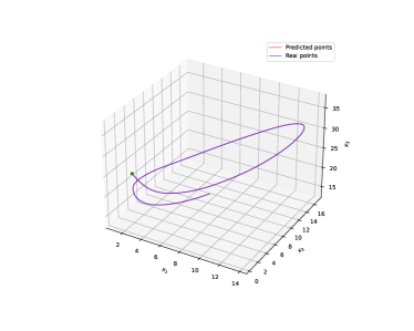
Figure 7: On the first row: the 20 first time steps of generation for the baseline and Fehlberg’s training vs the real data points. Then on the second row, the same predicted points vs the points generated by the Lorenz ODE from the predicted ones (i.e the ones used to estimate the modified MSE as described in section 3). These two figures show the errors made by the models but these errors are not affected by the chaoticity of the Lorenz. The last row shows the same two figures, but for time steps from 1000 to 1100.

References

- [1] Kathleen Champion, Bethany Lusch, J. Nathan Kutz, and Steven L. Brunton. Data-driven discovery of coordinates and governing equations. Proceedings of the National Academy of Sciences, 116(45):22445–22451, 2019.
- [2] R. T. Q. Chen, Y. Rubanova, J. Bettencourt, and D. K. Duvenaud. Neural ordinary differential equations. In Advances in Neural Information Processing Systems 31, pages 6571–6583, 2018.
- [3] Pierre Dubois, Thomas Gomez, Laurent Planckaert, and Laurent Perret. Data-driven predictions of the Lorenz system. Physica D: Nonlinear Phenomena, 408:132495, July 2020.
- [4] Weinan E. A proposal on machine learning via dynamical systems. Communications in Mathematics and Statistics, 5(1):1–11, Mar 2017.
- [5] Erwin. Fehlberg and NASA. Classical fifth-, sixth-, seventh-, and eighth-order Runge-Kutta formulas with stepsize control. NASA Technical Report. NASA, Washington, D.C., 1968.
- [6] William Gilpin. Chaos as an interpretable benchmark for forecasting and data-driven modelling. In Thirty-fifth Conference on Neural Information Processing Systems Datasets and Benchmarks Track (Round 2), 2021.
- [7] S. Greydanus, M. Dzamba, and J. Yosinski. Hamiltonian neural networks. In Advances in Neural Information Processing Systems 32, pages 15379–15389, 2019.
- [8] Eldad Haber and Lars Ruthotto. Stable architectures for deep neural networks. Inverse Problems, 34(1):014004, dec 2017.
- [9] Kaiming He, Xiangyu Zhang, Shaoqing Ren, and Jian Sun. Deep residual learning for image recognition. In The IEEE Conference on Computer Vision and Pattern Recognition, 2016.
- [10] D. C. Liu and J. Nocedal. On the limited memory BFGS method for large scale optimization. Math. Programming, 45(3, (Ser. B)):503–528, 1989.
- [11] Edward Lorenz. Deterministic nonperiodic flow. Journal of Atmospheric Sciences, 20(2):130–148, 1963.
- [12] Y. Lu, A. Zhong, Q. Li, and B. Dong. Beyond finite layer neural networks: Bridging deep architectures and numerical differential equations. In Proceedings of the 35th International Conference on Machine Learning, 2018.
- [13] Josue Nassar, Scott Linderman, Monica Bugallo, and Il Memming Park. Tree-structured recurrent switching linear dynamical systems for multi-scale modeling. In International Conference on Learning Representations, 2019.