Effective potential in non-perturbative gauge theories

Abstract

We consider a formalism to describe the false-vacuum decay of a scalar field in gauge theories in non-perturbative regimes. We find that the larger the gauge coupling with respect to the self-coupling of the scalar, the shallower the local minimum of the unstable vacuum, to the point where it disappears. This offers the possibility to obtain a consistent picture of early universe cosmology: at high temperatures, a false-vacuum decay is strongly favoured and the universe naturally evolves towards a stable state.

I Introduction

With the advent of gravitational-wave astronomy in the past few years LIGOScientific:2016lio and the Higgs boson discovery at LHC and its implication of the vacuum meta-stability Degrassi:2012ry ; Isidori:2001bm made the possibility to observe a stochastic gravitational-wave background produced from primordial first-order phase transition more concrete than ever (see, e.g, LISACosmologyWorkingGroup:2022jok and references therein). Constraints on such a stochastic Gravitational Waves background (SGWB) had been given well before the first observations of gravitational waves 2009Natur.460..990A and presently are being constantly refined across different frequencies and regions in the parameter space of the models LISACosmologyWorkingGroup:2022jok . We are currently looking for more and more accurate calculations of the false-vacuum decay rate in the myriad of beyond-the-Standard-Model theories available, ranging from scenarios described by weak perturbation theory to strongly coupled regimes for Higgs as well as gauge theories.

In this paper, we make a step further towards our understanding of false-vacuum decay using a technique useful to probe analytically the non-perturbative regime of quantum field theories Frasca:2015wva ; Frasca:2015yva ; Chaichian:2018cyv ; Frasca:2021yuu ; Frasca:2021zyn ; Frasca:2022kfy ; Frasca:2022lwp ; Frasca:2022vvp ; Calcagni:2022tls . We consider a theory with scalar and gauge fields (Sec. II) and compute the effective potential and the fluctuations for the scalar (Sec. III), finding that the height of the minima depends on the interplay between the scalar self-coupling $\lambda$ and the gauge coupling $g$. Although we work in Minkowski spacetime without gravity, these results can pave the way to a natural picture of the evolution of the early universe from an unstable to a stable vacuum state (Sec. IV).

II Model and solutions

II.1 Lagrangian

We consider the following Lagrangian:

$${\cal L}=-\frac{1}{4}F_{\mu\nu}^{a}F^{a\mu\nu}+\frac{1}{2}(\partial_{\mu}\phi-igT^{a}A_{\mu}^{a}\phi)^{2}-V(\phi)+L_{\rm GF}+L_{\rm FP},$$ (1)

where $F_{\mu\nu}^{a}=\partial_{\mu}A_{\nu}^{a}-\partial_{\nu}A^{a}_{\nu}+gf^{abc}A^{b}_{\mu}A^{c}_{\nu}$, provided that $[T^{a},T^{b}]=if^{abc}T^{c}$ with $f^{abc}$ the structure constants of the gauge group. $V(\phi)$ is the potential of the scalar field with a false vacuum. $L_{\rm GF}$ is the gauge fixing part and $L_{\rm FP}$ is the contribution of Faddeev–Popov ghosts $c$ and $\bar{c}$. We use $(+,-,-,-)$ signature.

II.2 Solutions

Let us consider the partition function

$$Z[j_{A},j_{\phi},\bar{\eta},\eta]=\int[dA][d\phi][d\bar{c}][dc]e^{i\int d^{4}xL+i\int d^{4}x[j_{A}^{a\mu}A^{a}_{\mu}+j_{\phi}\phi+\bar{\eta}^{a}c^{a}+\bar{c}^{a}\eta^{a}]}.$$ (2)

Then, we notice that

$$(\partial_{\mu}\phi-igT^{a}A_{\mu}^{a}\phi)^{2}=(\partial\phi)^{2}-2igA^{a}_{\mu}(\phi T^{a}\partial\phi)-g^{2}A_{\mu}^{a}A^{b\mu}(T^{a}\phi)(T^{b}\phi).$$ (3)

For the gauge sector, we observe that the ghost sector decouples for the correlation functions and we can consider the expansion

$$A_{\mu}^{a}[x;j]=\eta_{\mu}^{a}G_{1}(x)+\int d^{4}yG_{2\mu\nu}^{ab}(x-y)j^{b\nu}(y)+O(j^{2}).$$ (4)

Then we can write the partition function as

$$Z[j_{\phi}] = Z_{0}\int[d\phi]e^{i\int d^{4}x\left[\frac{1}{2}(\partial\phi)^{2}-V(\phi)-ig\left(-i\frac{\delta}{\delta j_{\mu}^{a}(x)}\right)(\phi T^{a}\partial\phi)-\frac{1}{2}g^{2}\left(-i\frac{\delta}{\delta j_{\mu}^{a}(x)}\right)\left(-i\frac{\delta}{\delta j^{b\mu}(x)}\right)(T^{a}\phi)(T^{b}\phi)+j_{\phi}\phi\right]}$$ (5)

$$\times e^{i\int d^{4}x\eta_{\mu}^{a}G_{1}(x)j^{a\mu}(x)+\frac{i}{2}\int d^{4}xd^{4}yj_{\mu}^{a}(x)G_{2}^{ab\mu\nu}(x-y)j_{\nu}^{b}(y)}+O(j^{3}).$$

From this partition function, we can get an effective scalar theory given by

$$Z_{\phi}[j_{\phi}]=Z_{0}\int[d\phi]e^{i\int d^{4}x\left[\frac{1}{2}(\partial\phi)^{2}-V(\phi)-igG_{1}(x)(\phi\eta_{\mu}^{a}T^{a}\partial^{\mu}\phi)+\frac{1}{2}g^{2}\eta_{\mu}^{a}\eta^{b\mu}[G_{1}(x)]^{2}(\phi T^{a}\partial\phi)(\phi T^{b}\partial\phi)+\frac{1}{2}g^{2}G_{2\mu}^{ab\mu}(0)(T^{a}\phi)(T^{b}\phi)\right]}.$$ (6)

We see that the presence of the interaction with the gauge field yields a mass term to the scalar field in a first approximation for a strongly coupled theory. Such an approximation permits us to discard the term with $G_{1}$ that goes like $(Ng^{2})^{-\frac{1}{4}}$. We notice that this result is gauge-independent as the propagator of the gauge field enters as $G_{2\mu}^{ab\mu}(0)$ evaluated at zero momentum. This implies that any projector due to the gauge choice entering into the definition does not contribute and we have no dependence on it.

Yang-Mills theory has been solved in the Landau gauge Frasca:2015yva for $SU(N)$. We will have in such a case

$$G_{1\mu}^{a}(x)=\eta_{\mu}^{a}\sqrt{\frac{2(p^{2}-m^{2})}{\lambda}}\operatorname{sn}\left(p\cdot x+\theta\,|\,\kappa\right),$$ (7)

where $\eta_{\mu}^{a}$ are the coefficients of the polarization vector with $\eta_{\mu}^{a}\eta^{\mu}_{b}=\delta_{ab}$, and

$$p^{2}=\frac{1}{2}\left(\sqrt{m^{4}+2\lambda\mu^{4}}+m^{2}\right)\quad\mbox{and}\quad\kappa=\frac{m^{2}-p^{2}}{p^{2}},$$ (8)

where $\mu$ and $\theta$ are integration constants. $\operatorname{sn}(z|\kappa)$ is Jacobi’s elliptic function of the first kind. The two-point function can be written as, in the Landau gauge,

$$G_{2\mu}^{ab\mu}(x-y)=\delta_{ab}\left(g_{\mu\nu}-\frac{\partial_{\mu}\partial_{\nu}}{\partial^{2}}\right)\Delta(x-y),$$ (9)

and the function $\Delta(x-y)$ is given in momentum space as

$$\tilde{\Delta}(p)=-\sum_{n=0}^{\infty}\frac{B_{n}(\kappa)}{p^{2}-m_{n}^{2}+i\epsilon},\qquad B_{n}(\kappa)=\frac{(2n+1)^{2}\pi^{3}}{2(1-\kappa)K(\kappa)^{3}\sqrt{\kappa}}\frac{(-1)^{n}e^{-(n+1/2)\varphi(\kappa)}}{1-e^{-(2n+1)\varphi(\kappa)}},$$ (10)

where

$$\varphi(\kappa)=\frac{K^{*}(\kappa)}{K(\kappa)}\pi,\qquad K^{*}(z)=K(1-z).$$ (11)

The corresponding mass spectrum reads

$$m_{n}=\frac{(2n+1)\pi}{2K(\kappa)}\sqrt{2p^{2}}=:(2n+1)m_{G}(\kappa).$$ (12)

This procedure ends up with a gap equation by inserting the Fourier transform of the propagator (10) back into $m^{2}=2Ng^{2}\Delta(0)$, yielding

$$m^{2}=-2Ng^{2}\int\frac{d^{4}p}{(2\pi)^{4}}\sum_{n=0}^{\infty}\frac{B_{n}((m^{2}-p^{2})/p^{2})}{p^{2}-(2n+1)^{2}m_{G}^{2}(\kappa)+i\epsilon}.$$ (13)

III False vacuum

III.1 Review of the general technique

The effective potential for a scalar field, as defined in Coleman:1973jx , is obtained using the exact solution presented in Frasca:2015yva . The main reference is Frasca:2022kfy . We assume that the partition function of a scalar field theory is given by

$$Z[j]=\sum_{n=1}^{\infty}\left(\prod_{m=1}^{n}\int d^{4}x_{m}\right)G_{n}(x_{1}..x_{n})\prod_{p=1}^{n}j(x_{p}),$$ (14)

with $G_{n}$ being the $n$-point function, From this, one is able to get, in principle, all the $n$-point functions exactly. We can easily write down the effective action by noting that

$$\phi_{c}(x)=\langle\phi(x)\rangle=\frac{\delta}{\delta j(x)}W[j]\,,$$ (15)

where

$$W[j]=\ln Z[j].$$ (16)

Now, let us introduce the effective action $\Gamma$ by a Legendre transform:

$$\Gamma[\phi_{c}]=W[j]-\int d^{4}xj(x)\phi_{c}(x).$$ (17)

This is nothing but

$$\Gamma[\phi_{c}]=\sum_{n=1}^{\infty}\left(\prod_{m=1}^{n}\int d^{4}x_{m}\right)\Gamma_{n}(x_{1}..x_{n})\prod_{p=1}^{n}\phi_{c}(x_{p}).$$ (18)

The first few relations between the $n$-point functions and the $n$-point vertices are given by

$$G_{2}(x_{1},x_{2}) = \Gamma_{2}^{-1}(x_{1},x_{2}),$$

$$G_{3}(x_{1},x_{2},x_{3}) = \int d^{4}x^{\prime}_{1}d^{4}x^{\prime}_{2}d^{4}x^{\prime}_{3}\Gamma_{3}(x^{\prime}_{1},x^{\prime}_{2},x^{\prime}_{3})G_{2}(x_{1},x^{\prime}_{1})G_{2}(x_{2},x^{\prime}_{2})G_{2}(x^{\prime}_{3},x_{3}),$$ (19)

and so on. Note that

$$\int dz\frac{\delta^{2}\Gamma[\phi_{c}]}{\delta\phi_{c}(x)\delta\phi_{c}(z)}\left(\frac{\delta^{2}\Gamma[\phi_{c}]}{\delta\phi_{c}(z)\delta\phi_{c}(y)}\right)^{-1}=\delta^{4}(x-y).$$ (20)

Finally, we can evaluate the effective potential as

$$L^{4}V_{\rm eff}[\phi_{c}]=-\sum_{n}\frac{1}{n!}\int d^{4}x_{1}\ldots d^{4}x_{n}\Gamma_{n}(x_{1},\ldots,x_{n})[\phi_{c}(x_{1})-\phi_{0}(x_{1})]\ldots[\phi_{c}(x_{n})-\phi_{0}(x_{n})],$$ (21)

where $L^{4}$ is the volume of spacetime, which we will assume finite.

It should be recalled that

$$\left.\phi_{c}(x)\right|_{j=0}=\phi_{0}(x).$$ (22)

This corresponds to the one-point function that, in our case, is non-trivial because it depends on the coordinates. In contrast, in perturbative $\phi^{4}$ theory one usually starts from $\phi_{0}=0$. Finally, we give the same equation in momentum space as

$$V(\phi_{c})=-\sum_{n}\frac{1}{n!}\left.\Gamma_{n}(q_{1},\ldots,q_{n})\right|_{q_{i}=0}(\phi_{c}-\phi_{0})\ldots(\phi_{c}-\phi_{0}).$$ (23)

III.2 Non-perturbative method for false-vacuum decay

Let us apply the method to the theory (1) and consider

$$G_{3}(x-x_{1},x-x_{2}) = -\int d^{4}x_{3}G_{2}(x-x_{3})V^{\prime\prime\prime}[\phi_{0}(x_{3})]G_{2}(x_{1}-x_{3})G_{2}(x_{2}-x_{3})$$ (24)

$$= -\int d^{4}x_{1}d^{4}x_{2}d^{4}x_{3}G_{2}(x-x_{3})V^{\prime\prime\prime}[\phi_{0}(x_{3})]\delta^{4}(x-x_{1})\delta^{4}(x-x_{2})G_{2}(x-x_{3})G_{2}(x-x_{3}).$$

This equation yields immediately $\Gamma_{3}$ by comparing the last line directly with Eq. (III.1):

$$\Gamma_{3}(x_{1},x_{2},x_{3})=-V^{\prime\prime\prime}[\phi_{0}(x_{1})]\delta^{4}(x_{1}-x_{2})\delta^{4}(x_{1}-x_{3}).$$ (25)

This implies, using Eq. (23) and stopping at the third term, that the full potential has the form

$$U(\phi_{c})=V(\phi_{c})-\frac{1}{2}C(R)Ng^{2}\Delta(0)\phi_{c}^{2}+\frac{1}{2}V_{2}(\phi_{c}-\phi_{0})^{2}-\frac{1}{3!}|V_{3}|(\phi_{c}-\phi_{0})^{3},$$ (26)

where $C(R)$ is the Casimir index.

Let us evaluate the effective potential for the $\phi^{4}$ theory. This yields immediately for the two-point vertex function

$$V_{2}=\frac{K(i)}{2\pi}\mathscr{A}\sqrt{2\lambda}\mu^{2}=\sqrt{2\lambda}\mu^{2},$$ (27)

with

$$\mathscr{A}=\left(\sum_{n=0}^{\infty}A_{n}\right)^{-1}=\frac{2\pi}{K(i)},\qquad A_{n}=\frac{e^{-\left(n+\frac{1}{2}\right)\pi}}{1+e^{-(2n+1)\pi}}.$$ (28)

Then, one has

$$V_{3}=-6\lambda\phi_{0}(0)=-3(2\lambda)^{\frac{3}{4}}\mu\operatorname{sn}(\theta,i).$$ (29)

Here, $\theta$ is an integration constant of the equation for the one-point correlation function. This shows that the $\mathbb{Z}_{2}$ symmetry, that holds at the classical level, is indeed broken by quantum corrections.

Finally, noticing that Frasca:2017slg

$$\Delta(0)=-\frac{|\omega|}{2}\sqrt{\frac{Ng^{2}}{2}}\sigma_{0},$$ (30)

where $|\omega|=0.03212775693\ldots$ and $\sigma_{0}$ is an integration constant of the gauge theory with the dimensions of a squared mass, we get the potential

$$U(\phi_{c})=\frac{\lambda}{4}\phi_{c}^{4}+\frac{1}{2}\frac{|\omega|}{2}C(R)Ng^{2}\sigma\phi_{c}^{2}+\frac{1}{2}\sqrt{2\lambda}\mu^{2}(\phi_{c}-\phi_{0})^{2}-\frac{1}{2}(2\lambda)^{\frac{3}{4}}\mu\operatorname{sn}(\theta,i)(\phi_{c}-\phi_{0})^{3},$$ (31)

where we have set as customary $\sigma=(Ng^{2})^{\frac{1}{2}}\sigma_{0}$. This is proportional to the mass gap of the theory. The gauge field yields a mass to the scalar field that persists also around $\phi_{c}=\phi_{0}$. False vacuum decay appears just for the cubic term having the right sign and in the regime

$$\lambda>\alpha,$$ (32)

where $\alpha=\frac{g^{2}}{4\pi}$. A plot is given in Fig. LABEL:fig1 clearly showing the appearance of a false vacuum at different values of the phase $\theta$ and the field $\phi$ having kept fixed both the couplings with the further condition $\lambda>\alpha$.

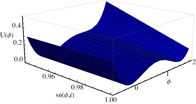
Figure 1: Plot of the effective potential when the gauge theory is taken with a small coupling. Decay of the false vacuum can occur. This effect can be seen only for $\lambda>g^{2}/4\pi$.

Gauge theory at strong coupling, such as in a confining regime, can wash the effect out. This argument is fully consistent for the Standard Model. Similarly, false-vacuum decay is also washed out when the gauge coupling gets too high values with respect to the scalar field self-coupling, as can be appreciated in Fig. 2. One can see that some values of the background field can hinder false-vacuum decay by modifying the potential significantly.

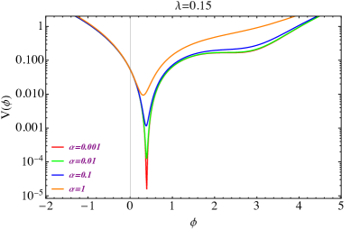
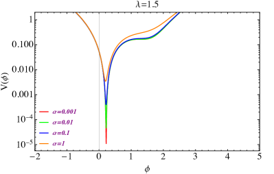
Figure 2: Plot of the effective potential having fixed $\lambda$ (coloured curves) for different values of the gauge field coupling $\alpha=g^{2}/4\pi$. Here $\theta\approx 1.06966$ and $\alpha$ varies between $0.001$ and $1$ (color bars to recognize the single curves).

Similarly, we have the plot in Fig. 3.

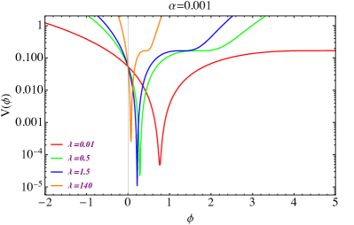
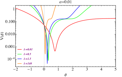
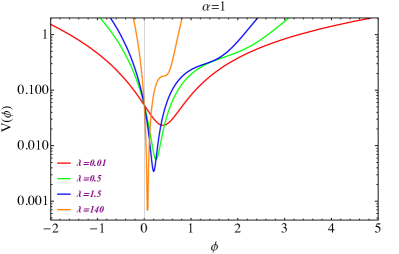
Figure 3: Plot of the effective potential having fixed values of $\alpha$ (coloured curves) for different values of the scalar field self-coupling $\lambda$. Also here $\theta\approx 1.06966$.

From Fig. 2 and 3 it is realized that increasing the gauge coupling removes the false vacuum and the decay is hindered and also non-existent. When the gauge coupling is smaller than the self-coupling of the scalar field, we get the inverse situation with the appearance of a false vacuum and a possible decay. This shows that a strongly coupled gauge field grants a stable vacuum.

In order to complete our analysis, we can evaluate the fluctuations entering into the decay rate from the standard formula Callan:1977pt

$$A=\left[\frac{\operatorname{det}^{\prime}{-\partial^{2}+V^{\prime\prime}(\phi_{0})}}{\operatorname{det}(-\partial^{2}+V^{\prime\prime}(\phi_{+}))}\right]^{-\frac{1}{2}},$$ (33)

where the prime in $\operatorname{det}^{\prime}$ means that we omit the zero mode, $\phi_{0}$ is the bounce and $\phi_{+}$ is the false vacuum. The spectrum of the operator is known: It is continuous and the eigenvalues are $3\mu^{2}\sqrt{\lambda/2}$ excluding the zero mode at $\mu=0$. Thus,

$$\operatorname{det}^{\prime}[-\partial^{2}+V^{\prime\prime}(\phi_{0})]=\prod_{\mu}\left(3\mu^{2}\sqrt{\frac{\lambda}{2}}\right)=\exp\left[\sum_{\mu}\ln\left(3\mu^{2}\sqrt{\frac{\lambda}{2}}\right)\right].$$ (34)

Let us introduce a cut-off $\Lambda$ that could be taken to be the Planck mass and promote the sum to an integral:

$$\prod_{\mu}\left(3\mu^{2}\sqrt{\frac{\lambda}{2}}\right)=\exp\left[\frac{1}{\Lambda}\int^{\Lambda}d\mu\ln\left(3\mu^{2}\frac{\lambda}{2}\right)\right]=\frac{3}{e^{2}}\sqrt{\frac{\lambda}{2}}\Lambda^{2}.$$ (35)

Similarly, we get

$$\operatorname{det}(-\partial^{2}+m^{2})=\exp\left[\frac{2}{\pi^{2}\Lambda^{4}}\int d^{4}k\ln(k^{2}+m^{2})\right]=\frac{\Lambda^{2}}{e^{\frac{1}{2}}},$$ (36)

where $m^{2}=V^{\prime\prime}(\phi_{+})$. The final result is, for $\Lambda\rightarrow\infty$,

$$A=\left(\frac{2e^{3}}{9\lambda}\right)^{\frac{1}{4}}.$$ (37)

This simple estimation, independent of the cut-off, shows that fluctuations increase as the self-coupling of the scalar field gets smaller.

IV Conclusions

The most important consequence to extract from the above results is that there is a novel interplay between the self-coupling $\lambda$ of the scalar field and the coupling $g$ of the gauge field as evident from Fig. 2 and 3. If the latter prevails, the vacuum decay is hindered and possibly impeded. When the gauge coupling is smaller than the self-coupling of the scalar field, we observe the appearance of a false vacuum and its decay decay. This shows that a strongly coupled gauge field grants a stable vacuum. This is an interesting result in view of the evolution of the universe. In fact, we can cautiously export these results to a scenario where the scalar and gauge fields live on a curved background, in which case the transition to the true vacuum is facilitated by gravity in Einstein’s theory Calcagni:2022tls . The picture that emerges is the following. At a very early stage when the temperature was higher, the scalar field coupling was higher than that of the strong interactions, possibly in a gluon-quark plasma state where the gauge coupling was very small. This configuration favoured a false-vacuum decay. When the universe cooled down, the situation became inverted and the gauge coupling dominated over the scalar one, thus preventing any further tunneling to lower vacua (which are absent in the quartic potential we considered here, but that could arise in a more complicated scenario). Therefore, the universe is very naturally driven to a stable state.

The study of false-vacuum decay with gauge theory in the presence of gravity is in our future agenda to confirm this description of the early universe.

References

- (1) B.P. Abbott et al. [LIGO Scientific and Virgo], Tests of general relativity with GW150914. Phys. Rev. Lett. 116, 221101 (2016); Erratum-Ibid. 121, 129902 (2018) [arXiv:1602.03841].
- (2) G. Degrassi, S. Di Vita, J. Elias-Miro, J.R. Espinosa, G.F. Giudice, G. Isidori and A. Strumia, Higgs mass and vacuum stability in the Standard Model at NNLO. JHEP 08, 098 (2012) [arXiv:1205.6497].
- (3) G. Isidori, G. Ridolfi and A. Strumia, On the metastability of the standard model vacuum. Nucl. Phys. B 609, 387 (2001) [arXiv:hep-ph/0104016].
- (4) P. Auclair et al. [LISA Cosmology Working Group], Cosmology with the Laser Interferometer Space Antenna. [arXiv:2204.05434].
- (5) B.P. Abbottet al.. [LIGO Scientific and VIRGO], An Upper Limit on the Stochastic Gravitational-Wave Background of Cosmological Origin. Nature 460, 990 (2009) [arXiv:0910.5772].
- (6) M. Frasca, A theorem on the Higgs sector of the Standard Model. Eur. Phys. J. Plus 131, 199 (2016) [arXiv:1504.02299].
- (7) M. Frasca, Quantum Yang–Mills field theory. Eur. Phys. J. Plus 132, 38 (2017); Erratum-ibid. 132, 242 (2017) [arXiv:1509.05292].
- (8) M. Chaichian and M. Frasca, Condition for confinement in non-Abelian gauge theories. Phys. Lett. B 781, 33-39 (2018) [arXiv:1801.09873].
- (9) M. Frasca, A. Ghoshal and S. Groote, On a novel evalutation of the hadronic contribution to the muon’s from QCD. Phys. Rev. D 104, 114036 (2021) [arXiv:2109.05041].
- (10) M. Frasca, A. Ghoshal and S. Groote, Nambu–Jona–Lasinio model correlation functions from QCD. To appear in Nucl. Part. Phys. Proc. [arXiv:2109.06465].
- (11) M. Frasca, A. Ghoshal and N. Okada, Fate of false vacuum in non-perturbative regimes. [arXiv:2201.12267].
- (12) M. Frasca, A. Ghoshal and S. Groote, Confinement in QCD and generic Yang–Mills theories with matter representations. [arXiv:2202.14023].
- (13) M. Frasca, A. Ghoshal and A. Koshelev, Quintessence dark energy from strongly-coupled Higgs mass gap: local and non-local higher-derivative non-perturbative scenarios. [arXiv:2203.15020].
- (14) G. Calcagni, M. Frasca and A. Ghoshal, Fate of false vacuum in non-perturbative regimes: Gravity effects. [arXiv:2206.09965].
- (15) A. D. Plascencia and C. Tamarit, JHEP 10 (2016), 099 doi:10.1007/JHEP10(2016)099 [arXiv:1510.07613 [hep-ph]].
- (16) M. Endo, T. Moroi, M. M. Nojiri and Y. Shoji, JHEP 11 (2017), 074 doi:10.1007/JHEP11(2017)074 [arXiv:1704.03492 [hep-ph]].
- (17) M. Endo, T. Moroi, M. M. Nojiri and Y. Shoji, Phys. Lett. B 771 (2017), 281-287 doi:10.1016/j.physletb.2017.05.057 [arXiv:1703.09304 [hep-ph]].
- (18) W. Y. Ai, J. S. Cruz, B. Garbrecht and C. Tamarit, Phys. Rev. D 102 (2020) no.8, 085001 doi:10.1103/PhysRevD.102.085001 [arXiv:2006.04886 [hep-th]].
- (19) S.R. Coleman and E.J. Weinberg, Radiative corrections as the origin of spontaneous symmetry breaking. Phys. Rev. D 7, 1888 (1973).
- (20) M. Frasca, Spectrum of Yang–Mills theory in 3 and 4 dimensions. Nucl. Part. Phys. Proc. 294-296, 124 (2018) [arXiv:1708.06184].
- (21) C.G. Callan, Jr. and S.R. Coleman, The fate of the false vacuum. 2. First quantum corrections. Phys. Rev. D 16, 1762 (1977).