Elliptically-Contoured Tensor-variate Distributions with Application to Improved Image Learning

Abstract

Statistical analysis of tensor-valued data has largely used the tensor-variate normal (TVN) distribution that may be inadequate when data comes from distributions with heavier or lighter tails. We study a general family of elliptically contoured (EC) tensor-variate distributions and derive its characterizations, moments, marginal and conditional distributions, and the EC Wishart distribution. We describe procedures for maximum likelihood estimation from data that are (1) uncorrelated draws from an EC distribution, (2) from a scale mixture of the TVN distribution, and (3) from an underlying but unknown EC distribution, where we extend Tyler’s robust estimator. A detailed simulation study highlights the benefits of choosing an EC distribution over the TVN for heavier-tailed data. We develop tensor-variate classification rules using discriminant analysis and EC errors and show that they better predict cats and dogs from images in the Animal Faces-HQ dataset than the TVN-based rules. A novel tensor-on-tensor regression and tensor-variate analysis of variance (TANOVA) framework under EC errors is also demonstrated to better characterize gender, age and ethnic origin than the usual TVN-based TANOVA in the celebrated Labeled Faces of the Wild dataset.

I Introduction

Tensor- or array-variate data arise in many disciplines, for example, in the context of relational data in political science, imaging applications in medicine or engineering, artificial intelligence and so on [1]. The tensor-variate normal (TVN) distribution [2, 3, 4, 5] is often used to model and analyze such datasets, as it generalizes the matrix-variate normal (MxVN) distribution [6, 7] to array-variate data. The TVN and MxVN distributions flow from the multivariate normal (MVN) distribution, and so benefit from the latter’s ease of interpretation, computation and inference, but also inherit its shortcomings when modeling data that arise from heavy- or light-tailed distributions.

Elliptically contoured (EC) distributions [8, 9, 10, 11, 12, 13, 14, 15] are a flexible class of symmetric vector-variate distributions that generalize the MVN distribution, and facilitate the modeling of data with heavy or light tails. In Section II we review and study properties of EC tensor-variate distributions by characterizing them, their marginal and conditional distributions and moments. We also introduce the EC tensor-variate Wishart distribution. Inference is no longer as straightforward under EC errors, so Section III provides computationally practical methodology for parameter estimation under three different scenarios, including a reduced rank tensor-on-tensor regression (ToTR) and tensor-variate analysis of variance (TANOVA) framework with EC errors, and a robust Tyler estimator for when data comes from an underlying but unknown EC distribution. We evaluate performance of our algorithms in Section IV. Section V shows the value of our methodology in two real-data scenarios. First, we develop discriminant analysis classification rules using EC tensor-variate distributions that exploit the maximum likelihood estimation frameworks developed in Section III. We use these classification rules to compare the predictive performance of the TVN and the tensor-variate-$t$ (TV-$t$) distributions in classifying cats and dogs from their images in the Animal Faces-HQ (AFHQ) database. In all cases, the flexible tensor-variate-t distribution with unknown degrees of freedom outperforms the TVN in terms of area under the receiver operating characteristic and precision-recall curves. Our second application demonstrates the ability of our ToTR and TANOVA methodology with EC errors to characterize the Labeled Faces in the Wild (LFW) dataset in terms of age, ethnic origin and gender, and compares this performance relative to that of TVN-based ToTR and TANOVA. Similarly, assuming EC errors results in preferred models according to the Bayesian information criterion. We conclude this article with a discussion on our contributions and propose further generalizations. An online supplement, with sections, theorems, equations and figures bearing the prefix “S”, provides additional technical details and supporting information as well as proofs of our theorems and lemmas.

II Definitions and Characterizations

II-A Background and preliminaries

We define a tensor as a multi-dimensional array of numbers. This article uses $\mathcal{X}$, ${\sf X}$ and $X$ to denote deterministic tensors, matrices and vectors, with bold-faced fonts for their random counterparts (e.g., $\bm{\mathcal{X}}$, $\bm{{\sf X}}$ and $\bm{X}$ denote random tensors, matrices and vectors). Further, we assume that $\mathcal{X}\in\mathbb{R}^{\times_{k=1}^{p}m_{k}}$ has $(i_{1},i_{2}\!\hbox to10.00002pt{.\hss.\hss.},i_{p})$th element written as $\mathcal{X}(i_{1},i_{2},\!\hbox to10.00002pt{.\hss.\hss.},i_{p})$. Tensor reshapings [16] allow us to modify the structure of a tensor while preserving its elements. We can reshape $\mathcal{X}$ into a $(m_{k})\times(\prod_{i=1,i\neq k}^{p}m_{i})$-matrix $\mathcal{X}_{(k)}$ using its $k$th mode matricization. The matrix $\mathcal{X}$ can also be reshaped, by means of its $k$th canonical matricization, into a $(\prod_{i=1}^{k}m_{i})\times(\prod_{i=k+1}^{p}m_{i})$ matrix $\mathcal{X}_{<k>}$, and into a vector $\operatorname{vec}(\mathcal{X})$ of $\prod_{i=1}^{p}m_{i}$ elements using vectorization – see (S2), (S3) and (S4) in Section S1-A for formal definitions.

The $k$th mode product between $\mathcal{X}$ and the $n_{k}\times m_{k}$ matrix ${\sf A}_{k}$ multiplies ${\sf A}_{k}$ to the $k$th mode of $\mathcal{X}$, resulting in the tensor $\mathcal{X}\times_{k}{\sf A}_{k}\in\mathbb{R}^{m_{1}\times\!\hbox to7.00002pt{.\hss.\hss.}\times m_{k-1}\times n_{k}\times m_{k+1}\times\!\hbox to7.00002pt{.\hss.\hss.}\times m_{p}}$. Applying the $k$th mode product with respect to ${\sf A}_{k}$ to every mode of $\mathcal{X}$ results in the Tucker (TK) product $[\![\mathcal{X};{\sf A}_{1},\!\hbox to10.00002pt{.\hss.\hss.},{\sf A}_{p}]\!]\in\mathbb{R}^{\times_{k=1}^{p}n_{k}}$ [17]. The inner product between two equal-sized tensors $\mathcal{X}$ and $\mathcal{Y}$ is defined as $(\operatorname{vec}\mathcal{X})^{\top}(\operatorname{vec}\mathcal{Y})$ and denoted as $\langle\mathcal{X},\mathcal{Y}\rangle$. If $\mathcal{B}$ is a $(p+q)$-way tensor of size $m_{1}\times m_{2}\times\ldots\times m_{p}\times h_{1}\times h_{2}\times\ldots\times h_{q}$, then the partial contraction [18] between $\mathcal{B}$ and $\mathcal{X}$ (denoted as $\langle\mathcal{X}|\mathcal{B}\rangle$) is a $q$-way tensor of size $h_{1}\times h_{2}\times\ldots\times h_{q}$ with

$$\begin{split}\langle\mathcal{X}|\mathcal{B}\rangle(j_{1},\dots,j_{q})=&\sum_{i_{1}=1}^{m_{1}}\ldots\sum_{i_{p}=1}^{m_{p}}\mathcal{X}(i_{1},\ldots,i_{p})\mathcal{B}(i_{1},\ldots,i_{p},j_{1},\ldots,j_{p}).\end{split}$$ (1)

We refer to Section S1-A for the reshaping and product definitions encountered in this section.

A random tensor $\bm{\mathcal{X}}$ is a tensor whose vectorized form $\operatorname{vec}(\bm{\mathcal{X}})$ is a random vector. In many cases $\operatorname{{\mathbb{V}}\mbox{ar}}\{\operatorname{vec}(\bm{\mathcal{X}})\}=\sigma^{2}\otimes_{k=p}^{1}\Sigma_{k}$ for $\Sigma_{k}\in\mathbb{R}^{m_{k}\times m_{k}}$, and the squared Mahalanobis distance (with respect to the scale matrices $\sigma^{2}\Sigma_{1},\!\hbox to10.00002pt{.\hss.\hss.},\Sigma_{p}$) of $\bm{\mathcal{X}}$ from its mean $\mathbb{E}(\bm{\mathcal{X}})=\mathcal{M}$ is

$$D^{2}_{\sigma^{2}\Sigma}(\bm{\mathcal{X}},\mathcal{M})=\dfrac{1}{\sigma^{2}}\langle\bm{\mathcal{X}}-\mathcal{M},[\![\bm{\mathcal{X}}-\mathcal{M};\Sigma_{1}^{-1},\!\hbox to10.00002pt{.\hss.\hss.},\Sigma_{p}^{-1}]\!]\rangle.$$ (2)

A random vector $\bm{X}$ has a vector-valued spherical distribution if its distribution is invariant to rotations: that is, for every $\Gamma\in O(h)=\{H\in\mathbb{R}^{h\times h}:HH^{\top}=I_{h}\}$, we have $\bm{X}\overset{d}{=}\Gamma\bm{X}$, or equivalently $\mathcal{L}(\bm{X})=\mathcal{L}(\Gamma\bm{X})$, with $\overset{d}{=}$ meaning distributional equality and $\mathcal{L}(\bm{X})$ meaning the law of $\bm{X}$. This notion of sphericity can be extended to a random matrix $\bm{{\sf X}}$ if it is invariant to rotations of its rows or/and columns [19]. In this article, we say that a random tensor $\bm{\mathcal{X}}\in\mathbb{R}^{\times_{k=1}^{p}m_{k}}$ follows a tensor-valued spherical distribution if $\operatorname{vec}(\bm{\mathcal{X}})$ follows a vector-valued spherical distribution. Thus $\operatorname{vec}(\bm{\mathcal{X}})\overset{d}{=}\Gamma\operatorname{vec}(\bm{\mathcal{X}})$ for any $\Gamma\in O(\prod_{k=1}^{p}h_{k})$, meaning that the distribution of $\bm{\mathcal{X}}$ is invariant under the group of transformations $\mathscr{G}=\{\varrho_{\Gamma}:\Gamma\in O(\prod_{k=1}^{p}h_{k})\}$, where $\varrho_{\Gamma}(\bm{\mathcal{X}})=\Gamma\operatorname{vec}(\bm{\mathcal{X}})$ is the matrix product of $\operatorname{vec}(\bm{\mathcal{X}})$ with the orthogonal matrix $\Gamma$. Since $\langle\bm{\mathcal{X}},\bm{\mathcal{X}}\rangle$ is maximally invariant under $\mathscr{G}$ (cf. Example 2.11 of [20]), it follows that the probability density function (PDF) $f(\cdot)$ and characteristic function (CF) $\psi(\cdot)$ are of the form

$$\psi_{\bm{\mathcal{X}}}(\mathcal{Z})=\varphi(\langle\mathcal{Z},\mathcal{Z}\rangle),\quad f_{\bm{\mathcal{X}}}(\mathcal{X})=g(\langle\mathcal{X},\mathcal{X}\rangle)$$ (3)

for some functions $\varphi$ and $g$ called the characteristic generator (CG) and probability density generator of $\bm{\mathcal{X}}$. We write $\bm{\mathcal{X}}\sim\operatorname{\mathcal{S}}_{h_{1},\!\hbox to7.00002pt{.\hss.\hss.},h_{p}}(\varphi)$ if $\bm{\mathcal{X}}$ has the CF in (3). We define EC-distributed random tensors from spherical distributions through the TK product. In the following, we will define EC distributions that are nonsingular, and have positive definite scale matrices.

Definition 1.

Suppose that $\bm{\mathcal{X}}\sim\operatorname{\mathcal{S}}_{h_{1},\!\hbox to7.00002pt{.\hss.\hss.},h_{p}}(\varphi)$, $\mathcal{M}\in\mathbb{R}^{\times_{k=1}^{p}m_{k}}$, and ${\sf Q}_{k}\in\mathbb{R}^{m_{k}\times h_{k}}$ are matrices such that ${\sf Q}_{k}{\sf Q}_{k}^{\top}=\Sigma_{k}$ is positive definite for all $k=1,\!\hbox to10.00002pt{.\hss.\hss.},p$. Then if

$$\bm{\mathcal{Y}}\overset{d}{=}\mathcal{M}+[\![\bm{\mathcal{X}};{\sf Q}_{1},\!\hbox to10.00002pt{.\hss.\hss.},{\sf Q}_{p}]\!],$$ (4)

we say that $\bm{\mathcal{Y}}$ has an EC distribution with mean $\mathcal{M}$, scale matrices $\Sigma_{1},\Sigma_{2},\!\hbox to10.00002pt{.\hss.\hss.},\Sigma_{p}$, and CG $\varphi$, written as $\bm{\mathcal{Y}}\sim\operatorname{\mathcal{E}\mathcal{C}}_{\bm{m}}(\mathcal{M},\Sigma_{1},\Sigma_{2},\!\hbox to10.00002pt{.\hss.\hss.},\Sigma_{p},\varphi),$ where $\bm{m}=(m_{1},m_{2},\!\hbox to10.00002pt{.\hss.\hss.},m_{p})^{\top}$.

For $\varphi(x)=\exp(-x/2)$, $\bm{\mathcal{Y}}$ follows the TVN distribution $\operatorname{\mathcal{N}}_{\bm{m}}(\mathcal{M},\Sigma_{1},\!\hbox to10.00002pt{.\hss.\hss.},\Sigma_{p})$. We will use $\bm{m}\!=\!(m_{1},\!\hbox to10.00002pt{.\hss.\hss.},m_{p}),m=\prod_{i=1}^{p}m_{i},m_{-k}\!=\!\frac{m}{m_{k}},\Sigma\!=\!\otimes_{i=p}^{1}\Sigma_{i},\Sigma_{-k}\!=\!\otimes_{i=p,i\neq k}^{1}\Sigma_{i}.$

Scale mixtures of TVN are an important sub-family of EC distributions, and are defined as

$$\mathcal{L}(\bm{\mathcal{Y}}|(Z=z))=\operatorname{\mathcal{N}}_{\bm{m}}(\mathcal{M},z^{-1}\Sigma_{1},\Sigma_{2},\!\hbox to10.00002pt{.\hss.\hss.},\Sigma_{p})$$ (5)

for some non-negative random variable $Z$. This distribution is the tensor-variate extension [15] of the vector-variate case studied in [21, 22, 23] and the matrix-valued case investigated in [6, 24]. A commonly-used mixing distribution in (5), for the vector-variate case, uses $Z\sim Gamma(a/2,b/2)$: doing so in the tensor-variate case yields the PDF

$$f_{\bm{\mathcal{Y}}}(\mathcal{Y})=\Big{|}\pi b\bigotimes_{k=p}^{1}\Sigma_{k}\Big{|}^{-\frac{1}{2}}\dfrac{\Gamma((m+a)/2)}{\Gamma(a/2)}\Big{(}1+\dfrac{D^{2}_{\Sigma}(\mathcal{Y},\mathcal{M})}{b}\Big{)}^{-\frac{m+a}{2}}$$ (6)

that corresponds to the TV-$t$ distribution with $\nu$ degrees of freedom (DF) when $a=b=\nu$, the tensor-variate Cauchy distribution when additionally $\nu=1$, and a tensor-variate Pearson Type VII distribution (cf. page 450 of pearson1916) with parameter $q$ when $a=m$ and $b=q$. We now derive some useful properties of the EC tensor-variate distribution.

II-B Characterizing the EC family of tensor-variate distributions

Defining EC distributions in terms of (4) allows us to extend results from the spherical family of distributions to its EC counterpart. For instance, from (3) and (4), we can write the CF of $\bm{\mathcal{Y}}$ in terms of its CG $\varphi$ as

$$\psi_{\bm{\mathcal{Y}}}(\mathcal{Z})=\exp(\imath\langle\mathcal{Z},\mathcal{M}\rangle)\varphi(\langle\mathcal{Z},[\![\mathcal{Z};\Sigma_{1},\Sigma_{2},\!\hbox to10.00002pt{.\hss.\hss.},\Sigma_{p}]\!]\rangle).$$ (7)

Similarly, if $\bm{\mathcal{X}}\sim\operatorname{\mathcal{S}}_{h_{1},h_{2},\!\hbox to7.00002pt{.\hss.\hss.},h_{p}}(\varphi)$ has the PDF in (3), then the transformation induced in (4) has Jacobian determinant $|\bigotimes_{k=p}^{1}\Sigma_{k}|^{-1/2}$, so the PDF of $\bm{\mathcal{Y}}$ is

$$f_{\bm{\mathcal{Y}}}(\mathcal{Y})=\Big{|}\bigotimes_{k=p}^{1}\Sigma_{k}\Big{|}^{-1/2}g(D^{2}_{\Sigma}(\mathcal{Y},\mathcal{M})),$$ (8)

where $D^{2}(\cdot)$ is the squared Mahalanobis distance of (2). Table I

TABLE I: Some common EC distributions, defined using (8) with their corresponding probability density generators $g(\dot{)}$, given upto their constant of proportionality.

Distribution	Additional	$g(x)$
	parameters
Normal	–	$\exp(-x/2)$
Student’s-$t$	$q>0$	$(1+q^{-1}x)^{-(q+m)/2}$
Pearson Type VII	$q>0$	$(1+x/q)^{-m}$
Kotz Type	$q>0$	$x^{m-1}\exp(-qx)$
Logistic	–	$\exp(-x)/(1+\exp(-x))^{2}$
Power exponential	$q>0$	$\exp(-x^{q}/2)$

defines some EC distributions by specifying the density generator function $g(\cdot)$ (for additional specifications, see [25, 26]).

The following theorem allows us to express EC tensor-variate distributions in terms of vector-variate EC distributions that have been studied extensively in the literature.

Theorem 2.

With the reshapings of (S2), (S3) and (S4), and for all $k=1,2,\!\hbox to10.00002pt{.\hss.\hss.},p$, the following statements are equivalent, with $n_{k}=\prod_{i=1}^{k}m_{i}$:

1. $\bm{\mathcal{Y}}\sim\operatorname{\mathcal{E}\mathcal{C}}_{\bm{m}}(\mathcal{M},\Sigma_{1},\Sigma_{2},\!\hbox to10.00002pt{.\hss.\hss.},\Sigma_{p},\varphi)$.

2. $\bm{\mathcal{Y}}_{(k)}\sim\operatorname{\mathcal{E}\mathcal{C}}_{m_{k},m_{-k}}(\mathcal{M}_{(k)},\Sigma_{k},\Sigma_{-k},\varphi)$

3. $\bm{\mathcal{Y}}_{<k>}\sim\operatorname{\mathcal{E}\mathcal{C}}_{n_{k},m/n_{k}}(\mathcal{M}_{<k>},\bigotimes_{i=k}^{1}\Sigma_{i},\bigotimes_{i=p}^{k+1}\Sigma_{i},\varphi)$.

4. $\operatorname{vec}(\bm{\mathcal{Y}})\sim\operatorname{\mathcal{E}\mathcal{C}}_{m}(\operatorname{vec}(\mathcal{M}),\Sigma,\varphi)$.

Proof.

See the Supplementary Material Section S3-A. ∎

Spherical distributions receive their name from the observation that if $\bm{\mathcal{X}}\sim\operatorname{\mathcal{S}}_{h_{1},h_{2},\ldots,h_{p}}(\varphi)$, then $\bm{\mathcal{X}}=R\bm{\mathcal{U}},$ where the magnitude $R=||\bm{\mathcal{X}}||$ is independent from $\bm{\mathcal{U}}$ and $\operatorname{vec}(\bm{\mathcal{U}})$ is uniformly distributed in the shell of a unit sphere of dimension $\prod_{k=1}^{p}h_{k}$ [27, 8, 28]. Based on the CF in (3) and the independence of $R$ and $\bm{\mathcal{U}}$ , we have that $\psi_{\bm{\mathcal{X}}}(\mathcal{Z})=\mathbb{E}\{\psi_{\bm{\mathcal{U}}}(R\mathcal{Z})\},$ and since $\bm{\mathcal{U}}$ is also spherically distributed, the CG of $\bm{\mathcal{X}}$ can be written, in terms of the CG of $\bm{\mathcal{U}}$, as

$$\varphi(u)=\mathbb{E}\{\varphi_{\bm{\mathcal{U}}}(R^{2}u)\}.$$ (9)

The distribution of $R$ determines the distribution of $\bm{\mathcal{X}}$. For instance, if $R^{2}\sim\chi^{2}_{h}$, where $h=\prod_{k=1}^{p}h_{k}$, then $\varphi(u)=\exp(-u/2)$ and $\bm{\mathcal{X}}$ follows a TVN distribution. Further, if $\bm{\mathcal{Y}}\sim\operatorname{\mathcal{E}\mathcal{C}}_{\bm{m}}(0,\sigma^{2}\Sigma_{1},\!\hbox to10.00002pt{.\hss.\hss.},\Sigma_{p},\varphi)$ as in equation (4) and $\bm{\mathcal{X}}=R\bm{\mathcal{U}}$ as above, then $\bm{\mathcal{Z}}=\bm{\mathcal{Y}}/||\bm{\mathcal{Y}}||$ does not depend on $R$, meaning that the distribution of $\bm{\mathcal{Z}}$ does not depend on the original EC distribution of $\bm{\mathcal{Y}}$. The distribution of $\bm{Z}=\operatorname{vec}(\bm{\mathcal{Z}})$ is called the elliptical angular distribution [29, 30], and is denoted as $\bm{Z}\sim\operatorname{\mathcal{A}\mathcal{C}}_{m}(\Sigma)$, with PDF

$$f_{\bm{Z}}(\bm{z})=\frac{\Gamma(m/2)}{2\pi^{m/2}}|\Sigma|^{-1/2}(\bm{z}^{\top}\Sigma^{-1}\bm{z})^{-m/2}.$$ (10)

The above PDF does not depend on $\sigma^{2}$. In Section III-E, we derive a robust tensor-variate Tyler estimator that exploits the fact that $\bm{\mathcal{Z}}$ is the same for any EC distribution.

II-C Marginal and conditional distributions

Our next theorem shows that the TK product of an EC distributed random tensor is also EC distributed.

Theorem 3.

Let $\bm{\mathcal{Y}}\!\sim\!\operatorname{\mathcal{E}\mathcal{C}}_{\bm{m}}(\mathcal{M},\Sigma_{1},\!\hbox to10.00002pt{.\hss.\hss.},\Sigma_{p},\varphi)$ and ${\sf A}_{k}\in\mathbb{R}^{n_{k}\times m_{k}}$ $\forall k=1,\!\hbox to10.00002pt{.\hss.\hss.},p$. Then

$$\begin{split}[\![\bm{\mathcal{Y}};{\sf A}_{1},\!\hbox to10.00002pt{.\hss.\hss.},{\sf A}_{p}]\!]\sim\operatorname{\mathcal{E}\mathcal{C}}_{[n_{1},\!\hbox to7.00002pt{.\hss.\hss.},n_{p}]}&([\![\mathcal{M};{\sf A}_{1},\!\hbox to10.00002pt{.\hss.\hss.},{\sf A}_{p}]\!],{\sf A}_{1}\Sigma_{1}{\sf A}_{1}^{\top},\!\hbox to10.00002pt{.\hss.\hss.},{\sf A}_{p}\Sigma_{p}{\sf A}_{p}^{\top},\varphi).\end{split}$$

Proof.

See the Supplementary Material Section S3-B. ∎

As a corollary, the marginal distributions follow from Theorem 3 by choosing ${\sf A}_{1},\!\hbox to10.00002pt{.\hss.\hss.},{\sf A}_{p}$ appropriately, as described in detail in Section S1-B. We now extend the vector-variate result of [27] to derive conditional distributions in the tensor-variate setting.

Theorem 4.

Suppose that $\bm{\mathcal{Y}}\sim\operatorname{\mathcal{E}\mathcal{C}}_{\bm{m}}(\mathcal{M},\Sigma_{1},\!\hbox to10.00002pt{.\hss.\hss.},\Sigma_{p},\varphi)$, where $m_{p}=n_{1}+n_{2}>1$ for some $n_{1},n_{2}\in\mathbb{N}$, and $\Sigma_{p}$ is a block matrix with $(i,j)$th block $\Sigma_{ij}\in\mathbb{R}^{n_{i}\times n_{j}}$. Partition $\bm{\mathcal{Y}}$ and $\mathcal{M}$ over the $pth$ mode with $\bm{\mathcal{Y}}_{1},\mathcal{M}_{1}\in\mathbb{R}^{m_{1}\times m_{2}\times\ldots\times m_{p-1}\times n_{1}}$ and $\bm{\mathcal{Y}}_{2},\mathcal{M}_{2}\in\mathbb{R}^{m_{1}\times m_{2}\times\ldots\times m_{p-1}\times n_{2}}$. Then

$$\begin{split}\bm{\mathcal{Y}}_{1}|(\bm{\mathcal{Y}}_{2}=\mathcal{Y}_{2})\sim\operatorname{\mathcal{E}\mathcal{C}}_{[m_{1},\!\hbox to7.00002pt{.\hss.\hss.},m_{p-1},n_{1}]}\Big{(}\mathcal{M}_{\{1\}|\{2\}},\Sigma_{1},\!\hbox to10.00002pt{.\hss.\hss.},\Sigma_{p-1},\Sigma_{p,\{11\}|\bullet},\varphi_{q(\mathcal{Y}_{2})}\Big{)},\end{split}$$ (11)

where $\mathcal{M}_{\{1\}|\{2\}}=\mathcal{M}_{1}+(\mathcal{Y}_{2}-\mathcal{M}_{2})\times_{p}(\Sigma_{p,12}\Sigma_{p,22}^{-1})$ , $\Sigma_{p,\{11\}|\bullet}=\Sigma_{p,11}-\Sigma_{p,12}\Sigma_{p,22}^{-1}\Sigma_{p,21}$ , $\varphi_{q(\mathcal{Y}_{2})}(u)=\mathbb{E}\{R^{2}_{q(\bm{\mathcal{Y}}_{2})}\varphi_{\bm{\mathcal{U}}}(u)|\bm{\mathcal{Y}}_{2}=\mathcal{Y}_{2}\}$, $R^{2}_{q(\bm{\mathcal{Y}}_{2})}\!=\!D^{2}_{\Sigma_{\bullet}}(\bm{\mathcal{Y}}_{1},\mathcal{M}_{1}),$ and $\Sigma_{\bullet}\!=\!\Sigma_{p,\{11\}|\bullet}\otimes\Sigma_{-1}.$

Proof.

See the Supplementary Material Section S3-C. ∎

The CG $\varphi_{q}(\mathcal{Y}_{2})$ in (11) is a conditional moment, just like in the more general case of (9). Although Theorem 4 applies only for the conditional distribution that results from partitioning the last mode of the random tensor, we can find conditional distributions of any subtensor by applying Theorem 4 multiple times, as demonstrated in Section S1-C.

II-D Moments

The moments of EC tensor-variate distributions are found by differentiating (7). We provide the first four moments in Theorem 5 and then use them in Theorem 6 to find moments of other special forms.

Theorem 5.

Suppose $\bm{\mathcal{Y}}\sim\operatorname{\mathcal{E}\mathcal{C}}_{\bm{m}}(\mathcal{M},\Sigma_{1},\Sigma_{2},\!\hbox to10.00002pt{.\hss.\hss.},\Sigma_{p},\varphi)$, and let $\bm{i}=(i_{1},\!\hbox to10.00002pt{.\hss.\hss.},i_{p})^{\top}$, $\bm{j}=(j_{1},\!\hbox to10.00002pt{.\hss.\hss.},j_{p})^{\top}$, $\bm{k}=(k_{1},\!\hbox to10.00002pt{.\hss.\hss.},k_{p})^{\top}$ and $\bm{l}=(l_{1},\!\hbox to10.00002pt{.\hss.\hss.},l_{p})^{\top}$ be sets of indices such that $i_{q},j_{q},k_{q},l_{q}\in\{1,\!\hbox to10.00002pt{.\hss.\hss.},m_{q}\}$ for $q=1,\!\hbox to10.00002pt{.\hss.\hss.},p$. Further, denote $\bm{\mathcal{Y}}(i_{1},\!\hbox to10.00002pt{.\hss.\hss.},i_{p})=Y_{\bm{i}}$, $\mathcal{M}(i_{1},\!\hbox to10.00002pt{.\hss.\hss.},i_{p})=m_{\bm{i}}$ and $\sigma_{\bm{i}\bm{j}}=\prod_{q=1}^{p}\Sigma_{q}(i_{q},j_{q})$. Then

1. $\mathbb{E}(Y_{\bm{i}})=m_{\bm{i}}$.

2. $\mathbb{E}(Y_{\bm{i}}Y_{\bm{j}})=m_{\bm{i}}m_{\bm{j}}-2\varphi^{\prime}(0)\sigma_{\bm{i}\bm{j}}$.

3. $\mathbb{E}(Y_{\bm{i}}Y_{\bm{j}}Y_{\bm{k}})=m_{\bm{i}}m_{\bm{j}}m_{\bm{k}}-2\varphi^{\prime}(0)(m_{\bm{i}}\sigma_{\bm{k}\bm{j}}+m_{\bm{j}}\sigma_{\bm{i}\bm{k}}+m_{\bm{k}}\sigma_{\bm{i}\bm{j}}).$

4. $\mathbb{E}(Y_{\bm{i}}Y_{\bm{j}}Y_{\bm{k}}Y_{\bm{l}})=m_{\bm{i}}m_{\bm{j}}m_{\bm{k}}m_{\bm{l}}+4\varphi^{\prime\prime}(0)\Big{(}\sigma_{\bm{k}\bm{l}}\sigma_{\bm{j}\bm{i}}+\sigma_{\bm{j}\bm{l}}\sigma_{\bm{i}\bm{k}}+\sigma_{\bm{i}\bm{l}}\sigma_{\bm{j}\bm{k}}\Big{)}-2\varphi^{\prime}(0)\Big{(}m_{\bm{l}}m_{\bm{k}}\sigma_{\bm{i}\bm{j}}+m_{\bm{j}}m_{\bm{l}}\sigma_{\bm{i}\bm{k}}+m_{\bm{j}}m_{\bm{k}}\sigma_{\bm{i}\bm{l}}+m_{\bm{i}}m_{\bm{l}}\sigma_{\bm{j}\bm{k}}+m_{\bm{i}}m_{\bm{k}}\sigma_{\bm{j}\bm{l}}+m_{\bm{i}}m_{\bm{j}}\sigma_{\bm{k}\bm{l}}\Big{)}.$

Here, the $k$th statement of the theorem requires $\varphi^{(k)}(0)<\infty$, for $k=1,2,3,4$.

Proof.

See the Supplementary Material Section S3-D. ∎

Theorem 3 allows us to derive many different moments. We derive some of them now.

Theorem 6.

Let $\bm{\mathcal{Y}}\sim\operatorname{\mathcal{E}\mathcal{C}}_{\bm{m}}(\mathcal{M},\Sigma_{1},\Sigma_{2},\ldots,\Sigma_{p},\varphi)$, where $\varphi^{\prime\prime}(0)\!<\!\infty$. Further, let ${\sf A}_{k}$ and ${\sf B}_{k}$ be $n_{k}\times m_{k}$ and $h_{k}\times m_{k}$ matrices for $k=1,2,\ldots,p$, and define $D^{2}_{A}(\mathcal{X})=\langle\mathcal{X},[\![\mathcal{X};{\sf A}_{1},{\sf A}_{2},\!\hbox to10.00002pt{.\hss.\hss.},{\sf A}_{p}]\!]\rangle$ whenever each $A_{k}$ is a square matrix. Then,

1. $\mathbb{E}(\bm{\mathcal{Y}})=\mathcal{M}$.

2. $\operatorname{{\mathbb{V}}\mbox{ar}}\{\operatorname{vec}(\bm{\mathcal{Y}})\}=-2\varphi^{\prime}(0)\bigotimes\limits_{k=p}^{1}\Sigma_{k}.$

3. If $n_{k}=m_{k}$ for all $k=1,2,\ldots,p$, then

   $\mathbb{E}\left\{D^{2}_{A}(\bm{\mathcal{Y}})\right\}=D^{2}_{A}(\mathcal{M})-2\varphi^{\prime}(0)\prod\limits_{k=1}^{p}\operatorname{tr}(\Sigma_{k}{\sf A}_{k}^{\top}).$

4. If $\mathcal{V}$ is of size $n_{1}\times n_{2}\times\ldots\times n_{p}$, then

   $\mathbb{E}(\langle\mathcal{V},[\![\bm{\mathcal{Y}};{\sf A}_{1},\ldots,{\sf A}_{p}]\!]\rangle\bm{\mathcal{Y}})=\langle\mathcal{V},[\![\mathcal{M};{\sf A}_{1},\ldots,{\sf A}_{p}]\!]\rangle\mathcal{M}-2\varphi^{\prime}(0)[\![\mathcal{V};\Sigma_{1}{\sf A}_{1}^{\top},\ldots,\Sigma_{p}{\sf A}_{p}^{\top}]\!].$

5. If $n_{k}=m_{k}$ for all $k=1,2,\ldots,p$, then

   $-2\varphi^{\prime}(0)\Big{[}\prod\limits_{k=1}^{p}\operatorname{tr}(\Sigma_{k}{\sf A}_{k}^{\top})\mathcal{M}+[\![\mathcal{M};\Sigma_{1}{\sf A}_{1},\ldots,\Sigma_{p}{\sf A}_{p}]\!]+[\![\mathcal{M};\Sigma_{1}{\sf A}_{1}^{\top},\ldots,\Sigma_{p}\sf A_{p}^{\top}]\!]\Big{]}.$

6. If $\mathcal{M}=0$, $\varphi^{(4)}(0)<\infty$ and $n_{k}=h_{k}=m_{k}$ for all $k=1,\ldots,p$, then

   $\mathbb{E}\big{\{}D^{2}_{A}(\bm{\mathcal{Y}})D^{2}_{B}(\bm{\mathcal{Y}})\big{\}}\!=\!4\varphi^{\prime\prime}(0)\Big{[}\prod\limits_{k=1}^{p}\left\{\operatorname{tr}({\sf A}_{k}\Sigma_{k})\operatorname{tr}({\sf B}_{k}\Sigma_{k})\right\}+\prod\limits_{k=1}^{p}\operatorname{tr}({\sf A}_{k}\Sigma_{k}{\sf B}_{k}^{\top}\Sigma_{k})\!+\!\prod\limits_{k=1}^{p}\operatorname{tr}({\sf A}_{k}\Sigma_{k}{\sf B}_{k}\Sigma_{k})\Big{]}.$

Proof.

See the Supplementary Material Section S3-E. ∎

From Parts 3 and 6 of Theorem 6, we see that for $\bm{\mathcal{Y}}$ specified as in Definition 1, $\mathbb{E}\{D^{2}_{\Sigma}(\bm{\mathcal{Y}},\mathcal{M})\}=-2\varphi^{\prime}(0)\times m$, and $\mathbb{V}ar\{D^{2}_{\Sigma}(\bm{\mathcal{Y}},\mathcal{M})\}=4\times[\varphi^{\prime\prime}(0)\times(m^{2}+2m)-(\varphi^{\prime}(0)\times m)^{2}].$

II-E The EC tensor-variate Wishart distribution

The Wishart distribution [31] plays an important role in multivariate statistics in inference on sample dispersion matrices [32]. The matrix-variate EC Wishart distribution was proposed in [33, 34, 35] as per

Definition 7.

A matrix $\bm{{\sf S}}$ is said to follow an EC matrix-variate Wishart distribution with DF $n$, scale parameter $\Sigma$ and CG $\varphi$, written as $\bm{{\sf S}}\sim\operatorname{\mathcal{E}\mathcal{C}\mathcal{W}}_{m}(n,\Sigma,\varphi)$, if there exists a random matrix $\bm{{\sf X}}\sim\operatorname{\mathcal{E}\mathcal{C}}_{m,n}(0,\Sigma,I_{n},\varphi)$ such that $\bm{{\sf S}}\overset{d}{=}\bm{{\sf X}}\bm{{\sf X}}^{\top}$.

If $n>m$, then the PDF of $\bm{{\sf S}}$ can be written as

$$f_{\bm{{\sf S}}}({\sf S})=\dfrac{\pi^{mn/2}}{\Gamma_{m}(n/2)|\Sigma|^{n/2}}|{\sf S}|^{(n-m-1)/2}g(\operatorname{tr}(\Sigma^{-1}{\sf S})),$$ (12)

where $g(\cdot)$ is the density generator of $\bm{{\sf X}}$. For $n<m$, we have the singular matrix-variate EC Wishart distribution. For completeness, we derive the PDF of the functionally independent elements of $\bm{{\sf S}}$ when $n<m$ in Section S1-D. We now define the EC TV Wishart distribution.

Definition 8.

The random tensor $\bm{\mathcal{S}}\in\mathbb{R}^{\times_{j=1}^{p}m_{j}}$ follows a tensor-valued EC Wishart distribution with DF $n$, scale matrices $\Sigma_{1},\Sigma_{2},\!\hbox to10.00002pt{.\hss.\hss.},\Sigma_{p}$ and CG $\varphi$ (i.e., $\bm{\mathcal{S}}\sim\operatorname{\mathcal{E}\mathcal{C}\mathcal{W}}_{\bm{m}}(n,\Sigma_{1},\!\hbox to10.00002pt{.\hss.\hss.},\newline \Sigma_{p},\varphi)$) if $\bm{\mathcal{S}}_{<p>}\sim\operatorname{\mathcal{E}\mathcal{C}\mathcal{W}}_{m}(n,\Sigma,\varphi)$.

In the vector-variate case, the Wishart distribution can be constructed from the vector outer product sum of independent and identically distributed (IID) MVN-distributed random vectors. Similarly, the EC tensor-variate Wishart distribution can be constructed from the outer tensor product sum of uncorrelated tensors $\bm{\mathcal{Y}}_{1},\bm{\mathcal{Y}}_{2},\!\hbox to10.00002pt{.\hss.\hss.},\bm{\mathcal{Y}}_{n}$ (where $\bm{\mathcal{Y}}_{i}=\bm{\mathcal{Y}}\times_{p+1}{\bm{e}_{i}^{n}}^{\top}$ for all $i=1,2,\dots,n$ and $\bm{e}_{i}^{n}\in\mathbb{R}^{n}$ is a unit basis vector with 1 as the $i$th element and 0 elsewhere) which jointly follow

$$\bm{\mathcal{Y}}\sim\operatorname{\mathcal{E}\mathcal{C}}_{[\bm{m},n]^{\top}}(\mathcal{M}_{n},\sigma^{2}\Sigma_{1},\Sigma_{2},\!\hbox to10.00002pt{.\hss.\hss.},\Sigma_{p},I_{n},\varphi).$$ (13)

Here $\Sigma_{k}$ is constrained to have $\Sigma_{k}(1,1)=1$ for all $k=1,2,\dots,p$ while $\sigma^{2}$ captures the overall proportionality constraint of $\Sigma$, and $\mathcal{M}_{n}\times_{p+1}{\bm{e}_{i}^{n}}^{\top}=\mathcal{M}$ for all $i=1,2,\!\hbox to10.00002pt{.\hss.\hss.},n$. In the next theorem, we show that $\bm{\mathcal{Y}}_{1},\bm{\mathcal{Y}}_{2},\!\hbox to10.00002pt{.\hss.\hss.}\bm{\mathcal{Y}}_{n}$ are uncorrelated, have identical marginal distributions, and that their tensor outer product sum follows the EC Wishart distribution.

Theorem 9.

Let $\bm{\mathcal{Y}}_{1},\bm{\mathcal{Y}}_{2}\ldots,\bm{\mathcal{Y}}_{n}$ jointly follow the distribution in (13). Then, we have:

1. $\bm{\mathcal{Y}}_{i}\sim\operatorname{\mathcal{E}\mathcal{C}}_{\bm{m}}(\mathcal{M},\sigma^{2}\Sigma_{1},\Sigma_{2},\!\hbox to10.00002pt{.\hss.\hss.},\Sigma_{p},\varphi)$ and $\forall i\neq j,\mathbb{E}\left(\operatorname{vec}(\bm{\mathcal{Y}}_{i}-\mathcal{M})\operatorname{vec}(\bm{\mathcal{Y}}_{j}-\mathcal{M})^{\top}\right)=0$.

2. $\sum\limits_{i=1}^{n}(\bm{\mathcal{Y}}_{i}\circ\bm{\mathcal{Y}}_{i})\sim\operatorname{\mathcal{E}\mathcal{C}\mathcal{W}}_{\bm{m}}(n,\sigma^{2}\Sigma_{1},\Sigma_{2},\!\hbox to10.00002pt{.\hss.\hss.},\Sigma_{p},\varphi).$

Here $\circ$ denotes the tensor outer product that we define in Section S1-A.

Proof.

See the Supplementary Material Section S3-F. ∎

In Section III-B we derive maximum likelihood estimators (MLEs) estimators for $(\mathcal{M},\sigma^{2},\newline \Sigma_{1},\Sigma_{2},\!\hbox to10.00002pt{.\hss.\hss.},\Sigma_{p})$ under the assumption that $\bm{\mathcal{Y}}_{1},\bm{\mathcal{Y}}_{2},\!\hbox to10.00002pt{.\hss.\hss.},\bm{\mathcal{Y}}_{n}$ are uncorrelated, as implied in (13), which is a generalization of the traditional IID assumption. Setting $\varphi(z)=\exp(-z/2)$ leads to the case where IID $\bm{\mathcal{Y}}_{i}\sim\operatorname{\mathcal{N}}_{\bm{m}}(0,\sigma^{2}\Sigma_{1},\Sigma_{2},\!\hbox to10.00002pt{.\hss.\hss.},\Sigma_{p})$ results in $\sum_{i=1}^{n}(\bm{\mathcal{Y}}_{i}\circ\bm{\mathcal{Y}}_{i})\sim\mathcal{W}_{\bm{m}}(n,\sigma^{2}\Sigma_{1},\Sigma_{2},\!\hbox to10.00002pt{.\hss.\hss.},\Sigma_{p})$.

III Maximum likelihood estimation

This section derives MLEs from EC tensor-variate distributed data under four different scenarios. We first derive these estimators from uncorrelated draws that have common and joint EC tensor-variate distributions. This procedure depends on identifiable MLEs from the TVN distribution, and so we also describe how to obtain such estimates. Next, we provide expectation conditional maximization (ECM) [36, 37] and ECM Either (ECME) [38] algorithms for maximum likelihood estimation on IID realizations from a scale TVN mixture distribution, and show how these estimation algorithms can be used to extend the ToTR framework of [18] to the case where the error distribution is a scale mixture of TVNs. Finally, we derive a robust estimation algorithm for the scale matrices in the spirit of Tyler’s estimation [39, 40, 41] for unknown EC distributions.

III-A Estimation in the TVN model

Suppose that we independently observe $\mathcal{Y}_{1},\mathcal{Y}_{2},\dots,\mathcal{Y}_{n}$ from $\operatorname{\mathcal{N}}_{\bm{m}}(0,\sigma^{2}\Sigma_{1},\Sigma_{2},\dots,\Sigma_{p})$. The MLEs of the scale matrices $\Sigma_{1},\Sigma_{2},\dots,\Sigma_{p}$ are not identifiable since $\Sigma_{k}\otimes\Sigma_{l}=(a\Sigma_{k})\otimes(\Sigma_{l}/a)$ for any scalar $a\neq 0$. Moreover, the scale matrix estimators have no closed-form solutions, but each $\widehat{\Sigma}_{k}$ depends on the rest as $\widehat{\Sigma}_{k}={\sf S}_{k}/(nm_{-k}\sigma^{2})$, where ${\sf S}_{k}=\sum_{i=1}^{n}\mathcal{Y}_{i(k)}\Sigma_{-k}^{-1}\mathcal{Y}_{i(k)}^{\prime},$ with $\Sigma_{-k}$ as defined in the paragraph following Definition 1. The existing methodology [42, 43, 44, 45, 46] takes into account the indeterminacy of the estimates by scaling each $\widehat{\Sigma}_{k}$ such that the trace, determinant or $(1,1)$th element is unity. Alternatively, we use the ADJUST procedure of [47] that optimizes the loglikelihood with respect to $\Sigma_{k}$ under the constraint $\Sigma_{k}(1,1)=1$ as $\widehat{\Sigma}_{k}=ADJUST(nm_{-k},\sigma^{2},{\sf S}_{k}).$ Here $\sigma^{2}$ is inexpensively estimated to be $\widehat{\sigma}^{2}=\operatorname{tr}(S_{k}\widehat{\Sigma}_{k}^{-1})/(nm)$. These form our minor modifications to the maximum likelihood estimation algorithm of [2, 3, 4, 5], but will be used in the following section.

III-B Estimation from uncorrelated data with identical EC-distributed marginal distributions

Suppose that we observe realizations $\mathcal{Y}_{1},\mathcal{Y}_{2},\!\hbox to10.00002pt{.\hss.\hss.},\mathcal{Y}_{n}$ of random tensors that have the same setting as Theorem 9. Our derivation of MLEs under the joint EC distributional assumption of (13) is then a tensor-variate extension of Theorem 1 of [48], and is as follows:

Theorem 10.

Suppose that the density generator $g(\cdot)$ of $\bm{\mathcal{Y}}$ is such that $h(d)=d^{nm/2}g(d)$ has a finite positive maximum $d_{g}$. Also, let $(\widetilde{\sigma}^{2},\widetilde{\mathcal{M}},\widetilde{\Sigma}_{1},\widetilde{\Sigma}_{2},\dots,\widetilde{\Sigma}_{p})$ be the TVN MLEs described in Section III-A. Then the MLE for $(\sigma^{2},\mathcal{M},\Sigma_{1},\Sigma_{2},\dots,\Sigma_{p})$ is
$(\frac{nm}{d_{g}}\widetilde{\sigma}^{2},\widetilde{\mathcal{M}},\widetilde{\Sigma}_{1},\widetilde{\Sigma}_{2},\dots,\widetilde{\Sigma}_{p})$.

Proof.

See the Supplementary Material Section S3-G. ∎

It follows that $d_{g}=mn$ in the TVN case, $d_{g}=nmb/a$ when $g(\cdot)$ is of the form (6), $d_{g}=(mn/s)^{1/s}$ in the power exponential case, and $d_{g}$ is the solution to $mn/(2d)=\tanh\left(d/2\right)$ in the logistic case [26, 13].

III-C Estimation from TVN scale mixture realizations

Suppose that we observe $n$ IID realizations $\mathcal{Y}_{1},\mathcal{Y}_{2},\dots,\mathcal{Y}_{n}$ from the scale mixture distribution of (5). The complete-data loglikelihood is

$$\ell_{c}(\bm{\theta})=-\dfrac{n}{2}\log|\sigma^{2}\Sigma|-\dfrac{1}{2\sigma^{2}}\sum_{i=1}^{n}z_{i}D^{2}_{\Sigma}(\mathcal{Y}_{i},\mathcal{M})$$ (14)

where $\bm{\theta}=\left((\operatorname{vec}\mathcal{M})^{\top},\bm{\theta}_{\Sigma}^{\top}\right)^{\top}$, and $\bm{\theta}_{\Sigma}=\big{(}\sigma^{2},(\operatorname{vec}\Sigma_{1})^{\top},(\operatorname{vec}\Sigma_{2})^{\top}\dots,$ $(\operatorname{vec}\Sigma_{p})^{\top}\big{)}^{\top}.$ We now use $\ell_{c}$ to propose an EM algorithm with the following expectation (E) and conditional maximization (CM) steps:
E-step: Here, we obtain the conditional expectation of (14), given the observed data and evaluated at the $t$th parameter iteration $\bm{\theta}^{(t)}$, to get

$$Q(\bm{\theta};\bm{\theta}^{(t)})=-\dfrac{n}{2}\log|\sigma^{2}\Sigma|-\dfrac{1}{2\sigma^{2}}\sum_{i=1}^{n}\widehat{z}_{i}^{(t)}D^{2}_{\Sigma}(\mathcal{Y}_{i},\mathcal{M}),$$ (15)

where $\widehat{z}_{i}^{(t)}=\mathbb{E}(Z_{i}|\bm{\mathcal{Y}}_{i}=\mathcal{Y}_{i};\bm{\theta}^{(t)}).$ This conditional expectation depends on the distribution of $Z_{i}$. For $Z_{i}\sim Gamma(a/2,b/2)$, $\bm{\mathcal{Y}}_{i}$ has PDF given by (6) and then $\widehat{z}_{i}^{(t)}={(m+a)}/(D^{2}_{\sigma^{2(t)}\Sigma^{(t)}}(\mathcal{Y}_{i},\mathcal{M}^{(t)})+b).$
CM-steps: The CM steps maximize (15), but with respect to subsets of parameters. The first CM step maximizes (15) with respect to $\mathcal{M}$ and is obtained by setting to zero the total differential on $\mathcal{M}$, that is, $\partial Q(\mathcal{M})=(\sigma^{2})^{-1}\langle\partial\mathcal{M},[\![\mathcal{S};\Sigma_{1}^{-1},\Sigma_{2}^{-1},\dots,\Sigma_{p}^{-1}]\!]\rangle=0,$ where $\mathcal{S}=\sum_{i=1}^{n}\widehat{z}_{i}^{(t)}\mathcal{Y}_{i}-\mathcal{M}\sum_{i=1}^{n}\widehat{z}_{i}^{(t)}.$ The term $\partial Q(\mathcal{M})=0$ implies that $\mathcal{S}=0$, or $\mathcal{\widehat{M}}^{(t+1)}=(\sum_{i=1}^{n}\widehat{z}_{i}^{(t)}\mathcal{Y}_{i})/(\sum_{i=1}^{n}\widehat{z}_{i}^{(t)}).$ Setting $\mathcal{M}=\mathcal{\widehat{M}}^{(t+1)}$ in (15) profiles out $\mathcal{M}$ and again yields (15), but with $\mathcal{Y}_{w,i}^{(t)}=\sqrt{\widehat{z}_{i}}^{(t)}(\mathcal{Y}_{i}-\mathcal{\widehat{M}}^{(t+1)})$ instead of $\mathcal{Y}_{i}$. This profiled loglikelihood is identical to the loglikelihood of the TVN model when $\mathcal{Y}_{w,i}^{(t)}\sim\operatorname{\mathcal{N}}_{\bm{m}}(0,\sigma^{2}\Sigma_{1},\Sigma_{2},\dots,\Sigma_{p})$, and thus the next $(p+1)$ CM steps (corresponding to $\sigma^{2},\Sigma_{1},\Sigma_{2},\dots,\Sigma_{p}$) are obtained similarly as for the TVN model of Section III-A. Specifically, $\widehat{\Sigma}_{k}=ADJUST(nm_{-k},\sigma^{2},{\sf S}_{k}),$ and $\sigma^{2}=\operatorname{tr}(S_{k}\widehat{\Sigma}_{k}^{-1})/(nm)$.
EM algorithm: The ECM algorithm iterates the E- and CM-steps until convergence. We determine convergence based on the relative difference in $||\mathcal{M}||+||\sigma^{2}\Sigma||,$ where $||\sigma^{2}\Sigma||=\sigma^{2}\prod_{k=1}^{p}||\Sigma_{k}||$. The resulting ECM algorithm is summarized in the following steps:

1. Initialization: Fit the faster TVN model of Section III-A with lax convergence, set $t=0$.

2. E-Step: Find $\widehat{z}_{i}^{(t)}:=\mathbb{E}(Z_{i}|\bm{\mathcal{Y}}_{i}=\mathcal{Y}_{i};\bm{\theta}^{(t)})$ $\forall i=1,2,\dots,n$.

3. CM-Step 1: Find $\mathcal{\widehat{M}}^{(t+1)}=(\sum_{i=1}^{n}\widehat{z}_{i}^{(t)}\mathcal{Y}_{i})/(\sum_{i=1}^{n}\widehat{z}_{i}^{(t)}).$

4. CM-Step 2: For each $k=1,2,\dots p$, estimate $\widehat{\Sigma}_{k}$.

5. CM-Step 3: estimate $\sigma^{2}$.

6. Iterate or stop: Return to the E-step and set $t\leftarrow t+1$, or stop if convergence is met.

Alternative EM approach for estimating $\bm{\sigma^{2}}$: The above algorithm is an ECM algorithm, since it estimates $\sigma^{2}$ once for each iteration. A faster alternative is to estimate $\sigma^{2}$ right after each $\Sigma_{k}$, making our algorithm an AECM algorithm [49]. An even faster alternative estimates $\sigma^{2}$ directly from the loglikelihood $\ell(\sigma^{2})=-mn\log(\sigma^{2})/2+\sum_{i=1}^{n}\log g(D^{2}_{\Sigma^{(t)}}(\mathcal{Y}_{i},\mathcal{M}^{(t)})/\sigma^{2})$ making the algorithm an ECME algorithm [38]. Our experiments showed our ECME algorithm to be considerably more computationally efficient for heavy-tailed EC distributions.

For some cases, such as for the DF parameter in the $t$ distribution, the mixing random variable $Z$ in (5) has extra parameters that show up in the last term of the complete loglikelihood (14), and that may be estimated in additional CM steps [50, 51]. These extra parameters can also be optimized directly from the loglikelihood as an Either step [38]. For the tensor-variate-$t$ (TV-$t$) distribution with an unknown $\nu$ degree of freedom (the PDF of the TV-$t$ distribution is provided in (6) whenever $a=b=\nu$), we estimate $\nu$ as the solution to

$$\begin{split}0=&1+\dfrac{1}{n}\sum_{j=1}^{n}\big{[}\log z_{j}^{(k+1)}(\nu)-z_{j}^{(k+1)}(\nu)\big{]}-\psi(\dfrac{\nu}{2})+\psi(\dfrac{n+m}{2})+\log(\dfrac{\nu}{2})-\log(\dfrac{n+m}{2})\end{split}$$ (16)

at each iteration, where $z_{j}^{(k+1)}(\nu)=(\nu+m)/(\nu+D^{2}_{\widehat{\sigma}^{2(t)}\widehat{\Sigma}^{(t)}}(\mathcal{Y}_{i},\mathcal{\widehat{M}}^{(t)})),$ and $\psi$ is the digamma function. This is an adaptation of the vector-variate case of [50] to our tensor-variate case.

III-D ToTR with scale TVN mixture errors

The algorithm proposed in Section III-C can be extended to the case where $(\mathcal{Y}_{1},\mathcal{Y}_{2},\dots,\mathcal{Y}_{n})$ are independent realizations of the ToTR model, for $i=1,2,\ldots,n$,

$$\mathcal{Y}_{i}=\langle\mathcal{X}_{i}|\mathcal{B}\rangle+\mathcal{E}_{i},$$ (17)

where $\mathcal{X}_{i}$ is the $i$th tensor-variate regression covariate, $\mathcal{E}_{i}$ the $i$th regression random error following the scale mixture distribution of (5) for $\mathcal{M}=0$, $\mathcal{B}$ is the tensor-variate regression coefficient, and $\langle.|.\rangle$ denotes the partial contraction as per (1). We assume that $\mathcal{X}_{i}\in\mathbb{R}^{h_{1}\times h_{2}\times\dots\times h_{l}}$ and $\mathcal{Y}_{i}\in\mathbb{R}^{m_{1}\times m_{2}\times\dots\times m_{p}}$, which means that $\mathcal{B}\in\mathbb{R}^{h_{1}\times h_{2}\times\dots\times h_{l}\times m_{1}\times m_{2}\times\dots\times m_{p}}$. ToTR was proposed by [52] under TVN errors and outer matrix product (OP) factorization of $\mathcal{B}$, by [53] under canonical polyadic or CANDECOMP/PARAFAC (CP)  [54, 55] factorization of $\mathcal{B}$, by [56] under the TK factorization, and by [57] under the TT format [58] that is the tensor-ring (TR) format [59] when one of the TR ranks is set to 1. The CP, TR, TK and OP factorizations on $\mathcal{B}$ allow for substantial parameter reduction without affecting prediction or discrimination ability of the regression model. For more recent developments in ToTR see [60, 61]. The more general case of ToTR can be found under the CP, OP, TR and TK formats and TVN errors in [18], and here we extend these results to the case where the errors follow a scale mixture of TVN distribution.

Maximum Likelihood Estimation

Following the same steps as in Section III-C, the E-step is performed by calculating the expected complete loglikelihood, which can be written as

$$Q(\bm{\theta};\bm{\theta}^{(t)})=-\dfrac{n}{2}\log|\sigma^{2}\Sigma|-\dfrac{1}{2\sigma^{2}}\sum_{i=1}^{n}D^{2}_{\Sigma}(\mathcal{Y}_{w,i}^{(t)},\langle\mathcal{X}_{w,i}^{(t)}|\mathcal{B}\rangle)$$ (18)

with $\bm{\theta}=(\mathcal{B},\sigma^{2}\Sigma)$, and $(\mathcal{Y}_{w,i}^{(t)},\mathcal{X}_{w,i}^{(t)})=(\sqrt{\widehat{z}_{i}}^{(t)}\mathcal{Y}_{i},\sqrt{\widehat{z}_{i}}^{(t)}\mathcal{X}_{i})$ for $\widehat{z}_{i}^{(t)}=\mathbb{E}(Z_{i}|\bm{\mathcal{Y}}_{i}=\mathcal{Y}_{i};\bm{\theta}^{(t)}).$ For $Z_{i}\sim Gamma(a/2,b/2)$, we have $\widehat{z}_{i}^{(t)}={(m+a)}/(D^{2}_{\sigma^{2(t)}\Sigma^{(t)}}(\mathcal{Y}_{i},\langle\mathcal{X}_{i}|\mathcal{B}^{(t)}\rangle)+b).$ The CM-steps are performed by sequentially optimizing (18) with respect to the parameter factors involved in $\bm{\theta}$. This equation is identical to the loglikelihood for the ToTR model under TVN errors (see Eqn. (16) of [18]), and so the CM-steps are performed in one iteration of their block-relaxation algorithm, but with $\{(\mathcal{Y}_{w,i}^{(t)},\mathcal{X}_{w,i}^{(t)}),i=1,2,\dots,n\}$ as the responses and covariates. This approach is very general as it works for any of the low-rank formats studied in [18]. The ECM algorithm for maximum likelihood estimation is summarized as follows:

1. Initialization: Fit the respective ToTR model with TVN errors with a lax convergence.

2. E-Step: Find $\widehat{z}_{i}^{(t)}:=\mathbb{E}(Z_{i}|\bm{\mathcal{Y}}_{i}=\mathcal{Y}_{i};\bm{\theta}^{(t)})$ and $(\mathcal{Y}_{w,i}^{(t)},\mathcal{X}_{w,i}^{(t)})$ $\forall i=1,2,\dots,n$.

3. CM-Step: Perform one iteration of the respective ToTR algorithm of [18], but with $\{(\mathcal{Y}_{w,i}^{(t)},\mathcal{X}_{w,i}^{(t)}),i=1,2,\dots,n\}$ as the responses and covariates.

4. Iterate or stop: Return to the E-step and set $t\leftarrow t+1$, or stop if convergence is met.

Section V-A later demonstrates that the proposed ToTR framework with EC errors outperforms ToTR with TVN errors in terms of classification performance on color bitmap images of cats and dogs from the AFHQ database.

III-E Robust tensor-variate Tyler’s estimator

While we proposed several methods for maximum likelihood estimation, they all require the form of the underlying EC distribution to be known. In this section, we derive constrained MLEs that are robust to the type of EC distribution in the spirit of Tyler’s estimator [39, 40, 41, 46]. Consider $\bm{\mathcal{Y}}_{i}\sim\operatorname{\mathcal{E}\mathcal{C}}_{\bm{m}}(0,\sigma^{2}\Sigma_{1},\Sigma_{2},\dots,\Sigma_{p},\varphi)$ for $i=1,2,\dots,n$. As described in Section II-B, if we let $\bm{\mathcal{Z}}_{i}=\bm{\mathcal{Y}}_{i}/||\bm{\mathcal{Y}}_{i}||$ for all $i=1,2,\dots,n$, then $\operatorname{vec}(\bm{\mathcal{Z}}_{i})\sim\operatorname{\mathcal{A}\mathcal{C}}_{\bm{m}}(\Sigma)$, and does not depend on the underlying type of EC distribution. Using this result along with the PDF in (10) means that, regardless of $\varphi$, we can write the loglikelihood for $\Sigma_{1},\Sigma_{2},\dots,\Sigma_{p}$ as

$$\ell(\Sigma_{1},\Sigma_{2},\dots,\Sigma_{p})=-\dfrac{n}{2}\log\left|\bigotimes_{k=p}^{1}\Sigma_{k}\right|-\dfrac{m}{2}\sum_{i=1}^{n}\log D^{2}_{\Sigma}(\mathcal{Z}_{i},0).$$ (19)

We now optimize (19) using a block-relaxation algorithm [62] that partitions the parameter space into multiple blocks, and sequentially optimizes each block while fixing the remaining blocks. In this context, each block corresponds to $\Sigma_{k}$ under the constraint $\Sigma_{k}(1,1)=1$ for all $k=1,2,\dots,p$, and is derived in the following theorem :

Theorem 11.

For a fixed value of $\Sigma_{-k}$ and for $S_{ik}=\mathcal{Y}_{i(k)}\Sigma_{-k}^{-1}\mathcal{Y}_{i(k)}^{\top}$, a fixed-point algorithm for the maximum likelihood estimation of $\Sigma_{k}$ updates $\Sigma_{k,(t)}$, under the constraint that $\Sigma_{k}(1,1)=1$, to

$$\Sigma_{k,(t+1)}=ADJUST\left(n/m_{k},1,\sum_{i=1}^{n}\dfrac{S_{ik}}{\operatorname{tr}(\Sigma_{k,(t)}^{-1}S_{ik})}\right).$$ (20)

Proof.

See the Supplementary Material Section S3-H. ∎

Estimation algorithm

For each $k$, the fixed-point iteration algorithm of Theorem 11 depends on $\Sigma_{-k}$ only through $S_{ik}$. Obtaining $S_{ik}$ for all $i=1,2,\dots,n$ and for any $k=1,2,\dots,p$ has $O(nmm_{M})$ computational complexity (where $m_{M}=\max\{m_{1},m_{2},\dots,m_{p}\}$) while one iteration of (20) is usually considerably cheaper with a complexity of at most $O(m_{M}^{3})$. Therefore, in most cases we suggest performing $n_{L}$ iterations of (20) before going from $\Sigma_{k}$ to $\Sigma_{k+1}$. While all values of $n_{L}$ will eventually converge, we set $n_{L}=12$ based on numerical experiments. The final estimation algorithm is as follows:

1. Initialization: Fit the TVN model of Section III-A with lax convergence.

2. For $k=1,2,\dots,p$

   1. Obtain $S_{ik}$ from Theorem 11 $\forall i=1,\dots,n$

   2. Update $\Sigma_{k,(t+1)}$ as per (20) for $n_{L}$ iterations.

3. Iterate or stop: Stop if convergence is achieved, or return to Step 2.

Robust estimation of the location parameter

When $\mathcal{M}$ is also unknown, [40] and [63] proposed (for the vector-variate case) the fixed-point iteration algorithm:

$$\mathcal{\widehat{M}}_{(t+1)}=(\sum_{i=1}^{n}\mathcal{X}_{i}/D_{\Sigma}(\mathcal{X}_{i},\mathcal{\widehat{M}}_{(t)}))/(\sum_{i=1}^{n}1/D_{\Sigma}(\mathcal{X}_{i},\mathcal{\widehat{M}}_{(t)}).$$

[40] was unable to show the joint existence of $\Sigma$ and $\mathcal{M}$ due to discontinuities in the objective function, and so we do not integrate this result into our estimation algorithm. However, it can be easily integrated to estimate $\mathcal{M}$ at each iteration and then used to center the data before estimating $\Sigma_{1},\Sigma_{2},\dots,\Sigma_{p}$. Although to our knowledge, no theoretical guarantees exist for this approach even in the vector-variate case, we have found this algorithm to converge and produce stable estimates (see Figures 1 and 2).

IV Performance Evaluations

In this section, we evaluate performance of the maximum likelihood estimation procedures proposed in Section III by fitting them to realizations from the TVN and from gamma scale TVN mixture (GSM) distributions. We used the GSM distribution of Section III-C, with PDF as in (6), $(a,b)=(3,15)$, $i=1,2,\dots,n=10$ and $(m_{1},m_{2},m_{3},m_{4},m_{5},m_{6})=(7,9,3,23,7,3)$.

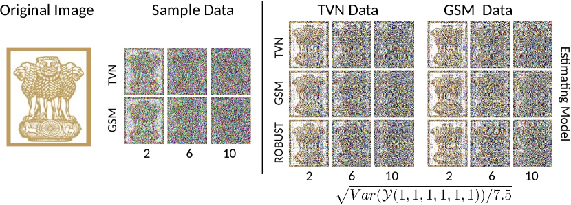
Figure 1: Left block: The Lion capital of Ashoka that is the ground truth of the rearranged mean tensor $\mathcal{M}$ of size $7\times 9\times 3\times 23\times 7\times 3$, and sample realization with increasing variance across two EC distributions. Right block: Estimated $\mathcal{M}$ asuming TVN, GSM models and Tyler’s robust estimators, under TVN and GSM-simulated data. The GSM model-assumed and Tyler estimators perform similarly as the TVN model-assumed estimators for TVN-simulated data, but better than the latter for GSM-simulated data.

We simulated $\Sigma_{k}$ (for $k=1,2,\dots,6$) from $\mathcal{W}_{m_{k}}(100m_{k},I_{m_{k}})$ or a Wishart distribution, before constraining its condition numbers to be at most 50 and scaling each entry by its $(1,1)$th element. The tensor-valued $\mathcal{M}$ was chosen such that when rearranged in a 3-way tensor of size $(7\times 9\times 3)\times(23\times 7)\times 3$, it corresponds to the three RGB slices of a $189\times 161$ true color image of the Lion Capital of Ashoka, shown in the leftmost image of Figure 1.

We also simulated data for $\sigma\in\{2,6,10\}$ and for the TVN case that is a special case of (5) when $\operatorname{{\mathbb{P}}\mbox{r}}(Z_{i}=1)=1$ for all $i=1,\dots,n$. Since $\operatorname{{\mathbb{V}}\mbox{ar}}(\operatorname{vec}(\bm{\mathcal{Y}}_{i}))=15\sigma^{2}\Sigma$, we set $\sigma^{2}$ for TVN-simulated data to be 15 times that of the GSM-simulated cases for both sets to have comparable overall variability. Figure 1 (second set of images in the left block) displays simulated realizations at each setting: as expected, increasing $\sigma^{2}$ produces noisier images. Figure 1 (right block) displays TVN-, GSM- and robust-estimated $\mathcal{\widehat{M}}$s. For Tyler’s robust estimator we used the location estimation procedure of Section III-E. For all cases, estimation performance worsens with increasing $\sigma$. For TVN-simulated data, there is little difference in the quality of $\mathcal{\widehat{M}}$ obtained by the three methods. But for heavy-tailed GSM-simulated data, the GSM or robust $\mathcal{\widehat{M}}$s recover $\mathcal{M}$ better than the TVN-estimated $\mathcal{\widehat{M}}$.

Our illustration in Figure 1 was only on one realization for each setting, so we account for simulation variability in a larger study under a similar framework. We generated TVN and GSM data for $\sigma=2,6,10$ and 100 different realizations of $(\Sigma_{1},\Sigma_{2},\dots,\Sigma_{6})$, each drawn as before from a Wishart distribution.

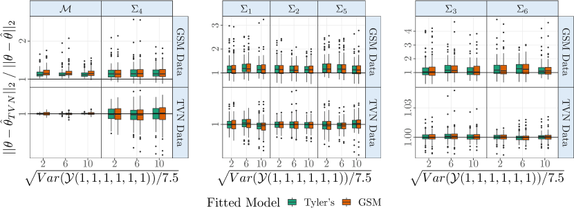
Figure 2: Relative Frobenius norms of differences in parameters (generically denoted by $\theta$) for $\sigma\in\{2,6,10\}$, TVN- and GSM-simulated data, and estimates obtained under Tyler’s robust and GSM model assumptions. Each plot is obtained over 100 realizations from the GSM and TVN models with different values of $\Sigma$s, themselves independent Wishart realizations. All points are concentrated around 1 for TVN-simulated data, indicating that the GSM and Tyler’s estimates perform at least as well as the TVN model when the data is TVN-simulated. For the higher dimensional parameters $\mathcal{M}$ and $\Sigma_{4}\in\mathbb{R}^{23\times 23}$ and for GSM-simulated data, nearly all points are above 1, indicating that the GSM and Tyler’s models outperform the TVN model in this scenario. For medium-sized parameters $\Sigma_{1},\Sigma_{2}\in\mathbb{R}^{7\times 7}$ and $\Sigma_{5}\in\mathbb{R}^{9\times 9}$ and for GSM-simulated data, most points are also larger than 1. However, for the smaller $3\times 3$ matrices $\Sigma_{3}$ and $\Sigma_{6}$ and for GSM-simulated data, the points are more concentrated at around 1. In conclusion, the GSM and Tyler’s models perform at least as well as the TVN model for TVN-simulated data. Morover, the GSM and Tyler’s models outperform the TVN model for GSM-simulated data, and their relative performance increase with larger covariance matrices.

Figure 2 displays the relative Frobenius norms of the difference between the true $(\mathcal{M},\Sigma_{1},\Sigma_{2},\dots,\Sigma_{6})$ and the estimated $(\widehat{\mathcal{M}},\widehat{\Sigma}_{1},\widehat{\Sigma}_{2},\dots,\widehat{\Sigma}_{6})$ parameters, obtained under the GSM, TVN and Tyler models, and for 100 independent samples realized under GSM and TVN assumptions. Specifically, the relative Frobenius normed difference is $R_{d}=||\theta-\widehat{\theta}_{TVN}||_{2}/||\theta-\widehat{\theta}||_{2}$, where $\theta$ generically denotes the parameter being compared, $\widehat{\theta}_{TVN}$ corresponds to the estimated parameter under the TVN model and $\widehat{\theta}$ denotes the estimate of the parameter obtained under the assumed GSM or Tyler’s model. Therefore, values larger than unity indicate better performance of the GSM (or Tyler) estimator over that obtained under TVN assumptions. Conversely, values lower than unity indicate worse performance of GSM (or Tyler) estimates than those obtained under TVN assumptions. Our display in Figure 2 is grouped by parameters of similar dimensionality, with the first plot displaying results for $\mathcal{M}$ and $\Sigma_{4}\in\mathbb{R}^{23\times 23}$, the second one for $\Sigma_{1},\Sigma_{5}\in\mathbb{R}^{7\times 7}$ and $\Sigma_{2}\in\mathbb{R}^{9\times 9}$, and the last one for displaying values of the $3\times 3$ matrices $\Sigma_{3}$ and $\Sigma_{6}$. For TVN-simulated data, there is not much to choose from betwen the TVN-assumed estimates and those obtained using GSM or Tyler estimators. On the other hand, for GSM-simulated data and the higher dimensional parameters $\mathcal{M}$ and $\Sigma_{4}$, the robust GSM and Tyler models outperform the TVN model, since nearly all values exceed unity. The performance of the TVN model is still worse for $\Sigma_{1},\Sigma_{2},\Sigma_{5}$ when compared to the GSM and Tyler models, since $R_{d}$ is then mostly above 1. However, for smaller $3\times 3$ covariance matrices ($\Sigma_{3}$ and $\Sigma_{6}$), the TVN model performs more like the GSM and Tyler models. In conclusion, the GSM and Tyler fits perform similarly to the TVN model for TVN-simulated data. Morover, the GSM and Tyler models outperform the TVN model when the data are GSM-simulated, and their performance relative to the TVN increase with larger covariance matrices. Our simulation experiment shows the importance of considering an EC distribution that is more general than the TVN when the tails of the data are heavier. It also shows the benefit of using Tyler’s robust estimator even when the exact EC distribution is unknown.

V Applications to Image Learning

We apply our EC tensor-variate estimation methodology to two learning applications involving images. The first application is in the context of improved prediction of an image class using tensor-variate discriminant analysis and classification while the second application characterizes the distinctiveness of face images in terms of gender, age and ethnic origin. In each case, the EC distribution with heavier tails (here, the TV-$t$ distribution) is demonstrated to have better results than its TVN counterpart.

V-A Discriminant analysis for image classification

In this section, we provide a general linear (LDA) and quadratic (QDA) framework for the classification of tensor-valued data, in a similar manner as done for vector- [64] and matrix-variate [7] data. We also illustrate how our maximum likelihood estimation methods of Section III are incorporated into the LDA and QDA frameworks, and the benefit of using a more general EC tensor-variate distribution than the TVN in predicting images of dogs or cats in a two-class digital image classification problem. The development of linear and quadratic discriminant analysis is straightforward, so we refer to Section S2-A for details. The methods in Section III are used to estimate the parameters in each class population. Our framework can extend other discriminant analysis methods that considered the normal distribution [65].

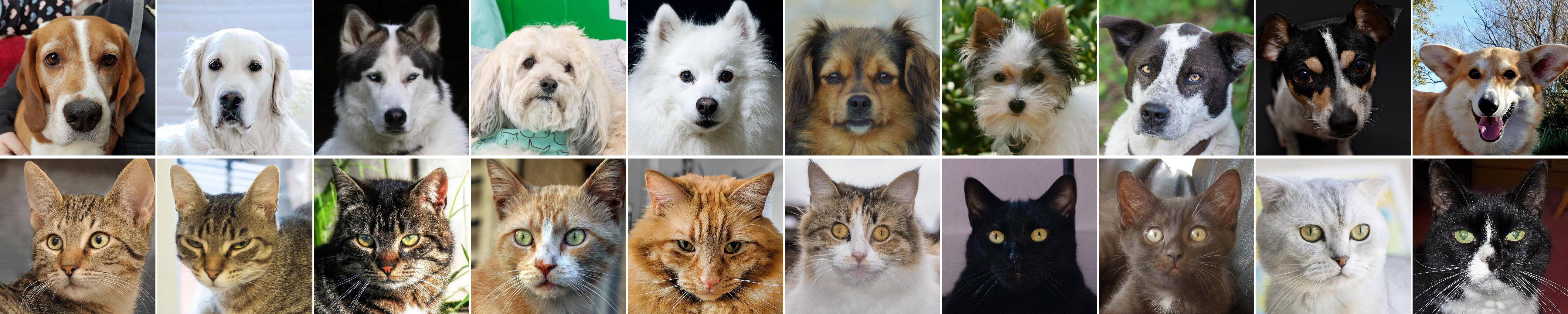
(a)

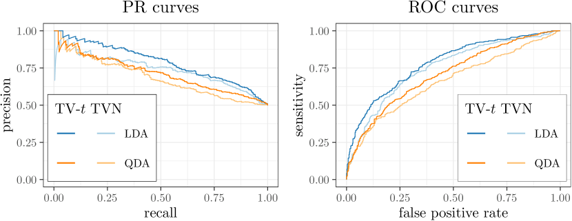
(b)

Figure 3: (a) sample dog and cat images from the AFHQ dataset, (b) precision-recall (PR) and receiver operating characteristic (ROC) curves for the tensor-variate-$t$ (TV-$t$) model and the TVN model, and across both LDA and QDA classification frameworks. The TV-$t$ model outperforms the TVN model in terms of ROC and PR, since the curves corresponding to the TV-$t$ model are higher than those that correspond to the TVN model.

The Animal Faces-HQ (AFHQ) dataset [66] has 15,000 512$\times$512 digital photographs of wild and domestic felines and canines. In this paper, we use our developed methodology to perform classification on the 5,653 cat and 5,239 dog images from the AFHQ dataset, of which 500 images of each animal are test datasets [66]. Figure 3a shows images of ten randomly selected dogs and cats from the database. Despite the attempts at alignment, the images have dissimilar lighting conditions and viewing angles, so we sequentially applied the Radon [67] and 2D discrete wavelet transforms (DWT) [68] to the data in each of the RGB channels and extracted the low-frequency (LL) components [69, 70], yielding a $22\times 22\times 3$ array of features for each training and test image. Figure S2 displays the sequentially applied Radon and DWT transforms that correspond to the cat and dog images of Figure 3a. The processing extracts the local and directional features in the images, with the Radon transform improving the low-frequency components [70] that are then extracted by the wavelet transform [69]. We use QDA and LDA to build discriminant rules from these transformed array data, by modeling each population of transformed images via the TV-$t$ distribution with unknown DF, and for comparison, also the TVN distribution. In particular, we fit

$$\mathcal{Y}_{i}=\langle\bm{x}_{i}|\mathcal{B}\rangle+\mathcal{E}_{i},\quad\mathcal{E}_{i}\sim t_{22,22,3}(\nu;0,\sigma^{2}\Sigma_{1},\Sigma_{2},\Sigma_{3}),$$ (21)

where $\mathcal{Y}_{i}\in\mathbb{R}^{22\times 22\times 3}$ is the $i$th transformed image and $\bm{x}_{i}$ is $[1,0]^{\prime}$ or $[0,1]^{\prime}$ depending on whether $\mathcal{Y}_{i}$ is a transformed image of a cat or a dog. The tensor-variate errors $\mathcal{E}_{i}$ are set to follow a TV-$t$ distribution with unknown $\nu$ DF, which corresponds to the GSM distribution of (6) for $a=b=\nu$. Based on our model (21), the densities $f_{cat}$ and $f_{dog}$ involved in the classification rule of (S7) correspond to the EC distributions $t_{22,22,3}(\nu_{cat};\mathcal{B}_{cat},\sigma^{2}\Sigma_{1},\Sigma_{2},\Sigma_{3})$ and $t_{22,22,3}(\nu_{dog};\mathcal{B}_{dog},\sigma^{2}\Sigma_{1},\Sigma_{2},\Sigma_{3})$, where $\mathcal{B}_{cat}=\mathcal{B}\times_{1}[1,0]$ and $\mathcal{B}_{dog}=\mathcal{B}\times_{1}[0,1]$ are the mean parameters of the transformed cat and dog image populations. Similarly for QDA, we estimate $f_{cat}$ and $f_{dog}$ by fitting $t_{22,22,3}(\nu_{cat};\mathcal{B}_{cat},\sigma^{2}\Sigma_{1},\newline \Sigma_{2},\Sigma_{3})$ and $t_{22,22,3}(\nu_{dog};\mathcal{B}_{dog},\sigma^{2}\Sigma_{1},\Sigma_{2},\Sigma_{3})$ models using the ToTR methodology of (21) with $\bm{x}_{i}\equiv 1$ always.

These models (one for LDA and two for QDA) were fit to the training set images of $5153$ cats and $4739$ dog images using the ECME algorithm of Section III-D. The DFs $\nu$ were estimated using the either step of (16) to be $\nu=3.33$ for the LDA case, and $\nu_{cat}=3.05$ and $\nu_{dog}=3.51.$ We specified $\Sigma_{1}$ and $\Sigma_{2}$ to be AR(1) correlation matrices to capture spatial context in the transformed images, and $\Sigma_{3}$ to have an equicorrelation structure to denote correlation between the three RGB channels. This autocorrelation was estimated to be 0.94 for the LDA case and the same for the cat transformed images but marginally lower (0.93) for the dogs in the QDA fits. We also imposed low-rank CP formats on $\mathcal{B}$, with ranks chosen from among five candidates using cross validation (CV) on the training data, and both missclassification rate and area under the curves (AUC) as our CV decision criteria. For comparison, we also performed QDA and LDA under the TVN model.

The classification rule of (S7) for a transformed image $\mathcal{Y}$ is specified in terms of the loglikelihood ratio (LLR) $=\log(f_{cat}(\mathcal{Y}))-\log(f_{dog}(\mathcal{Y}))+log(\eta_{1}/\eta_{2})$. A large LLR value indicates high posterior probability that $\mathcal{Y}$ is a cat image, with small LLR values conversely indicating high posterior probability that $\mathcal{Y}$ is the image of a dog. A zero value indicates complete uncertainty in the classification. In our application, we set $\eta_{1}=\eta_{2}=0.5$. We obtained posterior logit-probabilities for the $500$ cat and $500$ dog images in the test set, and used them to calculate the precision-recall (PR) curves [71] and the receiver operating characteristic (ROC) curves [72, 73] of Figure 3b. We observe that for both LDA and QDA, PR curves are higher with the TV-$t$ than with the TVN models. This means that there is higher precision at all possible recall values using the TV-$t$ model than the TVN model. In the QDA PR curves, the TVN model sometimes has higher precision than the TV-$t$ model (for recall values of less than 0.2). However, thresholds with recall values of less than 0.2 are not practical, since they lead false negatives (that is, cat images being classified as dog images) to be four times more numerous than true positives (correctly classified cat images). Similarly, in all cases the ROC curve is higher for the TV-$t$ model than for the TVN model. Higher ROC curves mean that all possible false positive rates have higher sensitivity (true positive rate) for the TV-$t$ than for the TVN case. We finish this section noting that $\nu$ was estimated to be less than 3.6 in all cases, meaning that our tensor-variate data are quite heavy-tailed. This explains why the TV-$t$ outperforms the TVN distribution in terms of classification for this real-data example, since it is able to accommodate the heavier tails of the transformed image data.

V-B Distinguishing facial characteristics

The LFW database is commonly used in the development and testing of facial recognition methods [74], and consists of over 13,000 $250\times 250$ color images. Each image has the labeled attributes of ethnic origin, age group and gender [75, 76]. We use our ToTR methodology of Section III-D to distinguish the visual characteristics of different attributes. Specifically, we perform a 3-way tensor-variate analysis of variance (TANOVA) model to distinguish faces across the three factors of gender (male or female), continent of ethnic origin (African, European or Asian, as specified in the database), and cohort (child, youth, middle-aged or senior). Of the more than 13,000 images in the LFW database, we use the 605 images with unambiguous genders, age group and ethnic origin, and with at most 33 images for each factor combination that were selected and made available by [18]. The authors also cropped the images to a central region of size $151\times 111$ each, and logit-transformed them to match the statespace of the normal distribution. In this application, we evaluate whether the use of a model with TV-$t$ errors can provide a more improved fit of the model.

We fit the 3-way TANOVA model with TV-$t$ errors:

$$\mathcal{Y}_{ijkl}=\langle\mathcal{X}_{ijk}|\mathcal{B}\rangle+\mathcal{E}_{ijkl},\quad\mathcal{E}_{ijkl}\sim t_{\bm{m}_{3}}(\nu;0,\sigma^{2}\Sigma_{1},\Sigma_{2},\Sigma_{3}),$$ (22)

where $\bm{m}_{3}=[151,111,3]^{\prime}$ and $\mathcal{Y}_{ijkl}\in\mathbb{R}^{151\times 111\times 3}$ is the 151$\times$111 RGB color image that corresponds to the $l$th person of the $i$th gender, $j$th ethnic origin and $k$th age group $(i=1,2;j=1,2,3;k=1,2,3,4;l=1,\!\hbox to10.00002pt{.\hss.\hss.},n_{ijk})$. Here $\mathcal{X}_{ijk}\in\mathbb{R}^{2\times 3\times 4}$ is the tensor-valued covariate with 1 at position $(i,j,k)$ and zero elsewhere, and indicates the factor combination of $\mathcal{Y}_{ijk}$. The regression coefficient $\mathcal{B}\in\mathbb{R}^{2\times 3\times 4\times 151\times 111\times 3}$ contains the group means across all factor combinations. As in Section V-A, we constrain $\Sigma_{1}$ and $\Sigma_{2}$ to be AR(1) correlation matrices and $\Sigma_{3}$ to be an equicorrelation matrix. We fit our model (22) assuming TV-$t$ errors with unknown DF parameter $\nu$ and TVN errors. The DF $\nu$ was estimated in all cases, and for ultra heavy-tailed data $\nu$ was constrained to never be lower than 2.01, so that that the first two population moments exist. Such is the case for this LFW dataset, which selected $\widehat{\nu}=2.01$ as the DF in all cases. We also fit the model assuming two different assumptions on the $\mathcal{B}$: the CP format, the TT format [58] that is the tensor-ring (TR) format [59] when one of the TR ranks is set to 1. We also assumed an unconstrained $\mathcal{B}$ (with no reduction in the number of parameters). We chose the CP and TT ranks using the Bayesian Information Criterion (BIC) [77, 78] out of a total of 26 candidate ranks (for CP), and from nine ranks for the TT format. The chosen CP rank was $R=70$, with 19,175 unconstrained parameters in $\mathcal{B}$, or a 98.4% dimension reduction relative to the unconstrained $\mathcal{B}$ that contains more than 1.2 million parameters. The TT rank was chosen to be $g=(1,2,4,8,4,2)$, which resulted in a total of 8,450 unconstrained parameters in $\mathcal{B}$, or a 99% dimension reduction relative to the unconstrained $\mathcal{B}$. Table II displays the BICs across the six (two error distributions across three $\mathcal{B}$ formats) assumptions.

TABLE II: BICs for different fits, with smaller values indicating better model fit. The TV-$t$ fits in this table and this paper have a selected DF parameter $\nu$ of 2.01, which in all cases outperformed their TVN counterparts.

		Format of $\mathcal{B}$
		TT	CP	none
Error Model	TVN	-11,190,861	-11,223,595	-4,745,807
	TV-$t$	-23,992,185	-24,064,833	-20,043,342

From Table II, we observe that the TV-$t$ distribution always outperforms its TVN counterpart, which indicates the benefit of considering a model for the heavy tails. Moreover, within the TVN or TV-$t$ models, the CP and TT formats always outperform the model with unconstrained $\mathcal{B}$, with the CP always performing better than the TT. This shows the benefit of using a low-rank format that allows massive parameter reductions while also preserving model accuracy. Importantly in the context of this paper, we find that the TV-$t$ distributions with constrained or unconstrained $\mathcal{B}$ outperform all the TVN models, including the TT and CP formats. Our findings show that performing parameter reduction through the CP or TT low-rank formats should be accompanied with the more appropriate model for the tail weights. Indeed, the best performance is achieved when the low-rank format is used in combination with the heavy-tailed TV-$t$ distribution.

(a) TV-$t$

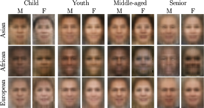
(b) TVN

Figure 4: Different slices of the resulting factorized tensor $\mathcal{B}$ that results from fitting the ToTR model on a 3-way factor ANOVA of the LFW dataset using the CP format and the (a) TV-$t$ distribution and (b) TVN distribution. The results are CP-format compressed mean images across age groups (child, youth, middle aged and senior), ethnic origin (Asian, African, European) and genders (male, female) from the 605 LFW images used in [18]. The imposed CP format preserved vital information regarding the factor-combination of age group, gender and ethnic-origin while providing substantial (more than $98\%$) parameter reduction.

Figures 4a and 4b display the estimated $\mathcal{\widehat{B}}$ for the TV-$t$ ($\nu=2.01$) and TVN models. In both cases, the CP format preserves vital visual characteristics regarding ethnic origin, gender, and age-group. However, the TVN formatted $\mathcal{B}$ results in more exaggerated facial expressions, while the fits under the TV-$t$ model are sometimes noisier, but more accurately reflect the diversity of facial characteristics in each sub-group. Therefore, we contend that the TV-$t$ model not only provides a quantitatively better fit to the TANOVA model, but also more accurately displays the heterogeneity in the dataset.

VI Discussion

In this article, we introduced, defined, characterized and studied in detail the family of spherically and EC tensor-variate distributions that generalize the well-studied TVN distributions. We derived CFs, PDFs, exact distributions of linear reshapings, linear transformations, derived the moments of different orders as well as of special forms, and introduced the EC tensor-variate Wishart distribution. These properties arise not only from the vectorized elliptical form of the random tensor, but also from its intrinsic tensor-variate structure, which in many cases makes estimation and inference possible. We provided algorithms for maximum likelihood estimation under different assumptions on the observed EC data. First, we suggested a modification to the maximum likelihood estimation algorithm for TVN data that makes its parameter estimates identifiable. We then use this algorithm to propose a maximum likelihood estimation algorithm for uncorrelated EC tensor-valued observations. We also derive EM algorithm variants for maximum likelihood estimation under IID draws from a scale mixture of TVN distribution, and a novel, robust and constrained Tyler-type algorithm for maximum likelihood estimation when the underlying EC tensor-variate distribution is unknown. We further proposed a ToTR framework with EC errors that extends the work of [18] to the case where the tensor-response regression has EC tensor-variate distributed errors under various low-rank format assumptions on the regression coefficient. We studied the performance of our estimation algorithms through a simulation experiment on 6-way tensor-valued data that showed the limitations of the TVN distribution when the data have heavier tails than can be modeled by the TVN. Indeed, we demonstrated that fitting a GSM or Tyler robust estimating model to such data results in improved performance when the data is not Gaussian. Further, we provided methodology that allows us to use our maximum likelihood methodology to perform LDA and QDA on tensor-data classification and discrimination, and applied it to predict images of cats or dogs in the AFHQ dataset. We demonstrate that the AFHQ data is quite heavy-tailed, resulting in better performance for the TV-$t$ model relative to the TVN model in terms of ROC and PR curves. Finally, we used our ToTR methodology to perform a 3-way TANOVA of facial images from the LFW database. We demonstrate that the database is exceptionally heavy-tailed (with a selected DF of 2.01), since the TV-$t$ models outperfom their TVN counterparts in all scenarios.

There are several possible extensions and generalizations of our work. First, we can define spherical distributions in multiple ways. The class of distributions $\mathscr{F}_{k}=\{\bm{\mathcal{X}}\!:\!\bm{\mathcal{X}}\overset{d}{=}[\![\bm{\mathcal{X}};\Gamma_{1},\!\hbox to10.00002pt{.\hss.\hss.}\Gamma_{k},I_{m_{k+1}},\newline \!\hbox to10.00002pt{.\hss.\hss.},I_{m_{p}}]\!]$, $\Gamma_{j}\in O(m_{j})\forall j\in\{1,\!\hbox to10.00002pt{.\hss.\hss.},k\}\}$ is such that $\mathscr{F}_{A}\subseteq\mathscr{F}_{p}\subseteq\mathscr{F}_{p-1}\subseteq\!\hbox to10.00002pt{.\hss.\hss.}\subseteq\mathscr{F}_{1},$ where $\mathscr{F}_{A}$ is the family we defined in this article. All these families have Kronecker-separable covariance structures if the family of EC random tensors is defined using the Tucker product, as in (4). The Kronecker-separable structure makes it practical for us to explore the parameter space of the ultra-high dimensional covariance matrix. However, other types of variance structures can also be considered. Finally, the sampling distributions of $\mathcal{B}$ in our ToTR with EC errors are unknown, and may be of interest in applications where significance testing is important. Thus, we see that though we have developed theory and estimation methodology for EC tensor-variate distributions, there remain a number of extensions and generalizations that are worthy of investigation.

Supplementary Appendix

S1 Supplement to Section 2

S1-A Tensor algebra notation involved in Section II-A

As in Section II-A, we assume $\mathcal{X}$ is a $p-$way tensor of size $m_{1}\times m_{2}\times\ldots\times m_{p}$ and $\bm{e}_{i}^{m}\in\mathbb{R}^{m}$ is a unit-basis vector with 1 as the $i$th element and 0 elsewhere. The vector outer product of a set of vectors $(\bm{z}_{1},\bm{z}_{2},\ldots,\bm{z}_{p})$, where $\bm{z}_{j}\in\mathbb{R}^{n_{j}}$ for all $j=1,2,\ldots,p$, is written as $\operatorname*{\circ}_{j=1}^{p}\bm{z}_{j}$ and results in a $p-$way tensor of size $n_{1}\times n_{2}\times\ldots\times n_{p}$ such that $(\operatorname*{\circ}_{j=1}^{p}\bm{z}_{j})(i_{1},i_{2},\ldots,i_{p})=\prod_{j=1}^{p}\bm{z}_{j}(i_{j}).$ This product is useful for expressing $\mathcal{X}$ as

$$\sum_{i_{1}=1}^{m_{1}}\ldots\sum_{i_{p}=1}^{m_{p}}\mathcal{X}(i_{1},i_{2},\ldots,i_{p})\big{(}\operatorname*{\circ}_{q=1}^{p}\bm{e}_{i_{q}}^{m_{q}}\big{)},$$ (S1)

and the Tucker product between $\mathcal{X}$ and ${\sf A}_{1},{\sf A}_{2},$ $\ldots,{\sf A}_{p}$ as

$$[\![\mathcal{X};{\sf A}_{1},{\sf A}_{2},\ldots,{\sf A}_{p}]\!]=\sum_{i_{1}\dots i_{p}}\mathcal{X}(i_{1},i_{2},\ldots,i_{p})\big{(}\operatorname*{\circ}\limits_{q=1}^{p}{\sf A}_{q}(:,i_{q})\big{)},$$

where ${\sf A}_{q}(:,i_{q})$ is the $i_{q}$th column of ${\sf A}_{q}$. Tensor reshapings are obtained by manipulating the vector outer product. We define the vectorization, $k$th mode matricization and $k$th canonical matricization of $\mathcal{X}$ as

$$\operatorname{vec}(\mathbf{\mathcal{X}})=\sum\limits_{i_{1}=1}^{m_{1}}\ldots\sum\limits_{i_{p}=1}^{m_{p}}\mathcal{X}(i_{1},i_{2},\ldots,i_{p})\big{(}\bigotimes\limits_{q=p}^{1}\bm{e}_{i_{q}}^{m_{q}}\big{)},$$ (S2)

$$\mathcal{X}_{(k)}=\sum\limits_{i_{1}=1}^{m_{1}}\ldots\sum\limits_{i_{p}=1}^{m_{p}}\mathcal{X}(i_{1},i_{2},\ldots,i_{p})\bm{e}_{i_{k}}^{m_{k}}\big{(}\bigotimes\limits_{q=p,q\neq k}^{1}\bm{e}_{i_{q}}^{m_{q}}\big{)}^{\prime},$$ (S3)

$$\mathcal{X}_{<k>}=\sum\limits_{i_{1}=1}^{m_{1}}\ldots\sum\limits_{i_{p}=1}^{m_{p}}\mathcal{X}(i_{1},i_{2},\ldots,i_{p})\big{(}\bigotimes\limits_{q=k}^{1}\bm{e}_{i_{q}}^{m_{q}}\big{)}\big{(}\bigotimes\limits_{q=p}^{k+1}\bm{e}_{i_{q}}^{m_{q}}\big{)}^{\prime},$$ (S4)

respectively for any $k=1,2,\ldots,p$. The tensor outer product ($\circ$) between $\mathcal{X}$ and $\mathcal{Y}\in\mathbb{R}^{n_{1}\times n_{2}\times\ldots\times n_{q}}$ results in a tensor $\mathcal{X}\circ\mathcal{Y}$ of size $(m_{1}\times m_{2}\times\ldots\times m_{p}\times n_{1}\times n_{2}\times\ldots\times n_{q})$ such that $(\mathcal{X}\circ\mathcal{Y})(i_{1},i_{2},\ldots,i_{p},j_{1},j_{2},\ldots,j_{q})=\mathcal{X}(i_{1},i_{2},\ldots,i_{p})\mathcal{Y}(j_{1},j_{2},\ldots,j_{q}).$ With the tensor outer product defined, we now state and prove

Lemma 12.

Let $\bm{\mathcal{Y}}\in\mathbb{R}^{n_{1}\times n_{2}\times\dots\times n_{q}}$. Then $(\bm{\mathcal{X}}\circ\bm{\mathcal{Y}})_{<p>}=(\operatorname{vec}\bm{\mathcal{X}})(\operatorname{vec}\bm{\mathcal{Y}})^{\prime}.$

Proof.

See Section S3-I. ∎

S1-B Marginal distributions

The marginal distributions follow from Theorem 3. by choosing ${\sf A}_{1},{\sf A}_{2},\ldots,{\sf A}_{p}$ appropriately. As an example, consider the 3-way random tensor $\bm{\mathcal{Y}}\sim\operatorname{\mathcal{E}\mathcal{C}}_{m_{1},m_{2},m_{3}}\big{(}\mathcal{M},\Sigma_{1},\Sigma_{2},\Sigma_{3},\varphi\big{)}$, which will be split into eight sub-tensors as

$$\bm{\mathcal{Y}}_{ijk}=[\![\bm{\mathcal{Y}};{\sf A}_{i1},{\sf A}_{j2},{\sf A}_{k3}]\!],\quad\mathcal{M}_{ijk}=[\![\mathcal{M};{\sf A}_{i1},{\sf A}_{j2},{\sf A}_{k3}]\!],$$ (S5)

where ${\sf A}_{1l}=[{\sf I}_{n_{l}}\vdots\bm{0}]$ and ${\sf A}_{2l}=[\bm{0}\vdots{\sf I}_{m_{l}-n_{l}}]$ are block matrices of size $n_{l}\times m_{l}$ and $(m_{l}-n_{l})\times m_{l}$ respectively, and $n_{l}<m_{l}$ for all $l=1,2,3$ and $i,j,k=1,2$ (here ${\sf I}_{h}$ denotes an $h\times h$ identity matrix and $\bm{0}$ is a matrix of zeroes). Figure S1

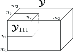
Figure S1: A random third order tensor $\bm{\mathcal{Y}}$ along with one of its subtensors $\bm{\mathcal{Y}}_{111}$.

displays $\bm{\mathcal{Y}}$ along one of its eight sub-tensors $\bm{\mathcal{Y}}_{111}$. Using Theorem 3 and (S5), we obtain its marginal distribution as

$$\bm{\mathcal{Y}}_{111}\sim\operatorname{\mathcal{E}\mathcal{C}}_{n_{1},n_{2},n_{3}}\big{(}\mathcal{M}_{111},{\sf A}_{11}\Sigma_{1}{\sf A}_{11}^{\top},{\sf A}_{12}\Sigma_{2}{\sf A}_{12}^{\top},{\sf A}_{13}\Sigma_{3}{\sf A}_{13}^{\top},\varphi\big{)},$$

where ${\sf A}_{1k}\Sigma_{k}{\sf A}_{1k}^{\top}$ is a sub-matrix corresponding to the first $n_{k}$ columns and rows of $\Sigma_{k}$.

S1-C Conditional distributions along multiple modes

Here we demonstrate how to find conditional distribution along multiple modes. As an example, consider the subtensor $\bm{\mathcal{Y}}_{111}$ of $\bm{\mathcal{Y}}\sim\operatorname{\mathcal{E}\mathcal{C}}_{m_{1},m_{2},m_{3}}\big{(}\mathcal{M},\Sigma_{1},\Sigma_{2},\Sigma_{3},\varphi\big{)}$, both shown in Figure S1 and let

$$\Sigma_{i}=\begin{bmatrix}\Sigma_{i,11}&\Sigma_{i,12}\\ \Sigma_{i,21}&\Sigma_{i,22}\end{bmatrix},\quad\Sigma_{i,11}\in\mathbb{R}^{n_{i}\times n_{i}},$$

and $\Sigma_{i,\{11\}|\bullet}=\Sigma_{i,11}-\Sigma_{i,12}\Sigma_{i,22}^{-1}\Sigma_{i,21}$ for $i=1,2,3$. Then

$$\mathcal{L}(\bm{\mathcal{Y}}_{111}\big{|}\bm{\mathcal{Y}}_{\backslash\{111\}}=\mathcal{Y}_{\backslash\{111\}})=\operatorname{\mathcal{E}\mathcal{C}}_{n_{1},n_{2},n_{3}}\big{(}\mathcal{M}_{\{111\}|\textbackslash\{111\}},\Sigma_{1,\{11\}|\bullet},\Sigma_{2,\{11\}|\bullet},\Sigma_{3,\{11\}|\bullet},\varphi_{q}\big{)},$$

where the event $\bm{\mathcal{Y}}_{\backslash\{111\}}=\mathcal{Y}_{\backslash\{111\}}$ means that $\bm{\mathcal{Y}}_{112}=\mathcal{Y}_{112},\bm{\mathcal{Y}}_{121}=\mathcal{Y}_{121},\bm{\mathcal{Y}}_{122}=\mathcal{Y}_{122},\bm{\mathcal{Y}}_{211}=\mathcal{Y}_{211},\bm{\mathcal{Y}}_{212}=\mathcal{Y}_{212},\bm{\mathcal{Y}}_{221}=\mathcal{Y}_{221},\mbox{ and }\bm{\mathcal{Y}}_{222}=\mathcal{Y}_{222}$,

$$\begin{split}\mathcal{M}_{\{111\}|\textbackslash\{111\}}&=[\![(\mathcal{Y}_{222}-\mathcal{M}_{222});\Sigma_{1,12}\Sigma_{1,22}^{-1},\Sigma_{2,12}\Sigma_{2,22}^{-1},\Sigma_{3,12}\Sigma_{3,22}^{-1}]\!]\\ +&(\mathcal{Y}_{211}-\mathcal{M}_{211})\times_{1}(\Sigma_{1,12}\Sigma_{1,22}^{-1})-[\![(\mathcal{Y}_{122}\!-\!\mathcal{M}_{122});I_{n_{1}},\Sigma_{2,12}\Sigma_{2,22}^{-1},\Sigma_{3,12}\Sigma_{3,22}^{-1}]\!]\\ +&(\mathcal{Y}_{121}-\mathcal{M}_{121})\times_{2}(\Sigma_{2,12}\Sigma_{2,22}^{-1})-[\![(\mathcal{Y}_{212}-\mathcal{M}_{212});\Sigma_{1,12}\Sigma_{1,22}^{-1},I_{n_{2}},\Sigma_{3,12}\Sigma_{3,22}^{-1}]\!]\\ +&(\mathcal{Y}_{112}-\mathcal{M}_{112})\times_{3}(\Sigma_{3,12}\Sigma_{3,22}^{-1})-[\![(\mathcal{Y}_{221}-\mathcal{M}_{221});\Sigma_{1,12}\Sigma_{1,22}^{-1},\Sigma_{2,12}\Sigma_{2,22}^{-1},I_{n_{3}}]\!],\end{split}$$

and $\varphi_{q}(u)=\mathbb{E}\left(R^{2}_{q}\varphi_{\bm{\mathcal{U}}}(u)\mid\bm{\mathcal{Y}}_{\backslash\{111\}}=\mathcal{Y}_{\backslash\{111\}}\right),$ with $R^{2}_{q}=D^{2}_{\Sigma_{3,\{11\}|\bullet}\otimes\Sigma_{2,\{11\}|\bullet}\otimes\Sigma_{1,\{11\}|\bullet}}(\bm{\mathcal{Y}}_{111},\allowbreak\mathcal{M}_{111}),$. If $\varphi(u)=\exp(-u/2)$, then the conditional distribution of $R^{2}_{q}$ given $\bm{\mathcal{Y}}_{\backslash\{111\}}=\mathcal{Y}_{\backslash\{111\}}$ is $\chi^{2}_{n_{1}n_{2}n_{3}}$, and $\varphi_{q}(u)=\exp(-u/2)$.

S1-D The Singular EC Wishart distribution

Suppose $\bm{{\sf X}}\sim\operatorname{\mathcal{E}\mathcal{C}}_{m,n}(0,\Sigma,I_{n},\varphi)$ for $n<m$. Then $\bm{{\sf S}}=\bm{{\sf X}}\bm{{\sf X}}^{\top}\sim\operatorname{\mathcal{E}\mathcal{C}\mathcal{W}}_{m}(n,\Sigma,\varphi)$ but $\bm{{\sf S}}$ is singular. In the following we extend the results of [79, 80] to obtain the joint PDF of the functionally independent elements of $\bm{{\sf S}}$.

Theorem 13.

Suppose $\bm{{\sf S}}\sim\operatorname{\mathcal{E}\mathcal{C}\mathcal{W}}_{m}(n,\Sigma,\varphi),$ with $n<m$, and for the $n\!\times\!n$ matrix $\bm{{\sf S}}_{11}$,

$$\bm{{\sf S}}=\begin{bmatrix}\bm{{\sf S}}_{11}&\bm{{\sf S}}_{12}\\ \bm{{\sf S}}_{12}^{\top}&\bm{{\sf S}}_{22}\end{bmatrix}.$$

Then the joint PDF of the functionally independent elements of $\bm{{\sf S}}$ is

$$f_{[\bm{{\sf S}}_{11}\bm{{\sf S}}_{12}]}({\sf S})=\dfrac{\pi^{n^{2}/2}}{\Gamma_{n}(n/2)|\Sigma|^{n/2}}|{\sf S}_{11}|^{(n-m-1)/2}g(\operatorname{tr}(\Sigma^{-1}{\sf S})).$$ (S6)

Proof.

See Section S3-J. ∎

S2 Supplement to Section 4

S2-A Linear and quadratic tensor-variate classification

Consider $G$ tensor-valued populations $\pi_{1},\pi_{2},\dots,\pi_{G}$. A Bayes-optimal rule that minimizes the total probability of missclassification assigns an observed tensor $\mathcal{X}$ to group $\pi_{i^{*}}$ if $i^{*}=\operatorname*{arg\,max}_{i=1,\dots,G}\eta_{i}f_{i}(\mathcal{X})$, where $f_{i}(\mathcal{X})$ is the PDF of $\pi_{i}$ evaluated at $\mathcal{X}$, and $\eta_{i}$ is the prior probability that a member of $\pi_{i}$ gets correctly classified [64, 7].

We first briefly visit the two-class problem. Here, we consider two tensor-valued populations $\pi_{1}$ and $\pi_{2}$. For $i,j=1,2$ let $\eta_{i}$ be the prior probability that a member of $\pi_{i}$ gets correctly classified to $\pi_{i}$, and also let $\mathbb{P}(i|j)$ be the probability that a member of $\pi_{j}$ gets misclassified to $\pi_{i}$ $(i\neq j)$. The total probability of misclassification (TPM) in this case is $\mathbb{P}(2|1)\eta_{1}+\mathbb{P}(1|2)\eta_{2}$. Now, suppose we are interested in classifying one tensor-valued observation $\mathcal{X}$ to $\pi_{1}$ or $\pi_{2}$. In this case, a Bayes-optimal rule that minimizes the TPM assigns $\mathcal{X}$ to $\pi_{1}$ if $\eta_{1}f_{1}(\mathcal{X})\geq\eta_{2}f_{2}(\mathcal{X})$, where $f_{i}(\mathcal{X})$ is the PDF of group $\pi_{i}$ evaluated at $\mathcal{X}$ [64, 7].

The extension of this rule to the case where there are $G$ groups $\pi_{1},\pi_{2},\dots,\pi_{G}$ assigns $\mathcal{X}$ to $\pi_{i^{*}}$ if $i^{*}=\operatorname*{arg\,max}_{i=1,2,\dots,G}\eta_{i}f_{i}(\mathcal{X})$, where $f_{i}$ and $\eta_{i}$ correspond to the PDF and prior probability that a member of $\pi_{i}$ gets correctly classified, respectively.

Suppose that $\pi_{i}$ has the $\operatorname{\mathcal{E}\mathcal{C}}_{\bm{m}}(\mathcal{M}_{i},\Sigma_{i,1},\!\hbox to10.00002pt{.\hss.\hss.},\Sigma_{i,3},\varphi)$ distribution with PDF (8). Then an observation $\mathcal{Y}$ is assigned to $\pi_{1}$ over $\pi_{2}$ if

$$\eta_{1}|\Sigma_{1}|^{-1/2}g(D^{2}_{\Sigma_{1}}(\mathcal{Y},\mathcal{M}_{1}))\geq\eta_{2}|\Sigma_{2}|^{-1/2}g(D^{2}_{\Sigma_{2}}(\mathcal{Y},\mathcal{M}_{2})),$$ (S7)

where $\Sigma_{i}=\otimes_{k=p}^{1}\Sigma_{i,k}$. This rule is greatly simplified for the TVN case where $g(u)=\pi^{-m/2}\exp(-u/2)$ as

$$\log\left(\dfrac{\eta_{1}^{2}}{\eta_{2}^{2}}\right)\!-\!\log\left(\dfrac{|\Sigma_{1}|}{|\Sigma_{2}|}\right)\!-\!\left(D^{2}_{\Sigma_{1}}(\mathcal{Y},\mathcal{M}_{1})-D^{2}_{\Sigma_{2}}(\mathcal{Y},\mathcal{M}_{2})\right)\!>\!0.$$ (S8)

(S8) is a quadratic discrimination analysis (QDA) classification rule, with the usual reduction to linear discriminant analysis (LDA) for homogeneous covariance structures in the case of GSM distributions with PDF as in (6).

The parameters involved in (S7) can be estimated from a training dataset using the methodology of Section III. Moreover, our ToTR methodology of Section III-D allows us to estimate the mean parameters $\mathcal{M}_{1}$ and $\mathcal{M}_{2}$ under low-rank formats, thereby facilitating substantial parameter reduction in many imaging applications. ML estimates under the homogeneity of variance can be obtained by fitting the TANOVA model

$$\mathcal{Y}_{i}=\langle\bm{x}_{i}|\mathcal{B}\rangle+\mathcal{E}_{i},\quad\mathcal{E}_{i}\sim\operatorname{\mathcal{E}\mathcal{C}}_{\bm{m}}(0,\sigma^{2}\Sigma_{1},\dots,\Sigma_{p},\varphi),$$ (S9)

where $\bm{x}_{i}=[0,1]^{\prime}$ or $\bm{x}_{i}=[1,0]^{\prime}$ accordingly as whether $\mathcal{Y}_{i}\in\pi_{1}$ or $\mathcal{Y}_{i}\in\pi_{2}$. With population-specific covariances, we estimate the parameters in (S7) by fitting separate EC models to the training data from each group using the methods of Section III. For the ToTR under low-rank format case, fitting models to separate groups can be thought as the special case of (S9) when $\bm{x}_{i}$ is the scalar 1. We now illustrate our methodology on images from the AFHQ database.

In section V-A we display the sequentially applied Radon and DWT transforms of the cat and dog images displayed in Figure 3a. These transformed figures are displayed in Figure S2 and are examples of the $\mathcal{Y}$s that are used in the calculation of the decision rule and in the prediction.

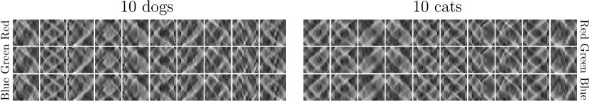
Figure S2: Radon and DWT transforms across the 3 RGB channels for the sample dog and cat images of Figure 3a.

S3 Proofs

S3-A Proof of Theorem 2

Proof.

From the invariance of the Mahalanobis distance under tensor reshapings, $\bm{\mathcal{Y}},\bm{\mathcal{Y}}_{(k)},\bm{\mathcal{Y}}_{<k>}$ and $\operatorname{vec}(\bm{\mathcal{Y}})$ all have the same characteristic function (CF), equivalently written for each case, as

$$\begin{split}\psi_{\bm{\mathcal{Y}}}(\mathcal{Z})\overset{1}{=}&\exp(\imath\langle\mathcal{Z},\mathcal{M}\rangle)\varphi(\langle\mathcal{Z},[\![\mathcal{Z};\Sigma_{1},\Sigma_{2},\ldots,\Sigma_{p}]\!]\rangle)\\ \overset{2}{=}&\exp(\imath\langle\mathcal{Z}_{(k)},\mathcal{M}_{(k)}\rangle)\varphi(\langle\mathcal{Z}_{(k)},[\![\mathcal{Z}_{(k)};\Sigma_{k},\Sigma_{-k}]\!]\rangle)\\ \overset{3}{=}&\exp(\imath\langle\mathcal{Z}_{<k>},\mathcal{M}_{<k>}\rangle)\varphi(\langle\mathcal{Z}_{<k>},[\![\mathcal{Z}_{<k>};\otimes_{q=1}^{k}\Sigma_{q},\otimes_{q=k+1}^{p}\Sigma_{q}]\!]\rangle)\\ \overset{4}{=}&\exp(\imath\langle\operatorname{vec}(\mathcal{Z}),\operatorname{vec}(\mathcal{M})\rangle)\varphi(\langle\operatorname{vec}(\mathcal{Z}),[\![\operatorname{vec}(\mathcal{Z});\Sigma]\!]\rangle).\end{split}$$

∎

S3-B Proof of Theorem 3

Proof.

The CF of $[\![\bm{\mathcal{Y}};{\sf A}_{1},\!\hbox to10.00002pt{.\hss.\hss.},{\sf A}_{p}]\!]$ can be expressed in terms of the CF of $\bm{\mathcal{Y}}$ as $\psi_{\bm{\mathcal{Y}}}([\![\mathcal{Z};{\sf A}_{1}^{\top},\!\hbox to10.00002pt{.\hss.\hss.},{\sf A}_{p}^{\top}]\!])$, and using (7), we have

$$\psi_{\bm{\mathcal{Y}}}([\![\mathcal{Z};{\sf A}_{1}^{\top},\!\hbox to10.00002pt{.\hss.\hss.},{\sf A}_{p}^{\top}]\!])\!=\!\exp(\imath\langle\mathcal{Z},[\![\mathcal{M};{\sf A}_{1},\!\hbox to10.00002pt{.\hss.\hss.},{\sf A}_{p}]\!]\rangle)\varphi(\langle\mathcal{Z},[\![\mathcal{Z};{\sf A}_{1}\Sigma_{1}{\sf A}_{1}^{\top},\!\hbox to10.00002pt{.\hss.\hss.},{\sf A}_{p}\Sigma_{p}{\sf A}_{p}^{\top}]\!]\rangle).$$

The rest of Part 1 of the theorem follows from (7). ∎

S3-C Proof of Theorem 4

Proof.

From Part 4 of Theorem 2, we can write the distribution of $\operatorname{vec}{(\bm{\mathcal{Y}})}$ as

$$\begin{split}\operatorname{vec}{(\bm{\mathcal{Y}})}=\begin{bmatrix}\operatorname{vec}(\bm{\mathcal{Y}}_{1})\\ \operatorname{vec}(\bm{\mathcal{Y}}_{2})\end{bmatrix}\sim\operatorname{\mathcal{E}\mathcal{C}}_{m_{-p}\times(n_{1}+n_{2})}\Big{(}\begin{bmatrix}\operatorname{vec}(\mathcal{M}_{1})\\ \operatorname{vec}(\mathcal{M}_{2})\end{bmatrix},\begin{bmatrix}\Sigma_{11}\otimes\Sigma_{-p}&\Sigma_{12}\otimes\Sigma_{-p}\\ \Sigma_{21}\otimes\Sigma_{-p}&\Sigma_{22}\otimes\Sigma_{-p}\end{bmatrix},\varphi\Big{)}.\end{split}$$

The remainder of the proof follows from Corollary 5 in [27] and Part 1 of Theorem 2, after noticing that $\operatorname{vec}(\mathcal{M}_{\{1\}|\{2\}})=\operatorname{vec}(\mathcal{M}_{1})+(\Sigma_{12}\otimes\Sigma_{-p})(\Sigma_{22}\otimes\Sigma_{-p})^{-1}(\operatorname{vec}(\mathcal{Y}_{2})-\operatorname{vec}(\mathcal{M}_{2}))$ and $\Sigma_{p,\{11\}|\bullet}\otimes\Sigma_{-p}=(\Sigma_{11}\otimes\Sigma_{-p})-(\Sigma_{12}\otimes\Sigma_{-p})(\Sigma_{22}\otimes\Sigma_{-p})^{-1}(\Sigma_{21}\otimes\Sigma_{-p}).$ ∎

S3-D Proof of Theorem 5

The CF of $\bm{\mathcal{Y}}$ in (7) can be written as $\psi_{\bm{\mathcal{Y}}}(\mathcal{Z})=\exp(\imath h(\mathcal{Z}))\varphi(g(\mathcal{Z})),$ where $h(\mathcal{Z})=\langle\mathcal{Z},\mathcal{M}\rangle$ and $g(\mathcal{Z})=\langle\mathcal{Z},[\![\mathcal{Z};\Sigma_{1},\ldots,\Sigma_{p}]\!]\rangle.$ Denote $\mathcal{Z}_{\bm{i}}=\mathcal{Z}(i_{1},\ldots,i_{p})$, the first derivative of $h(\cdot)$ as $\partial h(\mathcal{Z})/\partial\mathcal{Z}_{\bm{i}}=m_{\bm{i}}$, the first derivative of $g(\cdot)$ as $g_{\bm{i}}\overset{.}{=}(\partial h(\mathcal{Z}))/(\partial\mathcal{Z}_{\bm{i}})$, and the second derivative of $g(\cdot)$ as $g_{\bm{i}\bm{j}}\overset{.}{=}\partial^{2}h(\mathcal{Z})/\partial\mathcal{Z}_{\bm{i}}\partial\mathcal{Z}_{\bm{j}}=2\sigma_{\bm{i}\bm{j}}.$ All higher order derivatives are zero. Then

1. The first moment is obtained from $\mathbb{E}(Y_{\bm{i}})=\imath^{-1}\dfrac{\partial\psi_{\bm{\mathcal{Y}}}}{\partial\mathcal{Z}_{\bm{i}}}(0)$, where

   $$\dfrac{\partial\psi_{\bm{\mathcal{Y}}}(\mathcal{Z})}{\partial\mathcal{Z}_{\bm{i}}}=\exp(\imath h(\mathcal{Z}))\big{[}g_{\bm{i}}\varphi^{\prime}(g(\mathcal{Z}))+\imath m_{\bm{i}}\varphi(g(\mathcal{Z}))\big{]}.$$

2. The second moment uses $\mathbb{E}(Y_{\bm{i}}Y_{\bm{j}})=\imath^{-2}\frac{\partial^{2}\psi_{\bm{\mathcal{Y}}}}{\partial\mathcal{Z}_{\bm{i}}\partial\mathcal{Z}_{\bm{j}}}(0)$, where $\frac{\partial^{2}\psi_{\bm{\mathcal{Y}}}}{\partial\mathcal{Z}_{\bm{i}}\partial\mathcal{Z}_{\bm{j}}}(\mathcal{Z})$ is

   $\exp(\imath h(\mathcal{Z}))\times\Bigg{[}\varphi^{\prime\prime}(g(\mathcal{Z}))\big{(}g_{\bm{i}}g_{\bm{j}}\big{)}+\varphi^{\prime}(g(\mathcal{Z}))\big{(}g_{\bm{i}\bm{j}}+\imath g_{\bm{i}}m_{\bm{j}}+\imath g_{\bm{j}}m_{\bm{i}}\big{)}+\varphi(g(\mathcal{Z}))\big{(}\imath^{2}m_{\bm{i}}m_{\bm{j}}\big{)}\Bigg{]}.$

3. The third moment is obtained using $\mathbb{E}(Y_{\bm{i}}Y_{\bm{j}}Y_{\bm{k}})=\imath^{-3}\frac{\partial^{3}\psi_{\bm{\mathcal{Y}}}}{\partial\mathcal{Z}_{\bm{i}}\partial\mathcal{Z}_{\bm{j}}\partial\mathcal{Z}_{\bm{k}}}(0)$, where $\frac{\partial^{3}\psi_{\bm{\mathcal{Y}}}}{\partial\mathcal{Z}_{\bm{i}}\partial\mathcal{Z}_{\bm{j}}\partial\mathcal{Z}_{\bm{k}}}(\mathcal{Z})$ is

   $\exp(\imath h(\mathcal{Z}))\Bigg{[}\varphi^{\prime\prime\prime}(g(\mathcal{Z}))\big{(}g_{\bm{i}}g_{\bm{j}}g_{\bm{k}}\big{)}+\varphi(g(\mathcal{Z}))\big{(}\imath^{3}m_{\bm{i}}m_{\bm{j}}m_{\bm{k}}\big{)}\\ +\varphi^{\prime\prime}(g(\mathcal{Z}))\big{(}g_{\bm{j}\bm{k}}g_{\bm{i}}+g_{\bm{i}\bm{k}}g_{\bm{j}}+g_{\bm{i}\bm{j}}g_{\bm{k}}+\imath g_{\bm{j}}g_{\bm{k}}m_{\bm{i}}+\imath g_{\bm{i}}g_{\bm{k}}m_{\bm{j}}+\imath g_{\bm{i}}g_{\bm{j}}m_{\bm{k}}\big{)}+\varphi^{\prime}(g(\mathcal{Z}))\big{(}\imath g_{\bm{i}\bm{j}}m_{\bm{k}}+\imath g_{\bm{i}\bm{k}}m_{\bm{j}}+\imath g_{\bm{j}\bm{k}}m_{\bm{i}}+\imath^{2}m_{\bm{j}}m_{\bm{k}}g_{\bm{i}}+\imath^{2}m_{\bm{i}}m_{\bm{k}}g_{\bm{j}}+\imath^{2}m_{\bm{i}}m_{\bm{j}}g_{\bm{k}}\big{)}\Bigg{]}.$

4. We get the fourth moment from $\mathbb{E}(Y_{\bm{i}}Y_{\bm{j}}Y_{\bm{k}}Y_{\bm{l}})=\imath^{-4}\dfrac{\partial^{4}\psi_{\bm{\mathcal{Y}}}}{\partial\mathcal{Z}_{\bm{i}}\partial\mathcal{Z}_{\bm{j}}\partial\mathcal{Z}_{\bm{k}}\partial\mathcal{Z}_{\bm{l}}}(0)$, where (ignoring terms involving the first derivative of $g(\cdot)$ because they are proportional to elements in $\mathcal{Z}$, which will be set to 0) $\frac{\partial^{4}\psi_{\bm{\mathcal{Y}}}}{\partial\mathcal{Z}_{\bm{i}}\partial\mathcal{Z}_{\bm{j}}\partial\mathcal{Z}_{\bm{k}}\partial\mathcal{Z}_{\bm{l}}}(\mathcal{Z})$ is

   $$\begin{split}&\exp(\imath h(\mathcal{Z}))\times\Bigg{[}\varphi^{\prime\prime}(g(\mathcal{Z}))\big{(}g_{\bm{i}\bm{j}}g_{\bm{k}\bm{l}}+g_{\bm{i}\bm{k}}g_{\bm{j}\bm{l}}+g_{\bm{i}\bm{l}}g_{\bm{j}\bm{k}}\big{)}+\imath^{4}\varphi(g(\mathcal{Z}))\big{(}m_{\bm{i}}m_{\bm{j}}m_{\bm{k}}m_{\bm{l}}\big{)}\\ &+\imath^{2}\varphi^{\prime}(g(\mathcal{Z}))\big{(}g_{\bm{i}\bm{j}}m_{\bm{k}}m_{\bm{l}}+g_{\bm{i}\bm{k}}m_{\bm{j}}m_{\bm{l}}+g_{\bm{i}\bm{l}}m_{\bm{j}}m_{\bm{k}}+g_{\bm{j}\bm{k}}m_{\bm{i}}m_{\bm{l}}+g_{\bm{j}\bm{l}}m_{\bm{i}}m_{\bm{k}}+g_{\bm{k}\bm{l}}m_{\bm{i}}m_{\bm{j}}\big{)}\Bigg{]}.\end{split}$$

S3-E Proof of Theorem 6

Proof.

In these proofs, LHS and RHS refer to the left and right hand sides of an expression.

1. The proof follows directly from Part 1 of Theorem 5.

2. Let $\bm{\mathcal{X}}\sim\operatorname{\mathcal{E}\mathcal{C}}_{m_{1},m_{2},\ldots,m_{p}}(0,\Sigma_{1},\Sigma_{2},\ldots,\Sigma_{p},\varphi)$. Then, $\text{Var}(\operatorname{vec}(\bm{\mathcal{Y}}))=\text{Var}(\operatorname{vec}(\bm{\mathcal{X}}))$, and from Part 2 of Theorem 5 and (S2), we have

   $$\begin{split}\text{Var}(\operatorname{vec}(\bm{\mathcal{X}}))=&\sum_{\begin{subarray}{c}i_{1},\dots,i_{p}\\ j_{1}\dots j_{p}\end{subarray}}\mathbb{E}[\mathcal{X}(\bm{i})\mathcal{X}(\bm{j})](\bigotimes_{q=p}^{1}\bm{e}_{i_{q}}^{m_{q}})(\bigotimes_{q=p}^{1}\bm{e}_{j_{q}}^{m_{q}})^{\prime}\\ =&-2\varphi^{\prime}(0)\bigotimes_{q=p}^{1}\sum_{i_{q},j_{q}}\left(\Sigma_{q}(i_{q},j_{q})\bm{e}_{i_{q}}^{m_{q}}{\bm{e}_{j_{q}}^{m_{q}}}^{\prime}\right)=-2\varphi^{\prime}(0)\bigotimes_{q=p}^{1}\Sigma_{q}.\end{split}$$

   The following moment follows from Parts 1 and 2 of this theorem, and is used in Parts 3 and 4.

   $$\begin{split}\mathbb{E}\big{[}(\operatorname{vec}\bm{\mathcal{Y}})(\operatorname{vec}\bm{\mathcal{Y}})^{\prime}\big{]}=(\operatorname{vec}\mathcal{M})(\operatorname{vec}\mathcal{M})^{\prime}-2\varphi^{\prime}(0)(\bigotimes_{k=p}^{1}\Sigma_{k}).\end{split}$$ (S10)

3. We can write the LHS as $\operatorname{tr}\big{\{}(\bigotimes_{k=p}^{1}{\sf A}_{k})\mathbb{E}\big{[}(\operatorname{vec}\bm{\mathcal{Y}})(\operatorname{vec}\bm{\mathcal{Y}})^{\prime}\big{]}\big{\}}.$ The result follows from (S10) after using $\operatorname{tr}(\bigotimes_{k}{\sf A}_{k})=\prod_{k}\operatorname{tr}({\sf A}_{k})$.

4. The vectorization of the LHS can be expressed as $\mathbb{E}\big{[}(\operatorname{vec}\bm{\mathcal{Y}})(\operatorname{vec}\bm{\mathcal{Y}})^{\prime}\big{]}(\bigotimes_{k=p}^{1}{\sf A}_{k})(\operatorname{vec}\mathcal{V}).$ Using (S10) results in $\langle\mathcal{V},[\![\mathcal{M};{\sf A}_{1},{\sf A}_{2},\ldots,{\sf A}_{p}]\!]\rangle\operatorname{vec}(\mathcal{M})-2\varphi^{\prime}(0)\operatorname{vec}[\![\mathcal{V};\Sigma_{1}{\sf A}_{1}^{\prime},\ldots,\Sigma_{p}{\sf A}_{p}^{\prime}]\!].$

   We have proved that the vectorizations of the LHS and the RHS are the same, and since they are tensors of the same size, they must be the same.

5. Let $\bm{\mathcal{X}}\sim\operatorname{\mathcal{E}\mathcal{C}}_{m_{1},m_{2},\ldots,m_{p}}(0,\Sigma_{1},\Sigma_{2},\ldots,\Sigma_{p},\varphi)$. Then the first and third moments of $\bm{\mathcal{X}}$ are zero, and using $\bm{\mathcal{Y}}\overset{d}{=}\bm{\mathcal{X}}+\mathcal{M}$, the LHS can be expressed as

   $$\begin{split}\langle\mathcal{M},[\![&\mathcal{M};{\sf A}_{1},\ldots,{\sf A}_{p}]\!]\rangle\mathcal{M}+\mathbb{E}(\langle\bm{\mathcal{X}},[\![\bm{\mathcal{X}};{\sf A}_{1},\ldots,{\sf A}_{p}]\!]\rangle)\mathcal{M}\\ +&+\mathbb{E}(\langle\mathcal{M},[\![\bm{\mathcal{X}};{\sf A}_{1},\ldots,{\sf A}_{p}]\!]\rangle\bm{\mathcal{X}})+\mathbb{E}(\langle\mathcal{M},[\![\bm{\mathcal{X}};{\sf A}_{1}^{\prime},\ldots,{\sf A}_{p}^{\prime}]\!]\rangle\bm{\mathcal{X}}).\end{split}$$

   The statement of this part of the theorem follows from Parts 3 and 4.

6. If $\bm{\mathcal{X}}\sim\operatorname{\mathcal{S}}_{m_{1},m_{2},\ldots,m_{p}}(\varphi)$ and $({\sf C}_{k},{\sf D}_{k})=(\Sigma_{k}^{1/2}{\sf A}_{k}\Sigma_{k}^{1/2},\Sigma_{k}^{1/2}{\sf B}_{k}\Sigma_{k}^{1/2})$ for all $k=1,2,\ldots,p$, where $(.)^{1/2}$ is the symmetric square root, then the LHS can be written as

   $$\sum_{\bm{i},\bm{j},\bm{k},\bm{l}}\mathbb{E}(\bm{X}_{\bm{i}}\bm{X}_{\bm{j}}\bm{X}_{\bm{k}}\bm{X}_{\bm{l}})(c_{\bm{i}\bm{j}}d_{\bm{k}\bm{l}}),$$ (S11)

   where $\bm{X}_{\bm{i}}=\bm{\mathcal{X}}(i_{1},i_{2},\ldots,i_{p})$ and $c_{\bm{i}\bm{j}}=\prod_{q=1}^{p}{\sf C}_{q}(i_{q},j_{q})$, $d_{\bm{k}\bm{l}}=\prod_{q=1}^{p}{\sf D}_{q}(k_{q},l_{q})$. Using Part 4 of Theorem 5, we know that $\mathbb{E}(\bm{X}_{\bm{i}}\bm{X}_{\bm{j}}\bm{X}_{\bm{k}}\bm{X}_{\bm{l}})=4\varphi^{\prime\prime}(0)(1_{\bm{k}\bm{l}}1_{\bm{j}\bm{i}}\!+\!1_{\bm{j}\bm{l}}1_{\bm{i}\bm{k}}\!+\!1_{\bm{i}\bm{l}}1_{\bm{j}\bm{k}}),$ where $1_{\bm{k}\bm{l}}=1$ only if $i_{k}=j_{k}$ for all $k=1,\ldots,p$, and it is $0$ otherwise. From these, we can write (S11) based on

   $$\begin{split}\sum_{\bm{i}\bm{j}}(c_{\bm{i}\bm{i}}d_{\bm{j}\bm{j}}+c_{\bm{i}\bm{j}}d_{\bm{i}\bm{j}}+c_{\bm{i}\bm{j}}d_{\bm{j}\bm{i}})=\prod_{k=1}^{p}\big{[}\operatorname{tr}({\sf C}_{k})\operatorname{tr}({\sf D}_{k})\big{]}+\prod_{k=1}^{p}\operatorname{tr}({\sf C}_{k}{\sf D}_{k})+\prod_{k=1}^{p}\operatorname{tr}({\sf C}_{k}{\sf D}_{k}^{\prime}).\end{split}$$

   The statement follows after replacing $({\sf C}_{k},{\sf D}_{k})$ with their original expressions.

∎

S3-F Proof of Theorem 9

Proof.

We prove the two parts of the theorem in turn:

1. For any $i=1,2,\ldots,n$, the distribution of each $\bm{\mathcal{Y}}_{i}$ is obtained from Theorem 3 with $\bm{\mathcal{Y}}_{i}=\bm{\mathcal{Y}}\times_{p+1}{\bm{e}_{i}^{n}}^{\top}$. They are uncorrelated using Part 2 of Theorem 5 because whenever $i_{p+1}\neq j_{p+1}$, $\mathbb{E}\left[\bm{\mathcal{Y}}(i_{1},i_{2},\ldots,i_{p+1})\bm{\mathcal{Y}}(j_{1},j_{2},\ldots,j_{p+1})\right]=0.$

2. From Part 3 of Theorem 2 we obtain that $\bm{\mathcal{Y}}_{<p>}\sim\operatorname{\mathcal{E}\mathcal{C}}_{m,n}(0,\Sigma,I_{n},\varphi)$. The remainder of the theorem follows from Definition 8 after using Lemma 12 to obtain that

   $$\left(\sum\limits_{i=1}^{n}(\bm{\mathcal{Y}}_{i}\circ\bm{\mathcal{Y}}_{i})\right)_{<p>}=\sum\limits_{i=1}^{n}(\operatorname{vec}\bm{\mathcal{Y}}_{i})(\operatorname{vec}\bm{\mathcal{Y}}_{i})^{\top}=\bm{\mathcal{Y}}_{<p>}\bm{\mathcal{Y}}_{<p>}^{\top}.$$

∎

S3-G Proof of Theorem 10

Proof.

We have from Part 3 of our Theorem 2 that $\bm{\mathcal{Y}}_{<p>}\sim\operatorname{\mathcal{E}\mathcal{C}}_{m,n}(\mathcal{M}_{n<p>},\sigma^{2}\Sigma,I_{n},\varphi)$, where the $m\times n$ matrix $\mathcal{M}_{n<p>}=[\operatorname{vec}(\mathcal{M})\dots\operatorname{vec}(\mathcal{M})]$. Therefore, from Theorem 1 of [48] we have that the ML estimator of $\operatorname{vec}(\mathcal{M})$ is $\operatorname{vec}(\widetilde{\mathcal{M}})$, and that of $\sigma^{2}I_{n}\otimes\left[\bigotimes_{k=p}^{1}\Sigma_{k}\right]$ is $(nm/d_{g})\widetilde{\sigma}^{2}I_{n}\otimes\left[\bigotimes_{k=p}^{1}\widetilde{\Sigma}_{k}\right].$ This means that in our case, the ML estimator of the covariance matrix is the same as in the TVN case but up to a constant of proportionality, and since the scale matrices $\Sigma_{k}$ are proportionally constrained as $\Sigma_{k}(1,1)=1$ for all $k=1,2,\dots,p$, it follows that the ML estimator of $\Sigma_{k}$ is $\widetilde{\Sigma}_{k}$, and the proportionality constant ${nm}/d_{g}$ is absorbed by $\widetilde{\sigma}^{2}$. ∎

S3-H Proof of Theorem 11

Proof.

First, let $Z_{ik}=S_{ik}/||\mathcal{Y}_{i}||^{2}$. Then the loglikelihood in (19) can be written in terms of $\Sigma_{k}$ only as

$$\ell(\Sigma_{k})=\dfrac{nm_{-k}}{2}\log|\Sigma_{k}^{-1}|-\dfrac{m}{2}\sum_{i=1}^{n}\log\operatorname{tr}(\Sigma_{k}^{-1}Z_{ik}),$$ (S12)

and has matrix derivative

$$\dfrac{\partial\ell}{\partial\Sigma_{k}^{-1}}=\dfrac{nm_{-k}}{2}\Sigma_{k}-\dfrac{m}{2}\sum_{i=1}^{n}\dfrac{S_{ik}}{\operatorname{tr}(\Sigma_{k}^{-1}S_{ik})},$$ (S13)

where the equality follows because $S_{ik}/\operatorname{tr}(\Sigma_{k}^{-1}S_{ik})=Z_{ik}/\operatorname{tr}(\Sigma_{k}^{-1}Z_{ik}).$ Setting (S13) to 0 leads to the following fixed-point iterative procedure for obtaining $\Sigma_{k}$: $\widehat{\Sigma}_{k}^{(t+1)}=\dfrac{m_{k}}{n}\sum_{i=1}^{n}\dfrac{S_{i,k}}{\operatorname{tr}(\widehat{\Sigma}_{k}^{-1(t)}S_{ik})}.$However, we are interested in the constrained optimization under $\Sigma_{k}(1,1)=1$. To do this, we write the equality constraint function $g$ and its matrix derivative as

$$g(\Sigma_{k})={\bm{e}_{1}^{m_{k}}}^{\prime}\Sigma_{k}\bm{e}_{1}^{m_{k}}-1,\quad\dfrac{\partial g}{\partial\Sigma_{k}^{-1}}=-\bm{\sigma}\bm{\sigma}^{\prime}$$ (S14)

where $\bm{\sigma}$ is the first column of $\Sigma_{k}$ and $\bm{e}_{1}^{m_{k}}\in\mathbb{R}^{m_{k}}$ has 1 at position 1 and zero everywhere else. Our equality constraint function is zero only if $\Sigma_{k}(1,1)=1$. With $\ell(\cdot)$ and $g(\cdot)$ as in (S12) and (S14) we write the Lagrange multiplier as $\mathcal{L}(\Sigma_{k},\lambda)=\ell(\Sigma_{k})-\dfrac{\lambda}{2}g(\Sigma_{k}),$ and its derivative with respect to $\Sigma_{k}$ follows directly from (S13) and (S14). Based on this derivative, the constrained optimization must satisfy

$$\dfrac{nm_{-k}}{2}\Sigma_{k}-\dfrac{m}{2}\sum_{i=1}^{n}\dfrac{S_{ik}}{\operatorname{tr}(\Sigma_{k}^{-1}S_{ik})}+\lambda\bm{\sigma}\bm{\sigma}^{\prime}=0.$$ (S15)

In (S13) and (S14), we ignored the symmetric structure of $\Sigma_{k}$ when taking derivatives because it is simpler and leads to the same root in (S15). This equation is of the form of Equation (B.1) in [47], and therefore we know that it is satisfied for (20). ∎

S3-I Proof of Theorem 12

Proof.

In this proof we denote $\bm{\mathcal{X}}(i_{1},\ldots,i_{p})=\bm{\mathcal{X}}(\bm{i})$, $\bm{\mathcal{Y}}(j_{1},\ldots,j_{q})=\bm{\mathcal{Y}}(\bm{j})$, and we use the definitions of vectorization, canonical matricization and outer product in Equations (S2)and (S4)

$$\begin{split}(\bm{\mathcal{X}}\circ\bm{\mathcal{Y}})_{<p>}&=\sum\limits_{\begin{subarray}{c}i_{1},\!\hbox to7.00002pt{.\hss.\hss.}i_{p}\\ j_{1}\!\hbox to7.00002pt{.\hss.\hss.},j_{p}\end{subarray}}\bm{\mathcal{X}}(\bm{i})\bm{\mathcal{Y}}(\bm{j})\left(\left(\operatorname*{\circ}\limits_{r=1}^{p}\bm{e}_{i_{r}}^{m_{r}}\right)\circ\left(\operatorname*{\circ}\limits_{r=1}^{q}\bm{e}_{j_{r}}^{n_{r}}\right)\right)_{<p>}\\ &=\sum\limits_{\begin{subarray}{c}i_{1},\!\hbox to7.00002pt{.\hss.\hss.}i_{p}\\ j_{1}\!\hbox to7.00002pt{.\hss.\hss.},j_{p}\end{subarray}}\bm{\mathcal{X}}(\bm{i})\bm{\mathcal{Y}}(\bm{j})\left(\left(\bigotimes\limits_{r=p}^{1}\bm{e}_{i_{r}}^{m_{r}}\right)\left(\bigotimes\limits_{r=q}^{1}\bm{e}_{j_{r}}^{n_{r}}\right)^{\prime}\right)\\ &=\sum\limits_{i_{1},\!\hbox to7.00002pt{.\hss.\hss.},i_{p}}\left(\bm{\mathcal{X}}(\bm{i})\bigotimes\limits_{r=p}^{1}\bm{e}_{i_{r}}^{m_{r}}\right)\sum\limits_{j_{1},\!\hbox to7.00002pt{.\hss.\hss.},j_{p}}\left(\bm{\mathcal{Y}}(\bm{j})\bigotimes\limits_{r=q}^{1}\bm{e}_{j_{r}}^{n_{r}}\right)^{\prime}\\ &=(\operatorname{vec}\bm{\mathcal{X}})(\operatorname{vec}\bm{\mathcal{Y}})^{\prime}.\end{split}$$

∎

S3-J Proof of Theorem 13

Proof.

In this case, we have that $\bm{{\sf S}}_{22}=\bm{{\sf S}}_{12}^{\top}\bm{{\sf S}}_{11}^{-1}\bm{{\sf S}}_{12}$, and therefore the functionally independent elements of $\bm{{\sf S}}$ are in $\bm{{\sf S}}_{11}$ and $\bm{{\sf S}}_{12}$. From Definition 7, we have that there exists an $\bm{{\sf X}}\sim\operatorname{\mathcal{E}\mathcal{C}}_{m,n}(0,\Sigma,I_{n},\varphi)$ such that $\bm{{\sf S}}\overset{d}{=}\bm{{\sf X}}\bm{{\sf X}}^{\top}$, and from (8), we have that the pdf of $\bm{{\sf X}}$ is

$$f_{\bm{{\sf X}}}({\sf X})=|\Sigma|^{-n/2}g(\operatorname{tr}(\Sigma^{-1}{\sf X}{\sf X}^{\top})).$$ (S16)

Transforming the random variable $\bm{{\sf X}}$ to $[\bm{{\sf S}}_{11}\bm{{\sf S}}_{12}]$ can be performed using the singular value decomposition in [80] or the triangular factorization method in [79]. The remaining steps mirror those in [79, 80] in their development of the singular Wishart distribution, and so are omitted here. However, they ultimately involve multiplying $f_{\bm{{\sf X}}}({\sf X})$ by

$$\dfrac{\pi^{n^{2}/2}}{\Gamma_{n}(n/2)}|S_{11}|^{(n-m-1)/2}.$$ (S17)

∎

References

- [1] X. Bi, X. Tang, Y. Yuan, Y. Zhang, and A. Qu, “Tensors in statistics,” Annual Review of Statistics and Its Application, vol. 8, no. 1, pp. 345–368, 2021.
- [2] D. Akdemir and A. K. Gupta, “Array variate random variables with multiway kronecker delta covariance matrix structure,” Journal of Algebraic Statistics, vol. 2, no. 1, pp. 98–113, Apr. 2011.
- [3] P. Hoff, “Separable covariance arrays via the tucker product, with applications to multivariate relational data,” Bayesian Anal., vol. 6, no. 2, pp. 179–196, 06 2011.
- [4] A. M. Manceur and P. Dutilleul, “Maximum likelihood estimation for the tensor normal distribution: Algorithm, minimum sample size, and empirical bias and dispersion,” Journal of Computational and Applied Mathematics, vol. 239, pp. 37 – 49, 2013.
- [5] M. Ohlson, M. R. Ahmad, and D. von Rosen, “The multilinear normal distribution: Introduction and some basic properties,” Journal of Multivariate Analysis, vol. 113, pp. 37 – 47, 2013.
- [6] A. Gupta and D. Nagar, Matrix Variate Distributions, ser. Monographs and Surveys in Pure and Applied Mathematics. Taylor & Francis, 1999.
- [7] G. Z. Thompson, R. Maitra, W. Q. Meeker, and A. Bastawros, “Classification with the matrix-variate- distribution,” Journal of Computational and Graphical Statistics, vol. 29, no. 3, pp. 668–674, 2020.
- [8] I. J. Schoenberg, “Metric Spaces and Completely Monotone Functions,” Annals of Mathematics, vol. 39, no. 4, pp. 811–841, 1938.
- [9] R. D. Lord, “The Use of the Hankel Transform in Statistics I. General Theory and Examples,” Biometrika, vol. 41, no. 1/2, p. 44, Jun. 1954.
- [10] D. Kelker, “Distribution theory of spherical distributions and a location-scale parameter generalization,” Sankhyā: The Indian Journal of Statistics, Series A (1961-2002), vol. 32, no. 4, pp. 419–430, 1970.
- [11] S. D. Gupta, M. L. Eaton, I. Olkin, M. Perlman, L. J. Savage, and M. Sobel, “Inequalitites on the probability content of convex regions for elliptically contoured distributions,” in Proc. Sixth Berkeley Symp. Math. Statist. Prob. 2. University of California Press, Berkeley, 1972.
- [12] R. J. Muirhead, Aspects of Multivariate Statistical Theory, ser. Probability and Mathematical Statistics. Wiley, 1982.
- [13] K.-T. Fang and T. W. Anderson, Statistical inference in elliptically contoured and related distributions. New York: Allerton Press, 1990, oCLC: 20490516.
- [14] G. Frahm, “Generalized Elliptical Distributions: Theory and Applications,” Doctoral Thesis, Universität zu Köln, 2004.
- [15] M. Arashi, “Some theoretical results on tensor elliptical distribution,” arXiv:1709.00801 [math, stat], Sep. 2017, arXiv: 1709.00801.
- [16] T. G. Kolda and B. W. Bader, “Tensor decompositions and applications,” SIAM Review, vol. 51, no. 3, pp. 455–500, September 2009.
- [17] T. G. Kolda, “Multilinear operators for higher-order decompositions.” Sandia National Laboratories, Tech. Rep. SAND2006-2081, 923081, Apr. 2006.
- [18] C. Llosa-Vite and R. Maitra, “Reduced-rank tensor-on-tensor regression and tensor-variate analysis of variance,” IEEE Transactions on Pattern Analysis and Machine Intelligence, p. In Press, 2022. [Online]. Available: https://ieeexplore.ieee.org/document/9749865
- [19] K. Fang and H. Chen, “Relationships among classes of spherical matrix distributions,” Acta Mathematicae Applicatae Sinica, vol. 1, no. 2, pp. 138–148, Dec. 1984.
- [20] M. L. Eaton, “Group invariance applications in statistics,” Regional Conference Series in Probability and Statistics, vol. 1, pp. i–133, 1989.
- [21] D. F. Andrews and C. L. Mallows, “Scale Mixtures of Normal Distributions,” Journal of the Royal Statistical Society. Series B (Methodological), vol. 36, no. 1, pp. 99–102, 1974.
- [22] K.-C. Chu, “Estimation and decision for linear systems with elliptical random processes,” IEEE Transactions on Automatic Control, vol. 18, no. 5, pp. 499–505, 1973.
- [23] K. Yao, “A representation theorem and its applications to spherically-invariant random processes,” IEEE Transactions on Information Theory, vol. 19, no. 5, pp. 600–608, Sep. 1973.
- [24] A. K. Gupta and T. Varga, “Normal mixture representations of matrix variate elliptically contoured distributions,” Sankhyā: The Indian Journal of Statistics, Series A (1961-2002), vol. 57, no. 1, pp. 68–78, 1995.
- [25] M. Arashi and S. M. M. Tabatabaey, “A note on classical Stein-type estimators in elliptically contoured models,” Journal of Statistical Planning and Inference, vol. 140, no. 5, pp. 1206–1213, May 2010.
- [26] M. Galea, M. Riquelme, and G. A. Paula, “diagnostic methods in elliptical linear regression models,” Brazilian Journal of Probability and Statistics, vol. 14, no. 2, pp. 167–184, 2000.
- [27] S. Cambanis, S. Huang, and G. Simons, “On the theory of elliptically contoured distributions,” Journal of Multivariate Analysis, vol. 11, no. 3, pp. 368–385, Sep. 1981.
- [28] V. I. Khokhlov, “The Uniform Distribution on a Sphere in ${\bf R}^S$. Properties of Projections. I,” Theory of Probability & Its Applications, vol. 50, no. 3, pp. 386–399, Jan. 2006.
- [29] K. V. Mardia, Statistics of Directional Data, 1st ed., ser. Probability and Mathematical Statistics: A Series of Monographs and Textbooks. Academic Press, 1972.
- [30] G. S. Watson, Statistics on spheres. New York: Wiley, 1983, oCLC: 9280704.
- [31] J. Wishart, “The generalised product moment distribution in samples from a multivariate population,” Biometrika, vol. 20A, no. 1-2, pp. 32–52, Dec. 1928.
- [32] R. A. Johnson and D. W. Wichern, Applied multivariate statistical analysis. Pearson, 2008.
- [33] F. J. Caro-Lopera, G. González-Farías, and N. Balakrishnan, “On Generalized Wishart Distributions - I: Likelihood Ratio Test for Homogeneity of Covariance Matrices,” Sankhya A, vol. 76, no. 2, pp. 179–194, Aug. 2014.
- [34] J. A. Diaz-García and R. Gutierrez-Jaimez, “On Wishart distribution: Some extensions,” Linear Algebra and its Applications, vol. 435, no. 6, pp. 1296–1310, Sep. 2011.
- [35] B. C. Sutradhar and M. M. Ali, “A generalization of the Wishart distribution for the elliptical model and its moments for the multivariate t model,” Journal of Multivariate Analysis, vol. 29, no. 1, pp. 155–162, Apr. 1989.
- [36] A. P. Dempster, N. M. Laird, and D. B. Rubin, “Maximum likelihood from incomplete data via the em algorithm,” Journal of the Royal Statistical Society: Series B (Methodological), vol. 39, no. 1, pp. 1–22, Sep. 1977.
- [37] X.-L. Meng and D. B. Rubin, “Maximum Likelihood Estimation via the ECM Algorithm: A General Framework,” Biometrika, vol. 80, no. 2, pp. 267–278, 1993.
- [38] C. Liu and D. B. Rubin, “The ECME Algorithm: A Simple Extension of EM and ECM with Faster Monotone Convergence,” Biometrika, vol. 81, no. 4, pp. 633–648, 1994.
- [39] D. E. Tyler, “Robustness and Efficiency Properties of Scatter Matrices,” Biometrika, vol. 70, no. 2, pp. 411–420, 1983.
- [40] ——, “A Distribution-Free -Estimator of Multivariate Scatter,” The Annals of Statistics, vol. 15, no. 1, pp. 234–251, 1987.
- [41] ——, “Statistical Analysis for the Angular Central Gaussian Distribution on the Sphere,” Biometrika, vol. 74, no. 3, pp. 579–589, 1987.
- [42] P. Dutilleul, “The mle algorithm for the matrix normal distribution,” Journal of Statistical Computation and Simulation, vol. 64, pp. 105–123, 09 1999.
- [43] M. S. Srivastava, T. von Rosen, and D. von Rosen, “Models with a kronecker product covariance structure: Estimation and testing,” Mathematical Methods of Statistics, vol. 17, no. 4, pp. 357–370, Dec 2008.
- [44] P. Dutilleul, “Estimation and testing for separable variance-covariance structures,” Wiley Interdisciplinary Reviews: Computational Statistics, vol. 10, no. 4, March 2018.
- [45] B. Roś, F. Bijma, J. C. de Munck, and M. C. de Gunst, “Existence and uniqueness of the maximum likelihood estimator for models with a kronecker product covariance structure,” Journal of Multivariate Analysis, vol. 143, pp. 345 – 361, 2016.
- [46] I. Soloveychik and D. Trushin, “Gaussian and robust Kronecker product covariance estimation: Existence and uniqueness,” Journal of Multivariate Analysis, vol. 149, pp. 92–113, 2016.
- [47] H. Glanz and L. Carvalho, “An expectation–maximization algorithm for the matrix normal distribution with an application in remote sensing,” Journal of Multivariate Analysis, vol. 167, pp. 31 – 48, 2018.
- [48] T. W. Anderson, H. Hsu, and K.-T. Fang, “Maximum-likelihood estimates and likelihood-ratio criteria for multivariate elliptically contoured distributions,” Canadian Journal of Statistics, vol. 14, no. 1, pp. 55–59, Mar. 1986.
- [49] X. Meng and D. van Dyk, “The EM algorithm — an old folk-song sung to a fast new tune (with discussion),” Journal of the Royal Statistical Society B, vol. 59, pp. 511–567, 1997.
- [50] C. Liu and D. B. Rubin, “Ml estimation of the distribution using em and its extensions, ecm and ecme,” Statistica Sinica, vol. 5, no. 1, pp. 19–39, 1995.
- [51] G. J. McLachlan and T. Krishnan, The EM algorithm and extensions, 2nd ed., ser. Wiley series in probability and statistics. Wiley, 2008.
- [52] P. Hoff, “Multilinear tensor regression for longitudinal relational data,” The Annals of Applied Statistics, vol. 9, 11 2014.
- [53] E. Lock, “Tensor-on-tensor regression,” Journal of Computational and Graphical Statistics, 01 2017.
- [54] J. D. Carroll and J.-J. Chang, “Analysis of individual differences in multidimensional scaling via an n-way generalization of “Eckart-Young” decomposition,” Psychometrika, vol. 35, no. 3, pp. 283–319, Sep. 1970.
- [55] R. A. Harshman, “Foundations of the parafac procedure: Models and conditions for an explanatory” multi-modal factor analysis,” UCLA Working Papers in Phonetics, no. 16, 1970.
- [56] M. R. Gahrooei, H. Yan, K. Paynabar, and J. Shi, “Multiple Tensor-on-Tensor Regression: An Approach for Modeling Processes With Heterogeneous Sources of Data,” Technometrics, vol. 63, no. 2, pp. 147–159, Apr. 2021. [Online]. Available: https://doi.org/10.1080/00401706.2019.1708463
- [57] Y. Liu, J. Liu, and C. Zhu, “Low-Rank Tensor Train Coefficient Array Estimation for Tensor-on-Tensor Regression,” IEEE Transactions on Neural Networks and Learning Systems, vol. 31, Dec. 2020.
- [58] I. Oseledets, “Tensor-train decomposition,” SIAM Journal on Scientific Computing, vol. 33, no. 5, pp. 2295–2317, 2011.
- [59] Q. Zhao, G. Zhou, S. Xie, L. Zhang, and A. Cichocki, “Tensor ring decomposition,” CoRR, vol. abs/1606.05535, 2016.
- [60] Y. Luo and A. R. Zhang, “Tensor-on-Tensor Regression: Riemannian Optimization, Over-parameterization, Statistical-computational Gap, and Their Interplay,” no. arXiv:2206.08756, Jun. 2022.
- [61] G. Raskutti, M. Yuan, and H. Chen, “Convex regularization for high-dimensional multiresponse tensor regression,” The Annals of Statistics, vol. 47, no. 3, Jun. 2019.
- [62] J. de Leeuw, “Block-relaxation algorithms in statistics,” pp. 308–324, 1994.
- [63] R. A. Maronna, “Robust $M$-Estimators of Multivariate Location and Scatter,” The Annals of Statistics, no. 1, pp. 51–67, 1976, publisher: Institute of Mathematical Statistics.
- [64] T. W. Anderson and R. R. Bahadur, “Classification into two Multivariate Normal Distributions with Different Covariance Matrices,” The Annals of Mathematical Statistics, vol. 33, no. 2, pp. 420–431, Jun. 1962.
- [65] Y. Pan, Q. Mai, and X. Zhang, “Covariate-Adjusted Tensor Classification in High Dimensions,” Journal of the American Statistical Association, vol. 114, no. 527, pp. 1305–1319, Jul. 2019. [Online]. Available: https://doi.org/10.1080/01621459.2018.1497500
- [66] Y. Choi, Y. Uh, J. Yoo, and J.-W. Ha, “Stargan v2: Diverse image synthesis for multiple domains,” in Proceedings of the IEEE Conference on Computer Vision and Pattern Recognition, 2020.
- [67] J. Radon, “On the determination of functions from their integral values along certain manifolds,” IEEE Transactions on Medical Imaging, vol. 5, no. 4, pp. 170–176, 1986.
- [68] I. Daubechies, Ten Lectures on Wavelets. Philadelphia, PA: Society for Industrial and Applied Mathematics, 1992.
- [69] K. Jafari-Khouzani and H. Soltanian-Zadeh, “Rotation-invariant multiresolution texture analysis using Radon and wavelet transforms,” IEEE Transactions on Image Processing, vol. 14, no. 6, pp. 783–795, Jun. 2005, conference Name: IEEE Transactions on Image Processing.
- [70] D. Jadhav and R. Holambe, “Feature extraction using Radon and Wavelet transforms with application to face recognition,” Neurocomputing, vol. 72, pp. 1951–1959, Mar. 2009.
- [71] J. Davis and M. Goadrich, “The relationship between Precision-Recall and ROC curves,” in Proceedings of the 23rd international conference on Machine learning, ser. ICML ’06. Association for Computing Machinery, Jun. 2006, pp. 233–240.
- [72] A. P. Bradley, “The use of the area under the ROC curve in the evaluation of machine learning algorithms,” Pattern Recognition, vol. 30, no. 7, pp. 1145–1159, Jul. 1997.
- [73] L. E. Bantis and Z. Feng, “Comparison of two correlated ROC curves at a given specificity or sensitivity level,” Statistics in Medicine, vol. 35, no. 24, pp. 4352–4367, 2016.
- [74] G. B. Huang, M. Ramesh, T. Berg, and E. Learned-Miller, “Labeled faces in the wild: A database for studying face recognition in unconstrained environments,” University of Massachusetts, Amherst, Tech. Rep., October 2007.
- [75] M. Afifi and A. Abdelhamed, “Afif4: Deep gender classification based on adaboost-based fusion of isolated facial features and foggy faces,” Journal of Visual Communication and Image Representation, vol. 62, pp. 77 – 86, 2019.
- [76] N. Kumar, A. C. Berg, P. N. Belhumeur, and S. K. Nayar, “Attribute and simile classifiers for face verification,” in 2009 IEEE 12th International Conference on Computer Vision, Sep. 2009, pp. 365–372.
- [77] R. Kashyap, “A bayesian comparison of different classes of dynamic models using empirical data,” IEEE Transactions on Automatic Control, vol. 22, no. 5, pp. 715–727, 1977.
- [78] G. Schwarz, “Estimating the dimension of a model,” Ann. Statist., vol. 6, no. 2, pp. 461–464, 03 1978.
- [79] M. S. Srivastava and C. G. Khatri, An Introduction to Multivariate Statistics. North-Holland/New York, 1979.
- [80] M. S. Srivastava, “Singular Wishart and multivariate beta distributions,” The Annals of Statistics, vol. 31, no. 5, pp. 1537–1560, Oct. 2003.