A Search for Missing Radio Sources At $z\gtrsim$4 Using Lyman Dropouts

Abstract

Using the Lyman Dropout technique, we identify 148 candidate radio sources at $z\gtrsim 4-7$ from the 887.5 MHz Australian Square Kilometre Array Pathfinder (ASKAP) observations of the GAMA23 field. About 112 radio sources are currently known beyond redshift $z\sim 4$. However, simulations predict that hundreds of thousands of radio sources exist in that redshift range, many of which are probably in existing radio catalogues but do not have measured redshifts, either because their optical emission is too faint or because of the lack of techniques that can identify candidate high-redshift radio sources (HzRSs). Our study addresses these issues using the Lyman Dropout search technique. This newly built sample probes radio luminosities that are 1-2 orders of magnitude fainter than known radio- active galactic nuclei (AGN) at similar redshifts, thanks to ASKAP’s sensitivity. We investigate the physical origin of radio emission in our sample using a set of diagnostics: (i) radio luminosity at 1.4 GHz, (ii) 1.4 GHz-to-3.4 $\mu$m flux density ratio, (iii) Far-IR detection, (iv) WISE colour, and (v) SED modelling. The radio/IR analysis has shown that the majority of radio emission in the faint and bright end of our sample’s 887.5 MHz flux density distribution originates from AGN activity. Furthermore, $\sim 10\%$ of our sample are found to have a 250 $\mu$m detection, suggesting a composite system. This suggests that some high-$z$ radio-AGNs are hosted by SB galaxies, in contrast to low-$z$ radio-AGNs, which are usually hosted by quiescent elliptical galaxies.

1 Introduction

The discovery of quasars beyond $z\sim 7$ (eg: Banados et al. (2018); Mortlock et al. (2011)) poses a crucial question: which cosmic era marks the birth of radio-loud AGN? Radio loud AGNs are amongst the most radio-luminous sources at all cosmic epochs. Their large radio luminosity is attributed to a radio-jet launched by an accreting Super Massive Blackhole (SMBH) at their centre. So far, radio-AGNs are only known upto $z\sim 6$, and the most distant radio quasar is at $z=6.82$ (Bañados et al., 2021), while the highest redshift radio galaxy lies at $z=5.72$ (Saxena et al., 2018) and the highest-redshift blazar is at $z=6.1$ (Belladitta et al., 2020). Of $\sim$200 quasars discovered beyond $z\sim 6$, only five are found to be radio sources.

High Redshift Radio Galaxies (HzRG)s have been targeted either by looking for ultra steep ($\alpha<-1.3$) radio spectra (USS, De Breuck et al., 2000), or by selecting sources with a very faint K-band (2.2 $\mu$m) counterpart (Jarvis et al., 2009). The former technique is the most widely used and is based on the observed steepening of the radio spectrum with redshift. This method has been used to discover almost all known HzRGs, including the most distant known source at $z=5.72$ (Saxena et al., 2018). However, some studies (Yamashita et al., 2020; Jarvis et al., 2009; Miley & De Breuck, 2008) have reported the discovery of HzRGs with non-steep spectral index at $z\geq 4$, showing that the USS selection method does not give a complete view of high-redshift radio-AGNs.

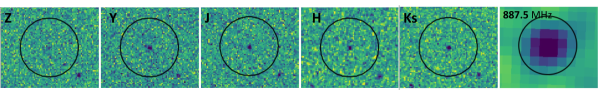
Figure 2: VIKING bands of a Z dropout at $z\sim 7$ taken from our final sample. The size of the cutouts is $\sim 25\arcsec\times 20\arcsec$ and the circle is of radius $\sim 8\arcsec$ which represents the apparent size of the ASKAP detected radio source.

Simulations of forthcoming radio surveys estimated the source count of radio emitters as a function of redshift (Bonaldi et al., 2019; Wilman et al., 2008) and it predicts hundreds of thousands of radio sources beyond $z\sim 4$. Although radio emitters such as radio-loud AGNs, Starbursts, Star-forming Galaxies (SFG)s and radio-quiet AGNs contribute to this total radio-source count, simulations demonstrate that $z\geq 4$ sky is dominated by radio-AGNs (see (Raccanelli et al., 2012, Figure 2)). Currently, $\sim$112 published radio-AGNs are known at redshift $z\gtrsim 4$ (listed in Appendix, Table A.1). This number thus indicates that the known radio source population at $z\gtrsim 4$ represents a small fraction of the total radio source population.

In some cases, it is unclear whether a detected high-redshift radio source is a radio galaxy, blazar, quasar, etc., and so we adopt the neutral term “ High redshift radio source (HzRS)” to describe any radio source detected at high redshift ($z\geq 4$) .

The mismatch between models and data indicates that known HzRS are only the tip of the iceberg. The dearth of radio sources at high redshift can be attributed to the following factors: (i) many HzRS are probably in existing radio catalogues but their redshifts have not been measured due to their faintness at optical/IR wavelengths, and (ii) previous radio surveys were not sensitive enough to detect faint HzRS

Since the ultimate goal of this series of papers is to establish the HzRS count and thus test the simulations (Bonaldi et al., 2019; Wilman et al., 2008), we expect that some missing HzRS are already in the literature, but are not classified as high-redshift radio sources. We demonstrate this by visually cross-matching Sloan Digital Sky Survey (SDSS) spectroscopy (DR12, Alam et al., 2015) with the Faint Images of the Radio Sky at Twenty cm (FIRST) (Becker et al., 1995) and NRAO VLA Sky Survey (NVSS) (Condon et al., 1998) catalogues. This search resulted in a further 33 sources at $z\gtrsim 4$, listed in Appendix, Table A.2. In each case the SDSS spectrum has been checked for supporting evidence of the redshift, such as a Lyman break or other spectral features. We note that a further list of candidates is available in the MILLIQUAS (Flesch, 2021) catalogue, but to the best of our knowledge the spectroscopy has not been checked and so that list may include some spurious candidates.

Evolutionary Map of the Universe (EMU) is one of the deepest and the largest forthcoming radio continuum surveys (Norris et al., 2011a), to be delivered by the ASKAP telescope (Johnston et al., 2007). The EMU project started with a series of Early Science observations, followed by the EMU Pilot Survey (PS; Norris et al., 2021). In this paper, we use the EMU Early Science Observations of the GAMA23 field (hereafter referred to as “G23”), which is one of the Galaxy And Mass Assembly (GAMA) survey fields (Driver et al., 2008).

Motivated by the challenge of finding missing HzRS, we make use of a search technique different from conventional radio based techniques, the Lyman Dropout technique ( a.k.a. Lyman Break Galaxy technique), to identify potential HzRS at $z\gtrsim 4-7$ in the G23 field. The Lyman dropout technique has been a popular technique in optical astronomy over the past two decades for discovering high-redshift galaxies up to $z\sim 11$. However, only one radio galaxy at $z=4.72$ has been identified using the Lyman dropout technique to date (Yamashita et al., 2020). Therefore, the primary goal of this study is to test the efficiency of Lyman dropout technique in finding HzRS. A second goal is to determine the properties of our sample of HzRS, a detailed study of which will be discussed in a future paper.

The Lyman dropout technique looks for the redshifted spectral signature of the Lyman limit at 91.2 nm (Far-UV regime). This is the longest wavelength of light that can ionise a ground-state hydrogen atom. Light at wavelengths shorter than 91.2 nm (ie. at higher energies) will be absorbed by sufficiently optically-thick atomic hydrogen present in the galaxy or its circumgalactic medium. This missing radiation creates a break in the observed spectrum. For high-$z$ galaxies, the Lyman break gets redshifted into the optical region, and can be identified using images taken in multiple filters.

The structure of this paper is as follows. In Section 2 we describe how we select HzRS in GAMA23 field from the ASKAP 887.5 MHz radio catalogue using 8-band ugriZYJK_s KiDS/VIKING photometry. In Section 3, we present our sample of HzRS candidates selected at $z\sim 4$, 5, 6, and 7. In Section 4 we present the analysis of radio and IR properties of our sample. Finally, we summarise our results in Section 5.

This study adopts a $\Lambda$CDM cosmology with $\Omega\textsubscript{m}=0.3$, $\Omega\textsubscript{$\Lambda$}=0.7$ and $H_{0}=70~{}$km s^-1Mpc^-1.

2 Data and Methods

To find HzRS, we cross-match the G23 radio observations with the Kilo Degree Survey optical catalogue (KiDS; Kuijken et al., 2019) and the VIKING DR5 & CATWISE2020 (Marocco et al., 2021) infrared catalogues. This results in a sample of G23 radio sources with optical and infrared photometry. We then apply the redshift specific Lyman dropout colour cuts (Ono et al., 2018; Venemans et al., 2013) to select the radio source candidates at $z\gtrsim 4$ in the G23 field. This paper is the first in a series describing our search for HzRS using the Lyman dropout technique as part of the EMU survey.

We use the 887.5 MHz radio continuum data of the G23 field, produced by ASKAP as part of the EMU Early Science program in early 2019. ASKAP consists of 36 antennas, each of which is equipped with a Phased Array Feed (PAF). It operates in a frequency range from 700 to 1800 MHz. ASKAP data products have been created using the ASKAPsoft pipeline, aided by Selavy software in source extraction. This study examined the following ASKAP catalogues from project AS034: (i) selavy-image.i.SB8132.cont.taylor.0.restored.components and (ii) selavy-image.i.SB8137.cont.taylor.0.restored.components, retrieved from the CSIRO Data Access portal . The observational parameters of G23-ASKAP data are given in Table 1.

A total of 38 080 radio sources are present in these 2 catalogues, of which 2107 are complex or multi-component (number of components $\geq 2$). In this paper, we focus on simple (or single component) radio sources only, which are fitted by a single Gaussian.

For the selection of $z\geq 4-6$ radio sources, we used optical data from the complementary Kilo Degree Survey (KiDS, Kuijken et al., 2019), in particular we exploited the KiDS DR4.1 multiband source catalogue, featuring Gaussian Aperture and PSF photometry ( GAaP ; see Kuijken et al. (2015) for details) measurements of KiDS-$ugri$ and VIKING-ZYJHK bands for $r$-band detected sources.

To select $z\sim 7$ radio sources, we utilized VIKING photometry in the DR5 catalog obtained from the VISTA archive. We converted the Vega magnitudes in the VIKING DR5 catalog to AB magnitudes using the Cambridge Astronomical Survey Unit (CASU) recommendations .

The mid-IR (MIR) data used in this paper comes from the Wide-field Infrared Survey Explorer (WISE, Wright et al., 2010), which is an all-sky survey centred at 3.4, 4.6, 12, and 22 $\mu$m (referred to as bands W1, W2, W3 and W4), with an angular resolution of 6.1, 6.4, 6.5, and 12.0 arcsec respectively, and typical 5$\sigma$ sensitivity levels of 0.08, 0.11, 1, and 6 mJy/beam. Here, we use data from the CATWISE2020 (Marocco et al., 2021) catalogue.

Far-IR (FIR) observations in the G23 field come from the Herschel space observatory. Herschel carried out observations using two photometric instruments on board, (i) Photodetecting Array Camera and Spectrometer (PACS, Poglitsch et al. (2010) ) and (ii) Spectral and Photometric Imaging Receiver (SPIRE, Griffin et al. (2010) ). PACS observations centred at 70 $\mu$m, 100 $\mu$m, and 160 $\mu$m mainly trace the rest-frame mid-IR emission of the high-$z$ ($z>2$) AGN. SPIRE observed simultaneously in three wavebands centred at 250 $\mu$m, 350 $\mu$m, and 500 $\mu$m, picking up the starburst emission in high-$z$ AGNs (Hatziminaoglou et al., 2010). Herschel ceased operation on 29^th April 2013 when the telescope ran out of liquid helium, which is essential for cooling the instruments. This study utilized the SPIRE (Schulz et al., 2017) and PACS point source catalogues (Marton et al., 2017) available in Infrared Science Archive (IRSA).

Table 1: Summary of G23-ASKAP survey.

Parameters	G23-ASKAP
Frequency (MHz)	887.5
Bandwidth (MHz)	288
Synth. beam size ($\arcsec$)	10
RMS ($\mu$Jy/beam)	38
Survey area (deg2)	50
Astrometric accuracy ($\arcsec$)	$\sim$ 1

2.1 Finding optical and infrared counterparts

To find the optical counterparts of radio sources, we use a simple nearest-neighbour technique. We need to choose a search radius that maximises the number of cross-matches while minimising the number of false identifications (hereafter called false-IDs). We achieve this by cross-correlating the ASKAP radio catalogue with the KiDS DR4.1 multiband optical (ugri) $+$ NIR (ZYJHK_s) photometry at a range of search radii, measuring the number of cross-matches at each radius. We then estimate the false-ID rate by shifting the radio position by 1 arcmin (so that all matches are spurious) and repeating the cross-match at the same set of radii. The false-ID rate is calculated by dividing the number of shifted cross-matches by the number of unshifted cross-matches. The result is shown in Table 2. Based on this, we have chosen 2 arcsec as the optimal search radius for this study, corresponding to a false-ID rate of 14.64% and a total cross-match rate of 63.9%. We reject sources that had multiple matches within 2 arcsec. This reduces the final number of radio-optical cross-matches to 17 447.

We followed the same procedure to select infrared counterparts to our radio sources. We cross-matched the optical (KiDS) positions of our sample with the CATWISE2020 catalog at a search radius of 2$\arcsec$. This gives a false id rate of 11.9%.

Table 2: False-ID rate estimated for ASKAP-KiDS cross-match as a function of separation radius, using the single-component source list.

Match Radius	No. of Matches	No. of Matches	False-ID Rate
(arcsec)	(unshifted)	(1 arcmin offset)	(%)
1	14 067	833	5.92
2	23 002	3 368	14.64
3	29 350	7 592	25.87
4	36 417	13 410	36.82
5	44 884	20 821	46.39

2.2 Selection of radio sources at $z\gtrsim$ 4 – 6

The Lyman dropout technique relies on finding the wavelength or passband at which the Lyman break is detected, which in turn tells us the redshift of the source, given that rest-frame wavelength of Lyman limit is 91.2 nm. For example, the Lyman break of a galaxy at $z=4$ will be observed at wavelength 4560 Å  and hence can be imaged in g-band. Similarly, for higher redshift objects, the Lyman break moves into the $r$ or $i$ or $Z$ bands.

2.2.1 Applying g, r, & i-band dropout technique

Table 3: KiDS & VIKING filters, their central wavelength, and their mean 5$\sigma$ limiting magnitude.

Filters	$\lambda$	5$\sigma$ Mag. Lim.
	(Å)	(AB)
$u$	3 550	24.23
$g$	4 775	25.12
$r$	6 230	25.02
$i$	7 630	23.68
Z	8 770	23.1
Y	10 200	22.3
J	12 520	22.1
H	16 450	21.5
Ks	21 470	21.2

Table 4: The criteria used to identify Lyman dropouts at $z\sim$ 4, 5, 6, adopted from Ono et al. (2018) and at $z\sim$ 7, taken from Venemans et al. (2013). The last row is based on our COSMOS tests, to remove low-z interlopers in $z\sim$ 4, 5, 6 sample, as described in subsection 2.2.2.

$z\sim 4$ (g dropouts)	$z\sim 5$ (r dropouts)		$z\sim 6$ (i dropouts)	$z\sim 7$ (Z dropouts)
	criteria I a	criteria II b
S/N(i) $>$5	S/N(z) $>$5	S/N(z) $>$5	S/N(z) $>$5	S/N(Y) $>$7
	S/N(g) $<$2	S/N(g) $<$2	S/N(g) $<$2 ; S/N(r) $<$2	Z-Y $\geq$ 1.1
g-r $>$ 1.0	r-i $>$ 1.2	r-i $>$ 1.0	i-z $>$ 1.5	– 0.5 $<$ Y - J $\leq$ 0.5
r-i $<$ 1.0	i-z $<$ 0.7	i-z $<$ 0.5	z-Y $<$ 0.5	Z - Y $>$ Y - J + 0.7
g-r $>$1.5 (r-i) + 0.8	r-i $>$1.5(i-Z) + 0.8	r-i $>$1.5(i-Z) + 0.8	i-z $>$2.0 (z-Y) + 1.1	-0.5 $<$ Y - K $<$ 1.0
$i_{AB}>22.2$	$z_{AB}>23$	$z_{AB}>23$	$z_{AB}>22$	J - K $<$ 0.8
				undetected in ugri bands if available

• Ono et al. (2018)

• Our relaxed r dropout criteria (see text for details.)

To find HzRS, we adopt the dropout criteria of Ono et al. (2018), shown in Table 4. The spectroscopically confirmed redshift ranges covered by each dropout, adopted from Ono et al. (2018, Figure 6), are as follows: (i) g-dropout: $3\leq z\leq 4.5$ (ii) r-dropout: $4.3\leq z\leq 5.4$ (iii) i-dropout: $5.6\leq z\leq 6.2$. To keep it simple, we use redshifts, $z\sim 4$, 5 and 6 to represent $g$, $r$, and $i$-band dropouts respectively. We use photometry from the KiDS DR4.1 multi-band catalogue (shown in Table 3), based on the GAaP magnitudes corrected for both zero-point and Galactic extinction. The 5$\sigma$ limiting magnitude for the $g$-band was used in the $g-r$ colour if objects were undetected ( i.e. no entry in the catalogue) in $g$-band. Similarly, a 5$\sigma$ limiting magnitude for the $r$ and $i$-bands were used to estimate $r-i$ and $i-z$ colours for $r$ and $i$ dropouts if objects were undetected in $r$ and $i$ band respectively. In Table 5, we describe the photometric selection and number of sources remaining after applying $z\sim 4$, 5, and 6 colour cuts. We present examples for all three dropouts, taken from our final sample, in Figure 1, showing their cutouts at each of the ugriZYJHKs bands.

Ideally, the signal-to-noise-ratio (SNR) of the sources should be used to measure their detection or non-detection in a given band. Since such information is not present in the KiDS catalogue, we utilized the mean 5$\sigma$ limiting magnitude of each passband to define detection and undetection. Given that the 5$\sigma$ limiting magnitude follows a continuous distribution (Kuijken et al., 2019), this could result in some dropouts being missed.

Table 5: Our initial sample: the number of radio sources remaining after each criterion. Sources lacking detection in a given dropout (no entry in the catalog) band is replaced with their respective mean 5$\sigma$ limiting magnitude.

Sample	Criteria	Radio source
		Count
G23-ASKAP	–	35,973
	cross-match with KiDS at 2″	23 002
	After removing multiple matches	17 447
	imaflags_iso = 0 &	17 396
	nimaflags_iso = 0
	flag_gaap_$gri$ = 0	17 396
	flag_gaap_$griZ$ = 0	17 376
	col 1,Table 4 colour cuts &	229
$z\sim 4$ sample	Mag_gaap_i < 23.8 &
($g$ detected)	Mag_gaap_u > 24.23 or undetected
	col 1,Table 4 colour cuts &	6
	Mag_gaap_g = 25.12 &
$z\sim 4$ sample	Mag_gaap_i < 23.8 a  &
($g$ undetected)	Mag_gaap_u > 24.23 or undetected
	col 3,Table 4 colour cuts&	58
$z\sim 5$ sample	Mag_gaap_Z < 23.6 b  &
($r$ detected)	Mag_gaap_u > 24.23 or undetected &
	Mag_gaap_g > 25.12 or undetected
	col 4,Table 4 colour cuts &	6
$z\sim 6$ sample	Mag_gaap_Z < 23.6b  &
($i$ detected)	Mag_gaap_u > 24.23 or undetected
	Mag_gaap_g > 25.12 or undetected
	Mag_gaap_r > 23.68 or undetected
	col 4,Table 4 colour cuts &	9
$z\sim 6$ sample	Mag_gaap_Z < 23.6b  &
($i$ undetected)	Mag_gaap_u > 24.23 or undetected
	Mag_gaap_g > 25.12 or undetected
	Mag_gaap_r > 23.68 or undetected

• $i$-band $5\sigma$ limiting magnitude (AB) correspond to the end of the peak of the distribution (Kuijken et al., 2019, Figure 3).

• $Z$ band $5\sigma$ limiting magnitude (AB) distribution correspond to the end of the peak of the distribution, assuming a spread of $\pm 0.5\sigma$, given that the nominal $5\sigma$ $Z_{lim}=23.1$.

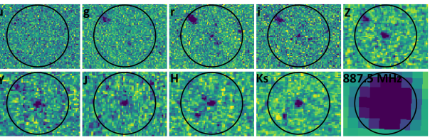
(a) An example of g dropout at $z\sim 4$ taken from our final sample: J223541-311145. The size of the cutouts is $\sim 20\arcsec\times 15\arcsec$ and the circle is of radius $\sim 7.4\arcsec$ which represents the apparent size of the ASKAP detected radio source.

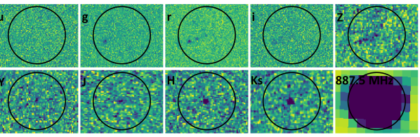
(b) An example of r dropout at $z\sim 5$ taken from our final sample: J230551-343338. The size of the cutouts is $\sim 24\arcsec\times 18\arcsec$ and the circle is of radius $\sim 8\arcsec$ which represents the apparent size of the ASKAP detected radio source.

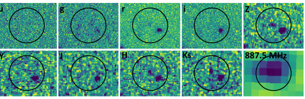
(c) An example of i dropout at $z\sim 6$ taken from our final sample: J230246-293923. The size of the cutouts is $\sim 20\arcsec\times 15\arcsec$ and the circle is of radius $\sim 6\arcsec$ which represents the apparent size of the ASKAP detected radio source.

Figure 1: KiDS-ugri and ViKING-ZYJHKs images of Lyman dropouts at each redshift are illustrated above in the order of increasing wavelength. The Lyman break can be identified by combining photometry in three consecutive bands. At $z\sim 4$, the Lyman limit ($\lambda\textsubscript{rest}=912\textup{\AA}$) falls in the g-band and shorter wavelengths are significantly absorbed, as indicated by faint $u$ and $g$ bands. Similarly for $z\sim 5$ and 6 sources, the Lyman limit falls in the $r$ and $i$-bands respectively.

2.2.2 Removing low-$z$ interlopers from our $z\gtrsim 4-6$ sample

Low-$z$ objects such as dwarf stars and passive galaxies can enter the selection region defined by Lyman dropout colour cuts due to photometric errors, even though intrinsically they do not enter the colour selection window. We evaluate the contamination rate in the $z\sim 4$, 5 and 6 selection window by testing the Lyman dropout technique on a set of objects with known spectroscopic redshifts. We chose the COSMOS field (Scoville et al., 2007), a well-studied region of the sky where both broadband optical photometry and spectroscopic redshifts are available. We used the following catalogues of the COSMOS field, available in the public IRSA domain, to test $g$, and $r\&$ $i$-band dropout techniques respectively ; (i) COSMOS Photometry Catalogue January 2006 (hereafter, COSMOS2006 catalog; Capak et al. (2007)) and (ii) COSMOS2015 Catalog (Laigle et al., 2016). The spectroscopy for COSMOS sources was obtained from COSMOS DEIMOS Catalogue (Hasinger et al., 2018). We utilized the Subaru-griz photometry in the COSMOS catalogues to test the colour cuts. Furthermore, in this paper, we follow lowercase and uppercase notation in the literature for the Subaru z filter and the VIKING Z filter respectively.

We crossmatched the COSMOS 2006 catalogue and the COSMOS DEIMOS Catalogue at 1″, resulting in 8906 matches. We further excluded multiple matches and apply the following criteria as recommended in Capak et al. (2007) to obtain a cleanest sample: blend$\_$mask = 0, i$\_$mask = 0, b$\_$mask = 0, and v$\_$mask = 0. This results in 6 787 unique sources that have been deblended and are without any photometric flags to test the $g$-band dropout colour cuts. We further corrected the $g$, $r$, and $i$ magnitudes for Galactic extinction following the recommendations in Capak et al. (2007).

Similarly, we crossmatched the COSMOS2015 catalogue and the COSMOS DEIMOS Catalogue at 1″, resulting 7640 matches. The sources with multiple matches were excluded and the following criteria were applied as per Laigle et al. (2016): $flag\_HJMCC=0\&flag\_cosmos=1\&flag\_peter=0$, giving a source count of 7 502. We finally applied respective Galactic extinction corrections to $r$, $i$, $z$, and $Y$ bands as per Laigle et al. (2016).

Table 4 shows that $z\sim 4$, 5, and 6 galaxy candidates can be selected based on their gri, riz, izy colours respectively. We demonstrate this in Figure 3 by plotting the spectroscopic redshift distribution of COSMOS sources in g$-$r vs. r$-$i, r$-$i vs. i$-$z and i$-$z vs. z$-$Y colour-colour space. To test the $z\sim 7$ or Z-band dropout colour cuts, deep spectroscopic data ($z_{spec}>6.4$) is needed, which is not available in the COSMOS DEIMOS catalog. It is evident that the photometric selection window of g-dropouts (the black box) encompasses almost all $z\sim 4$ sources, with a small contribution from low-$z$ “interloper” sources. By contrast, the r-dropout selection window misses a significant fraction of $z\sim 5$ sources. Therefore, we relaxed the $r$ dropout colour cuts as follows:

$$r-i>1.0;\\ i-z<0.75;\\ r-i>1.5*(i-z)+0.8$$ (1)

The resulting colour locus is indicated by black dashed lines, showing that more $z\sim 5$ sources get included than low-$z$ ones.

In Figure 4, we demonstrate that $g$ and $r$ dropouts suffer significant contamination from low-$z$ sources at the bright end. Based on this, we introduce further selection criteria in the form of a magnitude cut-off in $i$-band (i_AB $>$ 22.2) for $g$-dropouts and in $z$-band (z_AB $>$ 23) for $r$-dropouts, which helps to reduce the contribution from low-z sources (see bottom row of Table 4).

We further note that our sample size of $i$-band dropouts is too small to draw any conclusion. The $Z$ band magnitude cut-off ($Z_{AB}>24$) implied by the figure 4 is too high and the VIKING data is also not deep enough to apply this cut-off. Therefore, we performed a literature search to to find the $Z$-band magnitude of known $z\sim 6$ quasars. Based on the spectroscopically confirmed $i$ - band dropouts in Venemans et al. (2015, Table 3), we applied a magnitude cut-off, Z_AB $>$ 22 for $i$-dropouts.

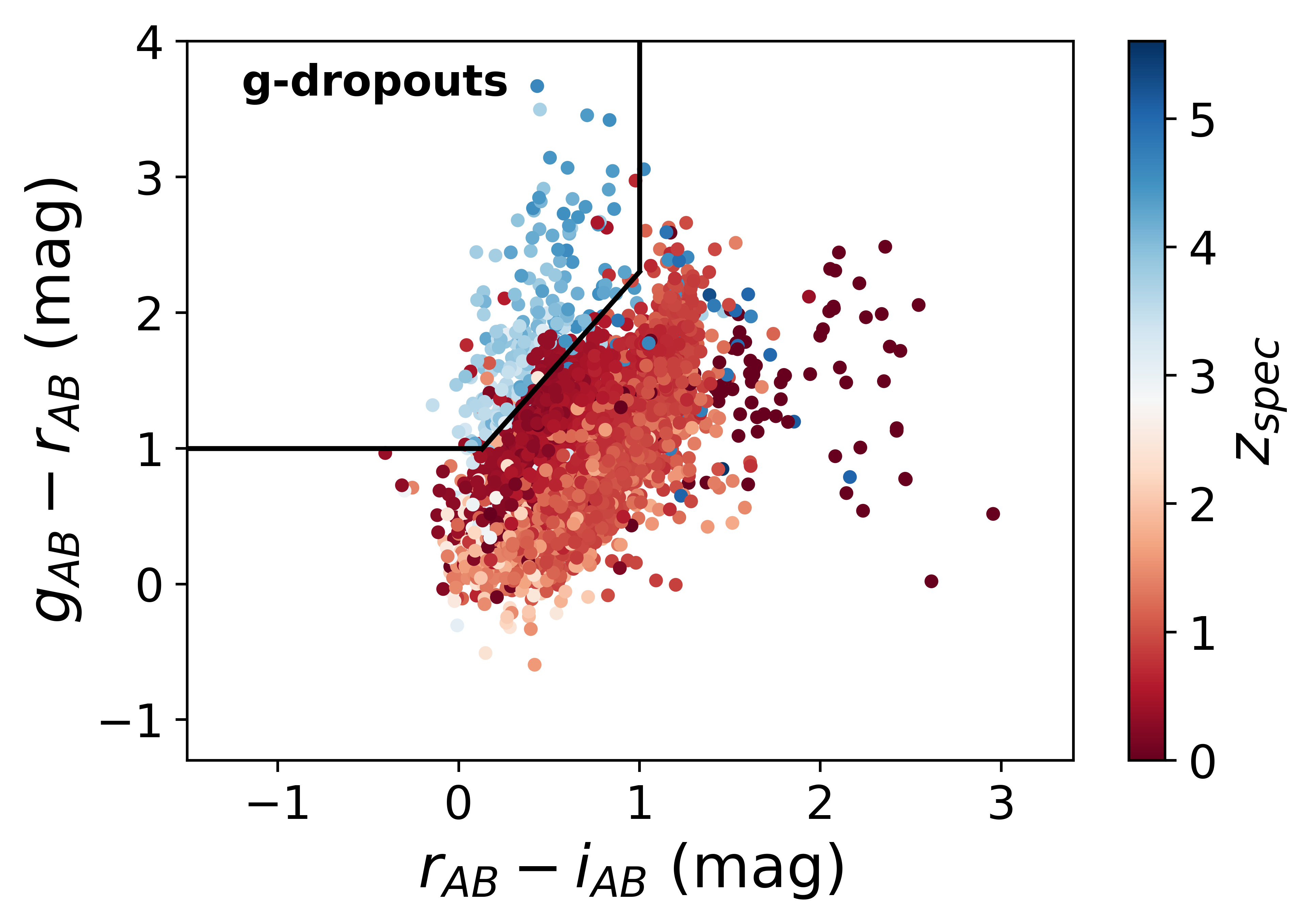
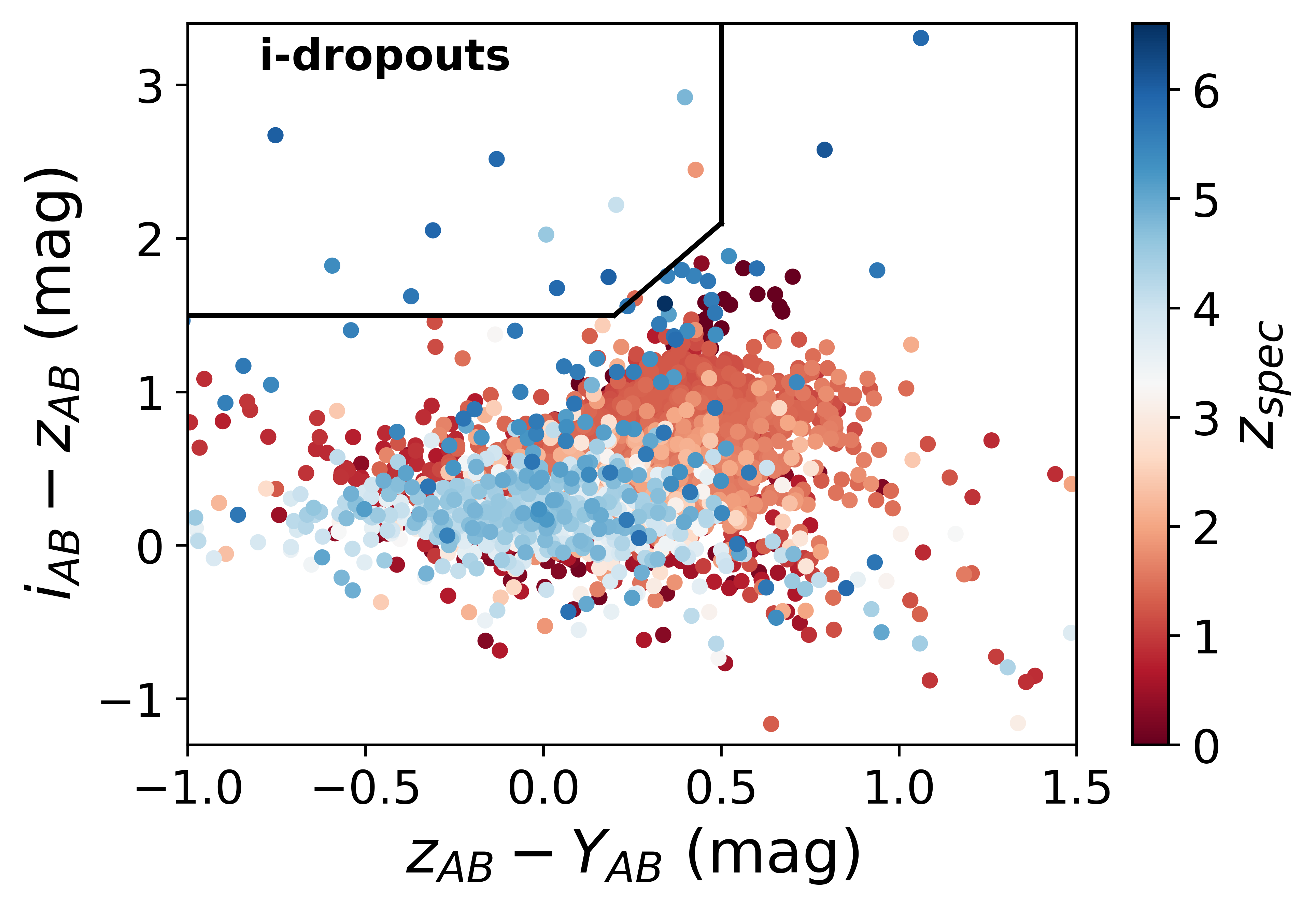
Figure 3: (Top Left) Selection of $z\sim 4$ sources by means of $g$-band dropout technique using $gri$ broadband filters: (g-r) vs. (r-i) colour-colour diagram of COSMOS sources, colour coded according to their spectroscopic redshift. The black box represents the $g$ dropout selection criteria in Ono et al. (2018). It encompasses almost all $z\sim 4$ sources, but with a small contamination from low-$z$ sources too. (Top Right) Selection of $z\sim 5$ sources by means of $r$-band dropout technique using $riz$ broadband filters: (r-i) vs. (i-z) colour-colour diagram of COSMOS sources, colour coded according to their spectroscopic redshift. The black box (solid lines) represents the $r$ dropout selection criteria in Ono et al. (2018). The black box bordered by dashed black lines represent the colour locus from relaxed $r$ band colour-cuts. (Bottom) Selection of $z\sim 6$ sources by means of $i$-band dropout technique using $izY$ broadband filters: (i-z) vs. (z-Y) colour-colour diagram of COSMOS sources, colour coded according to their spectroscopic redshift. The black box represents the $i$ dropout selection criteria in Ono et al. (2018).

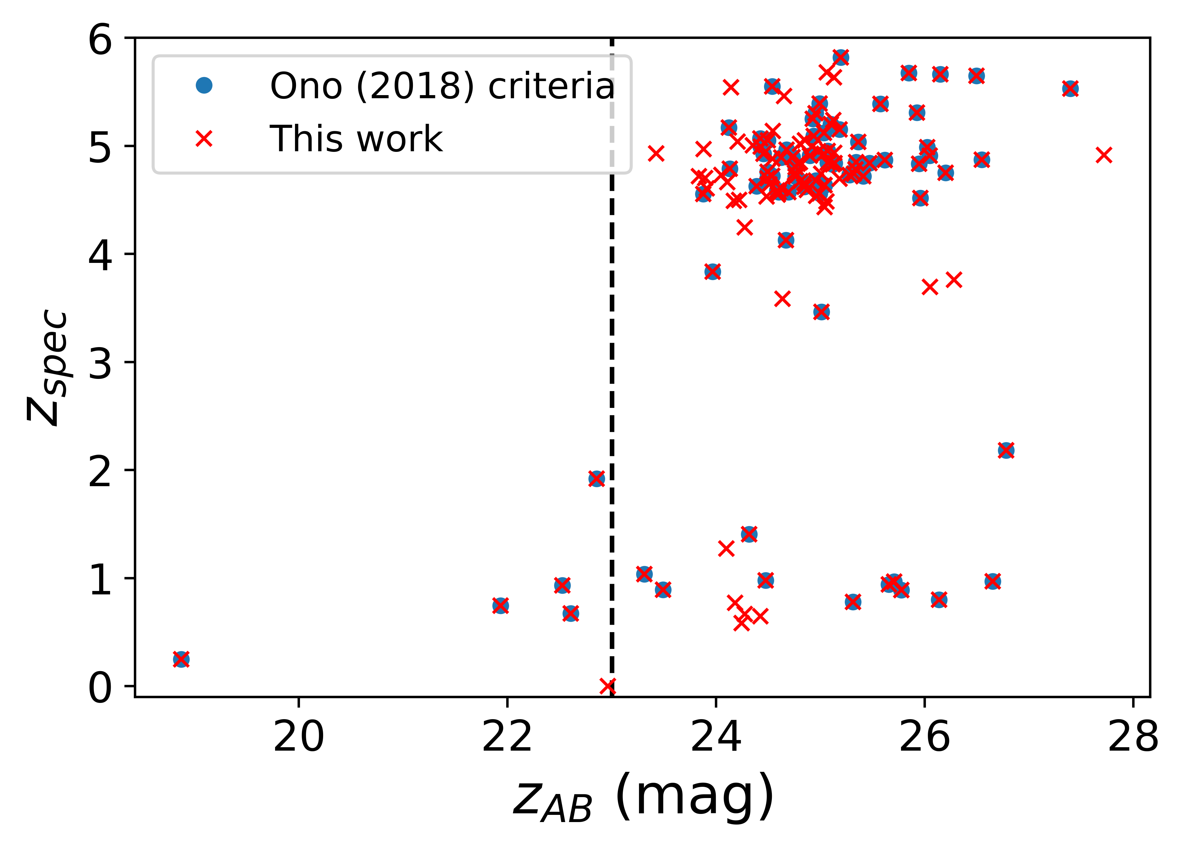
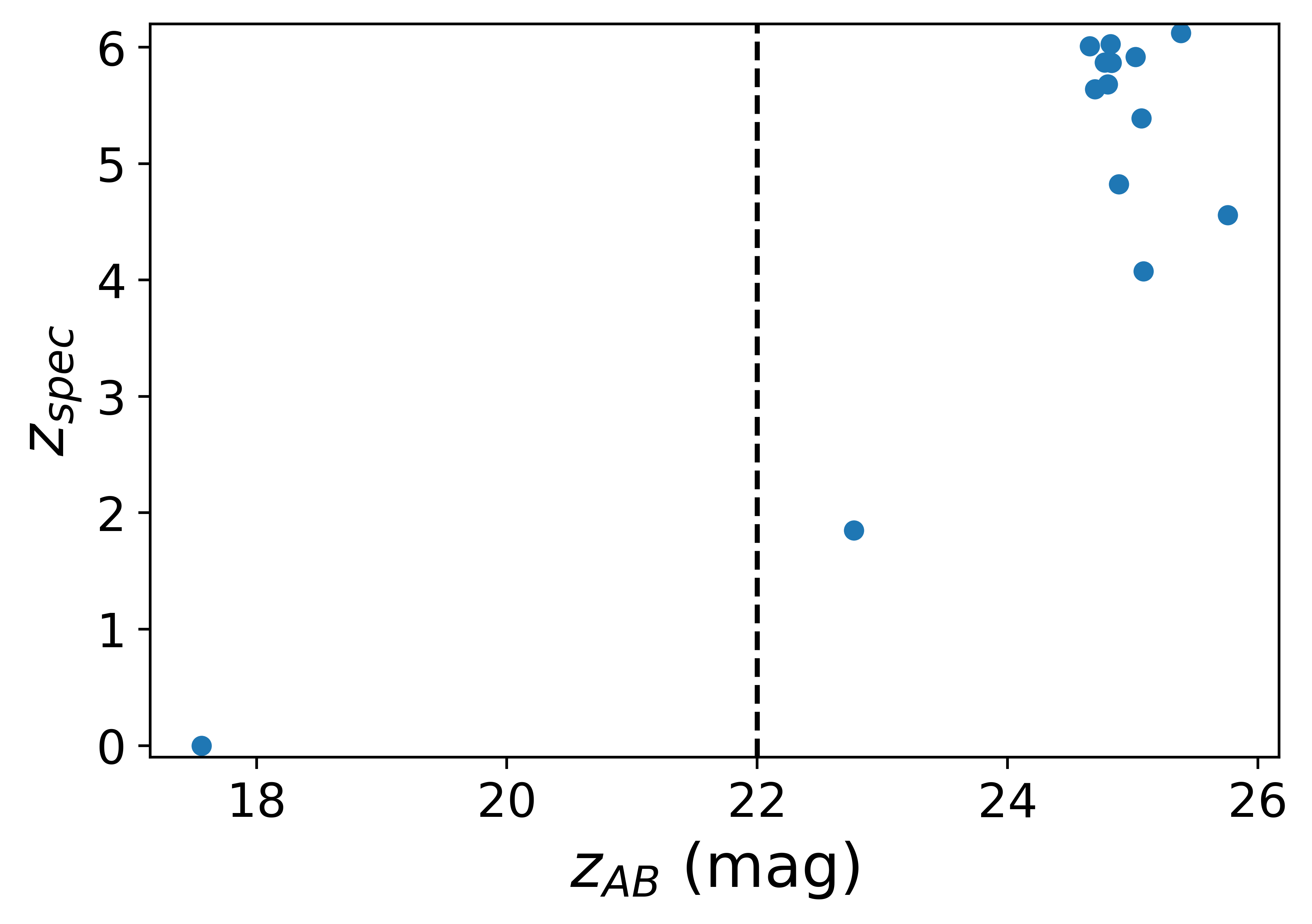
Figure 4: Selecting low-$z$ interlopers in $g$ and $r$ dropout samples in COSMOS field by utilising the respective detection bands of each dropout: (Top Left) $i$ magnitude of $g$ dropouts together with their spectroscopic redshifts. (Top Right) $z$ magnitude of $r$ dropouts together with their spectroscopic redshifts. Blue solid circles represent the $r$ dropouts selected using Ono et al. (2018) criteria and red crosses, the $r$ dropouts selected using our relaxed colour-cuts (Equation 1). (Bottom:) $z$ magnitude of $i$ dropouts together with their spectroscopic redshifts.

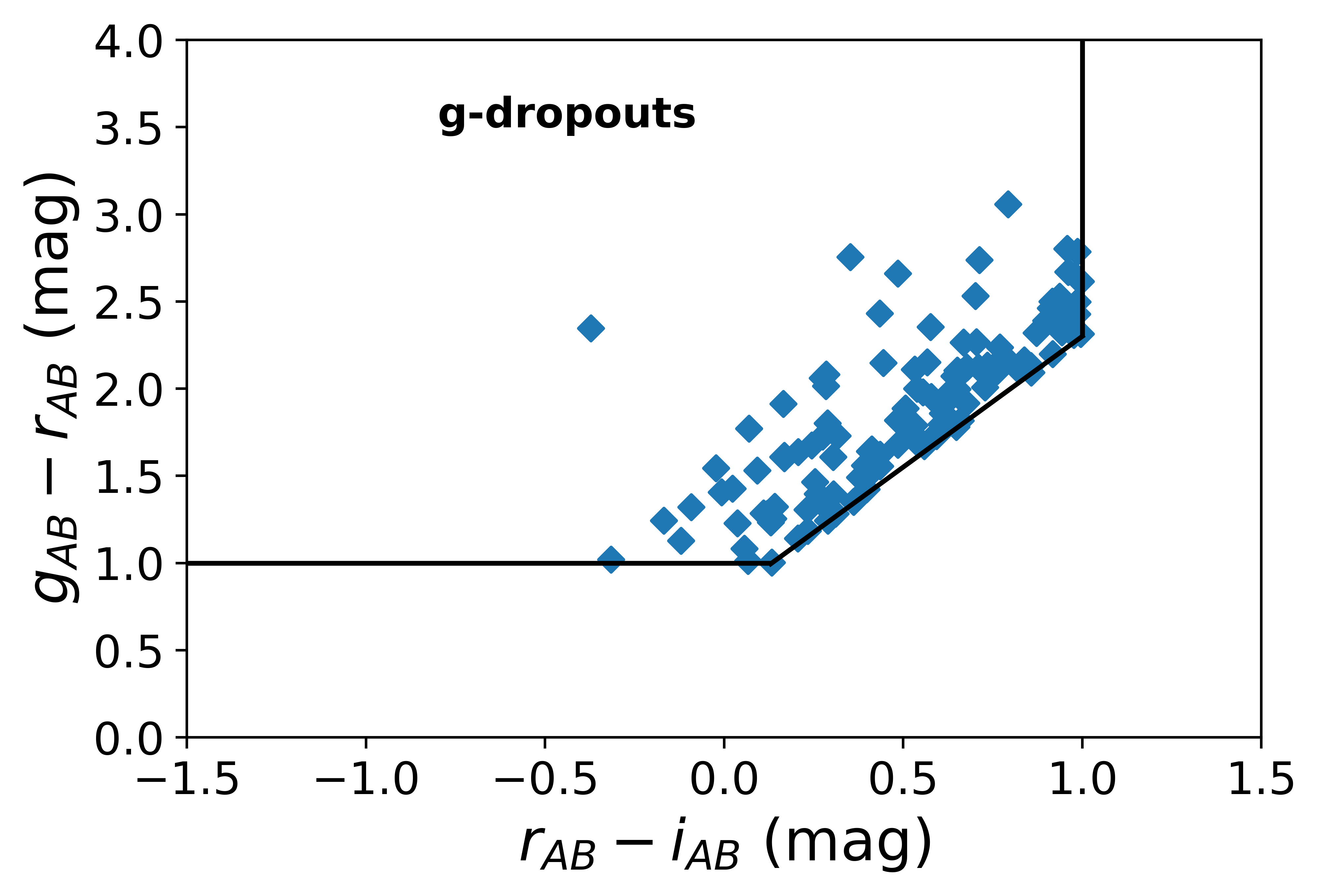
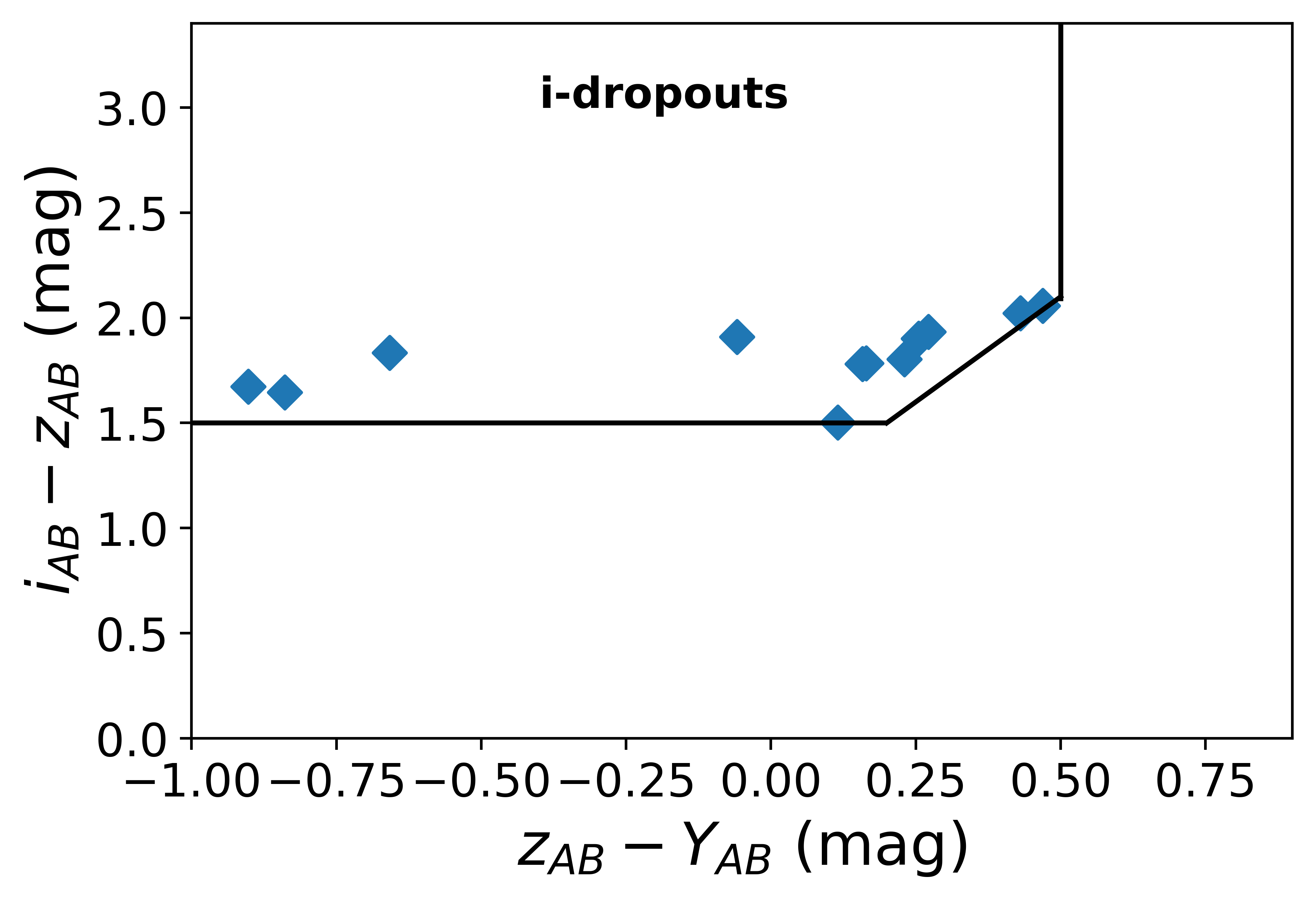
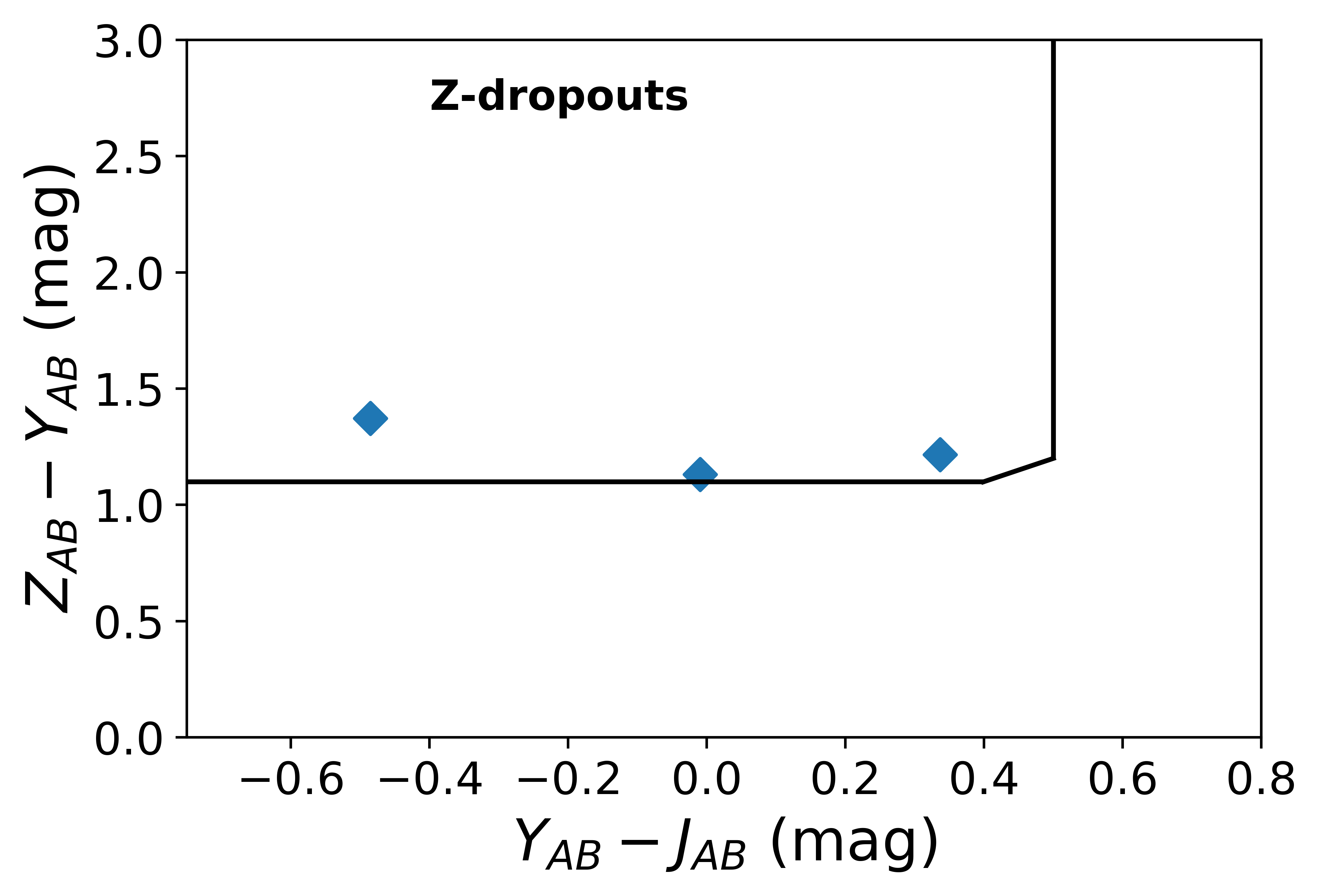
Figure 5: Colour-colour diagram of our final sample of HzRS at $z\gtrsim$4-7 selected via the Lyman dropout technique. The black box shows the selection criteria of $g$, $r$, $i$, and $Z$ dropouts in $gir$, $riZ$, $iZY$, and $ZYJ$ colour-colour plane respectively.

2.3 Selection of radio sources at $z\sim 7$

We utilised VIKING photometry to search for radio sources in the redshift range, $6.44\leq z\leq 7.44$. Venemans et al. (2013) demonstrated that Lyman dropouts at $z\sim 7$ (a.k.a Z dropouts) can be selected using ZYJ near-IR filters. We cross-matched G23-ASKAP radio catalogue and VIKING DR5 catalogue at a search radius of 2$\arcsec$, which gives a false ID rate of 7.9% . Using the selection method in Venemans et al. (2013) (see Table 4), we select a sample of 3 radio source candidates at $z\sim 7$, of which one is a known radio-quasar, VIK J2318-3113, at $z=6.44$ (Ighina et al., 2021). Scattering of foreground galaxies into the Z-dropout selection region in the ZYJ color-color space is minimised by selecting point sources only by applying the criterion: pGalaxy$<0.95$ ( see Venemans et al. (2013) and reference therein for details), where pGalaxy is the probability that the source is a galaxy.

2.4 Estimate of Reliability

Finally, we estimate the success rate of our magnitude cutoff by counting the fraction of low-$z$ sources remaining after applying the $i$-band and $z$-band cutoff to $g$ and $r$ & $i$ dropouts respectively. A sample of 294 sources were identified from the COSMOS catalog as satisfying the $z\sim 4$ colour cuts (Table 4), of which 75 sources have $z_{\textrm{spec}}$ below 3.0, resulting in a contamination rate of 25.5%. The further application of the i_AB $>$ 22.2 criterion reduces the low-z source count to 29 and the total sample size to 248. This gives a final contamination rate of 11.7%.

A total of 78 sources were identified as $r$ dropouts using Ono et al. (2018) criteria, of which 19 have $z_{\textrm{spec}}<4.3$ giving a contamination rate of $\sim 24.4\%$. On the other hand, relaxed $r$ band colour cuts (Equation 1) selected 127 sources in total, of which 29 have $z_{\textrm{spec}}<4.3$ resulting a contamination rate of $\sim 22.8\%$. This shows that relaxed $r$ band colour cuts select $\sim 1.7$ times more $z_{\textrm{spec}}>4.3$ sources than the Ono et al. (2018) criteria while the contamination rate remains almost constant. We further reduce the contamination rate to 19% by applying a z_AB $>$ 23 cutoff.

Due to the dearth of deep spectroscopic data, only 14 sources were selected as $i$ dropouts, 6 of which have a $z_{\textrm{spec}}<5.6$ classifying as interlopers. This gives an initial contaminant rate of $\sim 43\%$ and the further application of magnitude cut-off, $Z_{AB}>22$, results a final contaminants rate of $\sim 38.4\%$.

This shows that the $z\sim 4$ sample is $\sim 88\%$ reliable while the $z\sim 5$ sample is around 81% reliable. The $z\sim 6$ sample is $\sim 62\%$ reliable, which is likely to be a lower limit given that the sample size was smaller. There is no robust way of estimating the reliability for the $z\sim 7$ sample, as there is a lack of deep spectroscopic data in COSMOS.

We applied these magnitude cut-offs to the sources in Table 5 to select our final sample of radio source candidates at $z\gtrsim 4-6$ in the G23-ASKAP field. The resulting source count of each dropout is shown in Table 6. As a further check on reliability, we cross-matched our sample with the GAMA spectroscopic redshift (Baldry et al., 2018) catalogue and the Gaia Early Data Release 3 (EDR3, Brown et al., 2020). The Gaia satellite measures parallaxes and proper motions for nearby stars in our Milky Way, and allow us to identify cool dwarf stars, if any, in our final sample. Gaia EDR3 is the latest release, providing information for about 1.8 billion objects.

None of our sources were found to have either GAMA spectroscopic or GAIA counterparts out to a search radius of 4 arcsec. The lack of GAMA spectroscopic counterparts is consistent with a high redshift, as the GAMA spectroscopic survey is complete to $z\sim 0.4$. Similarly, the lack of GAIA counterparts confirms that (i) no Milky Way stars are present in our sample, and (ii) no low-z quasars that are bright enough to be detected by GAIA are in our final sample.

3 Results

Using the Lyman Dropout photometric technique and our additional magnitude cut-offs (Table 4) to reduce low-$z$ interlopers, we select our final sample of 148 radio source candidates at $z\gtrsim 4-7$, where (i) g & i dropouts criteria come from Ono et al. (2018) (ii) r dropout criteria from this study (Equation 1) and (iii) Z dropout criteria from Venemans et al. (2013).

The colour-colour plot of our final sample is shown in Figure 5. Furthermore, we identify a known radio quasar at $z=6.44$ and 2 radio source candidates at $z\sim 7$ using the Z-dropout selection technique from Venemans et al. (2013). Thus our final sample of 149 radio sources in 50 deg² implies a sky density of $\sim 3$ per $deg^{2}$ for $S_{888}\gtrsim 0.1$ mJy radio sources at $z\gtrsim 4$. For comparison, Norris et al. (2021) suggested a sky density of $\sim 5$ per $deg^{2}$ beyond $z\sim 4$ at EMU flux limit, based on simulations. We present the catalogues of $z\gtrsim 4-6$ and $z\sim 7$ sources, including KiDS/VIKING and WISE W1 photometry, in Table LABEL:tab:catalog and Table 8 respectively.

Table 6: Our final sample of $z\gtrsim 4-7$ candidates in G23 field selected using Lyman dropout colour cuts (Table 4) together with our magnitude cutoffs from Figure 4

. Redshift ($z$) Sample Size $z\sim 4$ 117 $z\sim 5$ 14 $z\sim 6$ 15 $z\sim 7$ 3

Table 7: Our final $z\gtrsim 4-6$ sample, showing radio properties from ASKAP and optical/ IR photometry from KiDS and CATWISE catalogues respectively. Missing optical magnitudes indicate non-detection in that respective filter. The missing WISE magnitude (W1) indicate no counterpart within 2 arcsec of the KiDS position. KiDS/VIKING magnitudes are given in the AB system and the WISE magnitudes in the Vega unit.

Index	ASKAP	RA	DEC	S887.5	Mag_u	Mag_g	Mag_r	Mag_i	Mag_Z	W1
	name	(deg)	(deg)	(mJy)						(mag)
$z\sim 4$ Sample ($g$ dropouts)
1	J225745-311209	344.437	-31.203	0.32	25.067	25.779	24.108	23.549	22.928
2	J225802-345205	344.511	-34.868	0.948		25.954	23.293	22.808	21.720	17.588
3	J225835-325509	344.649	-32.919	0.237		25.220	23.268	22.689	21.573	15.633
4	J225915-314116	344.815	-31.688	0.57		24.348	22.954	22.649	21.796	16.055
5	J230041-322125	345.172	-32.357	0.247		25.854	23.887	23.248	21.810	15.95
6	J230122-294717	345.342	-29.788	0.254	24.800	25.084	23.678	23.685	23.143
7	J230156-331615	345.484	-33.271	0.261	24.993	25.791	23.483	22.506	21.295	15.556
8	J230223-294300	345.599	-29.716	0.584	24.999	25.341	23.511	22.884	22.187	17.686
9	J230234-335010	345.645	-33.836	0.246		25.306	23.750	23.314	23.198
10	J230249-322437	345.708	-32.411	0.233		26.273	24.163	23.632	22.896	16.641
11	J230306-333335	345.778	-33.559	0.282			23.845	23.724
12	J230317-345556	345.824	-34.932	2.428		25.179	23.003	22.217	21.372	16.771
13	J230432-341722	346.133	-34.289	6.517	25.132	24.487	23.360	23.481	23.491
14	J230504-292342	346.267	-29.395	0.646		25.831	23.852	23.297	22.074	17.746
15	J230516-331612	346.317	-33.270	0.421		25.096	23.024	22.381	22.067
16	J230544-351610	346.434	-35.269	0.302		24.140	23.057	23.002	22.886
17	J230547-293327	346.449	-29.557	2.886	24.393		23.511	23.343	22.727
18	J230718-310125	346.826	-31.024	0.364		24.013	22.692	22.784	22.728
19	J230831-350015	347.133	-35.004	0.203		24.927	23.111	22.451	21.681	16.86
20	J230832-340644	347.137	-34.112	8.009	25.594	24.677	23.069	22.766	22.104	16.219
21	J230905-334318	347.272	-33.722	0.204		25.661	23.539	22.862	21.849
22	J230937-323421	347.405	-32.573	0.272		25.599	23.829	23.760	22.196	16.971
23	J230940-335143	347.418	-33.862	0.298		24.765	23.522	23.691	24.487
24	J230942-335049	347.427	-33.847	0.304			23.385	22.792	21.804	16.54
25	J231057-294135	347.740	-29.693	0.431		25.159	23.852	23.621	22.309	16.91
26	J231117-323952	347.822	-32.664	0.247		25.543	24.052	23.674	23.917
27	J231148-311231	347.950	-31.209	0.323	25.134	24.726	22.381	22.753	22.904	18.202
28	J231149-304758	347.958	-30.799	0.292	24.414	24.550	23.228	23.087	22.582	16.862
29	J231210-332436	348.045	-33.410	0.26	24.598	25.670	24.111	23.718	23.112	17.172
30	J231421-344141	348.587	-34.695	0.749	24.784	24.396	22.718	22.233	22.000	16.423
31	J231444-291949	348.684	-29.330	0.276		26.165	23.711	22.739	21.711	16.301
32	J231449-293938	348.706	-29.661	1.205	24.960	25.635	23.636	23.097	21.851	16.812
33	J231508-312105	348.784	-31.351	0.244		25.858	24.062	23.455	22.462	17.192
34	J231508-341955	348.787	-34.332	98.088		25.778	23.454	22.511	21.470	15.897
35	J231555-311458	348.979	-31.249	0.472		26.288	23.857	23.423	22.709	17.889
36	J231604-324740	349.020	-32.795	0.151		26.329	24.171	23.403	22.477	16.847
37	J231617-303200	349.073	-30.533	3.779		25.763	23.302	22.391	21.255	15.878
38	J231632-331953	349.134	-33.332	1.342	24.946	24.309	22.669	22.263	21.888	17.111
39	J231645-301948	349.189	-30.330	0.763		24.803	23.166	22.959	21.994	18.09
40	J231648-303629	349.201	-30.608	0.356		25.818	23.713	23.062	22.658	16.939
41	J231719-315344	349.332	-31.896	0.205	25.291	24.586	23.584	23.451	23.077
42	J231723-301556	349.348	-30.266	0.464		24.145	22.748	22.487	22.705	18.284
43	J231737-313228	349.407	-31.541	0.259	24.763	26.235	23.565	22.605	21.880	16.663
44	J231752-311151	349.468	-31.197	0.324		24.784	23.772	23.705	22.739	16.736
45	J231826-323746	349.610	-32.629	0.374	24.867	25.198	23.653	23.676	22.280	16.01
46	J231828-310408	349.618	-31.069	0.197		24.853	23.426	23.403	22.139	17.125
47	J231850-303818	349.708	-30.638	0.2		25.686	22.949	22.236	21.583	16.557
48	J231853-293420	349.722	-29.572	0.361	24.365	26.231	24.235	23.583	22.366	16.635
49	J232019-294205	350.081	-29.702	0.572		25.674	24.177	23.777	22.864	15.97
50	J232020-343818	350.084	-34.638	0.257		25.217	23.124	22.267	21.1660	16.308
51	J232034-305242	350.143	-30.879	0.506		26.007	23.508	22.591	21.225	16.13
52	J232043-320457	350.182	-32.083	3.006	25.217	25.887	23.793	23.129	22.256	16.822
53	J232130-320208	350.377	-32.036	0.294	25.261	24.562	23.421	23.215	21.940	17.03
54	J232135-320117	350.399	-32.022	0.266		24.778	22.919	22.309	21.839	16.359
55	J232140-311522	350.417	-31.256	0.47		25.638	23.374	22.705	21.997	17.304
56	J232246-331448	350.691	-33.247	0.277	24.752	26.199	23.584	22.589	21.546	16.676
57	J232331-345632	350.882	-34.942	0.639		26.101	23.673	22.688	21.728	15.694
58	J232338-350353	350.910	-35.065	0.988		24.471	23.451	23.767	22.534	18.065
59	J232347-344625	350.948	-34.774	0.726		25.682	23.363	22.491	21.452	15.994
60	J232413-303039	351.057	-30.511	0.457		26.281	23.783	22.797	21.864	16.669
61	J232515-295957	351.314	-29.999	1.317		24.565	22.944	22.509	22.097	17.487
62	J232515-314448	351.314	-31.747	1.431	24.848	26.250	23.447	22.489	21.277	16.122
63	J222915-334311	337.314	-33.719	1.992		25.057	23.829	23.792	23.329
64	J223018-304213	337.576	-30.704	2.954		25.314	23.629	23.089	22.573	17.405
65	J223054-322552	337.727	-32.431	75.829		25.564	23.444	22.627	21.861	17.538
66	J223215-301935	338.066	-30.327	10.809		26.243	23.488	23.135	22.872	18.29
67	J223508-295809	338.785	-29.969	1.081		24.139	22.897	22.607	22.438
68	J223531-291912	338.879	-29.320	0.744	24.549	25.323	23.572	23.050	22.325	16.968
69	J223533-343305	338.889	-34.552	1.942	24.406	24.286	23.031	22.894	21.702	17.279
70	J223541-311145	338.922	-31.196	0.689		26.473	24.012	23.065	21.906	16.757
71	J223710-305549	339.294	-30.930	2.54		25.052	23.322	23.006	22.722	16.801
72	J223729-325838	339.374	-32.977	0.337	24.749	25.078	23.796	23.485	22.158	16.236
73	J223743-333305	339.432	-33.551	1.05		24.747	23.514	23.384	22.600	16.724
74	J223831-330728	339.629	-33.124	0.249		25.445	23.981	23.727	24.024
75	J223936-295303	339.900	-29.884	2.703		25.995	23.209	22.222	21.617	16.493
76	J224017-325128	340.073	-32.858	0.398	24.662	25.188	23.179	22.451	22.441	16.653
77	J224040-295600	340.168	-29.933	2.673	24.283	24.770	22.952	22.466	20.989	16.221
78	J224047-331331	340.197	-33.225	0.646		25.308	23.958	23.689	23.193
79	J224138-331346	340.411	-33.229	0.242		25.162	23.246	22.570	21.842	17.368
80	J224145-340622	340.439	-34.106	66.186		26.2801	23.891	22.992	21.688	16.254
81	J224203-333606	340.513	-33.602	0.769	25.436	25.747	23.598	23.154	24.637	16.188
82	J224246-335928	340.692	-33.991	1.751		25.566	23.892	23.647	23.481
83	J224249-333814	340.706	-33.637	0.55		25.751	23.515	22.745	21.976	17.565
84	J224308-313622	340.784	-31.606	0.662	24.432	25.657	24.005	23.593	22.933	17.425
85	J224311-332250	340.796	-33.381	4.432		25.643	23.491	22.924	21.404	16.056
86	J224354-333900	340.976	-33.650	0.272	25.384	25.028	23.303	23.028	21.557	16.502
87	J224401-315431	341.0056	-31.909	11.74		26.160	23.101	22.309	21.1800	15.864
88	J224417-350540	341.072	-35.094	0.622	24.869	25.819	23.907	23.741	22.267	17.523
89	J224445-314547	341.188	-31.763	4.325		25.334	23.252	22.967	21.969
90	J224519-342942	341.329	-34.495	0.535		25.644	23.446	22.529	21.990	16.562
91	J224540-313747	341.418	-31.629	0.221	25.059	24.642	22.851	22.319	21.532	16.265
92	J224540-330700	341.419	-33.117	1.679	24.517	25.802	23.269	22.568	21.588	16.067
93	J224552-312733	341.468	-31.4592	0.409		26.263	23.615	22.636	22.315	16.989
94	J224601-310331	341.508	-31.059	0.685	25.250	26.278	24.116	23.278	22.031	16.936
95	J224615-285257	341.565	-28.883	1.177		24.328	22.526	22.237	22.035
96	J224623-311641	341.597	-31.278	0.206	24.845	25.129	23.845	23.735	22.802	18.402
97	J224629-323825	341.622	-32.640	0.824		25.533	23.647	23.141	22.331	16.925
98	J224630-343853	341.628	-34.648	0.599	24.742	26.381	24.066	23.071	21.513	16.402
99	J224642-311527	341.677	-31.258	0.189	24.730	25.230	23.807	23.410	22.712
100	J224710-321939	341.792	-32.328	0.476	24.249		23.011	22.249	21.336	16.425
101	J224716-310058	341.817	-31.016	0.32		26.009	23.856	23.021	21.859	17.402
102	J224812-335035	342.051	-33.843	0.36	25.272	26.052	24.037	23.753	21.790	16.874
103	J224918-314457	342.327	-31.749	4.265		25.877	23.815	23.540	24.035
104	J224955-294536	342.479	-29.760	0.294	24.707	26.023	23.892	23.036	22.479	16.346
105	J225029-350452	342.622	-35.0811	0.663		25.287	23.936	23.575	22.385	16.907
106	J225052-331301	342.719	-33.217	0.49	24.649	25.228	23.448	22.800	21.656	16.539
107	J225214-310846	343.061	-31.146	2.607		26.549	24.020	23.083	22.204	16.635
108	J225240-302302	343.166	-30.384	0.384		26.053	23.786	23.082	21.805	16.802
109	J225257-351113	343.238	-35.187	0.275	25.510	25.626	23.263	22.320	21.177	16.124
110	J225300-302322	343.253	-30.389	0.49		24.503	23.148	22.869	22.856
111	J225312-305344	343.303	-30.896	0.188	24.612	25.492	23.359	22.624	22.381	16.758
112	J225314-295139	343.311	-29.861	0.365		25.334	23.804	23.712	24.634
113	J225332-313319	343.386	-31.555	0.242	24.613	25.953	23.599	23.023	21.794	16.304
114	J225343-313305	343.429	-31.552	0.367		25.312	23.191	22.481	21.788	16.938
115	J225647-285027	344.196	-28.841	2.049		24.798	23.615	23.382	22.680	17.25
116	J225733-313857	344.388	-31.649	0.249		25.377	23.456	22.837	21.364	16.001
117	J225827-342715	344.614	-34.454	0.286	25.139	26.231	24.271	23.650	22.228	16.669
$z\sim 5$ Sample ($r$ dropouts)
1	J231423-331509	348.596	-33.253	0.232		26.248	24.738	23.642	23.575	16.47
2	J224105-345956	340.271	-34.999	0.261		25.664	24.804	23.343	23.205	16.581
3	J232503-340057	351.264	-34.016	0.293	25.392		24.578	23.471	23.267	17.989
4	J231919-320058	349.831	-32.016	0.294			25.372	23.793	23.308	17.586
5	J224820-301317	342.086	-30.221	0.295	24.808	25.333	24.632	23.402	23.171	17.793
6	J230855-335352	347.229	-33.898	0.323			24.749	23.372	23.063	17.508
7	J224858-343550	342.242	-34.597	0.356	25.101	26.083	24.681	23.457	23.569
8	J232021-315838	350.090	-31.977	0.382		25.374	24.706	23.483	23.327	17.392
9	J230235-292456	345.648	-29.415	0.443		25.676	24.440	23.003	23.181	16.789
10	J232035-314851	350.149	-31.814	0.453	25.137	25.209	24.388	23.235	23.167
11	J225340-300626	343.417	-30.107	0.604	24.703	26.143	24.253	23.164	23.186	16.329
12	J230551-343338	346.463	-34.561	1.248		26.491	25.365	23.768	23.568	15.901
13	J230946-314050	347.446	-31.681	1.925	25.160	25.341	24.632	23.556	23.590	16.995
14	J230301-305405	345.755	-30.902	48.28	24.559	25.334	24.356	22.638	23.045	17.474
$z\sim 6$ Sample ($i$ dropouts)
1	J223445-332701	338.687	-33.450	0.418	25.773		24.113	24.442	22.824	18.457
2	J223719-333857	339.330	-33.649	0.253	24.446	25.272	24.209	24.738	22.934	16.201
3	J224115-303408	340.313	-30.569	1.534		25.440	24.481	24.176	22.531	17.176
4	J224130-302918	340.377	-30.488	0.414	24.261	25.51	24.133	23.502	22.001	16.495
5	J224652-340238	341.717	-34.044	0.364		25.277	24.919	24.649	22.740	17.127
6	J224957-332626	342.487	-33.441	0.348			24.518	24.346	22.288	17.592
7	J230246-293923	345.693	-29.656	0.255	24.531	25.785	24.542	24.67	23.152	17.14
8	J230423-322732	346.098	-32.459	0.323		25.833	24.599	24.326	22.393	17.412
9	J230617-335108	346.574	-33.852	1.338	24.927	26.045	24.540	24.729	22.707	17.383
10	J231051-334628	347.713	-33.775	2.471		25.472	24.659	25.338	23.557	18.277
11	J231125-342657	347.857	-34.449	0.212	25.349	25.270	24.544	24.442	22.541	16.731
12	J231245-291817	348.188	-29.305	0.447		25.961	24.485	24.084	22.301	15.885
13	J231004-334153	347.519	-33.698	0.287		25.541	25.099	24.757	23.125
14	J223430-311836	338.627	-31.310	1.23	25.057	25.216	24.858	25.361	23.528
15	J232457-322915	351.241	-32.488	0.353	25.209	25.133	24.645	24.775	23.102

Table 8: Our final $z\sim 7$ sample ($Z$ dropouts), showing radio properties from ASKAP and IR photometry from VIKING and CATWISE catalogues respectively. Missing WISE magnitudes (W1/W2) indicate no counterpart within 2 arcsec of the VIKING position. pGalaxy indicates the probability that the source is a galaxy, obtained from the VIKING DR5 catalogue.

Index	ASKAP	RA	DEC	S887.5	Mag_Z	Mag_Y	Mag_J	Mag_Ks	W1_mag	W2_mag	pGalaxy
	name	(deg)	(deg)	(mJy)	(AB)	(AB)	(AB)	(AB)	(Vega)	(Vega)
1	J230535–341213	346.399453	-34.203674	0.251	22.53	21.16	21.65	23.08	–	–	$9.5\times 10^{-6}$
2	J223833–320822	339.63998	-32.139507	0.335	21.41	20.19	19.86	21.99	17.09	16.10	0.00017
3	J231818–311345	349.576502	-31.229435	0.662	21.91	20.78	20.79	22.35	18.02	18.11	0.000171

4 Discussion

4.1 Radio flux density

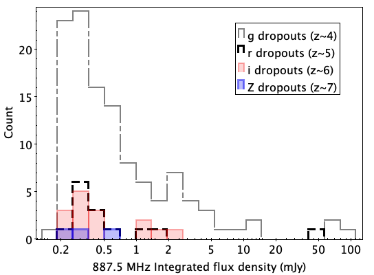
Figure 6: 887.5 MHz Total radio flux density distribution of our final sample of 148 HzRS candidates and a known radio-quasar (selected as a Z-dropout).

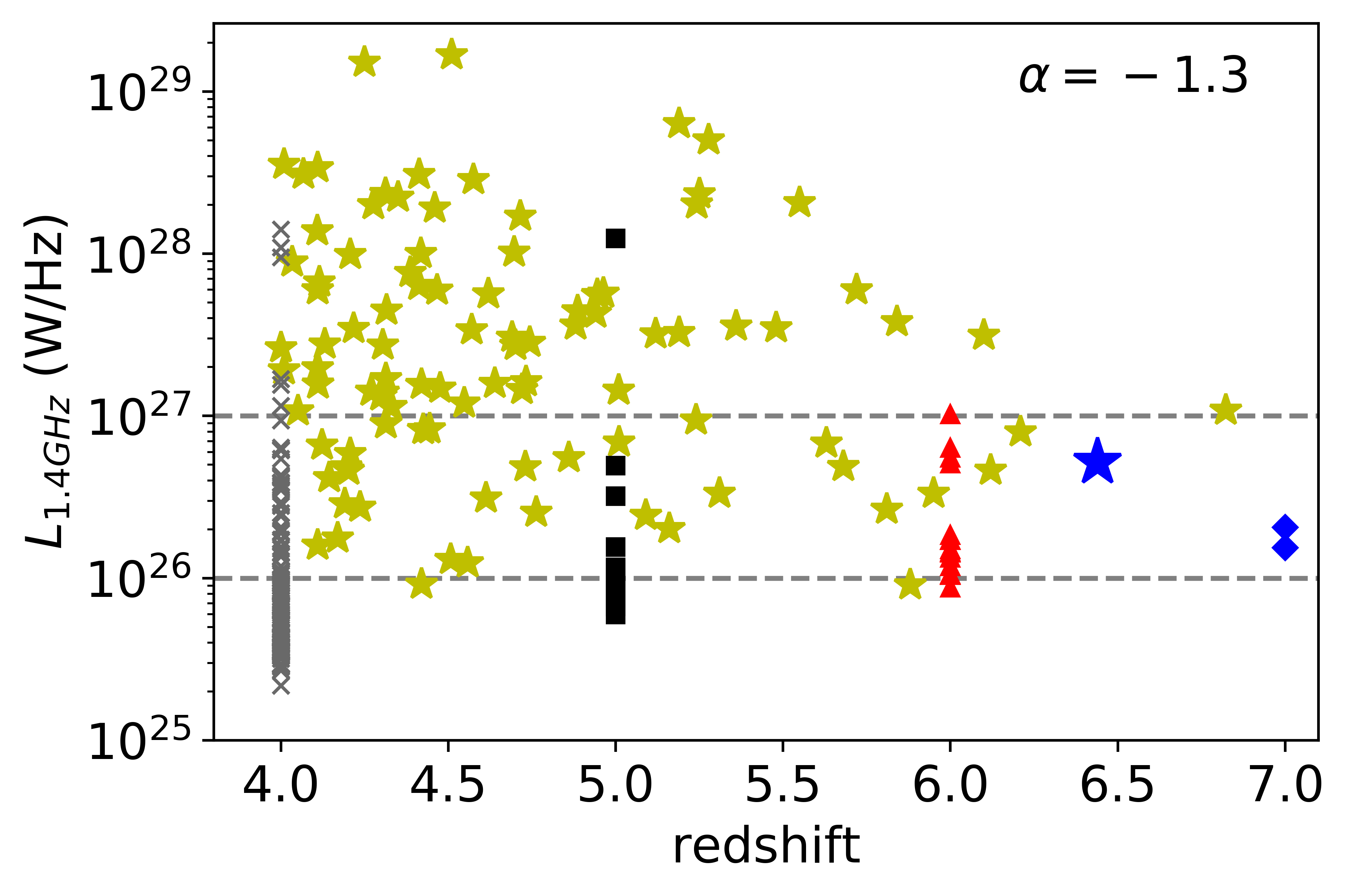
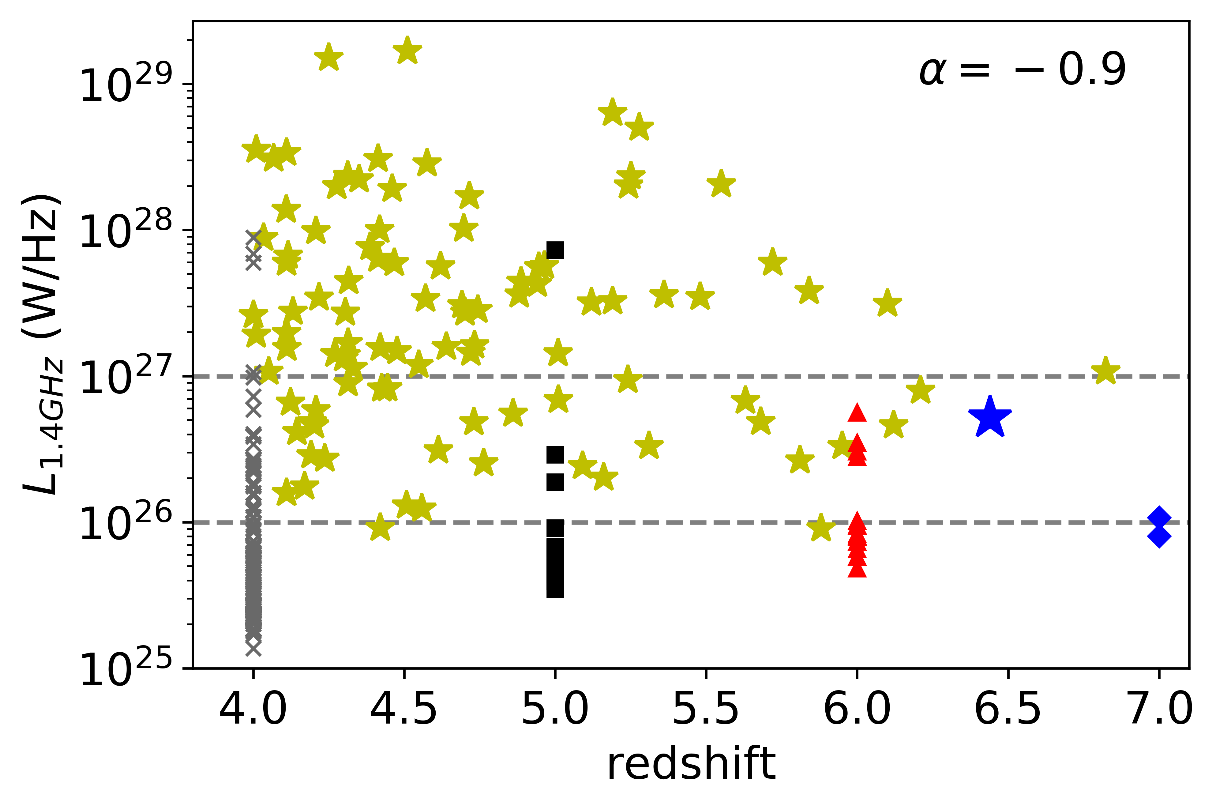
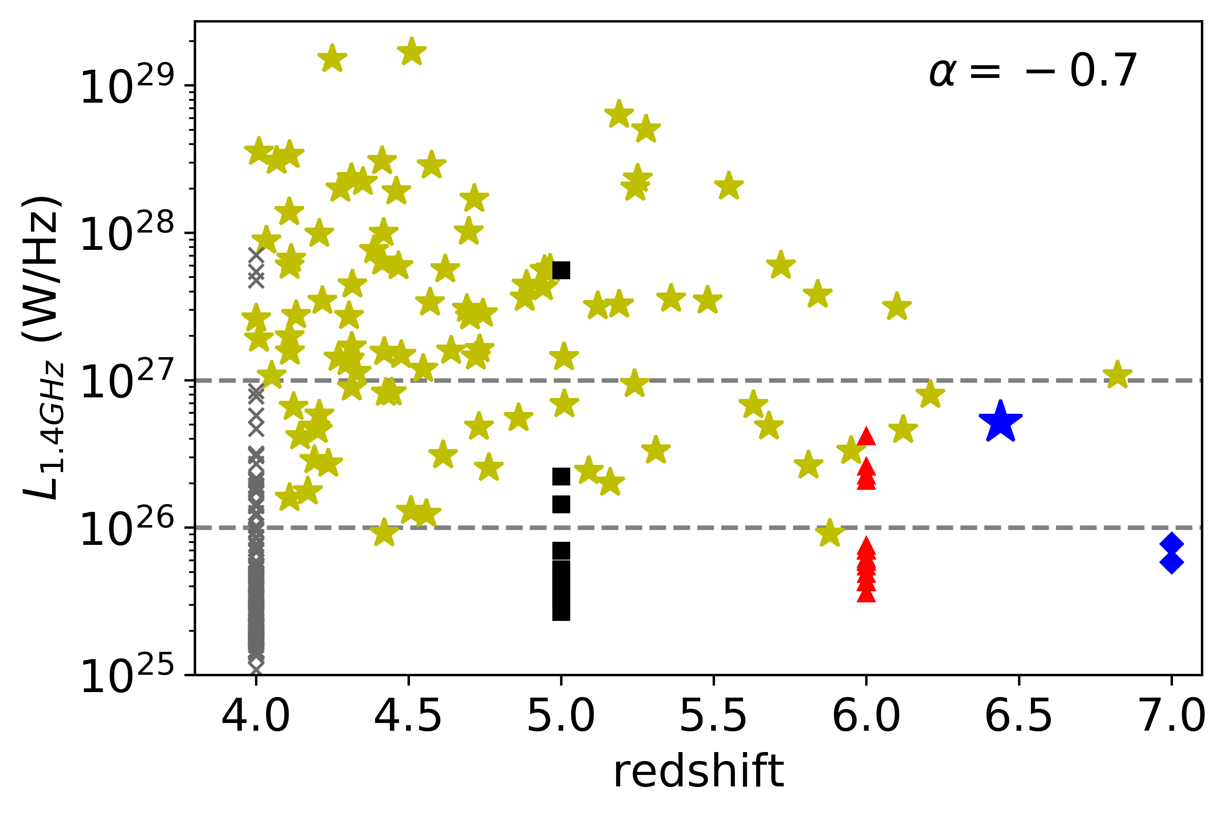
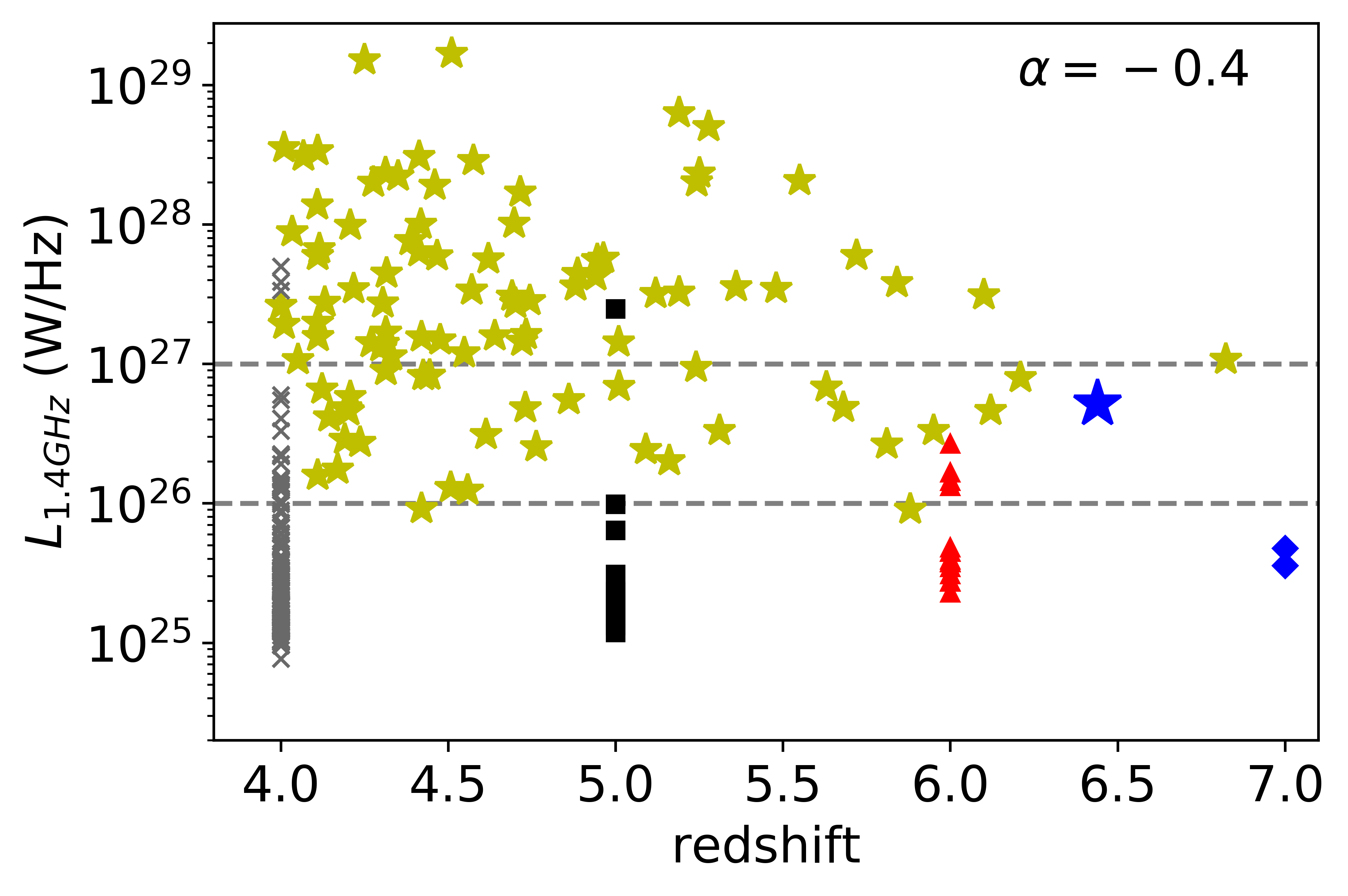
Figure 7: The 1.4 GHz radio luminosity distribution of our sample estimated for a set of spectral indices and known radio-AGNs (Appendix A, yellow stars) as a function of redshift. Irrespective of spectral index, our sample is 1-2 orders of magnitude less luminous than known AGNs at the similar redshift.

The observed 887.5 MHz flux density distribution of our final sample is shown in Figure 6. Our sample is selected from the G23 ASKAP radio catalogue and no additional radio properties are used in the selection. The distribution of flux densities of such a flux-limited sample is expected to peak at low flux densities, and this is seen in our HzRS sample, which peaks at 0.2–0.4 mJy.

Although the $z\sim 5$ and $z\sim 6$ sample are smaller, they also peak at low flux densities and follow a distribution similar to that of $z\sim 4$. We confirmed the statistical significance of this similarity by performing a Kolmogorov-Smirnov (KS) test, comparing the $z\sim 5$ and $z\sim 6$ samples with the $z\sim 4$ sample. Using the KS test, the probability that the $z\sim 5$, $z\sim 6$, and $z\sim 7$ flux density distributions are drawn from the same population as the $z\sim 4$ sample is 0.44, 0.31, and 0.65. Thus, the test suggests that the $z\sim 4$, 5, 6, and 7 sources are most likely to represent a similar type of radio source population.

We calculate the rest-frame 1.4 GHz luminosity of our sources from the total flux density observed at 887.5 MHz, using Equation 2, by assuming a power-law ($S_{\nu}\propto\nu^{\alpha}$) radio spectral energy distribution (SED) and adopting a set of radio spectral indices $\alpha=\{-1.3,-0.9,-0.7,-0.4,0.2\}$, as indicative of our complete HzRS sample. We assumed redshift, $z=$ 4, 5, 6, and 7 for g, r, i, and Z dropouts respectively in the Equation 2. The luminosity distance (D_L) is calculated using the online cosmology calculator (Wright, 2006). In other words:

$$L_{\nu_{1}} =\frac{4\pi D_{\textrm{L}}^{2}}{(1+z)^{(1+\alpha)}}\left(\frac{\nu_{1}}{\nu_{2}}\right)^{\alpha}S_{\nu_{2}}(\textrm{W/Hz}),$$ (2)

where L_$\nu$1 is the radio luminosity at rest-frame $\nu\textsubscript{1}$ derived from the observed flux density S_$\nu$2 at $\nu\textsubscript{2}$ and (1+z)^{-($1+\alpha$)} denotes the standard radio K-correction.

The resulting 1.4 GHz luminosity of our sources for a given spectral index, shown in Figure 7, as a function of redshift indicates that our sample probes less powerful HzRS compared to known radio sources (listed in the Appendix) at the same redshift. This is expected because of the greater sensitivity of the ASKAP survey. Very little is known about the properties of HzRS with $L_{1.4}<10^{26}$ W/Hz as the known HzRS are mostly brighter.

We therefore used the following diagnostics to investigate the physical origin of radio emission in our sample: (i) radio luminosity at 1.4 GHz, (ii) 1.4 GHz-to-3.4 $\mu$m flux density ratio, (iii) WISE colour, (iv) FIR detection at 250 $\mu$m, and (v) SED modelling.

4.2 1.4 GHz luminosity diagnostic

If we assume that all the radio emission is caused by star formation processes, we can calculate the star formation rate (SFR) following Bell (2003),

$$SFR(L\textsubscript{1.4}) =L\textsubscript{1.4}\times 5.52\times 10^{-22}M\textsubscript{$\odot$}/yr.$$ (3)

We show the results in Table 9.

Among extragalactic objects, Submillimeter galaxiess have the highest reported SFR: $\sim 6000~{}$M_$\odot$/yr (Barger et al., 2014). By comparison, most Lyman dropouts do not have as high SFR as SMGs, with a maximum of $\sim 300~{}$M_$\odot$/yr (Barger et al., 2014). Furthermore, Barger et al. (2014, Figure 23) demonstrated a turn-down in the observed SFR distribution function beyond 2000 M_$\odot$/yr. In Table 9, we present the SFRs estimated for each dropout at the following two flux densities at a given spectral index: (i) the minimum of 887.5 MHz flux density distribution for each dropout (ii) flux density which marks the exceeding of SFR beyond the highest known limit (6000 M_$\odot$/yr); Barger et al. (2014). In some cases, the minimum of 887.5 MHz flux density distribution itself results in an unphysical SFR. Thus, most of the SFR shown in Table 9 exceed by far the highest-known SFR of a galaxy (Barger et al., 2014), and we conclude that most of the radio emission from these galaxies is unlikely to be primarily generated by star formation, implying the presence of a radio-AGN as well.

This finding is also consistent with the simulation (Bonaldi et al., 2019; Wilman et al., 2008) of the redshift evolution of radio sources, which predicts that star forming galaxies (SFGs) are a negligible fraction of the observed radio sources beyond redshift $z>2$ at the flux limit of 0.1 mJy. We acknowledge that radio-SFR of the faintest end ($S_{887}\leq 0.2$ mJy; 5 sources) of our $z\sim 4$ sample lie in the range $\sim$4000-8000 M_$\odot$/yr, which is very high but in priciple possible given that estimated space density of SMGs with SFRs above 2000 M_$\odot$/yr is $1.4\times 10^{-5}$ M_$\odot$/yr/Mpc³ (Fu et al., 2013). Therefore, it is likely that faintest end of $z\sim 4$ sample have a Starburst (SB) component or be pure SBs.

Table 9: SFR estimated for different flux densities at $z\sim 4$, 5, 6 and 7, assuming all radio emission is powered by star formation. SFR is calculated using Equations 2 at spectral index, $\alpha=-0.8$, -0.7, -0.6 given that mean spectral index of SFGs is $\sim 0.75$

Redshift	DL	S887.5	S1.4	L1.4	SFR1.4
$z$	(103Mpc)	(mJy)	(mJy)	(W Hz-1)	(103M$\odot$/yr)
$\alpha=-0.8$
4	36.6	0.15	0.10	1.211$\times 10^{25}$	6.67
5	47.6	0.2	0.14	2.63$\times 10^{25}$	14.55
6	58.98	0.2	0.14	3.92$\times 10^{25}$	21.62
7	70.54	0.2	0.14	5.45$\times 10^{25}$	30.11
$\alpha=-0.7$
4	36.6	0.15	0.11	1.07$\times 10^{25}$	5.95
		0.2	0.15	1.44$\times 10^{25}$	7.93
5	47.6	0.2	0.15	2.31$\times 10^{25}$	12.73
6	58.98	0.2	0.15	3.37$\times 10^{25}$	18.63
7	70.54	0.2	0.15	4.64$\times 10^{25}$	25.53
$\alpha=-0.6$
4	36.6	0.15	0.11	6.9$\times 10^{24}$	3.84
		0.24	0.18	1.11$\times 10^{25}$	6.15
5	47.6	0.2	0.15	1.41$\times 10^{25}$	7.78
6	58.98	0.2	0.15	1.97$\times 10^{25}$	10.87
7	70.54	0.2	0.15	2.6$\times 10^{25}$	14.36

4.3 Radio-to-3.4 $\mu$m flux density ratio

Norris et al. (2011b, Figure 4) presented a new measure for radio-loudness of a source, 1.4 GHz-to-3.6 $\mu$m flux density ratios. They compared the 1.4 GHz-to-3.6 $\mu$m flux density ratios for different galaxy populations namely, HzRGs, SMGs, SBs, RL & RQ quasars and Ultra Luminous Infrared Galaxys, as a function of redshift. They showed that galaxies powered primarily by star forming activity have a lower ratio in contrast to radio-AGNs at all redshifts. We use 3.4 $\mu$m photometry from CATWISE2020 catalogue (Marocco et al., 2021) since there is no substantial difference between 3.4 & 3.6 $\mu$m passbands, and 3.4 $\mu$m magnitude (W1) is converted to flux density (Cutri et al., 2012) using,

$$S\textsubscript{3.4\,$\mu$m}=306.682\times 10^{-W1/2.5}~{}\textrm{Jy.}$$ (4)

.

We compare Norris et al. (2011b) model with the 1.4 GHz-to-3.4 $\mu$m flux density ratio of our sample at redshifts, $z\sim 4$, 5, and 6 in Figure 8. The measured flux density at 887.5 MHz was used to estimate the 1.4 GHz flux density, assuming spectral indices, $\alpha$ of -1.3, -0.7, and 0.2 as indicative of our entire HzRS sample. According to that model, radio-AGNs have a radio-to-3.6 $\mu$m flux density ratio above 100 at all redshifts. However, Maini et al. (2016) showed that the ratio for Type 1 & 2 AGN/QSO and high power radio galaxies start to decrease (between 10 and 100) beyond $z\sim 4$ and $z\sim 5$ . We contend that reason for this difference is that the Norris et al. (2011b) model refers to powerful radio-AGNs only, at all redshifts. About $55\%$ of our sample have a 1.4 GHz-to-3.4 $\mu$m flux density ratio between 1 and 10 and $\sim 41\%$ between 10 and 100. Only 5 sources in our sample have a radio-to-3.4 $\mu$m ratio greater than 100.

It therefore seems that high-$z$ radio-AGNs can extend to even lower values ($<10$) of radio/IR ratios than previously thought. The following are some possible explanations for their low ratio: (i) radio-AGN is accompanied by SB activity, and the optical emission being redshifted to W1 band causing an increase in the 3.4 $\mu$m flux density (ii) the inherently low radio powers of high-$z$ radio-AGNs, as predicted by simulation in Saxena et al. (2017) (iii) optical emission from un-obscured quasars at $z\geq 4$ being redshifted to W1 band. We discuss this further in Section 4.4.2.

Figure 8: 887.5 MHz flux density vs. 3.4 $\mu$m flux density for $z\gtrsim 4$ sample, colour coded according to their 1.4 GHz-to-3.4 $\mu$m flux density ratio. 1.4 GHz flux density is estimated from observed flux density at 887.5 MHz assuming spectral indices, $\alpha=-1.3$, – 0.7, 0.2.

4.4 FIR detection

Dust heated by stars or AGN generally re-radiates the absorbed energy at FIR wavelengths. Each galaxy will have a distribution of dust temperatures which is determined by the size and distribution of dust with respect to the heating source ( Star Formation (SF) or AGN). Cool ($T\sim 20\,K$) dust arises from the diffuse interstellar medium (ISM), warm ($T\sim 40\,K$) dust from SF regions, and even warmer $T\sim 60-100\,K$ dust results from AGN activity.

We queried the Herschel database to check whether any of our sources have been detected at FIR wavelengths. We searched the SPIRE point source catalogues at 250 $\mu$m, 350 $\mu$m, and 500 $\mu$m (Schulz et al., 2017) separately in a 5 arcsec cone around the WISE position of each of our HzRS sample, which yielded a false-id rate of $\sim 16\%$. Several of our sources have a SPIRE counterpart, but none was found in the PACS point source catalogues. A total of 14 and 3 sources from our $z\sim 4$ and $z\sim 6$ sample respectively were found to have a SPIRE counterpart, representing only 10% of our entire HzRS sample.

We present the results in Table 10. The SPIRE 250 $\mu$m band probes a rest wavelength $\sim$45 - 63 $\mu$m at $z=3-4.3$ ($g$ dropouts) and $\sim$34 - 38 $\mu$m at $z=5.6-6.2$ ($i$ dropouts). At wavelength $<50$ $\mu$m in the rest-frame, an AGN heated dust torus may contribute significantly to the FIR emission. Therefore the SPIRE detection of our radio sources suggests that the observed 250 $\mu$m emission may arise from either (i) a dust torus heated by an AGN or (ii) SB activity or (iii) a combination of both SF and AGN.

Table 10: Our HzRS with a FIR detection in either of Herschel-SPIRE 250 $\mu$m, 350 $\mu$m $\&$ 500 $\mu$m bands, selected from a 5 arcsec search around their WISE position at which false-ID rate is $\sim 16\%$. The probability of a source’s measured SPIRE flux being contaminated by a nearby neighbour is about 1/14.

Source ID	S250	S350	S500
	(mJy)	(mJy)	(mJy)
$z\sim 4$ candidates
J224308-313622	59.3
J223533-343305	67.4	40.7	–
J231210-332436	49.9	32.3	–
J224203-333606	59.5	68.5	–
J231826-323746	39.9	–	–
J223729-325838	34.8	–	–
J224017-325128	66.2	–	–
J224552-312733	51.2	–	–
J225343-313305	65.4	–	–
J231648-303629	65.6	–	–
J232019-294205	93.6	77.2	–
J232135-320117	44.5	–
J225915-314116	–	78.1	62.9
J224955-294536	–	–	49
$z\sim 6$ candidates
J224652-340238	92.9	62.4	47.9
J231245-291817	98.5	86.8	48.9
J223719-333857	65.6	52.5	–

4.4.1 Radio-FIR relation

In this section, we explore the 250 $\mu$m-to-1.4 GHz luminosity ratio of our sources, as defined by Equation 5, which is a tracer of star formation activity. Here we are only interested in order-of-magnitude estimates and hence we neglect evolution. Another paper in which we model evolutionary effects is in preparation. $q\textsubscript{250}$ is defined as:

$$q_{250}=\log_{10}\left(\frac{L_{250}}{L_{1.4}}\right)~{},$$ (5)

where $L\textsubscript{250}$ and $L\textsubscript{1.4}$ are the rest-frame luminosities at 250 $\mu$n and 1.4 GHz respectively.

To estimate rest-frame $L\textsubscript{250}$, we must first estimate the K-correction (k_corr) defined as

$$k_{corr}=\frac{S_{rest}}{S_{obs}}~{},$$ (6)

where $S_{\rm obs}$ and $S_{\rm rest}$ are the observed and the rest-frame flux densities respectively.

Assuming a greybody thermal emission, the spectral flux density at a given frequency and temperature, $S_{\nu}(T)$, would be a modified Planck’s radiation law $B(\nu,T)$,

$$S_{\nu}(T) \propto\nu^{\beta}B(\nu,T)~{},$$ (7)

where

$$B(\nu,T) =\frac{2h}{c^{2}}\frac{\nu^{3}}{e^{\frac{h\nu}{k_{B}T}}-1}$$ (8)

and $\beta$ represents the dust emissivity index, for which we assume a value of 1.5 (Kirkpatrick et al., 2015).

We calculate the K-correction using Equations 6, 7 and 8, assuming 2 dust temperatures, 45  K, $\&$ 80 K, corresponding to warm and warmer dust components based on Kirkpatrick et al. (2015) study, and present the results in Table 11.

Table 11: K-correction estimated for the observed frame at 250 $\mu$m, assuming the dust emission either dominated by a warmer dust ($T_{w}\sim$ 80 K) or a warm dust ($T_{w}\sim$ 45 K).

redshift	$\nu$obs	$\lambda$rest	$\nu$rest	kcorr
($z$)	(Hz)	($\mu$m)	(Hz)
$T_{dust}\sim 45\,K$
4	$1.2\times 10^{12}$	50	$5.9\times 10^{12}$	6.22
5		42	$7.2\times 10^{12}$	3.8
6		36	$8.4\times 10^{12}$	2.11
$T_{dust}\sim 80\,K$
4	$1.2\times 10^{12}$	50	$5.9\times 10^{12}$	40.77
5		42	$7.2\times 10^{12}$	44.93
6		36	$8.4\times 10^{12}$	43.46

We then calculate the luminosity $L_{250}$,

$$L_{250}=\frac{4\pi S_{250}K_{cor}D_{\textrm{L}}^{2}}{1+z}~{},$$ (9)

where $S_{250}$ is the observed flux densities of our sources in the SPIRE database and D_L is the luminosity distance.

The resulting $q\textsubscript{250}$ estimated for two extremes of assumed radio spectral indices (see Section 4.1) is shown in Figure 9. All sources with a reliable detection as indicated by SNR>5 and 3>SNR>5 have q₂₅₀ exceeding the threshold of 1.3 (Jarvis et al., 2010; Virdee et al., 2013) indicating luminous SFG. The high values of $q\textsubscript{250}$, irrespective of radio spectral index, suggest the presence of an active SB component in SPIRE detected sources but on the other hand our K-correction is very uncertain because of our lack of knowledge of the FIR SED, and so we do not consider this a definitive indicator of SF. Furthermore, SPIRE detected sources have $S_{887.5}>0.2$ mJy implying the presence of a radio-AGN component according to Table 9. Therefore, we attempt to estimate SFR (see Section 4.4.2), from the observed 250 $\mu$m emission to verify whether the resulting SFR is sufficient enough to generate the observed radio luminosity. We also note that q₂₅₀ criterion is based on the study of powerful radio-AGNs in the literature, whereas this study probe low power radio-AGNs, suggesting q${}_{250}>1.3$ may not be applicable in this case.

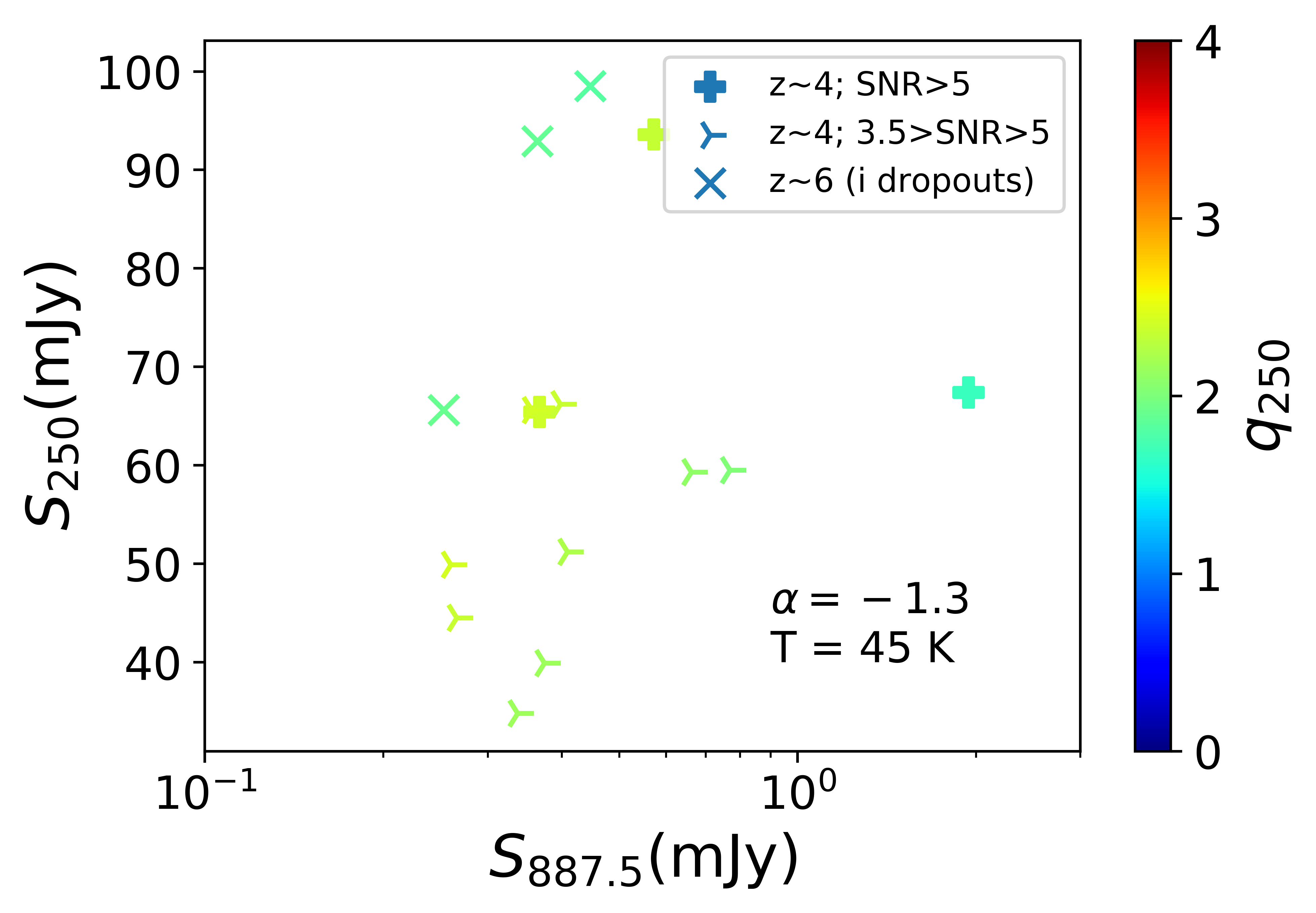
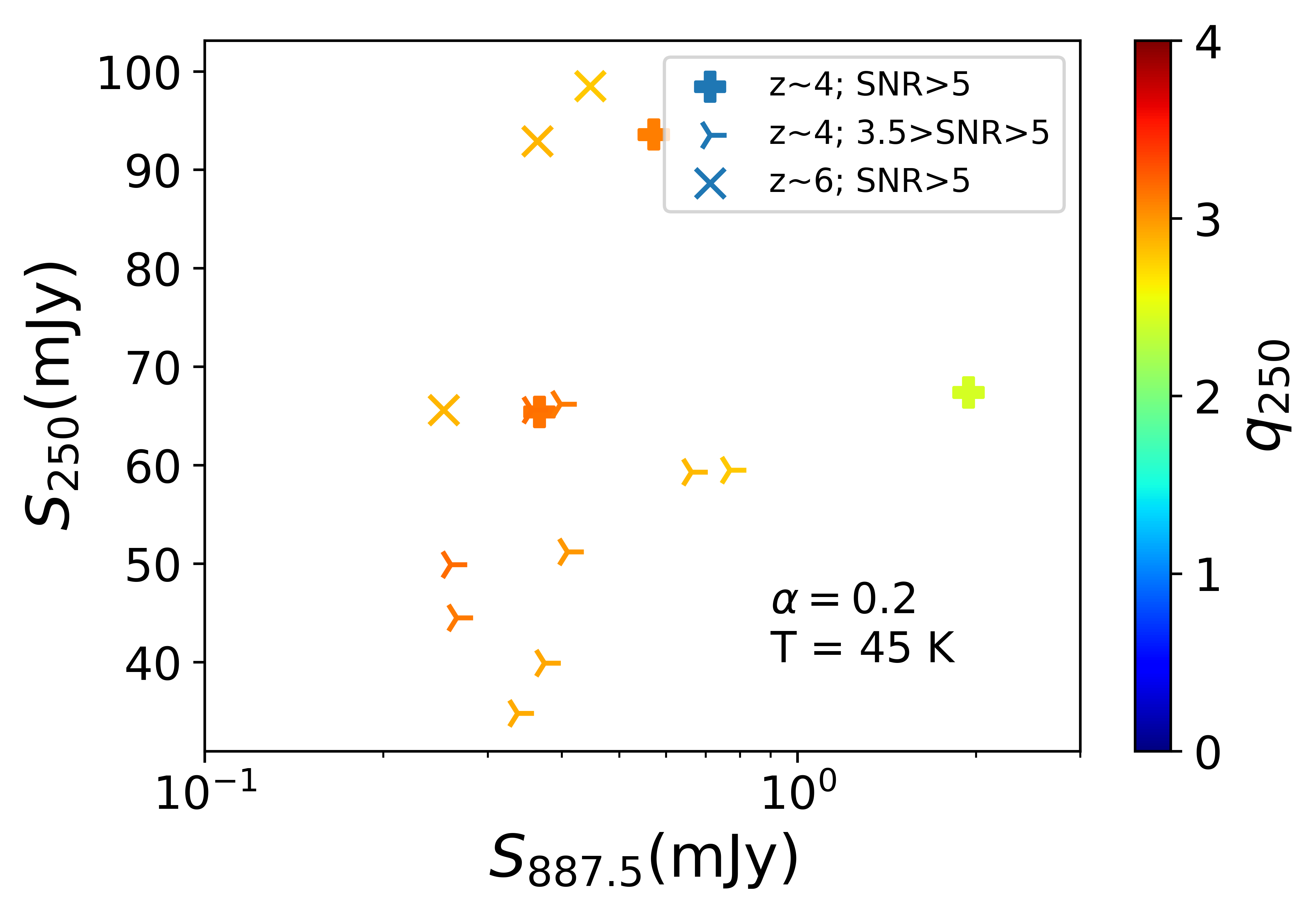
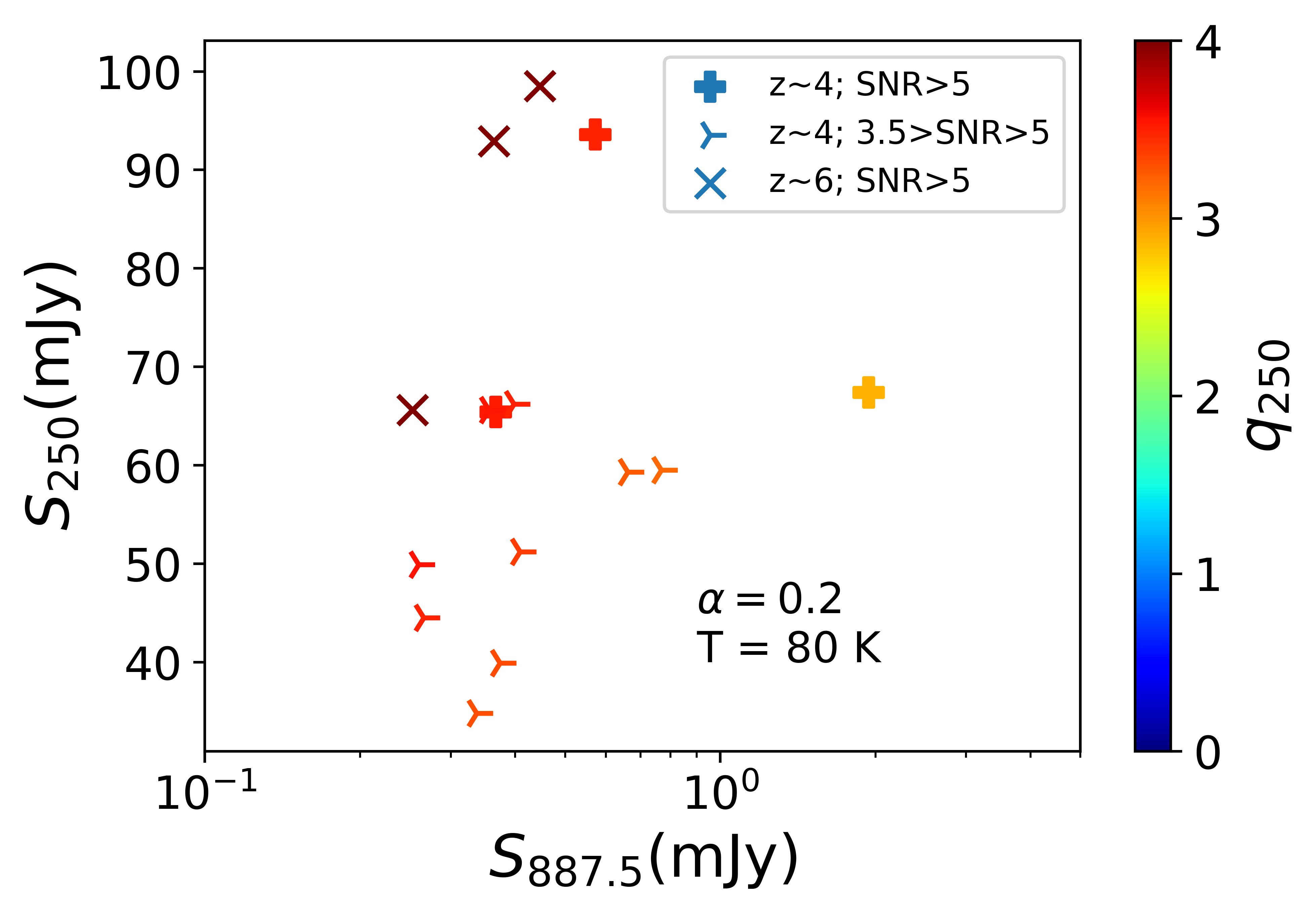
Figure 9: 887.5 MHz flux density vs. 250 $\mu$m flux density for $z\gtrsim 4$ sample, colour coded according to their q₂₅₀ measurements.

4.4.2 SFR from S₂₅₀

We estimate the SFR from S₂₅₀ via the rest-frame 24 $\mu$m luminosity, $L_{24\,\mu m}$ (in erg/s), using the following equations from Brown et al. (2017),

$$\log L_{24_{\mu m}} =40.93+1.3(\log L_{H\alpha}-40)$$ (10)

$$SFR =L_{H\alpha}\times 5.5\times 10^{-42}~{}\rm{M_{\odot}/yr}~{}.$$ (11)

For the calculation of $\text{L}_{24\,\mu m}$, we consider 4 different spectral energy distribution (SED) models corresponding to: (i) an ultra luminous infrared galaxy (Arp 220), (ii) a starburst (M 82), (iii) Mrk 231 (luminous infrared AGN), and (iv) a composite system (IRAS F00183–7111), in which the optical/IR SED is dominated by the starburst surrounding the AGN, with the AGN emerging only at radio wavelengths (Norris et al., 2012a). In each case, we interpolate the SED using flux density measurements obtained via NASA/IPAC Extragalactic Database (NED).

We perform the following calculations to estimate $\text{L}_{24\,\mu m}$ of our sources:

1. We calculate the luminosity of our sources corresponding to their emitted wavelengths from their observed flux density at 250 $\mu$m using the equation,

   $L_{\lambda}=\frac{4\pi D_{\textrm{L}}^{2}S_{250}}{1+z}$,
   where $\lambda$ represents the respective emitted (or rest-frame) wavelength at $z\sim 4,5,6$ as shown in column 3 of Table 11.

2. For each model source (Arp 220, M 82, Mrk 231, IRAS F00183–7111) we assume that the ratio $L_{24\mu m}/L_{\lambda}$ for our sources is the same as that of the model source as measured from their SED:

   $\left(\frac{L_{24\mu m}}{L_{\lambda}}\right)_{oursource}$ = $\left(\frac{S_{24\mu m}}{S_{\lambda}}\right)_{model}$.

Figure 10: SFR estimated from S₂₅₀ by assuming various SED models.

We present the results of this calculation in Figure 10. The resulting SFRs for $z\sim 4$ & $z\sim 6$ samples lie in the range $\sim 400-3500$  M_$\odot$/yr & $\sim 2000-8200$  M_$\odot$/yr respectively, which is high but not unphysical, and similar to the SFRs reported for SBs and SMGs at similar redshifts (Barger et al., 2014). These SFRs would generate a radio power in the order of $\sim 10^{24}-10^{25}$ W Hz^-1, which is typically a small fraction ($\leq 10\%$) of the observed radio luminosities.

We conclude that these galaxies detected by Herschel-SPIRE are likely to be composite galaxies containing both a radio-AGN and a starburst. We further note that the radio-to-3.4 $\mu$m flux density ratio of SPIRE detected sources is $<100$. 7 out of 15 250 $\mu$m detected sources found to have $W1-W2>0.8$ WISE colour, suggesting an AGN component. At $z\gtrsim 4$, W1 WISE band observations probe the optical rest-frame including H$\alpha$ emission, an indicator of SF activity or quasar light or both. This suggests that a fraction of high-$z$ radio-AGNs ($\log L\textsubscript{1.4}=25$) at $z\gtrsim 4$ may have a SB host, contrary to low-z radio-AGNs which are usually hosted by quiescent galaxies. Similarly, Rees et al. (2016) found that $z>1.5$ radio-AGNs tend to be hosted by SFGs. Our study suggests that this may be true at even higher redshifts.

4.5 WISE colours

Mid-IR colour selection criteria are an efficient tool to identify a hot accretion disk, which is an indicator of AGN in galaxies. The dust reprocesses the emission from the accretion disk into the IR, which dominates the AGN SED at wavelengths from $\sim 1$ $\mu$m to a few tens of microns, the wavelength regime covered by the WISE survey.

Stern et al. (2012) demonstrated that a simple WISE colour cut, $W1-W2>0.8$, selects AGN with a reliability of 95% and with a completeness of 78%. However, this colour cut works efficiently for low-z sources ($z\sim 1$) only, given that is defined using observed fluxes not rest-frame ones. Stern et al. (2012) therefore discussed a number of possible scenarios to interpret W1-W2 colour at higher redshifts.

Following are the possibilities, taken from Stern et al. (2012), applicable to our $z\gtrsim 4$ sample,

1. At $z\gtrsim 3.5$, W1/W2 bands probe optical & near-IR rest-frame emission causing the $\sim 1$ $\mu$m minimum seen in some starburst galaxies shifting to W2 band and H$\alpha$ emission shifting to W1. This results in a blue W1-W2 (<0.8) colour

2. A highly obscured AGN will have $W1-W2>0.8$ at all redshifts.

3. For a composite system (AGN $+$ SB), dilution by host-galaxy light can limit the identification of low luminosity AGNs.

We looked at the W1-W2 colour of our sources, utilizing CATWISE magnitudes. We considered only those sources without any flags and with SNR$\geq$5 in the W1 and W2 bands. This identifies 106 sources, of which only 28 sources satisfy the $W1-W2>0.8$ AGN criterion. We further found that all but 2 of the sources satisfying the $W1-W2>0.8$ AGN criterion have S₈₈₇$\gtrsim$0.2-2.5 mJy and 1.4 GHz-to-3.4 $\mu$m flux density ratio between 1 and 100. This supports our argument that (i) low power radio sources in our sample are powered by a radio-AGN (ii) the radio-to-IR flux density ratio of low power radio-AGNs can extend to lower values (<100). On the other hand, the sources with $W1-W2<0.8$ could be either unobscured quasars, as they have a blue $W1-W2$ colour at high-$z$ as demonstrated in Ross & Cross (2020) or the composite galaxies where the SB component results in a blue $W1-W2$ colour. In addition to this, we verified the WISE magnitudes of a known starbust at $z=4.1$ (Ciesla et al., 2020) and found that its $W1-W2=0.63$ matches our $z\gtrsim 4$ sample with S_1.4$<$1 mJy.

4.6 SED modelling

It is beyond the scope of this paper to perform full SED modelling of these galaxies, but here we make an illustrative comparison of these galaxies with two representative low-redshift galaxies. To do so, we shift two local radio sources to $z\gtrsim 4$ for comparison: (i) Cygnus A, a radio galaxy at $z=0.05607$, and (ii) IRAS F00183–7111, an ultraluminous infrared galaxy (ULIRG) at $z=0.327$ showing composite emission from a radio loud-AGN and a SB. Each of these sources is distinct: their radio emission either comes from an AGN or a combination of SF and AGN. Their broadband observed photometry is obtained from NED. We added more radio data from Norris et al. (2012b, Table 1) to the IRAS F00183–7111 template since the radio coverage is poor and this wavelength regime is critical for this analysis.

We do not consider galaxies exclusively powered by star formation activity, like M 82 and Arp 220, as they produce radio flux densities three or four orders of magnitude below the current detection limit when shifted to $z\gtrsim 4$, indicating that none of our sources represent typical SFGs.

We create the SED at $z\gtrsim 4$ by shifting the observed SED in the frequency space by a factor of (1+$z$)^-1, and in flux density space by a factor of (D_obs/D_z)²$\times{\it(1+z_{\rm{\it shift}}}/{\it 1+z_{\rm{\it obs}}})$. D_obs and D_z are the luminosity distance to the observed redshift and shifted redshift ($z_{\rm{\it shift}}\sim 4$, 5, 6 or 7) respectively, estimated using an online cosmology calculator (Wright, 2006).

Figure 11 shows the resulting shifted SEDs. The extracted 1.4 GHz flux density from the shifted SEDs, shown in Table 12, demonstrates that (i) active galaxies powered by a radio-AGN, such as Cygnus A, can represent the brighter sources in our sample and (ii) a composite system like IRAS F00183-7111 consisting of a radio-AGN and a significant SB component, can represent fainter sources in our sample. Thus, our SED modelling shows that a radio-AGN and a composite system can reproduce the galaxies in our sample implying that properties of our HzRS are not that extraordinary compared to typical local galaxies. At the same time, we note that IRAS F00183-7111 does not reproduce our sample’s observed SPIRE flux densities, as its SFR ($\sim 220$ $M_{\odot}$/yr; Mao et al. (2014)) is not sufficient.

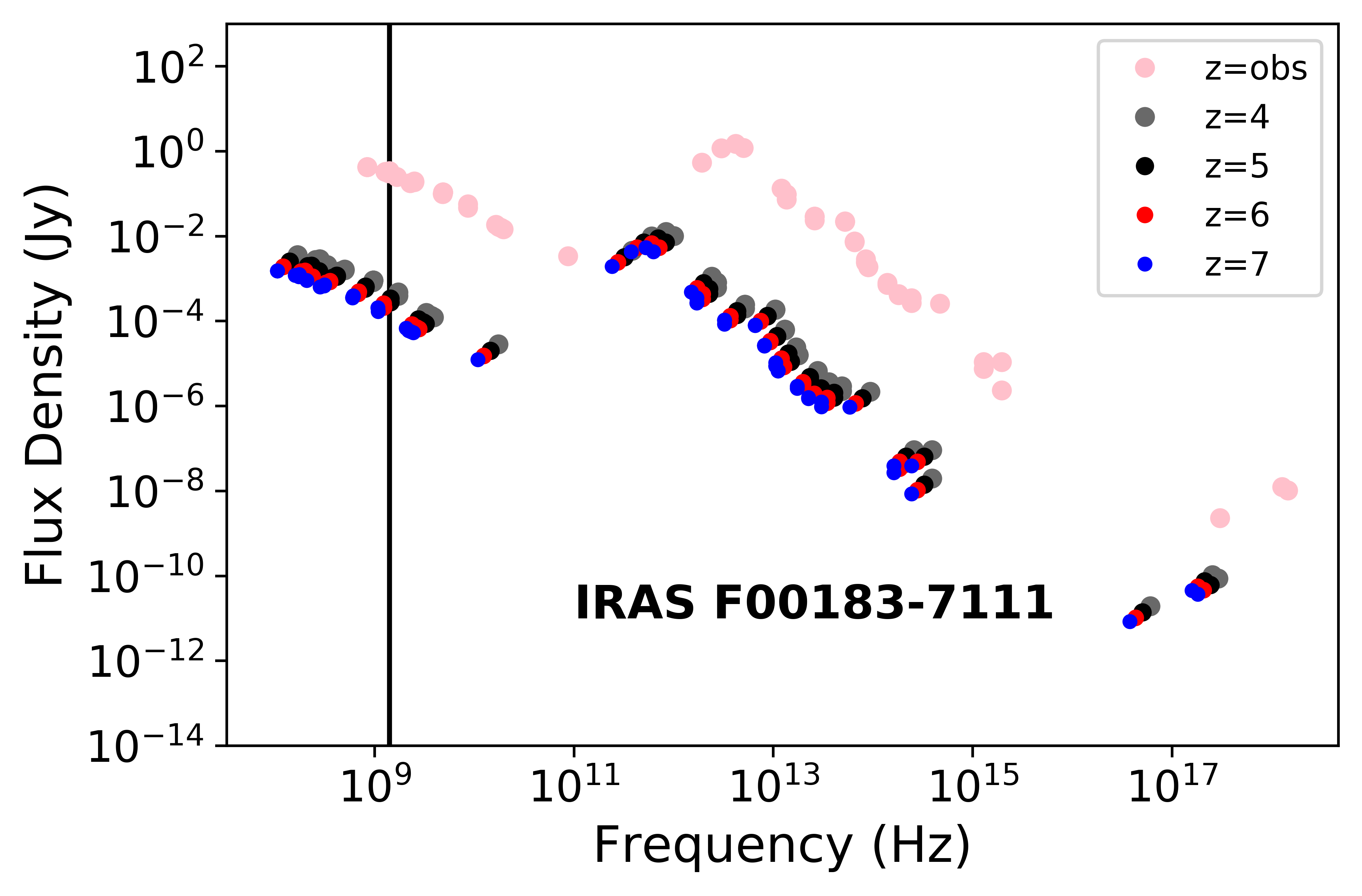
Figure 11: Template SEDs shifted to redshifts, $z=4,5,6,7$ in grey, black, red and blue colours respectively. SED templates are built by simply connecting the datapoints and performed 1D interpolation using python-scipy (interp1d) package to obtain 1.4 GHz flux density information from the shifted SEDs. 1.4 GHz is marked in black solid line. Pink points represent the observed SED, obtained from NED.

Table 12: 1.4 GHz flux density extracted from the template SEDs shifted to $z=4,5,6$ by performing 1d interpolation using interp1d function in python-scipy package.

Source	S1.4 (mJy)
	$z\sim 4$	$z\sim 5$	$z\sim 6$	$z\sim 7$
Cygnus A	60	29	20	14
IRAS F00183	0.6	0.3	0.2	0.1

5 Conclusions

We have used the Lyman dropout technique to identify a sample of 149 radio sources at $z\gtrsim 4-7$, of which one is a known radio-quasar (VIK J2318-3113; selected as a Z-dropout) at $z=6.44$, and 148 are newly-identified. Our study reveals a new population of high-redshift ($z\sim$ 4–7) radio-AGNs, $\sim 1-2$ orders of magnitudes fainter than currently known radio-AGNs at similar redshifts, but with 1.4 GHz luminosities typical of lower-redshift radio-loud AGN.

Comparison with spectroscopic redshifts in the COSMOS field indicate that our $z\sim 4$ sample is about 88% reliable, the $z\sim 5$ sample is about 81% reliable, and the $z\sim 6$ sample is at least about 62% reliable. We do not have a reliability estimate for the $z\sim 7$ sample.

We have explored radio and IR observations to understand the origin of the radio emission of our HzRS sample. Our conclusions are as follows.

1. The radio (1.4 GHz) estimated SFR of our sample (Table 9) gives unphysical values, indicating that radio emission in our sources is not solely powered by star formation.

2. The faint ($\log L\textsubscript{1.4}=25$) and bright ($\log L\textsubscript{1.4}\geq 26$) end of our sample spans the low and high power radio galaxy luminosity classes respectively, suggesting the presence of a radio-AGN component in our sample. This study presents a new population of less powerful radio-AGNs candidates at $z\sim 4$, 5 and 6 that have been missed by previous surveys.

3. $\sim 10\%$ of our HzRS sample are detected in the Herschel-SPIRE bands which probe SB heated dust emission and AGN heated dust torus emission at $z>2$. This suggests that SPIRE detected sources are likely to represent composite systems.

4. We demonstrate that some high-$z$ radio-AGNs tend to have hosts that are SB galaxies, in contrast to low-$z$ radio-AGNs, which are usually hosted by quiescent elliptical galaxies.

5. Using the $W1-W2>0.8$ AGN indicator, we identified 28 radio-AGNs, 26 of which are found to be on the faint end of the observed 887.5 MHz flux density distribution. We further demonstrate that the 1.4 GHz-to-3.4 $\mu$m flux density ratio of these weak radio-AGNs extends to lower values (1-100) than previously thought.

6. SED modelling confirms that a composite system (radio-AGN $+$ SB) and a radio galaxy at $z\gtrsim 4$ can produce the radio flux densities similar to ones observed at the faint and bright end respectively.

6 Future work

Spectroscopic follow-up of our sample is essential (i) to confirm the redshifts of these candidate sources identified by the Lyman dropout technique (ii) to verify the reliability of magnitude cut-off introduced in $Z$-band for $i$ dropouts (iii) to establish the criteria to identify interlopers, if present. The above three goals are critical in producing reliable criteria to select HzRS in the full EMU survey and thus verifying the model (Raccanelli et al., 2012) for the redshift distribution of radio sources.

Data Availability

This study utilised the data available in the following public domains:

1. https://data.csiro.au/domain/casdaObservation

2. https://kids.strw.leidenuniv.nl/DR4/access.php

3. http://horus.roe.ac.uk/vsa/index.html

4. https://irsa.ipac.caltech.edu/

The derived final datasets are available in the article.

Appendix A Tables

Table A.1: Example for the list of published radio-AGNs at z$\geq$4. The full catalogue is available online.

Index	Name	RA	DEC	redshift	S1.4	class	Reference
		(deg)	(deg)	z	(mJy)
1	NVSS J153050+104932	232.70867	10.82558	5.720	7.5	radio galaxy	Saxena et al. (2018)
2	J085614+022359	134.0583	2.3997	5.55	86.5	radio galaxy	Drouart et al. (2020)
3	TN J0924-2201	141.08300	-22.02819	5.190	71.5	radio galaxy	De Breuck et al. (2001)
4	FIRST J163912.1+405236	249.80045	40.87686	4.880	22	radio galaxy	Jarvis et al. (2009)
5	HSC J083913.17+011308.1	8.65366	1.21892	4.72	7.17	radio galaxy	Yamashita et al. (2020)
$--$	$--$	$--$	$--$	$--$	$--$	$--$	$--$

Table A.2: A list of 33 new radio sources at $z\gtrsim 4$, obtained by cross-matching SDSS and FIRST/NVSS. In each case the SDSS spectrum has been checked for supporting evidence of the redshift, such as the Lyman break or other spectral features. The full catalogue is available online.

Index	Name	RA	DEC	redshift	S1.4	class	Reference
		(deg)	(deg)	z	(mJy)
1	SDSS J1148+5251	177.06935	52.86395	6.420	0.055	qso	Walter et al. (2004)
2	SDSS J100831.57+401910.3	152.13150	40.31947	5.670	2.52	galaxy
3	2MASX J00300536+2957082	7.52242	29.95225	5.199	17.7	qso	Waldram et al. (2007)
4	SDSS J085826.55+553234.9	134.6107	55.54291	5.076	20.6	qso
5	J142634.86+543622.8	216.64524	54.60634	4.848	4.36	qso	Wang et al. (2016)
$--$	$--$	$--$	$--$	$--$	$--$	$--$	$--$

References

- Alam et al. (2015) Alam S., et al., 2015, ApJS, 219, 12
- Baldry et al. (2018) Baldry I. K., et al., 2018, MNRAS, 474, 3875
- Banados et al. (2018) Banados E., et al., 2018, Nature, 553, 473
- Bañados et al. (2021) Bañados E., et al., 2021, The Astrophysical Journal, 909, 80
- Barger et al. (2014) Barger A., et al., 2014, The Astrophysical Journal, 784, 9
- Becker et al. (1995) Becker R. H., White R. L., Helfand D. J., 1995, ApJ, 450, 559
- Bell (2003) Bell E. F., 2003, ApJ, 586, 794
- Belladitta et al. (2020) Belladitta S., et al., 2020, Astronomy & Astrophysics, 635, L7
- Bonaldi et al. (2019) Bonaldi A., Bonato M., Galluzzi V., Harrison I., Massardi M., Kay S., De Zotti G., Brown M. L., 2019, Monthly Notices of the Royal Astronomical Society, 482, 2
- Brown et al. (2017) Brown M. J., et al., 2017, The Astrophysical Journal, 847, 136
- Brown et al. (2020) Brown A. G., Vallenari A., Prusti T., De Bruijne J., Babusiaux C., Biermann M., Collaboration G., et al., 2020, arXiv preprint arXiv:2012.01533
- Capak et al. (2007) Capak P., et al., 2007, The Astrophysical Journal Supplement Series, 172, 99
- Ciesla et al. (2020) Ciesla L., et al., 2020, Astronomy & Astrophysics, 635, A27
- Condon et al. (1998) Condon J. J., Cotton W. D., Greisen E. W., Yin Q. F., Perley R. A., Taylor G. B., Broderick J. J., 1998, AJ, 115, 1693
- Cutri et al. (2012) Cutri R., et al., 2012, Explanatory Supplement to the WISE All-Sky Data Release Products, p. 1
- De Breuck et al. (2000) De Breuck C., Van Breugel W., Röttgering H. J., Miley G., 2000, Astronomy and Astrophysics Supplement Series, 143, 303
- De Breuck et al. (2001) De Breuck C., et al., 2001, The Astronomical Journal, 121, 1241
- Driver et al. (2008) Driver S. P., et al., 2008, Proceedings of the International Astronomical Union, 4, 469
- Drouart et al. (2020) Drouart G., et al., 2020, Publications of the Astronomical Society of Australia, 37
- Flesch (2021) Flesch E. W., 2021, arXiv e-prints, p. arXiv:2105.12985
- Fu et al. (2013) Fu H., et al., 2013, Nature, 498, 338
- Griffin et al. (2010) Griffin M. J., et al., 2010, Astronomy & Astrophysics, 518, L3
- Hasinger et al. (2018) Hasinger G., et al., 2018, The Astrophysical Journal, 858, 77
- Hatziminaoglou et al. (2010) Hatziminaoglou E., et al., 2010, Astronomy & Astrophysics, 518, L33
- Ighina et al. (2021) Ighina L., Belladitta S., Caccianiga A., Broderick J., Drouart G., Moretti A., Seymour N., 2021, Astronomy & Astrophysics, 647, L11
- Jarvis et al. (2009) Jarvis M. J., Teimourian H., Simpson C., Smith D. J., Rawlings S., Bonfield D., 2009, Monthly Notices of the Royal Astronomical Society: Letters, 398, L83
- Jarvis et al. (2010) Jarvis M. J., et al., 2010, Monthly Notices of the Royal Astronomical Society, 409, 92
- Johnston et al. (2007) Johnston S., et al., 2007, Publications of the Astronomical Society of Australia, 24, 174
- Kirkpatrick et al. (2015) Kirkpatrick A., Pope A., Sajina A., Roebuck E., Yan L., Armus L., Díaz-Santos T., Stierwalt S., 2015, The Astrophysical Journal, 814, 9
- Kuijken et al. (2015) Kuijken K., et al., 2015, Monthly Notices of the Royal Astronomical Society, 454, 3500
- Kuijken et al. (2019) Kuijken K., et al., 2019, Astronomy & Astrophysics, 625, A2
- Laigle et al. (2016) Laigle C., et al., 2016, The Astrophysical Journal Supplement Series, 224, 24
- Maini et al. (2016) Maini A., Prandoni I., Norris R. P., Spitler L. R., Mignano A., Lacy M., Morganti R., 2016, Astronomy & Astrophysics, 596, A80
- Mao et al. (2014) Mao M. Y., Norris R. P., Emonts B., Sharp R., Feain I., Chow K., Lenc E., Stevens J., 2014, Monthly Notices of the Royal Astronomical Society: Letters, 440, L31
- Marocco et al. (2021) Marocco F., et al., 2021, The Astrophysical Journal Supplement Series, 253, 8
- Marton et al. (2017) Marton G., et al., 2017, arXiv preprint arXiv:1705.05693
- Miley & De Breuck (2008) Miley G., De Breuck C., 2008, The Astronomy and Astrophysics Review, 15, 67
- Mortlock et al. (2011) Mortlock D. J., et al., 2011, Nature, 474, 616
- Norris et al. (2011a) Norris R. P., et al., 2011a, Publications of the Astronomical Society of Australia, 28, 215
- Norris et al. (2011b) Norris R. P., et al., 2011b, The Astrophysical Journal, 736, 55
- Norris et al. (2012b) Norris R. P., Lenc E., Roy A. L., Spoon H., 2012b, Monthly Notices of the Royal Astronomical Society, 422, 1453
- Norris et al. (2012a) Norris R. P., Lenc E., Roy A. L., Spoon H., 2012a, MNRAS, 422, 1453
- Norris et al. (2021) Norris R. P., et al., 2021, arXiv e-prints, p. arXiv:2108.00569
- Ono et al. (2018) Ono Y., et al., 2018, Publications of the Astronomical Society of Japan, 70, S10
- Poglitsch et al. (2010) Poglitsch A., et al., 2010, Astronomy & astrophysics, 518, L2
- Raccanelli et al. (2012) Raccanelli A., et al., 2012, Monthly Notices of the Royal Astronomical Society, 424, 801
- Rees et al. (2016) Rees G., et al., 2016, Monthly Notices of the Royal Astronomical Society, 455, 2731
- Ross & Cross (2020) Ross N. P., Cross N. J., 2020, Monthly Notices of the Royal Astronomical Society, 494, 789
- Saxena et al. (2017) Saxena A., Röttgering H., Rigby E., 2017, Monthly Notices of the Royal Astronomical Society, 469, 4083
- Saxena et al. (2018) Saxena A., et al., 2018, Monthly Notices of the Royal Astronomical Society, 480, 2733
- Schulz et al. (2017) Schulz B., et al., 2017, arXiv preprint arXiv:1706.00448
- Scoville et al. (2007) Scoville N., et al., 2007, The Astrophysical Journal Supplement Series, 172, 1
- Stern et al. (2012) Stern D., et al., 2012, arXiv preprint arXiv:1205.0811
- Venemans et al. (2013) Venemans B., et al., 2013, The Astrophysical Journal, 779, 24
- Venemans et al. (2015) Venemans B., et al., 2015, Monthly Notices of the Royal Astronomical Society, 453, 2259
- Virdee et al. (2013) Virdee J., et al., 2013, Monthly Notices of the Royal Astronomical Society, 432, 609
- Waldram et al. (2007) Waldram E., Bolton R., Pooley G., Riley J., 2007, Monthly Notices of the Royal Astronomical Society, 379, 1442
- Walter et al. (2004) Walter F., Carilli C., Bertoldi F., Menten K., Cox P., Lo K., Fan X., Strauss M. A., 2004, The Astrophysical Journal Letters, 615, L17
- Wang et al. (2016) Wang F., et al., 2016, The Astrophysical Journal, 819, 24
- Wilman et al. (2008) Wilman R., et al., 2008, Monthly Notices of the Royal Astronomical Society, 388, 1335
- Wright (2006) Wright E. L., 2006, Publications of the Astronomical Society of the Pacific, 118, 1711
- Wright et al. (2010) Wright E. L., et al., 2010, The Astronomical Journal, 140, 1868
- Yamashita et al. (2020) Yamashita T., et al., 2020, The Astronomical Journal, 160, 60