Training precise stress patterns

Abstract

We introduce a training rule that enables a network composed of springs and dashpots to learn precise stress patterns. Our goal is to control the tensions on a fraction of “target” bonds, which are chosen randomly. The system is trained by applying stresses to the target bonds, causing the remaining bonds, which act as the learning degrees of freedom, to evolve. Different criteria for selecting the target bonds affects whether frustration is present. When there is at most a single target bond per node the error converges to computer precision. Additional targets on a single node may lead to slow convergence and failure. Nonetheless, training is successful even when approaching the limit predicted by the Maxwell Calladine theorem. We demonstrate the generality of these ideas by considering dashpots with yield stresses. We show that training converges, albeit with a slower, power-law decay of the error. Furthermore, dashpots with yielding stresses prevent the system from relaxing after training, enabling to encode permanent memories.

.1 Introduction

The macroscopic behavior of materials and physical systems often emerges from the interactions of a large number of microscopic degrees of freedom. Examples include, elasticity(Goodrich et al., 2015), flow patterns in resistor network(Rocks et al., 2019; Bhattacharyya et al., 2022), and assembly of structures(Whitesides and Grzybowski, 2002). Engineering desired behaviors in macroscopic systems is a challanging task due to the enormous number of coupled degrees of freedom. Recently, there have been efforts to employ ideas of self-organization, where a material acquires desired behaviors through training rather than design and fabrication (Pashine et al., 2019; Hexner et al., 2020). As the system is driven with the training fields the microscopic state evolves autonomously through inherent plasticity, in a process akin to learning (Scellier and Bengio, 2017; Stern et al., 2020; Kendall et al., 2020; Stern et al., 2021; Anisetti et al., 2022; Dillavou et al., 2022).

A central challenge in training various behaviors is devising training rules that exploit the inherent plasticity. To date, a number of training rules have been proposed, which have allowed to precise strain responses in elastic systems(Hexner et al., 2020; Stern et al., 2020), ultra-stable states(Hagh et al., 2022), and voltage or current responses in resistor networks(Scellier and Bengio, 2017; Stern et al., 2021). While a precise formalism for learning rules has been proposed(Scellier and Bengio, 2017; Stern et al., 2020; Kendall et al., 2020; Stern et al., 2021; Anisetti et al., 2022) they do not always conform with the microscopic physical laws.

In this paper, we introduce a training rule aimed at manipulating the stresses in an elastic network(Pisanty et al., 2021; Sartor and Corwin, 2022). We consider a disordered network that is able to evolve through changes to the rest lengths. Each bond is taken to be a spring and dashpot in series, whose length changes in proportion to the tension on that bond. Our goal is to prescribe tension values to a set of randomly selected bonds. We show that our training method is successful, allowing us to control the stresses for a large number of bonds. The maximal number of bonds that can be controlled is bounded by the Maxwell-Calladine theorem. Training is successful even when approaching this threshold. We also explore different ensembles for selecting the target bonds, and show that certain local choices can lead to frustration.

Since dashpots evolve when any tension is present the system cannot retain the trained stress patterns. To allow permanent memories we also consider dashpots with a yielding stress. That is, the rest length evolve only when the tension exceeds a threshold value. We show that, indeed, this allows to encode permanent memories. Convergence, in this case, is slow, and is characterized by the power-law decay of the error. In summary, our work presents a new training rule that allows to encode arbitrary stress patterns in a model of generic solid.

.2 Training goal & constraints

We consider a disordered network of springs which is derived from a packing of repulsive spheres at zero temperature(O’Hern et al., 2003). The regime that is considered is far from the jamming transition ($\Delta Z\approx 1.5$) and therefore we expect that this ensemble represents a generic disordered material. The excess coordination number is defined by, $\Delta Z=Z-Z_{c}$, where $Z=\frac{2N_{b}}{N}$ is the average coordination number (twice the number of bonds per nodes) and $Z_{c}\approx 2d$ marks the minimal coordination number needed for rigidity.

Our goal is to control the stresses on a set of preselected target bonds that are chosen randomly. Each of the target bonds is assigned a desired tension, $t_{T}^{D}=\pm t_{0}$, with equal probability. In Fig. 1 we show an example of a pattern that was trained to a near perfect response (here, the pattern is non-random - a smiley face). The target bonds with a tension of $t_{0}$ are marked in red, while the targets with the tension $-t_{0}$ are ma in blue. The remaining bonds are the “learning degrees of freedom” and their stresses are not indicated.

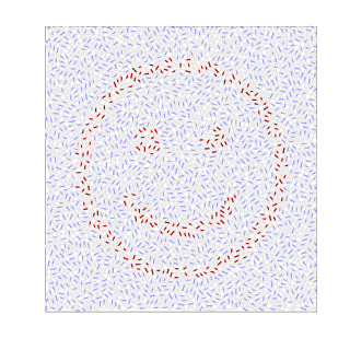
Figure 1: An example of training a “smiley” pattern. The red bonds are targets that are trained to have a stress, $t_{0}=10^{-3}$, blue bonds are trained to have a negative stress, $-t_{0}$ and the remaining grey bonds are the learning degrees of freedom. Here, the error is approximately $10^{-7}$.

Before turning to the training protocol, we first discuss physical constraints on the patterns a network can acquire.

Local constraints: A given node, with $z$ bonds, is in force balance when the sum of all forces equates to zero:

$$\sum_{b=1}^{z}t_{b}\hat{r_{b}}=0.$$ (1)

Here, $t_{b}$ are the tensions and $\hat{r_{b}}$ are the unit vectors of the bonds. When the tensions are small, the bond angles are fixed and the only degrees of freedom are the tensions on the bonds. Since there are $d$ equations for force balance the number of independent degrees of freedom are $z-d$. If the unit vectors are parallel then the number of independent degrees of freedom is reduced. While perfectly aligned bonds are non-generic, nearly parallel bonds can be found with a finite probability, which later we will argue leads to difficulties during training.

Global constraints: The tensions on the bonds in force balance, can decomposed in to a basis of states of self-stress(Lubensky et al., 2015). Recall, that the states self stress are the set of independent stresses that maintain force balance. The number of states of self-stress, $N_{sss},$ is related to the number of zero modes, $N_{z}$, the number of nodes, $N$, and the number of bonds, $N_{b}$ through the Maxwell-Calladine theorem(Maxwell, 1864; Calladine, 1978; Lubensky et al., 2015):

$$N_{sss}-N_{z}=N_{b}-dN.$$ (2)

Since the networks are rigid there are no zero modes, except for those that are contributed from the boundary conditions (translations and rotations). We neglect these in our count because their number is small with respect to the number of targets. Assuming the states of self-stress are extended, the maximal number of independent tensions that can be set is $N_{sss}$. We denote the number of target bonds per nodes as $\Delta=\frac{N_{T}}{N}$. The bound on the number of targets that can be trained, $\Delta_{c},$ is given by,

$$\Delta_{c}=\frac{N_{sss}}{N}\approx\frac{N_{b}}{N}-d=\frac{Z}{2}-d=\frac{\Delta Z}{2}.$$ (3)

This implies that highly coordinated network have a larger capacity and therefore we focus on this regime.

.3 Training protocol

Next we discuss the training protocol. As noted, there are two populations of bonds: target bonds, whose tension we aim to control, and the remaining bonds constitute the learning degrees of freedom; only these bonds change. We assume that their rest length evolves in proportion to tension on the bond, similar to a dashpot:

$$\partial_{t}\ell_{i,0}=\gamma k_{i}\left(\ell_{i}-\ell_{i,0}\right).$$ (4)

Our training protocol consists of alternating between two states. A free state where no external stresses are applied; in this state we only measure the stresses on the targets, denoted by, $t_{T}^{F}$. In the free state we also assume (for the time being) that the rest lengths do not change. We then switch to the clamped state and apply to the targets the clumped stresses, $t_{T}^{C}$. The applied clamped stresses are different that the desired stresses, $t_{T}^{D}$, and are chosen to evolve in proportion to the difference between the desired and free stresses,

$$\partial_{t}t_{T}^{C}=\lambda\left(t_{T}^{D}-t_{T}^{F}\right).$$ (5)

In the clamped state the rest lengths evolve, in accordance to Eq. 4, while in the free state we assume the system does not evolve. In experiment perhaps the free state can be frozen by either lowering the temperature, or spending very little time in the free state, so that the system changes very small.

The intuition behind this training rule is as follows. Imagine we begin in an unstressed state and squeeze a target bond to a desired $t_{T}^{D}$, while allowing the remaining bonds to evolve according to Eq. 4. Eventually, this causes the bonds to evolve to a state with no internal stress except on the squeezed target bond. When the targets are unclumped the system cannot return to the initial unstressed state. The stress on the target bond in the free state is then given by $t_{T}^{F}=\alpha t_{T}^{D}$, where $\alpha<1$. To achieve the desired stress we need to increase the value of the applied clumped stress, $t_{T}^{C}>t_{T}^{D}$. In essence, this protocol can be considered a control loop where the training signal integrates over the error.

We note that $\gamma$ defines a relaxation rate of the internal stresses. In our simulations we do not wait until the system completely relaxes in the clamped state(Stern et al., 2022). At each time step we compute the stresses in the free and clumped state by in force balance (by minimizing the energy), and evolve the rest length and clumped stresses in a single iteration of Eq. 4 and 5. Note that there are many choices for parameters which appear to have a weak effect on our results. In the data we present the parameters are as follows. The system is two dimensional with, $N=200$, $\lambda\Delta t=0.1$, $\gamma\Delta t=0.1$ (here, $\Delta t$ is the time step), and all the spring constants are identical taken to be $k_{i}=1.0$.

.4 Results

Next, we study numerically the success of our training rule. We define an error which sums over the all the target bonds and is normalized by the amplitude of the tension:

$$\eta=\frac{1}{t_{0}}\sqrt{\frac{1}{N_{T}}\sum_{i=1}^{N_{T}}\left(t_{T,i}^{D}-t_{T,i}^{F}\right)^{2}}.$$ (6)

We will consider two local selection rules for choosing the targets. First, we allow each node to have at most one target bond and later on we will consider having at most two target bonds per node. The number of targets on a given node affects the ease of training, and the possible resulting frustration.

Fig. 2(a) shows the error as a function of the number of cycles when each node has at most one target. At large times the decay is approximately exponential, and its decay is limited by computer precision. Increasing the number of targets yields slower convergence. We estimate the convergence time by measuring when the the error decreases to a given arbitrary value, $\eta=10^{-3}$. Fig. (b) shows the convergence time grows faster than a power-law. This could suggest a divergence at a finite value of $\Delta=\frac{N_{T}}{N}$, corresponding to a phase transition. The number of targets are limited by the requirement that each node has at most one target bond, and therefore we are unable to approach that transition.

We also consider the strength of the training stresses. Fig. 2(c) shows the root mean square of the clumped tensions,

$$\overline{t_{T}^{C}}=\sqrt{\frac{1}{N_{T}}\sum_{i=1}^{N_{T}}\left(t_{T,i}^{C}\right)^{2}}.$$ (7)

Initially, the training stresses grow with the number of training cycles and then reach a plateau. The plateau value increase with $\Delta$, and for the largest considered value, $\overline{t_{T}^{C}}\approx 10t_{0}$. Fig. 2(d) shows that the tension, similar to relaxation time grows faster than a power-law, again hinting at a possible inaccessible transition.

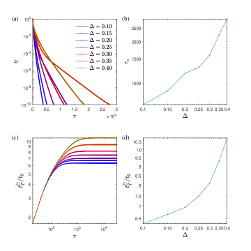
Figure 2: Training when each node has at most one target bond. (a) The error as a function of time for different numbers of targets. (b) The convergence time, defined by the number of cycles needed to reach $\eta=10^{-3}$, grows with $\Delta$. (c) The training forces in the clumped state as a function of time. (d) The training forces in the plateau as a function of the number of targets.

Next we consider the effect of allowing two target bonds per node. Fig. 3(a) shows the error as a function of number of cycles. As shown, the error decreases even for a large number of targets close to the maximal capacity, $\Delta_{c}\approx 0.75$. Unlike the case that each node had at most a single target bond, convergence does not appear to be exponential. A power-law fits reasonably at intermediate times. The difference in convergence is also expressed in the applied training tensions, $\overline{t_{T}^{C}}$. Fig 3(b) shows that the clumped tensions, $\overline{t_{T}^{C}}$, grow monotonically and do not appear to converge. Continual growth, we argue, is a mechanism that leads to failure at very large times. Therefore, it preferable to cease training after a finite number of cycles.

To study failure we increase $t_{0}$ and characterize how the system fails. Fig. 4(a) shows an example where the error initially decreases and then begins to steadily increase. The crossover time between these two regimes decreases upon increasing $t_{0}$. Namely, training with a small $t_{0}$ is more successful and failure occurs at much later times. Even though training fails on average, the majority of realizations are successful. Fig. 4(b) shows the fraction of realizations that failed, defined by $\eta>0.1$. The fraction of realizations that fail is fairly small, and increases with $t_{0}$. We also show in Fig. 4(c) that failure is accompanied by a sharp increase in the training tensions.

To identify how the system fails we have looked at videos of the dynamics. An example is presented in the supplementary information; here we present a single frame in Fig. 4(d). The learning degrees of freedom (bonds that are not targets) are plotted in grey. Targets whose error is small are dark, while blue bonds correspond to bonds whose tension is below the desired value and red are above the desired value. In Fig. 4(d) we show that the error is largest at a node where a blue and red bond meet at nearly $180^{o}$. The two bond have conflicting goals – one bond would like to increase the tension while the other would like to decrease the tension. This conflict causes the training forces on tensions to continually grow.

In Fig. 4(d) we also show in green the network in the clumped state. In the regime where $t_{0}$ is small, and when training is successful the clumped stresses are small. Therefore, the structure of the clumped state is nearly identical to that of the free state. However, due to the large forces induced by frustration the structure of the clumped state becomes very different from the free state. Thus, the geometry of the clumped state do not represent that of the free state, which contributes to failure.

In summary, having more than single bond per node may lead to frustration, which results in the training stresses continually growing and possibly failure. The frustrated nodes appear to be localized and somewhat rare but have an overwhelming contribution to the success of training. This suggests that the physics of rare regions is important(Vojta, 2006). This picture explains why having a very small $t_{0}$ is beneficial for training. Small $t_{0}$ allows for the structure in the clumped state to be similar to that of the free state even when the clumped tensions are multiples of $t_{0}$.

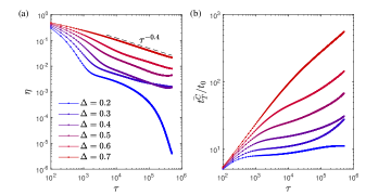
Figure 3: Training when each node has at most two target bonds. (a) The training error as function of time converges slower for large $\Delta$. Note, that the training error decreases even near the theoretical limit of $\Delta_{c}\approx 0.75$. (b) The training stresses as a function of time. Here, $t_{0}=10^{-6}.$

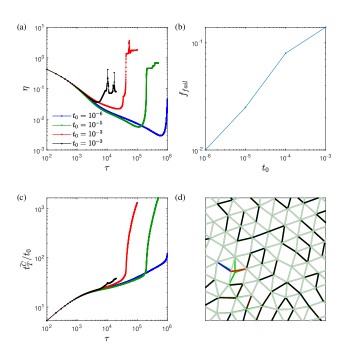
Figure 4: Analysis for failure to train when each node has at most two target bonds. (a) The error as a function of time. (b) The fraction of failed states as a function of $t_{0}$, define by $\eta>0.1$. (c) The training stresses as a function of time grow sharply when the error increases. (d) An example of a realization that failed in the free state. Two opposing target bonds, where the stress on one bond falls below the desired (blue) value while on second it is above the desired value (red). In green, the network in the clumped state differs from the network in the free state. Here, $t_{0}=10^{-4}.$

.5 Permanent memories

In the previous analysis we relied on the system having two states. A clumped state where each bond evolves in accordance to the stress on the bond and the free state which does not evolve. In principle, if the system is allowed to evolve in the free state all the stresses will decay to zero. To allow permanent memories, we consider dashpots with a yielding stress. That is, their rest length changes when the tension, $t_{i}$, exceeds a threshold value, $t_{th}$,

$$\partial_{t}\ell_{0,i}=\begin{cases}\gamma\left(t_{i}-t_{th}\right)&t>t_{th}\\ \gamma\left(t_{i}+t_{th}\right)&t<-t_{th}\\ 0&-t_{th}<t_{i}<t_{th}\end{cases}.$$ (8)

To allow for permanent memories the threshold must exceed the tension amplitude, $t_{0}$. In our simulations we take $t_{th}=2t_{0}$.

Here, we avoid frustration effects by allowing each node to have at most one target site. We first, consider the effect of the yielding stress when the network does not evolve in the free state. Fig. 5(a) shows the error as a function of time. Unlike the previous exponential decay, here, convergence is a power-law, $\eta\propto\tau^{\approx-1.0}$. The convergence of the error demonstrates the robustness of our results. We also measure the fraction of bonds that change their length at a given time, shown in Fig. 5(b). Here, only a small number of bonds, of order $N_{T}$, are affected by training at any given time.

The slow relaxation can be understood through a simple argument. Imagine that during training the stress on a target bond overshoots beyond the desired value. To undo this error the applied stress, $t_{T}^{C}$, must be reversed. However, to reverse the change in the rest length the applied tensions must be reversed by at least $t_{th}$. Since the rate of change to $t_{T}^{C}$ is proportional to the error, the time scale for reversing $t_{T}^{C}$ scales as $\tau\approx t_{c}/\eta$. Therefore, the error also decreases as $\eta\propto 1/\tau$.

Lastly, we relax our assumption that the free state does not evolve. We use the same rule, given in Eq. 8, for the free and clumped state and we allow the system to remain in the free and clumped state for equal periods of time. Fig. 5(c) shows the error as a function of time during training. Also here training is slow to converge. At the end of the training period we then allow the system to continually evolve in the free state, until all the tensions fall below $t_{th}$. Fig. 5(d) compares the error when training is complete and after the system is allowed to completely relax. After relaxation the error is slightly larger but overall still small. Since the system has completely relaxed in a frozen state ($\left|t_{i}\right|<t_{th}$) the trained patterns are permanent.

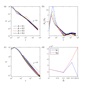
Figure 5: Training with dashpots that have a yield stress. (a) The error as function of time when the network evolves only in the clumped state is approximately a power-law. (b) The number of bonds that evolve in a given cycle is of order $N_{T}$. (c) The error as a function of time when the network evolves in both the clumped and free state is also approximately a power-law. (d) After the system has been trained we allow the system to relax in the free state. A comparison of the error before, $\eta_{C}$, and after the system has completly relaxed in the free state, $\eta_{R}$.

.6 Conclusions

In summary we have shown that a generic network of springs can be trained to encode a pattern of stresses at randomly selected target sites. We have introduced a training (learning) rule where the learning degrees are the rest lengths of the bonds, which evolve in proportion to the tension on the bond. The difference between the stresses in the free state and the desired stresses determine the change in training stresses in the clumped state. This training rule is robust and functions well even when the dashpots have a yielding stress, which allows to encode permanent memories.

We remark that our rule is different than the recent equilibrium propagation(Scellier and Bengio, 2017; Stern et al., 2020; Kendall et al., 2020; Stern et al., 2021; Anisetti et al., 2022) or the coupled learning(Stern et al., 2021). Those algorithm evolve as a function of the difference between the free and clumped state. In our case, the system evolves only in the clumped state, though the applied training stresses depend on measurements in the free state. We argue that our rule is advantageous, since the physical plasticity law depends only on the current state of the system.

We have also considered the convergence under different scenarios. We find that convergence depends on the local selection rule of the targets. When each node has at most a single target, convergence of the ordinary dashpots is exponential with a time scale that increases with the number of targets. For the dashpots with yielding stresses, convergence is approximately a power-law. Having two targets bonds per node also results in local frustration. Failure may occur when the training stresses grow without a bounded.

Our study presents another example of trainable materials. It is interesting to note that the same physical system of springs and dashpots was previously used to train strain responses. This demonstrates that different training rules allow to achieve for the same system different behaviors. Perhaps our training method could be useful in various applications, such as, creating optical patterns in photoelastic materials, designing materials with specific failure modes and possibly useful in manipulating flow networks.

.7 Appendix

Here we compute the convergence rate for two springs connected in series, where one of the springs is the target and the second spring is the learning degree of freedom. We consider two cases: 1. The system fully relaxes in the clumped state. That is, at each training cycle the rest lengths evolve in the clumped state until the tensions on the bonds vanish. 2. Finite relaxation rate. We assume that the overall length of the two springs is constrained to be , $L=\ell_{1}+\ell_{2}$, where $\ell_{i}$ denotes length of the bond. The two spring constants are taken to be equal, $k$. As above, the rest length of the target spring, $\ell_{1,0}$ does not change while the rest length of $\ell_{2,0}$ evolves as a function of the stress on that bond in the clumped state. The superscript $C,F$ denote the clumped and free state respectively.

.7.1 Complete relaxation

We begin by writing the tensions in the free state.

$$t_{1}^{F} =\frac{k}{2}\left(L-\ell_{1,0}-\ell_{2,0}\right).$$ (9)

Next we write the force balance equations in the clumped state:

$$k\left(\ell_{1}^{C}-\ell_{1,0}\right) =k\left(\ell_{2}^{C}-\ell_{2,0}\right)+t_{T}^{C},$$

where $t_{T}^{C}$ is the training stresses in the clamped state. Assuming complete relaxation in the clumped state we can set the tension on bond 2 to zero.

$$k\left(\ell_{1}^{C}-\ell_{1,0}\right) =t_{T}^{C}$$

$$\Rightarrow\ell_{2,0}= \ell_{2}^{C}=L-\ell_{1}^{C}=L-\ell_{1,0}-t_{T}^{C}/k$$

We can now express $t_{1}^{F}$ in terms of $t_{T}^{C}:$

$$t_{1}^{F} =\frac{t_{T}^{C}}{2}$$

Finally, the training rule evolves the clumped tension in accordance with,

$$\frac{d}{dt}t_{T}^{C} =\lambda\left(t_{0}-t_{1}^{F}\right)$$

$$=\lambda\left(t_{0}-\frac{t_{T}^{C}}{2}\right)$$

Convergence is therefore exponential with the rate constant given by $\lambda/2$,

$$t_{T}^{C}=2t_{0}+Ae^{-\frac{\lambda}{2}t}.$$

.7.2 Finite relaxation rate

Next we allow the rest length to evolve at a finite rate. As before, we solve the force balance equations, however, now without assuming that the force on the second bond vanishes. First we solve for $\ell_{2}^{C}$:

$$k\left(\ell_{1}^{C}-\ell_{1,0}\right) =k\left(\ell_{2}^{C}-\ell_{2,0}\right)+t_{T}^{C}$$

$$\Rightarrow\ell_{2}^{C} =\frac{1}{2}\left[-t_{T}^{C}/k+L-\ell_{1,0}+\ell_{2,0}\right]$$

The rest length of the second bond evolves via,

$$\frac{d\ell_{2,0}}{dt} =\gamma k\left(\ell_{2}^{C}-\ell_{2,0}\right)$$

$$=\frac{\gamma}{2}\left[-t_{T}^{C}/k+L-\ell_{1,0}-\ell_{2,0}\right]$$

$$=\gamma/k\left[-\frac{t_{T}^{C}}{2}+t_{1}^{F}\right]$$ (10)

Note, that in the last step we have plugged in Eq. 9. This equation can be recast in terms of $t_{1}^{F}:$

$$\frac{d}{dt}t_{1}^{F} =-\frac{k}{2}\ell_{2,0}=\frac{\gamma}{2}\left[\frac{t^{C}}{2}-t_{1}^{F}\right]$$

The evolution of $t_{T}^{C}$is therefore given by,

$$\frac{d}{dt}t_{T}^{C} =\lambda\left(t_{0}-t_{1}^{F}\right)$$ (11)

We must solve the two coupled equations Eq. 10 and 11. To this end we expressed these equation in matrix form,

$$\frac{d}{dt}\left(\begin{array}[]{c}t_{1}^{F}\\ t_{T}^{C}\end{array}\right)=\left(\begin{array}[]{cc}-\frac{\gamma}{2}&\frac{\gamma}{4}\\ -\lambda&0\end{array}\right)\left(\begin{array}[]{c}t_{1}^{F}\\ t_{T}^{C}\end{array}\right)+\left(\begin{array}[]{c}0\\ \lambda t_{0}\end{array}\right)$$

To solve for the relaxation rate we compute the two eigenvalues:

$$\mu_{1,2} =\frac{-\frac{\gamma}{2}\pm\sqrt{\left(\frac{\gamma}{2}\right)^{2}-\lambda\gamma}}{2}.$$

When, $\gamma-4\lambda>0$ convergence is exponential. When $\gamma-4\lambda<0$ there is also an oscillatory contribution. To ensure that our result is consistent with the case of full relaxation we take $\lambda/\gamma$ to be small, and expand the eigenvalues in a Taylor series:

$$\mu_{1} \approx-\frac{\gamma}{2}$$

$$\mu_{2} \approx-\frac{\lambda}{2}$$

Since convergence depends on the smaller eigenvalue, $\lambda$, our results are consistent with the case of complete relaxation.

References

- Anisetti et al. (2022) Anisetti, V. R., B. Scellier, and J. Schwarz (2022), arXiv preprint arXiv:2203.12098 .
- Bhattacharyya et al. (2022) Bhattacharyya, K., D. Zwicker, and K. Alim (2022), Physical Review Letters 129 (2), 028101.
- Calladine (1978) Calladine, C. (1978), International Journal of Solids and Structures 14, 161.
- Dillavou et al. (2022) Dillavou, S., M. Stern, A. J. Liu, and D. J. Durian (2022), Physical Review Applied 18 (1), 014040.
- Goodrich et al. (2015) Goodrich, C. P., A. J. Liu, and S. R. Nagel (2015), Physical review letters 114 (22), 225501.
- Hagh et al. (2022) Hagh, V. F., S. R. Nagel, A. J. Liu, M. L. Manning, and E. I. Corwin (2022), Proceedings of the National Academy of Sciences 119 (19), e2117622119.
- Hexner et al. (2020) Hexner, D., A. J. Liu, and S. R. Nagel (2020), Proceedings of the National Academy of Sciences 117 (50), 31690.
- Kendall et al. (2020) Kendall, J., R. Pantone, K. Manickavasagam, Y. Bengio, and B. Scellier (2020), arXiv preprint arXiv:2006.01981 .
- Lubensky et al. (2015) Lubensky, T. C., C. L. Kane, X. Mao, A. Souslov, and K. Sun (2015), Reports on Progress in Physics 78 (7), 073901.
- Maxwell (1864) Maxwell, J. C. (1864), The London, Edinburgh, and Dublin Philosophical Magazine and Journal of Science 27 (182), 294.
- Note1 (????) Previous studies on training found that the particular ensemble is unimportant.
- Note2 (????) In the appendix we compute the convergence rate for a simple case.
- O’Hern et al. (2003) O’Hern, C. S., L. E. Silbert, A. J. Liu, and S. R. Nagel (2003), Phys. Rev. E 68, 011306.
- Pashine et al. (2019) Pashine, N., D. Hexner, A. J. Liu, and S. R. Nagel (2019), Science advances 5 (12), eaax4215.
- Pisanty et al. (2021) Pisanty, B., E. C. Oğuz, C. Nisoli, and Y. Shokef (2021), SciPost Physics 10 (6), 136.
- Rocks et al. (2019) Rocks, J. W., H. Ronellenfitsch, A. J. Liu, S. R. Nagel, and E. Katifori (2019), Proceedings of the National Academy of Sciences 116 (7), 2506.
- Sartor and Corwin (2022) Sartor, J. D., and E. I. Corwin (2022), Physical Review Letters 129 (18), 188001.
- Scellier and Bengio (2017) Scellier, B., and Y. Bengio (2017), Frontiers in computational neuroscience 11, 24.
- Stern et al. (2020) Stern, M., C. Arinze, L. Perez, S. E. Palmer, and A. Murugan (2020), Proceedings of the National Academy of Sciences 117 (26), 14843.
- Stern et al. (2022) Stern, M., S. Dillavou, M. Z. Miskin, D. J. Durian, and A. J. Liu (2022), Physical Review Research 4 (2), L022037.
- Stern et al. (2021) Stern, M., D. Hexner, J. W. Rocks, and A. J. Liu (2021), Physical Review X 11 (2), 021045.
- Vojta (2006) Vojta, T. (2006), Journal of Physics A: Mathematical and General 39 (22), R143.
- Whitesides and Grzybowski (2002) Whitesides, G. M., and B. Grzybowski (2002), Science 295 (5564), 2418.