Real circles tangent to 3 conics

Abstract.

In this paper we study circles tangent to conics. We show there are generically $184$ complex circles tangent to three conics in the plane and we characterize the real discriminant of the corresponding polynomial system. We give an explicit example of $3$ conics with $136$ real circles tangent to them. We conjecture that 136 is the maximal number of real circles. Furthermore, we implement a hill-climbing algorithm to find instances of conics with many real circles, and we introduce a machine learning model that, given three real conics, predicts the number of circles tangent to these three conics.

1. Introduction

Problems of tangency have been of interest since early geometry. Apollonius, in the $`E\pi\alpha\phi\alpha\acute{\iota}$ (Tangencies), asked the following question: Given three circles in the plane, how many circles are tangent to all three? He showed that the answer is 8 in general. In $1848$ Steiner asked the related question of how many conics are tangent to five generic conics. Steiner conjectured that there are $6^{5}$ such conics, meeting the Bézout bound of the corresponding polynomial system. In $1859$ and $1864$ Jonquières and then Chasles established the correct answer of $3264$. In this paper we study a problem which sits in between:

Question 1.1.

Given three general conics $Q_{1},Q_{2},Q_{3}\subseteq\mathbb{C}^{2}$, how many circles are tangent to all three conics?

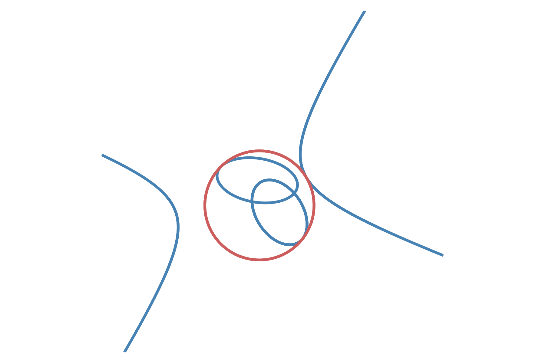
Figure 1. A red circle tangent to one blue hyperbola and two blue ellipses.

Circles are defined by three numbers – the coordinates of the center and the radius. Thus, we expect that the answer to our question is a finite number. Indeed, Emiris and Tzoumas [13] showed that there are at most 184 circles tangent to three general conics. We show in the next section that this bound is attained for generic conics.

Next, we turn our attention to the real version of 1.1. By a real conic we mean a conic whose defining equation has real coefficients. For three real circles the 8 Appolonius circles are real circles. The real version of Steiner's problem was studied only recently. In [19] the authors prove that there exist five real conics such that all $3264$ conics tangent to them are real. In [6], the authors use numerical algebraic geometry to explicitly find such an instance and compute all $3264$ real conics. Such arrangements are called fully real. In the same spirit we pose the following question.

Question 1.2.

Given three general real conics $Q_{1},Q_{2},Q_{3}\subseteq\mathbb{R}^{2}$, how many real circles are tangent to all three conics?

Here, we have the following result.

Theorem 1.3.

There is an instance of three real conics $Q_{1},Q_{2},Q_{3}\subseteq\mathbb{R}^{2}$, such that there are 136 real circles tangent to these three conics.

1.2 is much more subtle than 1.1. Of course, the answer to 1.1 gives an upper bound to 1.2 but it is non-trivial to verify whether or not that upper bound is tight. In fact, we are not able to prove that 136 is the maximal number. In [19] the authors show that a fully real instance of Steiner' conic problem exist in a neighborhood of the degenerate case where all five conics are double lines and each line intersects in the vertex of a regular pentagon. If we make the same construction for our circle problem, we find a maximum of $136$ real tritangent circles, not 184. The reason is that there are $4$ real conics that are tangent to $2$ lines and pass through $3$ points, but only $2$ real circles that are tangent to $2$ lines and pass through $1$ point [2] (circles are conics which pass through the two special circular points $\circ_{+}:=[1:i:0],\circ_{-}:=[1:-i:0]$ in $\mathbb{P}^{2}_{\mathbb{C}}$; see Equation 2.3). This discrepancy is the reason why we get 136 instead of 184 real circles using the strategy from [19]. This and computational evidence leads us to state the following conjecture.

Conjecture 1.4.

The maximal number of real circles tangent to three conics is 136.

As a first step towards proving 1.4 we give insight to 1.2 by characterizing the real discriminant of our tangency problem.

In the last part of the paper we approach 1.2 computationally. In Section 3 we implement a hill climbing algorithm, described in [10], to find explicit conics that have many real tritangent circles. For instance, we use the algorithm to find for every even number $0\leq n\leq 136$ an arrangement of conics such they have exactly $n$ real tritangent circles; see Theorem 3.1. In addition, we introduce a machine learning model that, given three real conics $Q_{1},Q_{2},Q_{3}$, predicts the number of real circles tangent to these conics. We do this using supervised learning on training data generated with the help of the hill climbing algorithm.

Our code and all the data we generated is available on our MathRepo page

https://mathrepo.mis.mpg.de/circlesTangentConics

1.1. Outline of paper

In Section 2 we answer 1.1 by showing that for three general conics there are $184$ tritangent complex circles. We then classify the real discriminant of our tangency problem and show that there exists conics that have $136$ real tritangent circles. Section 3 outlines the hill-climbing algorithm, while Section 4 explores the application of machine learning to predicting the real solution count.

1.2. Acknowledgements

We thank Taylor Brysiewicz for explaining to us the basic principles of the hill climbing algorithm in Section 3. We also thank Guido Montúfar, Rainer Sinn, and Bernd Sturmfels for helpful conversations.

Breiding is funded by the Deutsche Forschungsgemeinschaft (DFG, German Research Foundation) – Projektnummer 445466444.

Ong thanks Bowdoin College for support.

This project was initiated in an REU program organized by Rainer Sinn at the MPI MiS Leipzig. We thank MPI MiS for providing space for collaboration.

2. Real and complex circles tangent to three general conics

We begin by outlining the problem formulation under consideration. We work in an affine chart of $\mathbb{P}^{2}_{\mathbb{C}}$ that we identify with $\mathbb{C}^{2}$. Recall that a conic in the plane is the set of $(x,y)\in\mathbb{C}^{2}$ satisfying the equation:

(2.1) $$Q(x,y)=ax^{2}+bxy+cy^{2}+dx+ey+f=0$$

where $a,b,c,d,e,f\in\mathbb{C}$ and a circle of radius $r$ centered at $(s,t)\in\mathbb{C}^{2}$ is given by $(x,y)\in\mathbb{C}^{2}$ that satisfy:

$$C(x,y)=(x-s)^{2}+(y-t)^{2}-r^{2}=0.$$

The conic and circle intersect in 4 points, counting multiplicity and including points at infinity, so long as $Q$ and $C$ are irreducible and distinct. A point $(x,y)\in\mathbb{C}^{2}$ satisfying the two equations $Q(x,y)=C(x,y)=0$ is a point of tangency if and only if it has multiplicity at least two, or equivalently that the determinant of the Jacobian of $Q$ and $C$ vanishes:

$$\det\big{(}[\nabla Q(x,y)\ \ \nabla C(x,y)]\big{)}=0.$$

Here, $\nabla Q(x.y)=(\tfrac{\partial Q}{\partial x},\ \tfrac{\partial Q}{\partial y})^{T}$ denotes the gradient of $Q$. We denote this as

$$\nabla Q(x,y)\wedge\nabla C(x,y):=\det\big{(}[\nabla Q(x,y)\ \ \nabla C(x,y)]\big{)}.$$

This allows us to rephrase the tritangent circles problem as the set of solutions of a polynomial system. Let fix three conics

$$Q_{1}(x,y) =a_{1}x^{2}+a_{2}xy+a_{3}y^{2}+a_{4}x+a_{5}y+a_{6}$$

$$Q_{2}(x,y) =b_{1}x^{2}+b_{2}xy+b_{3}y^{2}+b_{4}x+b_{5}y+b_{6}$$

$$Q_{3}(x,y) =c_{1}x^{2}+c_{2}xy+c_{3}y^{2}+c_{4}x+c_{5}y+c_{6}$$

Let $(u_{i},v_{i})$ be the points of tangency on $Q_{i}$ (defined by $f_{1},f_{2},f_{3}$). A circle $C$ is tangent to all three of $Q_{1},Q_{2},Q_{3}$ if and only if the following conditions holds. First, $(u_{i},v_{i})\in Q_{i}$ for $1\leq i\leq 3$. This is formulated by the following three polynomials

$$f_{1} =a_{1}u_{1}^{2}+a_{2}u_{1}v_{1}+a_{3}v_{1}^{2}+a_{4}u_{1}+a_{5}v_{1}+a_{6}$$

$$f_{2} =b_{1}u_{2}^{2}+b_{2}u_{2}v_{2}+b_{3}v_{2}^{2}+b_{4}u_{2}+b_{5}v_{2}+b_{6}$$

$$f_{3} =c_{1}u_{3}^{2}+c_{2}u_{3}v_{3}+c_{3}v_{3}^{2}+c_{4}u_{3}+c_{5}v_{3}+c_{6}$$

Moreover, $(u_{i},v_{i})\in C$ for $1\leq i\leq 3$. For this we have again three polynomials

$$f_{4} =(u_{1}-s)^{2}+(v_{1}-t)^{2}-r^{2}$$

$$f_{5} =(u_{2}-s)^{2}+(v_{2}-t)^{2}-r^{2}$$

$$f_{6} =(u_{3}-s)^{2}+(v_{3}-t)^{2}-r^{2}$$

Finally, $\nabla Q_{i}(u_{i},v_{i})\wedge\nabla C(u_{i},v_{i})=0$ for $1\leq i\leq 3$, which is given by

$$f_{7} =2(u_{1}-s)(a_{2}u_{1}+2a_{3}v_{1}+a_{5})-2(v_{1}-t)(2a_{1}u_{1}+a_{2}v_{1}+a_{4})$$

$$f_{8} =2(u_{2}-s)(b_{2}u_{2}+2b_{3}v_{2}+b_{5})-2(v_{2}-t)(2b_{1}u_{2}+b_{2}v_{2}+b_{4})$$

$$f_{9} =2(u_{3}-s)(c_{2}u_{3}+2c_{3}v_{3}+c_{5})-2(v_{3}-t)(2c_{1}u_{3}+c_{2}v_{3}+c_{4})$$

These $3$ types of constraints define a parametrized polynomial system of equations

(2.2) $$F(x;p)=(f_{1},\dots,f_{9})^{T}=0$$

in the 9 variables $x=(u_{1},v_{1},u_{2},v_{2},u_{3},v_{3},s,t,r)$ and 18 parameters given by the coefficients of each conic $p=(a_{1},\ldots,a_{6},b_{1},\ldots,c_{6})$. For a fixed set of parameters $p$ defining three conics, a solution $x\in\mathbb{C}^{9}$ to the polynomial system $F(x;p)=0$ gives a circle with center $(s,t)$ and radius $r$ that are tangent to $Q_{1},Q_{2}$ and $Q_{3}$ at $(u_{1},v_{1}),\ldots,(u_{3},v_{3})$ respectively.

2.1. Complex circles tangent to three conics

We begin by answering 1.1. Observe that the Bézout bound of (2.2) is $2^{9}=512$ which is strict in this case, as [13] shows that there are at most $184$ circles tangent to three conics. We show this bound is attained for generic conics.

As in the case of Steiner's problem, the excess solutions arise in part from the locus of double lines. These double lines meet every conic at a point with multiplicity two, and are hence counted as tangent, regardless if the underlying reduced line is tangent or not.

Recall from Equation 2.1 that a conic is defined by 6 coefficients, so we can represent a conic by a point in $\mathbb{P}^{5}_{\mathbb{C}}$. The locus of double lines is then precisely the image of the map from $\mathbb{P}^{2}_{\mathbb{C}}$, the space of lines, to $\mathbb{P}^{5}_{\mathbb{C}}$ by

$$[a:b:c]\mapsto[a^{2}:2ab:b^{2}:ac:bc:c^{2}].$$

This is the Veronese embedding, which we denote $V$. We can eliminate this excess intersection by blowing up our space of conics along $V$. Denote $X:=\mathrm{Bl}_{V}(\mathbb{P}^{5}_{\mathbb{C}})$ the blowup of $\mathbb{P}^{5}_{\mathbb{C}}$ along the Veronese surface $V$ and $\pi:\mathrm{Bl}_{V}(\mathbb{P}^{5}_{\mathbb{C}})\to\mathbb{P}^{5}_{\mathbb{C}}$ the blowing down morphism. The algebraic variety $X$ is called the space of complete conics.

Fix a general point $p\in\mathbb{P}^{2}$, a general line $\ell\subset\mathbb{P}^{2}$ and a general conic $Q\subset\mathbb{P}^{2}$. Let $H_{p},H_{\ell},H_{Q}$ be the hypersurfaces in $\mathbb{P}^{5}_{\mathbb{C}}$ corresponding to conics that pass through $p$, are tangent to $\ell$, or tangent to $Q$, respectively. We denote by $\widetilde{H_{p}},\widetilde{H_{\ell}},\widetilde{H_{Q}}$ the classes of $\pi^{-1}(H_{p}),\pi^{-1}(H_{\ell}),\pi^{-1}(H_{Q})$ in the Chow ring of $X$; see, e.g., [12, Chapter 1] for more information on Chow rings and how they are used. Furthermore, we denote by $E$ the class of $\pi^{-1}(V)=E\subseteq X$, called exceptional divisor, away from which the blowing down map is an isomorphism of algebraic varieties.

Recall that we want to count the number of conics that fulfill some intersection conditions. This corresponds to counting the number of points in an algebraic set of dimension zero that is defined by the intersection of $\widetilde{H_{p}},\widetilde{H_{\ell}}$ and $\widetilde{H_{Q}}$ in $X$. The classes $\widetilde{H_{p}},\widetilde{H_{\ell}},\widetilde{H_{Q}}$ do not intersect in the exceptional divisor $E$; see, e.g., [15, p. 749-56]. This means that they meet transversely away from the subvariety of singular conics and have no common points in $E$. Thus any intersection problem involving conics, that contain a general point, or are tangent to a general line or a general conic, can be computed by taking the degree of the product of the corresponding classes in the Chow ring.

Let now $C\subseteq\mathbb{P}^{2}_{\mathbb{C}}$ be a circle. We can describe $C$ a circle with center $[s:t:r]$ and radius $r$ as the vanishing locus of the equation $(x-sz)^{2}+(y-tz)^{2}-r^{2}z^{2}\in\mathbb{C}[x,y,z]$. Note that $C$ passes through the circular points

(2.3) $$\circ_{+}:=[1:i:0]\quad\text{ and }\quad\circ_{-}:=[1:-i:0]$$

and conversely that any conic passing through $\circ_{+},\circ_{-}$ is in fact a circle. Circles, then, are conics that pass through the circular points $\circ_{+},\circ_{-}$. We wish to enumerate the number of circles mutually tangent to three conics. By the above, these are precisely the conics mutually tangent to three general conics that also pass through the two circular points. The number of circles tangent to three general conics are thus given by the intersection product $\widetilde{H_{Q}}^{3}\cdot\widetilde{H_{\circ_{+}}}\cdot\widetilde{H_{\circ_{-}}}$.

Emiris and Tzoumas [13] used this observation and computed the upper bound $\widetilde{H_{Q}}^{3}\cdot\widetilde{H_{p}}^{2}=184$, where $p$ is a general point in the sense of intersection theory (see also the survey article by Kleiman and Thorup [22]). A priori, it is not clear that taking $p$ to be the circular points $\circ_{+}$ or $\circ_{-}$ is general in the sense of intersection theory. Therefore, for completeness we give the full proof of the fact that the answer to 1.1 is 184.

Proposition 2.1.

Given three general conics $Q_{1},Q_{2},Q_{3}\subseteq\mathbb{C}^{2}$, there are 184 circles tangent to these three conics.

Proof.

We wish to compute $\widetilde{H_{Q}}^{3}\cdot\widetilde{H_{\circ_{+}}}\cdot\widetilde{H_{\circ_{-}}}$. We know that conics degenerate into flags, so the condition of being tangent to a conic $Q$ is equivalent to the condition that it contains either of two points or is tangent to either of two lines. This gives us the equality $\widetilde{H_{Q}}=2\widetilde{H_{p}}+2\widetilde{H_{\ell}}$; see also [15, p. 775].

We now seek to verify that $\widetilde{H_{p}}=\widetilde{H_{\circ_{+}}},\widetilde{H_{\circ_{-}}}$. To show this, it suffices to show that the 4-planes in $\mathbb{P}^{5}_{\mathbb{C}}$ defined by conics passing through either of $\circ_{+},\circ_{-}$ do not contain the Veronese $V$ or, equivalently, that the equation defining the 4-plane vanishes to order zero on $V$; see [11, p. 105]. But since the hypersurfaces $H_{\circ_{+}}$ and $H_{\circ_{-}}$ do not contain the Veronese, we know that are $\widetilde{H_{\circ_{-}}}=\widetilde{H_{p}}+0\cdot E=\widetilde{H_{p}}$ and, similarly, $\widetilde{H_{\circ_{+}}}=\widetilde{H_{p}}$. Namely the circular points $\circ_{+}$ and $\circ_{-}$ are general in the sense of intersection theory.

Using the two facts above, we can enumerate the number of circles tangent to three general conics as the number of conics tangent to three general conics and passing through two general points. This gives us

$$(2\widetilde{H_{p}}+2\widetilde{H_{\ell}})^{3}\cdot\widetilde{H_{\circ_{+}}}\cdot\widetilde{H_{\circ_{-}}} =(2\widetilde{H_{p}}+2\widetilde{H_{\ell}})^{3}\cdot\widetilde{H_{p}}^{2}$$

$$=8\cdot\widetilde{H_{p}}^{5}+24\cdot\widetilde{H_{p}}^{4}\cdot\widetilde{H_{\ell}}+24\cdot\widetilde{H_{p}}^{3}\cdot\widetilde{H_{\ell}}^{2}+8\cdot\widetilde{H_{p}}^{2}\cdot\widetilde{H_{\ell}}^{3}.$$

Over $\mathbb{P}^{2}_{\mathbb{C}}$ there is one conic through 5 general points $\widetilde{H_{p}}^{5}=1$, two conics through four general points and tangent to one general line $\widetilde{H_{p}}^{4}\cdot\widetilde{H_{\ell}}=2$, four conics through three general points and tangent to two general lines $\widetilde{H_{p}}^{3}\cdot\widetilde{H_{\ell}}^{2}=4$, and four conics through two general points and tangent to three general lines $\widetilde{H_{p}}^{2}\cdot\widetilde{H_{\ell}}^{3}=4$; see [12, p. 307]. Making the appropriate substitutions yields

$$8\cdot 1+24\cdot 2+24\cdot 4+8\cdot 4=184$$

which gives the claim. ∎

2.2. Real circles tangent to three conics

We now turn our attention to understanding to 1.2.

In the real version of Steiner's problem of finding the maximum number of real conics tangent to 5 general conics [19], the authors show that in a neighborhood of the corresponding real discriminant where all five conics are singular, there is an open cell where the number of real solutions achieves the complex upper bound. Using this same idea, we show that in our case this neighborhood produces at most $136$ real solutions. Notice that the following theorem, in particular, proves Theorem 2.2.

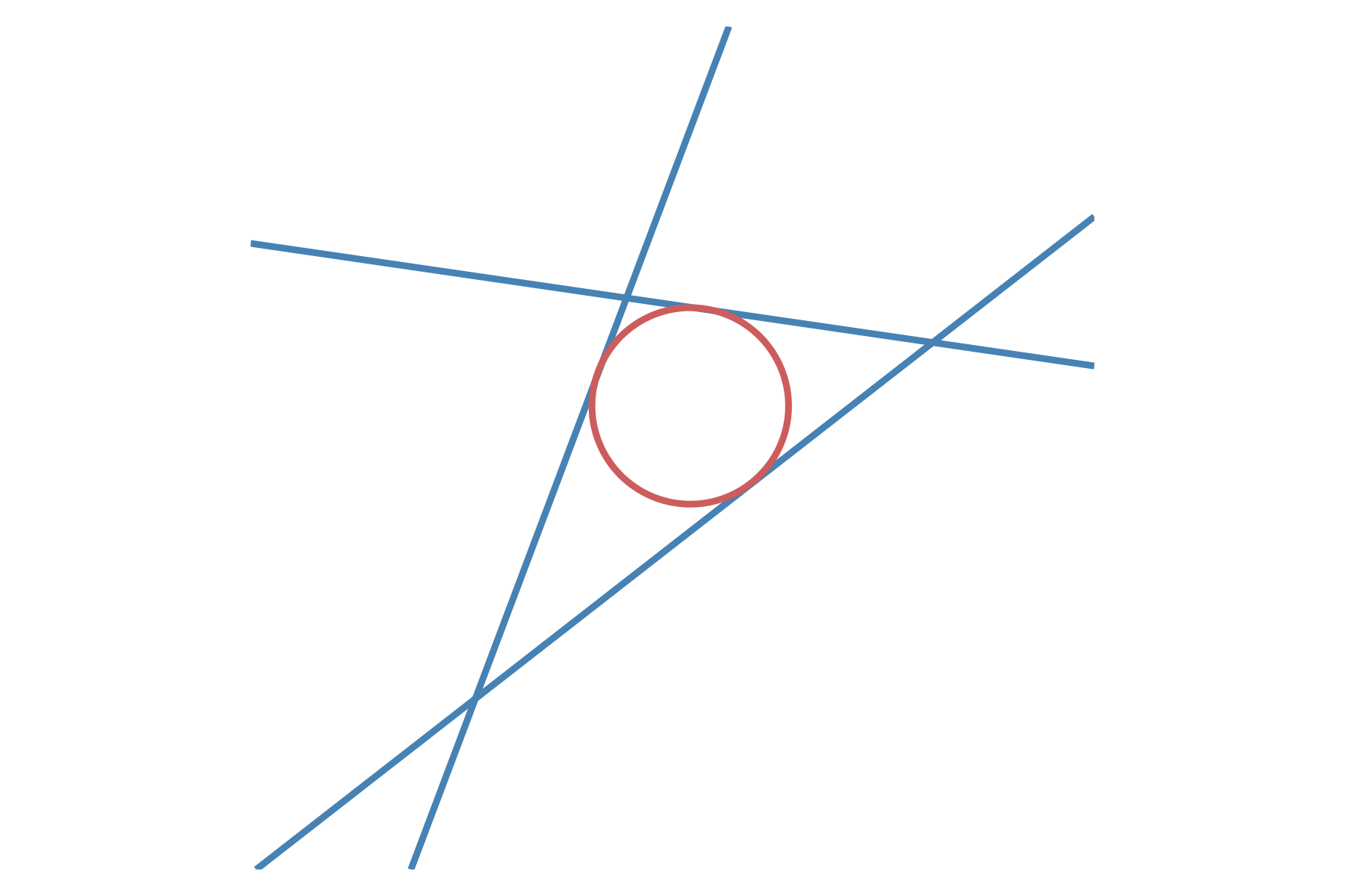
Figure 2. A red circle tangent to three blue lines that form a triangle. The proof of Theorem 2.2 considers such a triangle and finds a nearby arrangement of three hyperbolas, such that there are 136 real circles tangent to the three hyperbolas. In fact, the arrangement of hyperbolas in the proof of Theorem 1.3 is near the triangle shown in the picture.

Theorem 2.2.

Let $Q_{1},Q_{2},Q_{3}$ be three real conics in the plane such that $Q_{1},Q_{2},Q_{3}$ are all singular. There are at most $136$ real circles tangent to three conics in a neighborhood of $Q_{1},Q_{2},Q_{3}$.

Proof.

We adapt the argument of [19] as presented in [21, Ch. 7] of deforming a special configuration of conics. Suppose $\ell_{1},\ell_{2},\ell_{3}$ are lines supporting the edges of a triangle and $p_{i}\in\ell_{i}$ for $1\leq i\leq 3$ are points in the interior of the corresponding edge.

We consider a subset of the lines $S\subseteq\{\ell_{1},\ell_{2},\ell_{3}\}$ and a subset $P_{S}\subseteq\{p_{1},p_{2},p_{3}\}$ of the points, such that for all $p_{i}\in P_{S}$, $\ell_{i}\not\in S$. For every subset $S\subseteq\{\ell_{1},\ell_{2},\ell_{3}\}$ of the lines, there are

$$\widetilde{H_{\circ_{+}}}\cdot\widetilde{H_{\circ_{-}}}\cdot\widetilde{H_{\ell}}^{|S|}\cdot\widetilde{H_{p}}^{3-|S|}=2^{\,\min\{|S|-2,\ 3-|S|\}+2}$$

complex circles that are tangent to the lines in $S$ and meet the $3-|S|$ points in $P_{S}$. Figure 2 shows an example of a circle that is tangent to three lines (i.e., $|S|=3$).

Note, however, for $|S|=2$, there are $4=2^{2}$ complex but only $2$ real circles tangent to two lines and passing through a point [2]. Altogether, this gives

$$\sum_{k=0}^{3}2^{\,\min\{k-2,\ 3-k\}+2}\,\binom{3}{k}=1\cdot\binom{3}{0}+2\cdot\binom{3}{1}+4\cdot\binom{3}{2}+4\cdot\binom{3}{3}=23$$

complex circles, but only

$$1\cdot\binom{3}{0}+2\cdot\binom{3}{1}+2\cdot\binom{3}{2}+4\cdot\binom{3}{3}=17$$

real circles that for each $1\leq i\leq 3$ either meet $p_{i}$ or are tangent to $\ell_{i}$.

With an asymmetric configuration, exactly $17$ of the real circles meet each point $p_{i}$ and none of the $17$ tangent to $\ell_{i}$ are tangent at the point $p_{i}$. We now replace each pair $(p_{i},\ell_{i})$ with a smooth hyperbola $h_{i}$ that is asymptotically close to it: a hyperbola whose branches are close to $\ell_{i}$ and flex points close to $p_{i}$. If we do this for a pair $(p_{i},\ell_{i})$ then for every conic in our configuration there will be two nearby circles tangent to $h_{i}$ – one at each branch of the hyperbola. Replacing each pair $(p_{i},\ell_{i})$ by $h_{i}$ for $1\leq i\leq 3$, we get $2^{3}\cdot 17=136$ real circles, proving our claim. ∎

Theorem 2.2 implies Theorem 1.3. In the next section we give a constructive proof of Theorem 1.3.

2.3. The real discriminant

As a step towards the resolution of 1.4 we characterize the real discriminant of the polynomial system (2.2), whose solutions describe circles tangent to three conics.

The real discriminant $\Delta\subseteq\mathbb{R}^{18}$ of (2.2) is a hypersurface in the space of real parameters where the parameters $p=(a_{1},\ldots,a_{6},b_{1},\ldots,c_{6})\in\Delta$ if and only if the number of real circles tangent to the three real conics defined by $p$ is not locally constant. We call such real parameters and the corresponding arrangement of conics degenerate. In other words, $\Delta$ divides the parameter space $\mathbb{R}^{18}$ into open cells in which the number of real solutions to (2.2) is constant.

Theorem 2.3 (The real discriminant).

Let $\{i,j,k\}=\{1,2,3\}$. An arrangement of three real conics $Q_{1},Q_{2},Q_{3}$ is degenerate, if and only if one the following holds:

1. There is a real line tangent to $Q_{1},Q_{2},Q_{3}$.

2. $Q_{1},Q_{2}$ and $Q_{3}$ intersect in a real point.

3. $Q_{i}$ is singular at a real point $(u_{i},v_{i})$, and there is a real circle tangent to $Q_{j},Q_{k}$ that passes through $(u_{i},v_{i})$.

4. $Q_{i}$ and $Q_{j}$ meet tangentially in a real point.

5. There exists a real circle $C$ that is tangent to $Q_{1},Q_{2},Q_{3}$ at the real points $(u_{1},v_{1}),(u_{2},v_{2}),(u_{3},v_{3})$, respectively, and the curvature of $C$ equals the curvature of $Q_{i}$ at $(u_{i},v_{i})$ and the normal vectors $\nabla C(u_{i},v_{i})$ and $\nabla Q(u_{i},v_{i})$ point in the same direction.

Proof.

The discriminant consists of those real parameters $p\in\mathbb{R}^{18}$, where the polynomial system $F(x;p)=(f_{1}(x;p),\ldots,f_{9}(x;p))$ from Equation 2.2 has

1. a real solution at infinity.

2. a real solution $x\in\mathbb{R}^{9}$, such that the Jacobian matrix

   $$J_{x}=J_{x}(x;p)=\begin{bmatrix}\frac{\partial f_{1}(x;p)}{\partial x}&\ldots&\frac{\partial f_{9}(x;p)}{\partial x}\end{bmatrix}^{T}\in\mathbb{R}^{9\times 9}$$

   of $F$ at $x$ is singular.

Let us first consider when a real solution goes off to infinity. First note that circles have only two points at infinity, namely $[1:\pm i:0]$. These are non-real points, so not limits of real solutions. Therefore, in order to have a real solution go to infinity, we must have at least one of $(a,b,r)$ go to infinity. If $r$ goes to infinity then it is a circle of infinite radius, which has curvature $0$ so it is a line. If $r$ is bounded then the circle converges to either $(x-a)^{2}=0$ or $(y-b)^{2}=0$ or $(x-a)^{2}+(y-b)^{2}=0$. In any of these cases it is either a line or a point at infinity. Therefore, two real solutions go to infinity when there is a line tangent to all three conics, which proves the statement.

The rest of the proof consists of showing that cases (2)–(5) correspond exactly to those situation we the Jacobian matrix is singular.

If $r=0$, the three conics $Q_{1},Q_{2}$ and $Q_{3}$ must intersect in a point $(u,v)$ and we have the circle $(x-u)^{2}+(y-v)^{2}=0$ tangent to all three conics, which gives a singular solution to the system (2.2). This is the second item above. Therefore, in the following we assume that $r\neq 0$.

The polynomial system in (2.2) consists of three triplets of polynomials, namely:

$$\psi_{i}(u_{i},v_{i},a,b,r):=\begin{pmatrix}C(u_{i},v_{i})\\ Q_{i}(u_{i},v_{i})\\ \nabla C(u_{i},v_{i})\wedge\nabla Q_{i}(u_{i},v_{i})\end{pmatrix}\in\mathbb{R}^{3}\text{ for }i=1,2,3.$$

Let $J_{x}^{(i)}$ denote the Jacobian matrix of $\psi_{i}$ at $x$. Then,

(2.4) $$J_{x}=\begin{bmatrix}J_{x}^{(1)}\\ J_{x}^{(2)}\\ J_{x}^{(3)}\end{bmatrix}=\begin{bmatrix}A^{(1)}&0&0&B^{(1)}\\ 0&A^{(2)}&0&B^{(2)}\\ 0&0&A^{(3)}&B^{(3)},\end{bmatrix}$$

where $A^{(i)}\in\mathbb{R}^{3\times 2}$ contains the partial derivatives of $\psi_{i}$ with respect to $(u_{i},v_{i})$, and $B^{(i)}\in\mathbb{R}^{3\times 3}$ contains the partial derivatives of $\psi_{i}$ with respect to $a,b,r$.

We have $\nabla C(x,y)=2(x-a,y-b)^{T}$ and so

$$\frac{\partial\nabla C(u_{i},v_{i})}{\partial a}=\begin{pmatrix}-2\\ 0\end{pmatrix},\quad\frac{\partial\nabla C(u_{i},v_{i})}{\partial b}=\begin{pmatrix}0\\ -2\end{pmatrix},\quad\frac{\partial\nabla C(u_{i},v_{i})}{\partial r}=\begin{pmatrix}0\\ 0\end{pmatrix}.$$

This shows that for $(\dot{u}_{i},\dot{v}_{i},\dot{a},\dot{b},\dot{r})^{T}\in\mathbb{R}^{5}$ we have

(2.5) $$J_{x}^{(i)}\,\begin{pmatrix}\dot{u}_{i}\\ \dot{v}_{i}\\ \dot{a}\\ \dot{b}\\ \dot{r}\end{pmatrix} =A^{(i)}\,\begin{pmatrix}\dot{u}_{i}\\ \dot{v}_{i}\end{pmatrix}+B^{(i)}\,\begin{pmatrix}\dot{a}\\ \dot{b}\\ \dot{r}\end{pmatrix}$$

$$=\begin{pmatrix}2\begin{pmatrix}\dot{u}_{i}\\ \dot{v}_{i}\end{pmatrix}^{T}\nabla C(u_{i},v_{i})+\dot{C}(u_{i},v_{i})\\[3.00003pt] 2\begin{pmatrix}\dot{u}_{i}\\ \dot{v}_{i}\end{pmatrix}^{T}\nabla Q(u_{i},v_{i})\\[3.00003pt] 2\begin{pmatrix}\dot{u}_{i}-\dot{a}\\ \dot{v}_{i}-\dot{b}\end{pmatrix}\wedge\nabla Q_{i}(u_{i},v_{i})+\nabla C(u_{i},v_{i})\wedge\mathrm{H}(Q_{i})\begin{pmatrix}\dot{u}_{i}\\ \dot{v}_{i}\end{pmatrix},\end{pmatrix}$$

where $\dot{C}(x,y)=-2(x-a)\dot{a}-2(y-b)\dot{b}-2r\dot{r}$ and

$$\mathrm{H}(Q_{i})=\begin{bmatrix}\ \frac{\partial^{2}Q_{i}}{\partial^{2}u_{i}}\ &\ \frac{\partial^{2}Q_{i}}{\partial u_{i}\partial v_{i}}\ \\[5.0pt] \ \frac{\partial^{2}Q_{i}}{\partial u_{i}\partial v_{i}}\ &\ \frac{\partial^{2}Q_{i}}{\partial^{2}v_{i}}\ \end{bmatrix}$$

is the Hessian of $Q_{i}$ at $(u_{i},v_{i})$. Notice that $\dot{C}(x,y)$ is an affine linear function.

We have to show that the cases (3)–(5) above give exactly those situations, where we can find a nonzero vector $(\dot{u}_{i},\dot{v}_{i},\dot{a},\dot{b},\dot{r})^{T}\in\mathbb{R}^{5}$ such that the vector in (2.5) is equal to $0$ for each $i=1,2,3$. Since each of the equations is homogeneous in $u_{i},v_{i}$, we can assume that

(2.6) $$u_{1}^{2}+v_{1}^{2}=u_{2}^{2}+v_{2}^{2}=u_{3}^{2}+v_{3}^{2}=1.$$

If $Q_{i}$ is singular, we have a point $(u_{i},v_{i})$ with $Q_{i}(u_{i},v_{i})=0$ and $\nabla Q_{i}(u_{i},v_{i})=0$. The point $(u_{i},v_{i})$ is part of a solution $F(u_{1},\ldots,v_{3},a,b,r)=0$, if and only if there is a circle that is tangent to the other two conics $Q_{j}$ and $Q_{k}$ at $(u_{j},v_{j})$ and $(u_{k},v_{k})$, respectively, and that passes through $(u_{i},v_{i})$. For this data $J_{x}\,(\dot{u}_{i},\dot{v}_{i},\dot{a},\dot{b},\dot{r})^{T}=0$ becomes a system of $8$ linear equations in $9$ variables. This always has a nontrivial solution.

Next, since $C$ is tangent to $Q_{i}$ at $(u_{i},v_{i})$, we have $\nabla C(u_{i},v_{i})\wedge\nabla Q_{i}(u_{i},v_{i})=0$; i.e, $\nabla C(u_{i},v_{i})$ is a multiple of $\nabla Q(u_{i},v_{i})\neq 0$. The second entry in (2.5) then implies

$$\begin{pmatrix}\dot{u}_{i}\\ \dot{v}_{i}\end{pmatrix}^{T}\nabla C(u_{i},v_{i})=0,$$

so that $\dot{C}(u_{i},v_{i})=0$ by the first entry. Unless $\dot{C}=0$, this implies that the three points $(u_{1},v_{1}),(u_{2},v_{2}),(u_{3},v_{3})$ lie on a line. Since they also lie on the circle of positive radius $r>0$, this implies $(u_{i},v_{i})=(u_{j},v_{j})$ for at least one pair $i\neq j$. But then $Q_{i}$ and $Q_{j}$ intersect tangentially at $(u_{i},v_{i})$. In this case, in (2.4) we get $A^{(i)}=A^{(j)}$ and $B^{(i)}=B^{(j)}$, which gives a singular Jacobian $J_{x}$. This shows that item 4 above gives singular solutions.

So, outside the discriminant we must have $\dot{C}=0$; i.e., $\dot{a}=\dot{b}=\dot{r}=0$. Since $\psi_{i}$ does not depend on $(u_{j},v_{j})$ for $j\neq i$, this means in order to understand when $J_{x}$ is singular, it is now enough to study when the equations in (2.5) vanish. For $\dot{C}=0$ the third equation in (2.5) becomes

(2.7) $$2\begin{pmatrix}\dot{u}_{i}\\ \dot{v}_{i}\end{pmatrix}\wedge\nabla Q_{i}(u_{i},v_{i})-\mathrm{H}(Q_{i})\begin{pmatrix}\dot{u}_{i}\\ \dot{v}_{i}\end{pmatrix}\wedge\nabla C(u_{i},v_{i})=0.$$

We have $(\nabla C(u_{i},v_{i}))^{T}\nabla C(u_{i},v_{i})=4r^{2}>0$ and $(\nabla Q(u_{i},v_{i}))^{T}\nabla Q(u_{i},v_{i})>0$, since $Q_{i}$ is smooth. Then, multiplying (2.7) by $2r\sqrt{(\nabla Q(u_{i},v_{i}))^{T}\nabla Q(u_{i},v_{i})}$ and using (2.6) and the fact that

$$\begin{pmatrix}\dot{u}_{i}\\ \dot{v}_{i}\end{pmatrix}^{T}\nabla Q(u_{i},v_{i})=\begin{pmatrix}\dot{u}_{i}\\ \dot{v}_{i}\end{pmatrix}^{T}\nabla C(u_{i},v_{i})=0$$

we have

$$\frac{\varepsilon_{i}}{r}=\begin{pmatrix}\dot{u}_{i}\\ \dot{v}_{i}\end{pmatrix}^{T}\frac{\mathrm{H}(Q_{i})}{\sqrt{(\nabla Q(u_{i},v_{i}))^{T}\nabla Q(u_{i},v_{i})}}\begin{pmatrix}\dot{u}_{i}\\ \dot{v}_{i}\end{pmatrix},$$

where $\varepsilon_{i}=1$, if $\nabla Q(u_{i},v_{i})$ and $\nabla Q(u_{i},v_{i})$ point into the same direction, and $\varepsilon_{i}=-1$ otherwise. Since, $r^{-1}$ is the curvature of $C$ and the right hand side equals the curvature of $Q_{i}$ at $(u_{i},v_{i})$, this shows that we have a singular solution also in the fifth item above. In all other cases, $J_{x}$ has a trivial kernel, hence is not singular. ∎

3. Hill climbing

Theorem 2.2 shows that there exist three real conics that have 136 real circles tangent to all three, but it does not provide an explicit construction of the three conics. To find conics that exhibit this behavior, we rely on a numerical method known as hill climbing. We adapt a method of Dietmaier in [10] to increase the count of real solutions. For the ease of exposition, we outline our method below using matrix inverses. In our implementation we do not invert any matrices and instead we introduce auxiliary variables and solve an equivalent linear system, allowing for more numerically stable computations.

The basic idea of the hill climbing algorithm is as follows. Suppose we are given a set of parameters $p=(a_{1},\dots,a_{6},b_{1},\dots,c_{6})\in\mathbb{R}^{18}$ defining a configuration of three general conics in the plane. By 2.1, the system of polynomial equations $F(x;p)=0$ from (2.2) has 184 complex solutions. To increase the number of real solutions, we iteratively perturb $p$ so that a complex conjugate solution pair first becomes a double real root then perturb $p$ once again to separate this double root resulting in two distinct real roots. Simultaneously, we ensure that no existing real solution vectors become arbitrarily close, forming a double root and eventually a complex conjugate pair and that solutions do not diverge to infinity.

For fixed parameters $p\in\mathbb{R}^{18}$, denote $S$ by

$$S=S_{\mathbb{R}}\sqcup S_{\mathbb{C}}\subseteq\mathbb{C}^{9}$$

the solutions of our system of polynomial equations (2.2) where $S_{\mathbb{R}}$ is the set of solutions with only real entries and $S_{\mathbb{C}}=S\setminus S_{\mathbb{R}}$.

In the first step of the hill climbing algorithm, we select one solution $x^{*}\in S_{\mathbb{C}}$ in which we aim to decrease the $L^{1}$ norm $\|\mathrm{Im}(x^{*})\|_{1}$ of the vector of imaginary parts of $x^{*}$. The goal is to compute a step $\Delta p$ in the parameter space $\mathbb{R}^{18}$, such that the magnitude of the imaginary part of $x^{*}$ decreases as we move from $p$ to $p+\Delta p$ for some $-\varepsilon\mathbbm{1}\leq\Delta p\leq\varepsilon\mathbbm{1}$ where $\varepsilon$ is a small tolerance parameter and $\mathbbm{1}=(1,\ldots,1)^{T}\in\mathbb{R}^{18}$ is the all-one vector.

As in the previous section we denote by $J_{x}(x;p)\in\mathbb{C}^{9\times 9}$ the Jacobian matrix of $F(x;p)$ with respect to the variables $x=(u_{1},v_{1},\dots,s,t,r)$ evaluated at $x$ with parameters $p$. Similarly, $J_{p}(x;p)\in\mathbb{C}^{9\times 18}$ is the Jacobian of $F(x;p)$ with respect to the parameters $p=(a_{1},\dots,a_{6},b_{1},\dots,b_{6})$ evaluated at $x$ with parameters $p$. Following [10] we observe that differentiating both sides of $F(x;p)=0$ with respect to $p$ and $x$, gives the following matrix equation involving the step $\Delta p$:

(3.1) $$J_{x}(x;p)\Delta x+J_{p}(x;p)\Delta p=0.$$

Solving (3.1) for $\Delta x$, we have that

(3.2) $$\text{Im}(\Delta x)=-\text{Im}(J_{x}(x;p)^{-1}\cdot J_{p}(x;p))\cdot\Delta p,$$

where $\text{Im}(\cdot)$ denotes taking the componentwise imaginary part. Let $\text{sign}(\cdot)$ denote the componentwise sign function. In order to decrease $\lVert\Delta\text{Im}(x^{*})\rVert_{1}$, we wish to minimize

$$-\text{sign}(\text{Im}(x^{*}))^{T}\cdot\text{Im}(J_{x}(x^{*};p)^{-1}\cdot J_{p}(x^{*};p))\cdot\Delta p.$$

Notice that this objective function considers a first order approximation of our system $F(x,p)$ at $(x^{*},p)$, so we add the constraint $-\varepsilon\mathbbm{1}\leq\Delta p\leq\varepsilon\mathbbm{1}$ to ensure that this approximation is accurate enough.

Next, we want to ensure that as we take a step in the parameter space, two existing real solutions do not come together to become non-real. Consider two real solutions $x_{i},x_{j}\in S_{\mathbb{R}}$. The distance between $x_{i},x_{j}$ is the $L^{2}$ norm $D=\lVert x_{i}-x_{j}\rVert_{2}^{2}$. Differentiating $D$ with respect to $x$ yields

$$2\cdot\langle x_{i}-x_{j},\Delta x_{i}-\Delta x_{j}\rangle.$$

Substituting (3.2) in for $\Delta x_{i},\Delta x_{j}$, we have an expression that gives the change in the distance between two real solutions $x_{i},x_{j}$ as a function of the change in parameters. Since we do not want this distance to decrease, we impose the constraint

$$\forall x_{i},x_{j}\in S_{\mathbb{R}}:(x_{i}-x_{j})^{T}\cdot\big{(}J_{x}(x_{i};p)^{-1}\cdot J_{p}(x_{i};p)-J_{x}(x_{j};p)^{-1}\cdot J_{p}(x_{j};p)\big{)}\cdot\Delta p\geq 0.$$

Finally, we want to ensure that a complex solution does not go off to infinity as we take a step in the direction $\Delta p$. To enforce this constraint, we consider the magnitude of every complex solution $x_{i}\in S_{\mathbb{C}}$ and impose that the magnitude does not increase. Define the following $18\times 18$ block matrices

$$\widetilde{J_{x}}(x;p) =\begin{bmatrix}\ \text{Re}(J_{x}(x;p))&0\ \\ \ 0&\text{Im}(J_{x}(x;p))\ \end{bmatrix}\in\mathbb{R}^{18\times 18},$$

$$\widetilde{J_{p}}(x;p) =\begin{bmatrix}\ \text{Re}(J_{p}(x;p))\ \\ \ \text{Im}(J_{p}(x;p))\ \end{bmatrix}\in\mathbb{R}^{18\times 18}$$

and consider the augmented vector

$$\tilde{x}_{i}=\begin{bmatrix}\text{Re}(x_{i})\\ \text{Im}(x_{i})\end{bmatrix}\in\mathbb{R}^{18}.$$

The magnitude of $x_{i}$ is the same as $\lVert\tilde{x}_{i}\rVert_{2}^{2}$. Again, we differentiate $\lVert\tilde{x}_{i}\rVert_{2}^{2}$ and use (3.2) (considering $\text{Re}(x_{i})$ and $\text{Im}(x_{i})$ as separate elements) to write

$$\forall x_{i}\in S_{\mathbb{C}}:\langle\tilde{x}_{i}\cdot\tilde{J}_{x}(x_{i};p)^{-1}\cdot\tilde{J}_{p}(x_{i};p),\Delta p\rangle\geq 0.$$

This constraint ensures that the change in the magnitude of $x_{i}$ does not increase.

In summary, in the first step of our hill climbing algorithm we consider the linear program:

(Opt-$$\mathbb{C} \hskip 5.69046pt\min_{\Delta p}\ -\text{sign}(\text{Im}(x^{*}))^{T}\cdot\text{Im}(J_{x}(x^{*};p)^{-1}\cdot J_{p}(x^{*};p))\cdot\Delta p$$)

subject to $$\hskip 5.69046pt-\epsilon\cdot\mathbbm{1}\leq\Delta p\leq\epsilon\cdot\mathbbm{1}$$

$$\hskip 5.69046pt\forall\ x_{i},x_{j}\in S_{\mathbb{R}}:(x_{i}-x_{j})^{T}\cdot\big{(}J_{x}(x_{i};p)^{-1}\cdot J_{p}(x_{i};p)-J_{x}(x_{j};p)^{-1}\cdot J_{p}(x_{j};p)\big{)}\cdot\Delta p\geq 0$$

$$\hskip 5.69046pt\forall x_{i}\in S_{\mathbb{C}}:\langle\tilde{x}_{i}\cdot\tilde{J}_{x}(x_{i};p)^{-1}\cdot\tilde{J}_{p}(x_{i};p),\Delta p\rangle\geq 0.$$

So long as $\varepsilon$ is sufficiently small so that the first order approximation of $F(x;p)$ is accurate, an optimal solution to Opt-$\mathbb{C}$, $\Delta p^{*}$, gives a step in the parameter space in which the magnitude of the imaginary part of $x^{*}$ decreases.

Algorithm 1 repeatedly solves (Opt-$\mathbb{C}$) and updates $x^{*}$ until $\lVert\text{Im}(x^{*})\rVert_{1}$ is sufficiently small. At this point, $x^{*}$ is close to being a singular real root.

Input: Parameters $p\in\mathbb{R}^{18}$ and a non-real solution $x^{*}\in\mathbb{C}^{9}$ such that $F(x;p)=0$ where $F$ is as defined in (2.2) and a tolerance $\epsilon>0$

Output: Parameters $p^{\prime}\in\mathbb{R}^{18}$ and a non-real solution $x^{\prime}\in\mathbb{C}^{9}$ such that $F(x^{\prime},p^{\prime})=0$ where $F$ is as defined in (2.2) and $\lVert\text{Im}(x^{\prime})\rVert_{2}\leq\epsilon$

1 while  $\lVert\mathrm{Im}(x^{*})\rVert_{2}>\epsilon$ do

2      Solve the optimization problem (Opt-$\mathbb{C}$) for $\Delta p^{*}$

3       Set $p^{\prime}=p+\Delta p^{*}$

4       Using parameter continuation, compute $S=\{x^{\prime}\in\mathbb{C}^{9}\mid F(p^{\prime},x^{\prime})=0\}$

5       Set $x^{*}:=\arg\min_{x\in S}\{\lVert x-x^{*}\rVert_{2}\}$

6      

Return $p^{\prime},x^{\prime}:=x^{*}$

Algorithm 1 Minimize imaginary norm

Given an (almost) singular real root, $x^{*}$ satisfying $F(x^{*};p)=0$, we separate it into two real roots by first setting the imaginary part of $x^{*}$ equal to zero and then adding a small quantity $\delta\in\mathbb{R}^{9}$ component-wise yielding

$$x_{1}^{\prime}=x^{*}+\delta,\hskip 14.22636ptx_{2}^{\prime}=x^{*}-\delta\in\mathbb{R}^{9}.$$

We then find conics $\hat{p}\in\mathbb{R}^{18}$ close to $p$ that contain $x_{1}^{\prime},x_{2}^{\prime}$ as points of tangency by solving the following optimization problem:

(Opt-$$p \hskip 5.69046pt\arg\min_{\hat{p}\in\mathbb{R}^{18}}\|\hat{p}-p\|^{2}$$)

subject to $$\hskip 5.69046ptf_{1}(x_{1}^{\prime};\hat{p})=f_{1}(x_{2}^{\prime};\hat{p})=0$$

$$\hskip 5.69046ptf_{2}(x_{1}^{\prime};\hat{p})=f_{2}(x_{2}^{\prime};\hat{p})=0$$

$$\hskip 5.69046ptf_{3}(x_{1}^{\prime};\hat{p})=f_{3}(x_{2}^{\prime};\hat{p})=0$$

$$\hskip 5.69046ptf_{7}(x_{1}^{\prime};\hat{p})=f_{7}(x_{2}^{\prime};\hat{p})=0$$

$$\hskip 5.69046ptf_{8}(x_{1}^{\prime};\hat{p})=f_{8}(x_{2}^{\prime};\hat{p})=0$$

$$\hskip 5.69046ptf_{9}(x_{1}^{\prime};\hat{p})=f_{9}(x_{2}^{\prime};\hat{p})=0$$

Observe that now that $F(x_{1}^{\prime};p)\neq 0$ and $F(x_{2}^{\prime};p)\neq 0$, because we did not use $f_{4},f_{5},f_{6}$ for the constraints. In fact, it might not even be possible to find a parameter $\hat{p}$ such that $F(x_{1}^{\prime},\hat{p})=F(x_{2}^{\prime},\hat{p})=0$. For instance, if $x_{1}^{\prime}=(u_{1},\ldots,v_{3},a,b,r)$, then there is no reason to expect that $(u_{i},v_{i})$ are on the circle defined by $a,b,r$. Nevertheless, computing $\hat{p}$ in in (Opt-$p$) we find conics close to our original conics. We use parameter homotopy continuation (see, e.g., [20, Section 7]) to find all $x$ such that $F(x;\hat{p})=0$ and select $x_{1},x_{2}$ closest to $x_{1}^{\prime},x_{2}^{\prime}$.

While $x_{1}$ and $x_{2}$ are two distinct real roots, they are still close together, meaning they are close to being a complex conjugate pair. Therefore we would like to separate them so that they are further apart.

Recall, that we can express the change in distance between two real solutions, $x_{1},x_{2}$ as a function of the change in parameters $\Delta p$ by

$$(x_{1}-x_{2})^{T}\cdot\big{(}J_{x}(x_{1};p)^{-1}\cdot J_{p}(x_{1};p)-J_{x}(x_{2};p)^{-1}\cdot J_{p}(x_{2};p)\big{)}\cdot\Delta p.$$

We would like to maximize this function still subject to the constraints above that $\Delta p$ is constrained to a small neighborhood and that none of the other real solutions become too close and none of the other complex solutions become too large. This is equivalent to solving:

(Opt-$$\mathbb{R} \hskip 5.69046pt\max_{\Delta p}\ (x_{1}-x_{2})^{T}\cdot\big{(}J_{x}(x_{1};p)^{-1}\cdot J_{p}(x_{1};p)-J_{x}(x_{2};p)^{-1}\cdot J_{p}(x_{2};p)\big{)}\cdot\Delta p$$)

subject to $$\hskip 5.69046pt-\epsilon\cdot\mathbbm{1}\leq\Delta p\leq\epsilon\cdot\mathbbm{1}$$

$$\hskip 5.69046pt\forall\ x_{i},x_{j}\in S_{\mathbb{R}}:(x_{i}-x_{j})^{T}\cdot\big{(}J_{x}(x_{i};p)^{-1}\cdot J_{p}(x_{i};p)-J_{x}(x_{j};p)^{-1}\cdot J_{p}(x_{j};p)\big{)}\cdot\Delta p\geq 0$$

$$\hskip 5.69046pt\forall x_{i}\in S_{\mathbb{C}}:\langle\tilde{x}_{i}\cdot\tilde{J}_{x}(x_{i};p)^{-1}\cdot\tilde{J}_{p}(x_{i};p),\Delta p\rangle\geq 0$$

Combining these three optimization problems defines our hill climbing algorithm. It successively finds parameter values with higher numbers of real roots. We first repeatedly solve Opt-$\mathbb{C}$ to make the imaginary part of a given root sufficiently small resulting in a singular real root. We then use Opt-$p$ to find a set of parameters that matches a small perturbation of our singular root, before applying Opt-$\mathbb{R}$ to separate then as real roots. This procedure is outlined in Algorithm 2.

Input: Parameters $p\in\mathbb{R}^{18}$ and real and complex solutions $S_{\mathbb{C}}$ and $S_{\mathbb{R}}$ such that for all $x\in S_{\mathbb{C}}$ and $x\in S_{\mathbb{R}}$, $F(p,x)=0$ and a tolerance $\epsilon$

Output: Parameters $p^{\prime}\in\mathbb{R}^{18}$ where the number of non-real solutions to $F(p^{\prime},x)=0$ is strictly less than $|S_{\mathbb{C}}|$

1 Select $x^{*}\in S_{\mathbb{C}}$ and run Algorithm 1 to output $p^{\prime},x^{\prime}$

2 Solve (Opt-$p$) to obtain output $\hat{p}$

3 Solve (Opt-$\mathbb{R}$)

Return $p^{\prime}$

Algorithm 2 Hill climbing

We implement Algorithm 2 in Julia and provide the necessary code and documentation on our MathRepo page

We can now explain how we prove Theorem 1.3.

Proof of Theorem 1.3..

We first generate a parameter $q\in\mathbb{R}^{18}$ that defines a triangle (three degenerate conics) as in the proof of Theorem 2.2. We know from the proof that in the neighborhood of $q$ there must be a parameter with $136$ real circles. So, we add a small random perturbation to $q$ and obtain a parameter $p$. This parameter is then used as the starting point for the hill climbing algorithm Algorithm 2. Eventually, we get the following three conics:

$$Q_{1} =\left(\frac{400141104595769}{2302676434480590430}\right)x^{2}+\left(\frac{5537854491843451}{2305843009213693952}\right)xy+\left(\frac{2379998783885947}{288230376151711744}\right)y^{2}$$

$$\hskip 19.91684pt-\left(\frac{5883336424977557}{288230376151711744}\right)x-\left(\frac{5057485722682341}{36028797018963968}\right)y+\left(\frac{2686777020175459}{4503599627370496}\right)$$

$$Q_{2} =\left(\frac{2326975324861901}{144115188075855872}\right)x^{2}-\left(\frac{7017759077361941}{576460752303423488}\right)xy+\left(\frac{5286233514864229}{2305843009213693952}\right)y^{2}$$

$$\hskip 19.91684pt+\left(\frac{3536130883475143}{18014398509481984}\right)x-\left(\frac{5331739727004679}{72057594037927936}\right)y+\left(\frac{5373554039379455}{9007199254740992}\right)$$

$$Q_{3} =\left(\frac{6288284117996449}{576460752303423488}\right)x^{2}-\left(\frac{8069853070614251}{288230376151711744}\right)xy+\left(\frac{1293970525023733}{72057594037927936}\right)y^{2}$$

$$\hskip 19.91684pt-\left(\frac{1453444402131837}{9007199254740992}\right)x+\left(\frac{7458321785480773}{36028797018963968}\right)y+\left(\frac{2686777019781135}{4503599627370496}\right)$$

Using the software HomotopyContinuation.jl [7] we solve the system of polynomial equations Equation 2.2 and get 136 real solutions (in floating point arithmetic). These 136 numerical solutions are then certified by interval arithmetic [5, 7]. This gives a proof that the three conics above have indeed 136 tritangent real circles. ∎

A Julia file for certification of the above polynomial system is available on our MathRepo page. While Algorithm 2 never found an instance of conics with more than $136$ tritangent real circles and Theorem 2.2 shows that similar arguments in [19] cannot be used to show that there exist three conics with $184$ tritangent real circles, it does not exclude the possibility that such conics do exist. That being said, we conjecture that the maximum number of real circles tangent to three general, real conics is $136$ and we interpret Theorem 2.2 and our numerical experiments running Algorithm 2 as strong evidence supporting this conjecture.

With the help of Algorithm 2 we also find 69 distinct parameters $p_{0},\ldots,p_{68}\in\mathbb{R}^{18}$ such that the number of real circles corresponding to the conic arrangement defined by $p_{k}$ is $2k$. That is, for every even number $2k$ between 0 and 136 we find a parameter that gives $2k$ real circles. Using certification by interval arithmetic [5, 7] we then have a proof for the next theorem.

Theorem 3.1.

Let $0\leq n\leq 136$ be an even number. Then, there exists a parameter $p\in\mathbb{R}^{18}$, which is outside the real discriminant, such that the conic arrangement corresponding to $p$ has exactly $n$ real circles that are tangent to these conics.

The data that proves this theorem can be found on our MathRepo page.

Figure 3. We show the first 50 conic arrangements that were used to prove Theorem 3.1. The number below each plot indicates the number of real tritangent circles. Starting from 92 real circles the arrangement all look similar to a triangle as in Figure 2.

4. Machine learning

In this section we investigate to what extent machine learning algorithms are able to input a real parameter vector $p\in\mathbb{R}^{18}$ and predict the number of real circles tangent to the three conics $Q_{1},Q_{2},Q_{3}$ defined by $p$. We use a supervised learning framework. This means our data conists of points $(p,n)\in\mathbb{R}^{18}\times\{0,2,4,\ldots,184\},$ where $n$ gives the number of real circles corresponding to $p$ (by 1.4, we believe that $\{0,2,4,\ldots,136\}$ suffices). In the language of machine learning $p$ is called the input data and $n$ is called the label or output-variable.

We first describe in the next section how we generate our data. Then, in Section 4.2 we explain our machine learning model and in Section 4.3 we discuss how well it performs.

4.1. Data generation and encoding

We consider two training data sets, $\mathcal{D}_{1}$ and $\mathcal{D}_{2}$. To generate $\mathcal{D}_{1}$, we first sample parameters, $p\in\mathbb{R}^{18}$ defining the three conics $Q_{1},Q_{2},Q_{3}$ from a normal $\mathcal{N}(0_{18},I_{18})$ distribution where $0_{18}\in\mathbb{R}^{18}$ is the all zeroes vector and $I_{18}\in\mathbb{R}^{18\times 18}$ is the identity matrix. We compute the number of real zeros $n$ using the software HomotopyContinuation.jl [7], and then we perform the hill climbing algorithm outlined in Algorithm 2. Hill climbing is necessary in order to have samples with high numbers of real solutions. To generate $\mathcal{D}_{1}$, we execute Algorithm 3 for $M=50,000$.

Input: A number $M$

Output: A data set $\mathcal{D}_{1}$ with $|\mathcal{D}_{1}|=M$

1 while $|\mathcal{D}_{1}|<M$ do

2       Randomly select $p\in\mathbb{R}^{18}$ from a normal $\mathcal{N}(0_{18},I_{18})$ distribution

3       Compute the number of real circles, $n$, tangent to conics $Q_{1},Q_{2}$ and $Q_{3}$ whose coefficients are defined by $p$

4       Add $(p,y)$ to $\mathcal{D}_{1}$

5       Run Algorithm 2 with input $p$ to get output $p^{\prime}$ and compute the number of real circles, $n^{\prime}$, tangent to conics $Q_{1}^{\prime},Q_{2}^{\prime},Q_{3}^{\prime}$ defined by $p^{\prime}$

6       if $n^{\prime}>n$ then

7             add $(p^{\prime},n^{\prime})$ to $\mathcal{D}_{1}$ and repeat step $4$ with input $p^{\prime}$

8            

9       else

10             Go back to Step $1$

11            

12      

Algorithm 3 Generate $\mathcal{D}_{1}$

To generate the training set $\mathcal{D}_{2}$, we sample $50,000$ data points independently from a normal $\mathcal{N}(0_{18},I_{18})$ distribution and find the number of real circles tangent to the corresponding conics using the software HomotopyContinuation.jl.

The data sets $\mathcal{D}_{1},\mathcal{D}_{2}$ are plotted in histograms in Figure 4. As one can see the purely random data $\mathcal{D}_{2}$ has a large number of instances with no real tritangent circles and concentrates around $20$ real tritangent circles with fast decay. In addition, $\mathcal{D}_{2}$ does not represent any arrangements of conics with more than 60 real circles. By contrast the data $\mathcal{D}_{1}$ is much more representative of arrangements with many real circles. This can be explained by the results in [4, 9, 18] where the authors show that polynomials with Gaussian coefficients tend to have a ``simple'' topology with high probability. In our case, [4, 9, 18] imply that the probability of having many real circles is exponentially small. This phenomenon can be seen in Figure 4.

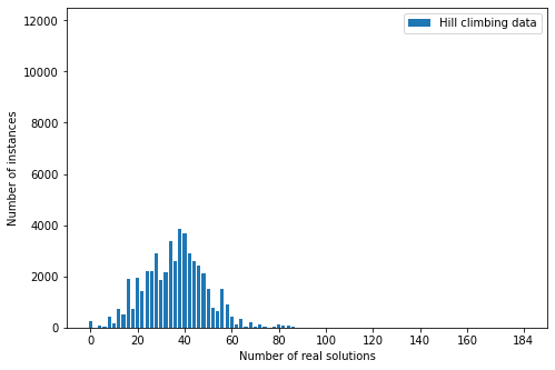
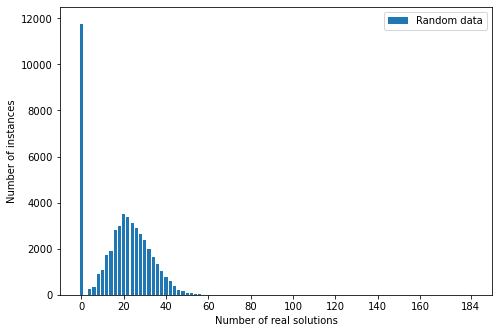
Figure 4. Two histograms showing the distribution of the number of real circles tangent to a given configuration of conics. The top histogram shows the distribution on the data $\mathcal{D}_{1}$ we generated using the hill climbing algorithm and the bottom histogram shows the distribution on random data $\mathcal{D}_{2}$.

4.2. The model

Since the number of real circles $n$ tritangent to $3$ conics is a discrete variable, our problem is a classification problem – the data space for the output variable consists of discrete points, called classes.

We found that turning our problem into a regression problem works better: Instead of having a response variable in $n\in\mathbb{N}$, we consider a statistical model

$$(p,y)\in\mathbb{R}^{18}\times\Delta_{92},$$

where $\Delta_{92}=\{y\in\mathbb{R}^{93}\mid y_{1}+\cdots+y_{93}=1,y_{i}\geq 0\}$ is the $92$-dimensional standard simplex. The underlying idea is that $y$ defines a discrete random variable where $y_{k}:=\mathrm{Prob}(y=k)$ gives the probability that for given input parameters $p\in\mathbb{R}^{18}$, the corresponding conics defined by $p$ have $2k$ real tritangent circles. For all parameters outside of the discriminant, there must be an even number of real solutions, so we have $1+\tfrac{184}{2}=93$ possibilities for the number of real zeros. The data points from the previous subsection are then encoded as the vertices of the simples; i.e., given a number of real circles $n$ we associate to it the probability distribution $y$, where $\mathrm{Prob}(y=\tfrac{1}{2}n)=1$. This process is sometimes called one hot encoding. It turns categorical data into data which can be used for regression problems.

The goal of our machine algorithm is then to learn a function

$$\phi:\mathbb{R}^{18}\to\Delta_{92}.$$

such that $\phi(p)$ is a good predictor for the number of real circles corresponding to $p$. Since $\phi(p)$ is a point in $\Delta_{92}$, we predict the number of real tritangent circles to the three conics defined by $p$ to be two times the maximum index of $\phi(p)$:

$$2\cdot\arg\max\ \{\phi(p)_{i-1}\ :\ 1\leq i\leq 93\}\in\{0,2,\ldots,184\}.$$

We model $\phi$ using a multilayer perceptron (MLP) [16]. A MLP is defined as the composition $\phi=\phi_{1}\circ\cdots\circ\phi_{m}$ of sub-functions $\phi_{0},\ldots,\phi_{m}$ called layers, where

$$\phi_{i}(x)=\sigma_{i}(W_{i}x+b_{i})$$

with matrices $W_{i}\in\mathbb{R}^{m_{i}\times m_{i+1}}$, vectors $b_{i}\in\mathbb{R}^{m_{i}}$, and a nonlinear activation function $\sigma_{i}:\mathbb{R}^{m_{i}}\to\mathbb{R}^{m_{i}}$. The matrices $W_{i}$ are called weights and the vectors $b_{i}$ are called biases. In our model we use $m=2$ layers, and do not impose any sparsity constraint on the weights. That is, we use a fully connected model. Both layers have $1,000$ neurons each, which means that $m_{1}=m_{2}=1,000$. As the nonlinear activation function we use the coordinate-wise ReLU function

$$\sigma_{i}((x_{1},\ldots,x_{m}))=(\max\{0,x_{1}\},\ldots,\max\{0,x_{m}\}),\quad i=1,2.$$

The activation function for the output is the softmax function

$$\sigma_{0}((x_{1},\ldots,x_{m}))=\frac{1}{\sum_{i=1}^{m}\exp(x_{i})}\,(\exp(x_{1}),\ldots,\exp(x_{m})).$$

We choose the categorical cross entropy loss function

$$L(y,\hat{y})=-\sum_{k=0}^{92}y_{k}\cdot\log(\hat{y}_{k}),$$

where $\hat{y}_{k}$ is the probability that there are $2k$ real solutions. In the process of training, the weights and biases are sequentially adjusted so that the loss function is minimized. To find the optimal weights and biases, we use stochastic gradient-based optimization. Backpropagation calculates the gradient of the cost function with respect to the given weights [14]. Our optimizitaion algorithm is Adam [17]. Adam requires only first order gradients and computes individual adaptive learning rates. We use a batch size of 64.

We developed the model architecture during the data exploration phase. We tried several different architectures where we varied the number of layers, the number of neurons in each layer, and the activation functions. We found that networks with more than two hidden layers or fewer neurons had slower learning progress and resulted in worse accuracy on the validation set than our proposed model.

4.3. Evaluation

We implemented the model outlined in Section 4.2 using TensorFlow [1] with data sets $\mathcal{D}_{1},\mathcal{D}_{2}$. We used an $80/20$ training-test-split and consider training our model in three ways: (1) using training data $\mathcal{D}_{1}$, (2) using training data $\mathcal{D}_{2}$ and (3) using training data $\mathcal{D}_{1}\cup\mathcal{D}_{2}$. Table 1 documents our results.

The values on the diagonal entries of Table 1 are the validation results from training. All other results are computed on the whole set. We found that the accuracy on set $\mathcal{D}_{1}$ is very low, when training only on set $\mathcal{D}_{2}$ and vice versa which is not surprising considering how different the underlying distributions of $\mathcal{D}_{1}$ and $\mathcal{D}_{2}$ are. In addition, the purely random data from data set $\mathcal{D}_{2}$ is much harder to learn than $\mathcal{D}_{1}$. The model achieves validation accuracy of $97.47\%$ on $\mathcal{D}_{1}$ against a validation accuracy of only $47.33\%$ on $\mathcal{D}_{2}$. This means that when using $\mathcal{D}_{2}$ as training data, the model is over-fitting and learning random features from the data. There are many techniques to prevent this [14] that can be explored in future work. Nevertheless, training on $\mathcal{D}_{1}$ works exceptionally well, even without any special techniques.

Training Data	Accuracy on $\mathcal{D}_{1}$	Accuracy on $\mathcal{D}_{2}$	Accuracy on $\mathcal{D}_{1}\cup\mathcal{D}_{2}$
$\mathcal{D}_{1}$	95.59%	3.68%	49.88%
$\mathcal{D}_{2}$	3.53%	47.33%	45.69%
$\mathcal{D}_{1}\cup\mathcal{D}_{2}$	90.76%	38.56%	60.20%

Table 1. The empirical results with the three different training sets

It is reasonable to expect that $\mathcal{D}_{1}$ is easier to predict than $\mathcal{D}_{2}$, because the data set $\mathcal{D}_{1}$ represents a wider range of the behavior of the parameter space. Nevertheless, as $\mathcal{D}_{1}$ only contains parameters with up to 90 real tritangent circles, it does not capture the whole picture. We believe that the good performance of $\mathcal{D}_{1}$ is implied by the structure of the real discriminant from Theorem 2.3. Learning the discriminant was approached in [3]. It would be interesting to understand to what extent the real discriminant can be learned from $\mathcal{D}_{1}$.

References

• [1] Martín Abadi, Ashish Agarwal, Paul Barham, Eugene Brevdo, Zhifeng Chen, Craig Citro, Greg S. Corrado, Andy Davis, Jeffrey Dean, Matthieu Devin, Sanjay Ghemawat, Ian Goodfellow, Andrew Harp, Geoffrey Irving, Michael Isard, Yangqing Jia, Rafal Jozefowicz, Lukasz Kaiser, Manjunath Kudlur, Josh Levenberg, Dandelion Mané, Rajat Monga, Sherry Moore, Derek Murray, Chris Olah, Mike Schuster, Jonathon Shlens, Benoit Steiner, Ilya Sutskever, Kunal Talwar, Paul Tucker, Vincent Vanhoucke, Vijay Vasudevan, Fernanda Viégas, Oriol Vinyals, Pete Warden, Martin Wattenberg, Martin Wicke, Yuan Yu, and Xiaoqiang Zheng. TensorFlow: Large-scale machine learning on heterogeneous systems, 2015. Software available from tensorflow.org.
• [2] Benjamin Alvord. Tangencies of circles and spheres. Smithsonian Contributions to Knowledge, 1855.
• [3] Edgar A. Bernal, Jonathan D. Hauenstein, Dhagash Mehta, Margaret H. Regan, and Tingting Tang. Machine learning the real discriminant locus. J. Symb. Comput., 115:409–426, 2020.
• [4] Paul Breiding, Hanieh Keneshlou, and Antonio Lerario. Quantitative Singularity Theory for Random Polynomials. International Mathematics Research Notices, 2022(8):5685–5719, 10 2020.
• [5] Paul Breiding, Kemal Rose, and Sascha Timme. Certifying zeros of polynomial systems using interval arithmetic, 2021.
• [6] Paul Breiding, Bernd Sturmfels, and Sascha Timme. 3264 conics in a second. Notices Amer. Math. Soc., 67(1):30–37, 2020.
• [7] Paul Breiding and Sascha Timme. HomotopyContinuation.jl: A package for homotopy continuation in Julia, 2018.
• [8] Taylor Brysiewicz, Claudia Fevola, and Bernd Sturmfels. Tangent quadrics in real 3-space. Matematiche (Catania), 76:355–367, 2021.
• [9] Daouda Niang Diatta and Antonio Lerario. Low-degree approximation of random polynomials. Foundations of Computational Mathematics, 22(1):77–97, 2022.
• [10] Peter Dietmaier. The Stewart-Gough Platform of General Geometry can have 40 Real Postures, pages 7–16. Springer Netherlands, Dordrecht, 1998.
• [11] David Eisenbud. Commutative Algebra, volume 150 of Graduate Texts in Mathematics. Springer-Verlag, 1995.
• [12] David Eisenbud and Joe Harris. 3264 and All That: A Second Course in Algebraic Geometry. Cambridge University Press, 2016.
• [13] Ioannis Z. Emiris and George M. Tzoumas. Algebraic study of the apollonius circle of three ellipses. In In Proc. Europ. Works. Comp. Geom, pages 147–150, 2005.
• [14] Ian Goodfellow, Yoshua Bengio, and Aaron Courville. Deep Learning. MIT Press, 2016. http://www.deeplearningbook.org.
• [15] Phillip Griffiths and Joe Harris. Principles of Algebraic Geometry. Wiley, 1994.
• [16] Kurt Hornik. Approximation capabilities of multilayer feedforward networks. Neural Networks, 4(2):251–257, 1991.
• [17] Diederik P. Kingma and Jimmy Ba. Adam: A method for stochastic optimization, 2014.
• [18] Antonio Lerario and Michele Stecconi. Maximal and typical topology of real polynomial singularities. Ann. Inst. Fourier, 2021.
• [19] Felice Ronga, Alberto Tognoli, and Thierry Vust. The number of conics tangent to five given conics: the real case. Revista Matemática de la Universidad Complutense de Madrid, 10(2):391–421, 1997.
• [20] Andrew J. Sommese and Charles W. Wampler. The Numerical Solution of Systems of Polynomials Arising in Engineering and Science. World Scientific, 2005.
• [21] Frank Sottile. Real Solutions to Equations from Geometry. University lecture series. American Mathematical Society, 2011.
• [22] Anders Thorup and Steven L. Kleiman. Intersection theory and enumerative geometry. a decade in review. section 3. volume 46, pages 332–338, 1987.