Layerwise Sparsifying Training and Sequential Learning Strategy for Neural Architecture Adaptation

Abstract

This work presents a two-stage framework for progressively developing neural architectures to adapt/ generalize well on a given training data set. In the first stage, a manifold-regularized layerwise sparsifying training approach is adopted where a new layer is added each time and trained independently by freezing parameters in the previous layers. In order to constrain the functions that should be learned by each layer, we employ a sparsity regularization term, manifold regularization term and a physics-informed term. We derive the necessary conditions for trainability of a newly added layer and analyze the role of manifold regularization. In the second stage of the Algorithm, a sequential learning process is adopted where a sequence of small networks is employed to extract information from the residual produced in stage I and thereby making robust and more accurate predictions. Numerical investigations with fully connected network on prototype regression problem, and classification problem demonstrate that the proposed approach can outperform adhoc baseline networks. Further, application to physics-informed neural network problems suggests that the method could be employed for creating interpretable hidden layers in a deep network while outperforming equivalent baseline networks.

1 Introduction

Deep neural networks (DNN) has been prominent in learning representative hierarchical features from image, video, speech, and audio inputs [1, 2, 3, 4]. Some of the problems associated with training such deep networks include [5]: i) a possible large training set is demanded to overcome the over-fitting issue; ii) architecture adaptability problem, e.g. any amendments to a pretrained DNN, requires retraining even with transfer learning; iii) GPU employment is almost mandatory for training due to massive network and data sizes. In particular, it is often unclear on the choice of depth and width of a network suitable for a specific problem. Existing neural architecture search algorithms rely on metaheuristic optimization, or combinatorial optimization, or reinforcement learning strategy to arrive at a “reasonable" architecture [6, 7]. However, this strategy involves training and evaluating many candidate architectures (possibly deep) in the process and is therefore computationally expensive. Therefore, there is a need to develop a computationally tractable procedure for adaptively training/growing a DNN by leveraging information on the input data manifold and underlying physics of the problem.

1.1 Related work

Layerwise training of neural networks is an approach that addresses the issue of the choice of depth of a neural network and the computational complexity involved with training [8]. Many attempts have been made for growing neural architecture using this approach [9, 10, 11, 5, 12, 13, 14]. Hettinger et al. [9] showed that layers can be trained one at a time, and allows for construction of deep neural networks with many sorts of learners. Belilovsky et al. [15] has further studied this approach for different convolutional neural networks. Kulkarni et al. [10] employed a kernel analysis of the trained deep networks for training each layer. The weights for each layer is obtained by solving an optimization aiming at a better representation where a subsequent layer builds its representation on the top of the features produced by a previous layer. Lengelle et al. [16] conducted a layer by layer training of MLP by optimizing an objective function for internal representations while avoiding any computation of the network’s outputs. Bengio et al. [17] proposed a greedy layer-wise unsupervised learning algorithm where upper layers of a network are supposed to represent more abstract concepts that explain the input observation $x$, whereas lower layers extract low-level features from $x$. Nguyen et al. [13] developed an analytic layer wise deep learning framework for fully connected neural networks where an inverse layer-wise learning and a forward progressive learning approach are adopted.

Alternately, researchers have also considered growing the width gradually by adding neurons for a fixed depth neural network [18, 19]. Wynne-Jones [19] considered splitting the neurons (adding neurons) based on a principal component analysis on the oscillating weight vector. Liu et al. [18] developed a simple criterion for deciding the best subset of neurons to split and a splitting gradient for optimally updating the off-springs. Chen et al. [20] showed that replacing a model with an equivalent model that is wider (has more neurons in each hidden layer) allows the equivalent model to inherent the knowledge from the existing one and can be trained to further improve the performance.

It is important to point out that existing works on layerwise adaptation rely on either supervised [9, 13] or unsupervised learning [10, 16, 17]. It is well known that each layer of the neural networks learns a particular feature and that subsequent layer builds its representation on the top of the features produced by a previous layer. Recent work by Trinh et al. [21] showed that that layerwise training quickly saturates after a certain critical layer, due to the overfitting of early layers within the networks. Therefore, it is imperative to consider a semi-supervised layer wise training strategy for efficient feature extraction at each layer and to prevent overfitting at each layer.

1.2 Our contributions

In this work, we embark on a sequential learning strategy to address the above challenges. In sequential learning, a learning task is divided into sub-tasks each of which is learnt before the next, and it is well known that the human brain learns this way [22]. A layerwise training strategy (Algorithm 1) where each layer is constrained to learn a specific map is adopted. To that end, when training each layer we incorporate a sparsity regularization for identifying the active/inactive parameters in each layer, a manifold regularization term [23], and a physics-informed term [24] in the cost function. The key in our approach is to achieve $\varepsilon-\delta$ stable neural transfer maps (hidden layers) by layerwise training. Once layerwise training saturates, we devise Algorithm 2 where a sequence of small networks are deployed to extract information from the residuals produced by Algorithm 1. Using Algorithm 2 together with Algorithm I results in robustness and accuracy. Since, the procedure emphasizes on training a small network/layer each time, it is computationally tractable for large-scale problems and is free from vanishing gradient problem. Numerical investigation on prototype regression problem, physics informed neural network problems (PINNs), and MNIST classification problem suggest that the proposed approach can outperform adhoc baseline networks.

2 Proposed methodology

The proposed architecture adaptation procedure involves two stages: a) A Layerwise Training strategy for growing neural networks along the depth; b) Sequential learning strategy where one uses a sequence of small networks for robust and accurate predictions.

2.1 Layerwise training strategy (Algorithm 1)

One of the key aspects in the layerwise training strategy is the use of Residual Neural Network [25, 26] which, as we will show, improves the training loss accuracy when adding new layers. Consider a regression/classification problem of $O$ outputs and $S$ input training features. Given inputs $\mathbf{x}_{m}\in\mathbb{R}^{S}$ for $m\in\{1,2,...M\}$ organized row-wise into a matrix $\mathbf{X}\in\mathbb{R}^{M\times S}$, we denote the corresponding network outputs as $\mathbf{y}_{m}\in\mathbb{R}^{O}$ which can also be organized row-wise into a matrix $\mathbf{Y}\in\mathbb{R}^{M\times O}$. The corresponding true labels are denoted as $\mathbf{c}_{m}\in\mathbb{R}^{O}$ and in stacked row-wise as $\mathbf{C}\in\mathbb{R}^{M\times O}$.

We begin by detailing a ResNet propagation before introducing the layerwise training strategy. For the present approach, we consider an affine mapping that upsamples/downsamples our inputs $\mathbf{X}$. We denote $\mathbf{Y}^{(1)}=\mathbf{X}\mathbf{U}+{\bf u}$, where $\mathbf{U}$ represents the weight matrix for this layer. $\mathbf{Y}^{(1)}$ is then propagated forward through the ResNet as:

$$\mathbf{Y}^{(1)}=\mathbf{X}\mathbf{U}+{\bf u},$$ (1)

$$\mathbf{Y}^{(l+1)}=\mathbf{Y}^{(l)}+h^{(l+1)}(\mathbf{Y}^{(l)}\mathbf{W}^{(l+1)}+{\bf b}^{(l+1)}),\textrm{ for }l=1,\dots,L-1,$$

$$\mathbf{Y}^{(L+1)}=h_{pred}(\mathbf{Y}^{(L)}\mathbf{W}_{pred}+\mathbf{b}_{pred}),$$

where $h^{(l+1)},\mathbf{W}^{(l+1)},{\bf b}^{(l+1)}$ are the activation function, weight matrix, and bias vector of layer $(l+1)$, while $h_{pred},W_{pred},\mathbf{b}_{pred}$ are the activation function, weight matrix, and bias vector of the output layer.

For our layerwise training strategy, we incorporate there different regularization strategies, namely, (a) Sparsity regularization; (b) Manifold regularization; and (c) Physics-informed regularization:

• Sparsity Regularization: Sparse regularization allows for learning only those weights/biases which are essential to the task at hand, while other weights/biases are set to zero [27, 28]. In this case, we use the $L_{1}$ sparsifying regularization defined as:

  $$L_{s}(\vec{\theta})=\left\|\vec{\theta}\right\|_{1},$$ (2)

  where $\vec{\theta}$ represents the vector of trainable network parameters.

• Manifold Regularization (Data-informed regularization):

  Manifold regularization exploits the geometry of marginal distribution where we assume that the input data is not drawn uniformly from input space ${\mathcal{X}}$ but lies on a manifold ${\mathcal{M}}\subset{\mathcal{X}}$ [23]. Let $\mu$ be a probability measure with support ${\mathcal{M}}$. Then, the formulation of manifold regularization term is as follows [29]:

  $$L_{m}^{l}=\frac{M^{2}}{2}\int_{{\mathcal{M}}}\left\|\nabla_{{\mathcal{M}}}\ y^{l}(x)\right\|^{2}\ d\mu(x)\xrightarrow[\text{}]{\text{approximated}}\frac{1}{2}\sum_{i,j}\beta_{ij}||\mathbf{Y}^{l}_{i}(\vec{\theta}^{l})-\mathbf{Y}^{l}_{j}(\vec{\theta}^{l})||^{2},$$ (3)

  where $y^{l}(x)$ is the output of the $l^{th}$ hidden layer for an input $x$. Let $\mathbf{Y}^{l}$ represents output for the $l^{th}$ layer and the subscript $i$ denotes the $i^{th}$ row vector (i.e corresponding to $i^{th}$ training sample) Here, $\beta_{ij}$ is the similarity matrix, and ${\vec{\theta}}^{l}$ represents the trainable network parameters upto layer $l$. Thus, Equation (3) assumes that the gradient of the learnt function $y^{l}(x)$ should be small whenever the probability of drawing a sample is large. For the present approach, similarity matrix is chosen as:

  $$\beta_{ij}=\begin{cases}1&\text{for }\mathbf{c}_{i}=\mathbf{c}_{j},\\ 0&\text{otherwise }\end{cases}$$ (4)

  where, $\mathbf{c}_{i}$ denotes the label corresponding to training point $\mathbf{x}_{i}$. In case of regression problem, one may use $\varepsilon$ nearest neighbours or K-means clustering for computing $\beta_{ij}$. Regularization of this form ensures that each layer learns meaningful representations for similar training data point.

• Physics-informed regularization: In addition to the training data, if one is also provided with information on the underlying physics of the problem, then each hidden layer can be trained to respect the governing laws [24] as well. To that end, given a forward operator of algebraic/ differential equation type:

  $${\mathcal{G}}(\hat{\mathbf{x}},\ \hat{\mathbf{y}})=\bf{0},\ \ \ \ \hat{\mathbf{x}}\in{\mathbb{R}}^{S},\ \ \hat{\mathbf{y}}\in{\mathbb{R}}^{O},$$ (5)

  physics-informed regularization term can be defined as:

  $$L_{p}(\vec{\theta})=f\left[{\mathcal{G}}(\hat{\mathbf{x}}_{1},\ {\mathcal{N}}(\hat{\mathbf{x}}_{1})),\ {\mathcal{G}}(\hat{\mathbf{x}}_{2},\ {\mathcal{N}}(\hat{\mathbf{x}}_{2})),\dots\ {\mathcal{G}}(\hat{\mathbf{x}}_{r},\ {\mathcal{N}}(\hat{\mathbf{x}}_{r}))\right]\in{\mathbb{R}},$$ (6)

  where, ${\mathcal{N}}$ is the ResNet in Eq. 1 with parameters $\vec{\theta}$. $\{\hat{\mathbf{x}}_{1}\dots\hat{\mathbf{x}}_{r}\}$ is the set of collocation points, and $f$ is the loss defined such that $f\geq 0$.

Putting all the regularizations together, our layerwise training process is shown in Algorithm 1.

Algorithm 1 Greedy Layer wise training Algorithm

Input: Training data $\mathbf{X}$, labels $\mathbf{C}$, validation data $\mathbf{X}_{1}$, validation labels $\mathbf{C}_{1}$, loss tolerance $\varepsilon_{\eta}$ for addition of layers, node tolerance $\rho$ for thresholding of nodes, regularization parameter ($\alpha$, $\delta$, $\gamma$), learning rate $l_{r}$, the number of epochs $E_{e}$, learning rate decay $d_{l}$, the number of neurons in each hidden layer $o$.
      Initialize: Allocate $\bf{U},{\bf u},\bf{W}^{(2)},{\bf b}^{(2)},\bf{W}_{\mathrm{pred}},{\bf b}_{\mathrm{pred}}$

1:set $L=2$

2:Minimize the cost function using Adam optimizer with parameters ($l_{r}$, $d_{l}$) and $E$ epochs:

$$\min_{\mathbf{U},{\bf u},\bf{W}^{(2)},{\bf b}^{(2)},W_{\mathrm{pred}},{\bf b}_{\mathrm{pred}}} \frac{1}{S}E(\mathbf{C},h_{\mathrm{pred}}(\mathbf{Y}^{(2)}\mathbf{W}_{\mathrm{pred}}+{\bf b}_{\mathrm{pred}}))+\alpha\times L_{s}(\mathbf{U},{\bf u},\mathbf{W}^{(2)},{\bf b}^{(2)})$$ (7)

$$+\ \delta \times L_{p}(\mathbf{U},{\bf u},\mathbf{W}^{(2)},\mathbf{W}_{\mathrm{pred}},{\bf b}^{(2)},{\bf b}_{\mathrm{pred}})+\gamma\times L_{m}^{2}(\mathbf{U},{\bf u},\bf{W}^{(2)},{\bf b}^{(2)}),$$

$$\mathrm{subject}\>\mathrm{to} \mathbf{Y}^{(2)}=\mathbf{Y}^{(1)}+h^{(2)}(\mathbf{Y}^{(1)}\mathbf{W}^{(2)}+{\bf b}^{(2)}),$$

$$\mathbf{Y}^{(1)}=\mathbf{X}\mathbf{U}+{\bf u}.$$

3:Define: $\eta^{L}=\Big{(}\frac{1}{S}E(\mathbf{C},h_{\mathrm{pred}}(\mathbf{Y}^{(L)}\mathbf{W}_{\mathrm{pred}}+{\bf b}_{\mathrm{pred}}))\Big{)},\ \ given\ \eta^{1}\approx 0$

4:while  $\frac{\eta^{L-1}-\eta^{L}}{\eta^{L-1}}>\varepsilon_{\eta}$ do

5:     $L=L+1$

6:     Extend the neural network by one layer with weights $\mathbf{W}^{(L)}$ and ${\bf b}^{(L)}$ initialized as zero.

7:     Initialize $\mathbf{W}_{\mathrm{pred}}$ and ${\bf b}_{\mathrm{pred}}$ with values inherited from the previously trained network.

8:     Freeze the weights $\mathbf{U},{\bf u},\{\mathbf{W}^{(l)}\}_{l=1}^{L-1},\{{\bf b}^{(l)}\}_{l=1}^{L-1}$ so that they are not trainable.

9:     Minimize the below objective using Adam optimizer with parameters ($l_{r}$, $d_{l}$) and $E$ epochs:

$$\min_{\mathbf{W}^{(L)},\bf{b}^{(L)}\,\mathbf{W}_{\mathrm{pred}},{\bf b}_{\mathrm{pred}}} \frac{1}{S}E(\mathbf{C},h_{\mathrm{pred}}(\mathbf{Y}^{(L)}\mathbf{W}_{\mathrm{pred}}+{\bf b}_{\mathrm{pred}}))+\alpha^{L}\times L_{s}(\mathbf{W}^{(L)},{\bf b}^{(L)})$$ (8)

$$+\ \delta^{L} \times L_{p}(\mathbf{W}^{(L)},\mathbf{W}_{\mathrm{pred}},{\bf b}^{(L)},{\bf b}_{\mathrm{pred}})+\gamma^{L}\times L_{m}^{L}(\bf{W}^{(L)},{\bf b}^{(L)}),$$

$$\mathrm{subject}\>\mathrm{to} \mathbf{Y}^{(l+1)}=\mathbf{Y}^{(l)}+h^{(l+1)}(\mathbf{Y}^{(l)}\mathbf{W}^{(l+1)}+{\bf b}^{(l+1)}),\textrm{ for }l=1,\dots,L-1$$

$$\mathbf{Y}^{(1)}=\mathbf{X}\mathbf{U}+{\bf u}.$$

10:     Threshold weights and biases: if $\Big{|}w_{ij}^{(L)}\Big{|},\ \Big{|}b_{j}^{(L)}\Big{|}<\rho$ then set $w_{ij}^{(L)},\ b_{j}^{(L)}=0$.

11:end while

2.2 Sequential learning strategy (Algorithm 2)

We note that even though Algorithm 1 proposed in this work prevents overfitting in early layers, training saturates after certain critical layer (Remark 1). To overcome this issue, we incorporate a sequential learning strategy for accurate prediction. The idea of sequential learning is to train a sequence of small neural networks to extract information from the residual resulting from Algorithm 1 (Layerwise training) thereby further improving the generalization performance. The procedure is shown in Algorithm 2. Note that in each step of Algorithm 1 and Algorithm 2, we train either an individual layer or a small network (small number of parameters) each time and is therefore parameter efficient.

Algorithm 2 Sequential learning

Input: Training data $\mathbf{X}$, labels $\mathbf{C}$, validation data $\mathbf{X}_{1}$, validation labels $\mathbf{C}_{1}$, trained network ${\mathcal{N}}_{1}$ from Algorithm 1 with $L+1$ layers, loss tolerance $\varepsilon_{e}$, expected decrease in validation loss by Network ${\mathcal{N}}_{i}$= $\eta_{i}$.
      Initialize: Maximum number of networks: $N_{n}$, initialize each network: ${\mathcal{N}}_{i}$ with $\leq 2$ hidden layers.

1:set $i=1$, $e^{0}\approx 0$

2:while $i\leq N_{n}$ and $\frac{e^{i-1}-e^{i}}{e^{i-1}}>\varepsilon_{e}$ do

3:     Load network ${\mathcal{N}}_{i}$

4:     $\mathbf{C}=\mathbf{C}-{\mathcal{N}}_{i}(\mathbf{X})$

5:     Train network ${\mathcal{N}}_{i+1}$ with data $\mathbf{X}$ and labels $\mathbf{C}$. Train for $E_{i+1}$ epochs and early stopped if val. loss$<\eta_{i+1}$

6:     Save the new network ${\mathcal{N}}_{i+1}$ and the corresponding training loss $e^{i+1}$

7:     $i=i+1$

8:end while

9:Compute the net output as: $\mathbf{Y}={\mathcal{N}}_{1}(\mathbf{X})+{\mathcal{N}}_{2}(\mathbf{X})+\dots\mathcal{N}_{r}(\mathbf{X})$,      where $r=N_{n}+1$

3 Mathematical description of Algorithm I and Algorithm II

3.1 Layerwise training Algorithm 1

In Algorithm 1, the input features are transformed through the layers to create a new learning problem each time. To that end, let us define the following:

Definition 1

Neural transfer map and layerwise training data set

Define the neural transfer map ${\mathcal{N}}_{1}^{i}:{\mathcal{X}}^{(i-1)}\rightarrow{\mathcal{X}}^{i}$ for training the $(i+1)^{th}$ hidden layer as:

$${\mathcal{N}}_{1}^{i}\left(\mathbf{X}^{(i-1)}\right)=\mathbbm{1}_{A}(i)\ \mathbf{X}^{(i-1)}{\mathcal{I}}+h^{(i)}\left(\mathbf{X}^{(i-1)}\hat{\mathbf{W}}^{(i)}+{\bf\hat{b}}^{(i)}\right),$$ (9)

where, $A=\{2,\ 3,\ 4,\ \dots\}\subset\mathbb{N}$, $\mathbbm{1}_{A}(i)$ is the indicator function, ${\mathcal{I}}$ is the identity matrix for addition compatibility, and $h^{i}$ represents the ‘elu’ activation for $i>1$ but an identity map otherwise. $\hat{\mathbf{W}}^{(i)}$ and ${\bf\hat{b}}^{(i)}$ are fixed weights and biases. The new data set ${\mathcal{K}}^{i+1}_{I}$ for training the $(i+1)^{th}$ hidden layer with parameters ${\mathbf{W}}^{(i+1)}$ and ${\bf{b}}^{(i+1)}$ is then defined as:

$${\mathcal{K}}^{i+1}_{I}=\Big{\{}{\mathcal{N}}_{1}^{i}\left(\mathbf{X}^{(i-1)}\right),\ \mathbf{C}\Big{\}}=\Big{\{}\mathbf{Y}^{(i)},\ \mathbf{C}\Big{\}}.$$ (10)

A key aspect of the algorithm is to create transfer maps ${\mathcal{N}}_{1}^{i}$ that allows for effective information transfer through the network. In fact, each layer of a deep neural network can be regarded as an “information filter" [16]. In this work, we focus on creating transfer maps ${\mathcal{N}}_{1}^{i}$ that are $\varepsilon-\delta$ stable for a given input $x$ through the use of manifold regularization [29]. A schematic of Algorithm 1 is given in Figure 1.

Definition 2

Layerwise training promoting property (LTP)

A non-linear activation function $h(\cdot)$ holds the layerwise training promoting property (LTP) if the following conditions are satisfied:

• $h(0)=0$,

• $h^{\prime}(0)\neq 0$.

It is easy to see that activation functions such as ‘ELU’ and ‘Tanh’ satisfies the LTP property, whereas ‘Sigmoid’ and ‘ReLU’ do not satisfy the LTP property. However, any activation function can be forced to satisfy the LTP property through an affine transformation.

In this work, the activation functions $h^{l}$ for $l=\{2,3,...L\}$ in Algorithm 1 is selected to be the exponential linear unit (ELU) ([30]).

Proposition 1 (Necessary condition for trainability of newly added layer.)

Consider training the $(i+1)^{th}$ hidden layer with the parameters $\mathbf{W}^{(i+1)}$ and ${\bf b}^{(i+1)}$ initialized as zero. With this initialization, the newly added layer preserves the previous layer’s output and is trainable only if $\gamma^{i+1}\neq\gamma^{i}$ or $\delta^{i+1}\neq\delta^{i}$ and the activation $h^{(i+1)}$ satisfies the LTP property. Furthermore, let $E^{i*}$ denote the final value of the data loss function after training the $i^{th}$ layer. Then, the loss at $n^{th}$ iteration in training the $(i+1)^{th}$ layer, $E^{i+1}_{n}<E^{i*}$ if $\gamma^{i+1}<\gamma^{i}$ and $\delta^{i+1}<\delta^{i}$ and the activation $h^{(i+1)}$ satisfies the LTP property.

Corollary 1 (Monotonically decreasing loss with layer addition and training saturation)

The loss is monotonically decreasing as number of layers increases, i.e $E^{i*}<E^{(i-1)*}\ \ \forall i$, and thus $E^{i*}\rightarrow\rho$, where $\rho\geq 0$ as $i\rightarrow\infty$.

Remark 1 (Implicit regularization imposed by layerwise training saturation)

Note that manifold regularization is decreased with layerwise addition i.e, $\gamma^{i+1}<\gamma^{i}$. Thus, while initial layers create meaningful data representation, the later layers focus on the actual classification/regression task in hand. Furthermore, the fact that $E^{i*}\rightarrow\rho$ (training saturation) for sufficiently large $i$ acts as an implicit regularizer preventing overfitting in later layers.

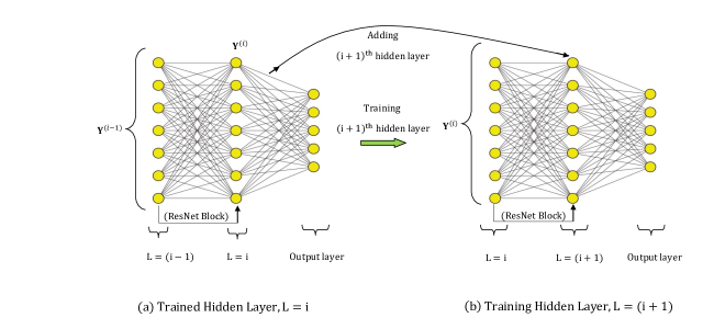
Figure 1: Schematic of Algorithm 1.

Proposition 2 ($\varepsilon-\delta$ stable transfer maps)

Assume that the true underlying map $f^{*}(x)$ is smooth on the data manifold ${\mathcal{M}}\subset{\mathcal{X}}$ and relevant subset of the data comes from ${\mathcal{M}}_{j}\subset{\mathcal{M}}$ such that ${\mathcal{M}}=\bigsqcup\limits_{j=1}^{K}{\mathcal{M}}_{j}$. Now, consider training the $(i+1)^{th}$ hidden layer. Let us denote ${\mathcal{K}}^{i+1}_{I}\left(\gamma^{1},\ \gamma^{2},\ \gamma^{3},\dots\gamma^{i}\right)$ as the generated data set. Let the trained neural transfer map for the $(i+1)^{th}$ hidden layer be denoted as ${\mathcal{N}}^{i+1}_{1}\left({\mathcal{K}}^{i+1}_{I},\ \gamma^{i+1}\right)$. Then, at any given input $x\in{\mathcal{M}}^{i}\subset{\mathcal{X}}^{i}$, $\forall\varepsilon$, $\exists\ \delta=\delta(\gamma^{i+1},\ x,\ \varepsilon)>0$ such that:

$$\left\|{\mathcal{N}}^{i+1}_{1}\left(x,\ \gamma^{i+1}\right)-{\mathcal{N}}^{i+1}_{1}\left(x^{\prime},\ \gamma^{i+1}\right)\right\|_{2}\leq\delta,\ \ \ \ \ \ \ \ \ \forall x^{\prime}\in B_{\varepsilon}(x),$$ (11)

where, ${\mathcal{X}}^{i}$ represents the entire input space for the transfer map ${\mathcal{N}}_{1}^{i+1}$. $B_{\varepsilon}(x)$ denotes the open ball centered at $x$ with radius $\varepsilon$ in the metric space $({\mathcal{M}}_{j}^{i},\ d)$ for some ${\mathcal{M}}_{j}^{i}\subset{\mathcal{M}}^{i}\subset{\mathcal{X}}^{i}$. Thus, $\delta$ could be made arbitrarily small (hence promoting stability) by varying $\gamma^{i+1}$.

Remark 2 (Role of sparsity regularization)

By initializing the weights of each neural transfer maps ${\mathcal{N}}_{1}^{i}$ as zero, sparsity regularization encourages learning only the most relevant parameters. $L_{1}$ regularization further contributes to the $\varepsilon-\delta$ stability by bounding the Lipschitz constant of ${\mathcal{N}}_{1}^{i}$ [31].

3.2 Sequential learning Algorithm 2

Recall that $\varepsilon-\delta$ stable neural transfer maps does not guarantee that the network classifies/ regress correctly. To overcome this issue, we incorporate a sequential learning strategy in Algorithm 2 for accurate prediction. The idea of sequential learning is to train a sequence of small neural networks to learn the residual in the network obtained from Algorithm 1.

Algorithm 2 creates new training problem for each network ${\mathcal{N}}_{i+1}$ by generating data sets of the form:

$${\mathcal{K}}^{i+1}_{II}=\Big{\{}\mathbf{Y}^{(0)},\ \mathbf{C}^{(i)}\Big{\}},\hskip 28.45274pt\mathbf{C}^{(i)}=\mathbf{C}^{(i-1)}-{\mathcal{N}}_{i}(\mathbf{Y}^{(0)}),\hskip 28.45274pt\ i=1,\ 2,\dots,\\$$ (12)

where, $\mathbf{C}^{(0)}=\mathbf{C}$ and ${\mathcal{N}}_{1}$ is the neural network produced by Algorithm 1.

Definition 3 (Robustness)

The function $f(x)={\mathcal{N}}_{1}(x)+{\mathcal{N}}_{2}(x)+\dots\mathcal{N}_{r}(x)$ is called $\varepsilon-\delta$ robust at an input $x$ if each network ${\mathcal{N}}_{i}$ is $\varepsilon-\delta$ stable and $f(x)=c$, where $c$ is the correct label for $x$.

Note that we enforce ${\mathcal{N}}_{1}$ (final network from Algorithm 1) to be $\varepsilon-\delta$ stable through the use of manifold regularization. The proposition 3 below shows a feasible way of controlling $\varepsilon-\delta$ stability in Algorithm 2.

Proposition 3 ($\varepsilon-\delta$ stable networks from Algorithm 2)

Consider the neural network ${\mathcal{N}}_{i}$ with input $x\in{\mathcal{M}}\subset{\mathcal{X}}$ and assume that ${\mathcal{N}}_{i}$ are locally Lipschitz continuous. Further, assume that relevant subset of the data comes from ${\mathcal{M}}_{j}\subset{\mathcal{M}}$ such that ${\mathcal{M}}=\bigsqcup\limits_{j=1}^{K}{\mathcal{M}}_{j}$. Then with $x\in{\mathcal{M}}_{j}$, $\forall\varepsilon$, $\exists\ \delta={\mathcal{L}}(x,\ {\mathcal{M}}_{j})\times\varepsilon>0$ such that:

$$\left\|{\mathcal{N}}_{i}\left(x\right)-{\mathcal{N}}_{i}\left(x^{\prime}\right)\right\|_{2}\leq\delta,\ \ \ \ \ \ \ \ \ \forall x^{\prime}\in B_{\varepsilon}(x),$$ (13)

where ${\mathcal{L}}(.,\ {\mathcal{M}}_{j})$ represents the local Lipschitz constant of ${\mathcal{N}}_{i}$ taken with respect to ${\mathcal{M}}_{j}$ and $B_{\varepsilon}(x)$ denotes the open ball centered at $x$ with radius $\varepsilon$ in the metric space $({\mathcal{M}}_{j},\ d)$. That is, network ${\mathcal{N}}_{i}$ is $\varepsilon-\delta$ stable at input $x$ with $\delta={\mathcal{L}}(x,\ {\mathcal{M}}_{j})\times\varepsilon$.

Proof:

The proof follows directly from the definition of Lipschitz continuity and stability defined in proposition 2.

Remark 3 (Achieving $\varepsilon-\delta$ stable networks from Algorithm 2)

Proposition 3 shows that $\varepsilon-\delta$ stability in Algorithm 2 can be controlled by bounding ${\mathcal{L}}(x,\ {\mathcal{M}}_{j})$ for each $j$. Further, since ${\mathcal{M}}_{j}\subset{\mathcal{M}}\subset{\mathcal{X}}$, it is sufficient to bound ${\mathcal{L}}(x,\ {\mathcal{X}})$. A classical way to do this is to choose networks with few parameters or training with a small number of epochs which restricts the Lipschitz constant and impacts the generalization gap [31].

Remark 4 (Achieving robustness)

In addition, we attempt to achieve robustness by using Algorithm 2 to the learn the sequence of residuals given by Eq. 12. Note that for an input $x$ in the training data set, $\varepsilon=|f(x)-c|$ gets smaller and smaller with the addition of each network.

4 Numerical Experiments

The experimental settings for all the problems are described in Appendix D.

4.1 Regression task: Boston house price prediction problem

This regression problem aims to predict the housing prices in Boston and is a common prototype problem for testing ML regression algorithms [11, 32, 33]. The training/testing data set is generated following a $70-30$ split rule. For this problem, the manifold regularization is computed by employing the K-means clustering algorithm on the input features [34] and the number of clusters $K$ is chosen as $5$. In addition, we also enforce adaptive regularization for $(\alpha,\gamma)$ as given in Appendix E. The input setting for Algorithm 1 is given in Appendix J.

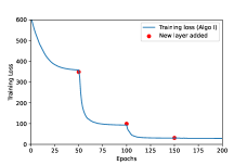
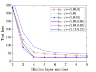
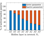
Figure 2: Left to right: Layerwise training curve on Boston house price prediction problem by Algorithm 1; Importance of sparsity ($\alpha$) and manifold regularization ($\gamma$) in Algorithm 1; Active and inactive parameters in each hidden layer.

The layerwise training curve is shown in the Figure 2. As can be observed a significant decrease in loss (ridge) is achieved when adding a new layer. This shows that, subsequent layers are able to learn on top of the representations of previous layers. The percentage of active and inactive parameters (consequence of sparsity regularization) in each layer is shown in Figure 2. We see that the weights in the initial layers matter more in a deep neural network [35]. We also note that Algorithm 1 is only capable of reducing the testing loss to $\rho=24.2$ and training saturates as predicted in corollary 1.

Further, ablation study for hyperparameters $(\alpha,\gamma)$ is conducted. From Figure 2, it is evident that in the absence of manifold regularization (i.e $\gamma=0$), stability is not explicitly enforced on each subset of the data manifold and consequently the testing loss is considerably higher in this case. Note that, the training loss is almost the same for all the cases.

In order to further decrease the testing loss, we resort to Algorithm 2. The inputs for Algorithm 2 are given in Appendix J. The adaptation results and performance comparison with other methods (the baseline and the approach from [9]) are summarized in Figure 3. Baseline network represents a fully-connected deep neural network with the same depth and width as that of the layerwise training Algorithm 1. From Figure 3, it is clear that our proposed approach outperformed the baseline network by a good margin. The number of trained parameters in each step of Algorithm 2 and from other methods is provided as a Table in Figure 3. As can be seen, the proposed two-stage approach is the most accurate (by a large margin) with the least number of network parameters. Note that using Algorithm 2 on top of the baseline network did not provide much improvement since baseline network lacks the $\varepsilon-\delta$ stability (necessary condition) required for robustness.

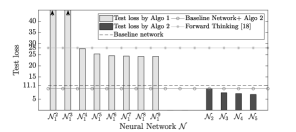
Method Test Params. trained Total loss simultaneously params. Proposed 7.11 $11,601$ 48, 474 Baseline 11.2 $82,301$ 82, 301 Regularized- 10.3 $82,301$ 82, 301 Baseline Forward- Thinking [9] 28.0 $11,601$ 82, 301

Figure 3: Boston house price prediction problem. Comparison between the proposed approach and other methods. As can be seen, the proposed two-stage approach is the most accurate (by a large margin) with the least number of network parameters.

4.2 Physics informed adaptive neural network (PIANN)

Consider the partial differential equation of the form:

$${\mathcal{G}}(\mathbf{x},\mathbf{y},a) =0,\ \ in\ \ {\mathcal{D}},$$ (14)

$$\mathbf{y} =g\ \ \ in\ \ \partial{\mathcal{D}},$$

where, $a\in{\mathcal{A}}$ is the PDE coefficient, ${\mathcal{A}}$ is the parameter space, $y\in{\mathcal{B}}$ is the unknown solution, ${\mathcal{B}}$ is the solution space and the operator ${\mathcal{G}}:{\mathcal{B}}\times{\mathcal{A}}\rightarrow{\mathcal{F}}$ is in general a non-linear partial differential operator. The objective is to find the unknown solution. For the present study, we adopt a discrete PINNs (dPINNs) approach to alleviate the problems associated with traditional PINNs [36] (see Appendix F) and adopt a continuation approach to progressively learn the solution. By choosing $\delta^{i+1}>\delta^{i}$ ($\delta$ is the weight on the physics loss), we ensure that a newly added layer is trainable in this approach (Proposition 1). Also, since $|\delta^{i+1}-\delta^{i}|\neq 0$ for any $i$, training saturation problem does not exist in this case (Corollary 1) and Algorithm 2 is not essential.

4.2.1 Learning solutions of Poisson equation

For demonstration, we consider solving the Poisson equation where the operator ${\mathcal{G}}(\mathbf{x},\mathbf{y},a)$ in Eq. 14 is given as: ${\mathcal{G}}(\mathbf{x},\mathbf{y},a)=-\nabla.(a(x_{1},\ x_{2})\nabla y)-f(x_{1},x_{2})\ \ \ in\ \ \Omega\subset{\mathbb{R}}^{2}$ with $y=0\ \ in\ \partial{\mathcal{D}}$.

We consider two different domains: case a): $\Omega=(0,1)\times(0,1)$ and case b): $\Omega=(0,1)\times(0,1)-(0.5,1)\times\{0.5\}$ [37]. $a=1$ and $f=200$. The training details are given in Appendix F. The evolution of PDE solution $y(\mathbf{x})$ as more layers are added for Case (b) is shown in Figure 4: with $L=6$ layers the solution looks identical to the finite element solution. Note that learning the solution progressively by our proposed approach outperformed a baseline trained under similar settings as seen from Figure 5. The result for case (a) and other details are given in Appendix F. It can be seen, layerwise training procedure by Hettinger et al. [9] did not perform well since the output is not preserved while adding new layers. The summary of results and parameter efficiency is provided in Appendix F. Note that the present approach leads to interpretable hidden layers in a deep neural network which could be used for devising efficient model correction strategies when new data is available (Appendix F.2.1).

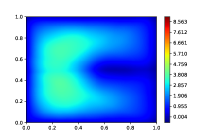
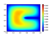
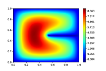
Figure 4: Adaptively learning the Poisson’s equation (Case b: Slit in domain). Left to right: solutions after $L=2$ layers, $L=3$ layers, and $L=5$ layers.

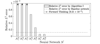
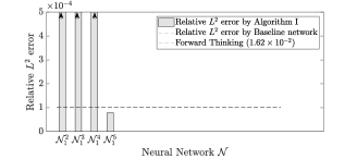
Figure 5: PIANN problem. Comparison of the proposed approach and others. Poisson problem with symmetric boundary condition (left figure), and with slit in domain (right figure).

4.3 Image classification problem: MNIST Data Set

Finally, we consider the MNIST handwritten digit classification problem using fully connected neural network. The training-validation data set is generated following a 80-20 split rule. The training curve and parameter efficiency is provided in Appendix I. Other details on input parameters can be found in Appendix J. Figure 6 shows that the proposed methodology outperforms the baseline network and other methods by noticeable margins.

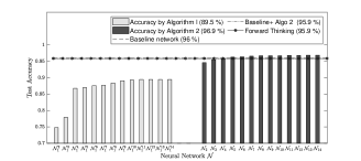
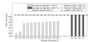
Figure 6: MNIST classification problem. Left figure is with 20 neurons in each hidden layer: our approach provides the best results with 96.9% testing accuracy. Right figure is with 500 neurons in each hidden layer: our approach provides the best results with 98.7% testing accuracy.

5 Concluding remarks

In this paper, we presented a two-stage procedure for adaptively growing neural networks to generalize well on a given data-set. The first stage (Algorithm 1 ) is designed to focus on growing a neural network along the depth and trimming the width. The second stage (Algorithm 2) is constructed to achieve accuracy. Results on prototype machine learning tasks suggest that the proposed approach can outperform an adhoc baseline and other networks. We have also additionally demonstrated the approach on problems such as: i) Adaptive learning for inverse problems (Appendix H) ii) Physics reinforced adaptive neural network (Appendix G). One bottleneck with the approach is the computational complexity of $\mathcal{O}(n^{2})$ associated with computing the manifold regularization term, where $n$ is the number of training data samples. However, this can be addressed using sub-sampling approaches [38], thereby substantially improving computational efficiency.

Appendix A Proof of proposition 1

Proof:

The ResNet forward propagation for the newly added layer with weights and biases initialized as $zero$ gives:

$$\mathbf{Y}^{(i+1)}=\mathbf{Y}^{(i)}+h^{(i+1)}(\mathbf{Y}^{(i)}{\bf{0}}+{\bf{0}}).$$ (15)

If the activation $h^{(l+1)}$ satisfies the LTP property, then we have $h^{(l+1)}(\mathbf{Y}^{(i)}{\bf{0}}+{\bf{0}})={\bf{0}}$. Therefore, $\mathbf{Y}^{(i+1)}=\mathbf{Y}^{(i)}$ on adding the new layer at the beginning of training process. Therefore, the output is given as:

$$\mathbf{Y}^{(i+2)}=h_{\mathrm{pred}}(\mathbf{Y}^{(i+1)}\mathbf{W}_{\mathrm{pred}}+{\bf b}_{\mathrm{pred}})=h_{\mathrm{pred}}(\mathbf{Y}^{(i)}\mathbf{W}_{\mathrm{pred}}+{\bf b}_{\mathrm{pred}}),$$ (16)

showing that the output is preserved and we have $E^{i+1}_{0}=E^{i*}$ at the beginning of training process. Further, using Eq. 15, the gradient for the newly added layer at the beginning of training process can be written as (see Appendix C):

$$\frac{\partial\mathcal{L}}{\partial\mathbf{W}^{(i+1)}}=-\left[\left(\mathbf{W}_{\mathrm{pred}}^{T}\left[h_{\mathrm{pred}}^{\prime}(\mathbf{Y}^{(i)}_{j}\mathbf{W}_{\mathrm{pred}}+{\bf b}_{\mathrm{pred}})\circ{(\mbox{\boldmath$\lambda$}^{2})^{i+1}}\right]-\frac{\partial L_{m}^{i+1}}{\partial\mathbf{Y}^{(i)}_{j}}\right)\circ\left({h^{(i+1)}}^{\prime}({\bf{0}})\right)\right]{\mathbf{Y}^{(i)}_{j}}^{T},$$ (17)

$$\frac{\partial\mathcal{L}}{\partial\mathbf{b}^{i+1}}=-\left[\left(\mathbf{W}_{\mathrm{pred}}^{T}\left[h_{\mathrm{pred}}^{\prime}(\mathbf{Y}^{(i)}_{j}\mathbf{W}_{\mathrm{pred}}+{\bf b}_{\mathrm{pred}})\circ{(\mbox{\boldmath$\lambda$}^{2})^{i+1}}\right]-\frac{\partial L_{m}^{i+1}}{\partial\mathbf{Y}^{(i)}_{j}}\right)\circ\left({h^{(i+1)}}^{\prime}({\bf{0}})\right)\right],$$ (18)

where $({\mbox{\boldmath$\lambda$}^{2}})^{i+1}=\left(\mathbf{C}_{j}-\mathbf{Y}^{(i+2)}_{j}\right)-\frac{\partial L_{p}^{i+1}}{\partial\mathbf{Y}^{(i+2)}_{j}}$. Note that the sparsity gradient is zero initially. Therefore, it is clear that ${h^{(i+1)}}^{\prime}({\bf{0}})\neq 0$ (LTP property) is a necessary condition for trainability of the newly added layer. Further, if the previous layer, i.e $i^{th}$ layer is trained to the local minima, then one has the following conditions (see Appendix C):

$$\left(\mathbf{W}_{\mathrm{pred}}^{T*}\left[h_{\mathrm{pred}}^{\prime}(\mathbf{Y}^{(i)}_{j}\mathbf{W}_{\mathrm{pred}}^{*}+{\bf b}_{\mathrm{pred}}^{*})\circ{(\mbox{\boldmath$\lambda$}^{2})^{i}}\right]-\frac{\partial L_{m}^{i}}{\partial\mathbf{Y}^{(i)}_{j}}\right)\circ\left({h^{(i)}}^{\prime}(\mathbf{Y}^{(i-1)}_{j}\mathbf{W}^{(i)*}+\mathbf{b}^{i*})\right)=0,$$ (19)

where, we have ignored the sparsity gradient w.r.t each parameter which is very small when choosing small $\alpha^{i}$ for our practical settings. Since, we are interested in the case where ${h^{(i)}}^{\prime}(\mathbf{Y}^{(i-1)}_{j}\mathbf{W}^{(i)*}+\mathbf{b}^{i*})\neq 0$, the above condition leads to the following:

$$\frac{\partial L_{m}^{i}}{\partial\mathbf{Y}^{(i)}_{j}}=\mathbf{W}_{\mathrm{pred}}^{T*}\left[h_{\mathrm{pred}}^{\prime}(\mathbf{Y}^{(i)}_{j}\mathbf{W}_{\mathrm{pred}}^{*}+{\bf b}_{\mathrm{pred}}^{*})\circ{(\mbox{\boldmath$\lambda$}^{2}})^{i}\right].$$ (20)

Note that:

$$({\mbox{\boldmath$\lambda$}^{2}})^{i+1}=({\mbox{\boldmath$\lambda$}^{2}})^{i}+\frac{\partial L_{p}^{i}}{\partial\mathbf{Y}^{(i+2)}_{j}}-\frac{\partial L_{p}^{i+1}}{\partial\mathbf{Y}^{(i+2)}_{j}}.$$ (21)

Based on Eq. 18 and Eq. 20, another necessary condition for trainability of the new layer:

$$\frac{\partial L_{m}^{i}}{\partial\mathbf{Y}^{(i)}_{j}}-\frac{\partial L_{m}^{i+1}}{\partial\mathbf{Y}^{(i)}_{j}}+\mathbf{W}_{\mathrm{pred}}^{T*}\left[h_{\mathrm{pred}}^{\prime}(\mathbf{Y}^{(i)}_{j}\mathbf{W}_{\mathrm{pred}}^{*}+{\bf b}_{\mathrm{pred}}^{*})\circ\left(\frac{\partial L_{p}^{i}}{\partial\mathbf{Y}^{(i+2)}_{j}}-\frac{\partial L_{p}^{i+1}}{\partial\mathbf{Y}^{(i+2)}_{j}}\right)\right]\neq{\bf{0}}.$$ (22)

Using the definition Eq. 30, the above condition translates to:

$$(\gamma^{i}-\gamma^{i+1})\frac{\partial L_{m}}{\partial\mathbf{Y}^{(i)}_{j}}+(\delta^{i}-\delta^{i+1})\mathbf{W}_{\mathrm{pred}}^{T*}\left[h_{\mathrm{pred}}^{\prime}(\mathbf{Y}^{(i)}_{j}\mathbf{W}_{\mathrm{pred}}^{*}+{\bf b}_{\mathrm{pred}}^{*})\circ\frac{\partial L_{p}}{\partial\mathbf{Y}^{(i+2)}_{j}}\right]\neq{\bf{0}}.$$ (23)

Thus, $\gamma^{i+1}\neq\gamma^{i}$ or $\delta^{i+1}\neq\delta^{i}$ is a necessary condition for trainability. Further, for $E_{n}^{i+1}<E^{i*}$, Eq. 23can be satisfied by choosing:

$$\gamma^{i+1}<\gamma^{i}\ \ \ \ and\ \ \ \delta^{i+1}<\delta^{i}.$$ (24)

Appendix B Proof of proposition 2

Proof:

Consider the trained neural transfer map ${\mathcal{N}}^{1}_{1}\left({\mathcal{K}}^{1}_{I},\ \gamma^{1}\right):{\mathcal{X}}\rightarrow{\mathcal{X}}^{1}$. The discrete approximation converges to the continuous form given by Equation (3) when the samples are dense over ${\mathcal{M}}$ [23, 39]. Therefore, applying the regularization in Equation (3) yields the function ${\mathcal{N}}^{1}$ which is smooth on ${\mathcal{M}}$ [29]. Further, by choosing $\beta_{ij}$ of the form given by Equation 4, we have convergence to the following continuous form:

$$L_{m}^{1}=\frac{M^{2}}{2}\int_{{\mathcal{M}}}\left\|\nabla_{{\mathcal{M}}}\ {\mathcal{N}}^{1}(x,\ \gamma^{1})\right\|^{2}\ d\mu(x)=\frac{M^{2}}{2}\sum_{j=1}^{K}\int_{{\mathcal{M}}_{j}}\left\|\nabla_{{\mathcal{M}}_{j}}\ {\mathcal{N}}^{1}(x,\ \gamma^{1})\right\|^{2}\ d\mu_{j}(x)$$ (25)

where, $\gamma^{1}$ determines the contribution to the total loss. Consequently, minimizing the total loss, Equation (7) leads to the function ${\mathcal{N}}^{1}$ being smooth on each subset ${\mathcal{M}}_{j}$, with the degree of smoothness controlled by $\gamma^{1}$. Now, for any given $x\in{\mathcal{M}}$, $\exists!\ {\mathcal{M}}_{j}$ such that $x\in{\mathcal{M}}_{j}$. Then, $\forall x^{\prime}\in B_{\varepsilon}(x)$, $\exists\ \delta(\gamma^{1},\ x,\ \varepsilon)>0$ such that the following property holds:

$$\left\|{\mathcal{N}}^{1}\left(x,\ \gamma^{1}\right)-{\mathcal{N}}^{1}\left(x^{\prime},\ \gamma^{1}\right)\right\|_{2}\leq\delta(\gamma^{1},\ x,\ \varepsilon)$$ (26)

where, $B_{\varepsilon}(x)$ represents an open ball with centre $x$ and radius $\varepsilon$ in the metric space $({\mathcal{M}}_{j},\ d)$ for some ${\mathcal{M}}_{j}\subset{\mathcal{M}}\subset{\mathcal{X}}$ and metric $d$. In particular, $\exists\ \gamma^{1}$ such that the function ${\mathcal{N}}^{1}\left({\mathcal{K}}^{1}_{I},\ \gamma^{1}\right)$ maps disjoint sets $\{{\mathcal{M}}_{1},\ {\mathcal{M}}_{2},\ \dots\mathcal{M}_{K}\}$ to disjoint sets $\{{\mathcal{M}}_{1}^{1},\ {\mathcal{M}}_{2}^{1},\ \dots\mathcal{M}_{K}^{1}\}$. That is:

$${\mathcal{N}}^{1}\left({\mathcal{M}}_{j},\ \gamma^{1}\right)={\mathcal{M}}_{j}^{1},\quad\forall j,\quad s.t\quad\quad{\mathcal{M}}^{1}=\bigsqcup\limits_{j=1}^{K}{\mathcal{M}}_{j}^{1}$$ (27)

Now, by induction it follows that the property Eq. 26 is valid for any arbitrary neural transfer map ${\mathcal{N}}^{i+1}_{1}$, i.e:

$$\left\|{\mathcal{N}}^{i+1}_{1}\left(x,\ \gamma^{i+1}\right)-{\mathcal{N}}^{i+1}_{1}\left(x^{\prime},\ \gamma^{i+1}\right)\right\|_{2}\leq\delta,\ \ \ \ \ \ \ \ \ \forall x^{\prime}\in B_{\varepsilon}(x)$$ (28)

where, ${\mathcal{X}}^{i}$ represents the entire input space for the transfer map ${\mathcal{N}}_{1}^{i+1}$. $B_{\varepsilon}(x)$ represents an open ball with centre $x$ and radius $\varepsilon$ in the metric space $({\mathcal{M}}_{j}^{i},\ d)$ for some ${\mathcal{M}}_{j}^{i}\subset{\mathcal{M}}^{i}\subset{\mathcal{X}}^{i}$.

Appendix C Gradients for layerwise training

Assuming mean square error loss function and stochastic gradient descent, the different loss components for a particular $j^{th}$ training sample is written as:

$$E({\mathbf{b}}^{i+1},\mathbf{W}^{(i+1)},\mathbf{W}_{\mathrm{pred}},{\bf b}_{\mathrm{pred}})=\frac{1}{2}\left\|\mathbf{C}_{j}-\mathbf{Y}^{(i+2)}_{j}\right\|^{2},$$ (29)

$$L_{m}^{i+1}(\gamma^{i+1},{\mathbf{b}}^{i+1},\mathbf{W}^{(i+1)})=\frac{\gamma^{i+1}}{2}\sum_{k,m}\beta_{km}||\mathbf{Y}^{(i+1)}_{k}-\mathbf{Y}^{(i+1)}_{m}||^{2},$$

$$L_{p}^{i+1}({\mathbf{b}}^{i+1},\mathbf{W}^{(i+1)},\mathbf{W}_{\mathrm{pred}},{\bf b}_{\mathrm{pred}})=\delta^{i+1}\times L_{p}({\mathbf{b}}^{i+1},\mathbf{W}^{(i+1)},\mathbf{W}_{\mathrm{pred}},{\bf b}_{\mathrm{pred}}),$$

$$L_{s}^{i+1}(\mathbf{W}^{(i+1)},\ {\mathbf{b}}^{i+1})=\alpha^{i+1}\left\|\vec{\theta}\right\|_{1},\ \ \ \ \vec{\theta}=\{\mathbf{W}_{11},\ \mathbf{W}_{12},\dots\ \mathbf{b}_{1},\ \mathbf{b}_{2},\dots\}.$$

Therefore, training problem for the new $(i+1)^{th}$ layer can be formulated as:

$$\min_{{\mathbf{b}}^{i+1},\mathbf{W}^{(i+1)},\mathbf{W}_{\mathrm{pred}},{\bf b}_{\mathrm{pred}}} E({\mathbf{b}}^{i+1},\mathbf{W}^{(i+1)},\mathbf{W}_{\mathrm{pred}},{\bf b}_{\mathrm{pred}})+L_{m}^{i+1}(\gamma^{i+1},{\mathbf{b}}^{i+1},\mathbf{W}^{(i+1)})$$ (30)

$$+L_{p}^{i+1}({\mathbf{b}}^{i+1},\mathbf{W}^{(i+1)},\mathbf{W}_{\mathrm{pred}},{\bf b}_{\mathrm{pred}})+L_{s}^{i+1}({\mathbf{b}}^{i+1},\mathbf{W}^{(i+1)}),$$

$$such\ \ that:$$

$$\mathbf{Y}^{(i+1)}_{j}=\mathbf{Y}^{(i)}_{j}+h^{(i+1)}(\mathbf{Y}^{(i)}_{j}\mathbf{W}^{(i+1)}+\mathbf{b}^{i+1}),$$

$$\mathbf{Y}^{(i+2)}_{j}=h_{\mathrm{pred}}(\mathbf{Y}^{(i+1)}_{j}\mathbf{W}_{\mathrm{pred}}+{\bf b}_{\mathrm{pred}}).$$

The Lagrangian is defined as:

$$\mathcal{L}= E({\mathbf{b}}^{i+1},\mathbf{W}^{(i+1)},\mathbf{W}_{\mathrm{pred}},{\bf b}_{\mathrm{pred}})+L_{m}^{i+1}({\mathbf{b}}^{i+1},\mathbf{W}^{(i+1)})+L_{p}^{i+1}({\mathbf{b}}^{i+1},\mathbf{W}^{(i+1)},\mathbf{W}_{\mathrm{pred}},{\bf b}_{\mathrm{pred}})$$ (31)

$$+L_{s}^{i+1}({\mathbf{b}}^{i+1},\mathbf{W}^{(i+1)})+{\mbox{\boldmath$\lambda$}^{2}}^{T}\left[\mathbf{Y}^{(i+2)}_{j}-h_{\mathrm{pred}}(\mathbf{Y}^{(i+1)}_{j}\mathbf{W}_{\mathrm{pred}}+{\bf b}_{\mathrm{pred}})\right]$$

$$+{\mbox{\boldmath$\lambda$}^{1}}^{T}\left[\mathbf{Y}^{(i+1)}_{j}-\mathbf{Y}^{(i)}_{j}-h^{(i+1)}(\mathbf{Y}^{(i)}_{j}\mathbf{W}^{(i+1)}+\mathbf{b}^{i+1})\right].$$

The first order optimality conditions can be written as:

$$\frac{\partial\mathcal{L}}{\partial\mathbf{Y}^{(i+1)}_{j}}=0,\hskip 4.26773pt\frac{\partial\mathcal{L}}{\partial\mathbf{Y}^{(i+2)}_{j}}=0,\hskip 4.26773pt\frac{\partial\mathcal{L}}{\partial\mathbf{W}^{(i+1)}}=0,\hskip 4.26773pt\frac{\partial\mathcal{L}}{\partial\mathbf{b}^{i+1}}=0,\hskip 4.26773pt\frac{\partial\mathcal{L}}{\partial\mathbf{W}_{\mathrm{pred}}}=0,\hskip 4.26773pt\frac{\partial\mathcal{L}}{\partial{\bf b}_{\mathrm{pred}}}=0.$$ (32)

$$\frac{\partial\mathcal{L}}{\partial\mathbf{Y}^{(i+1)}_{j}}=0\implies{\mbox{\boldmath$\lambda$}^{1}}=\mathbf{W}_{\mathrm{pred}}^{T}\left[h_{\mathrm{pred}}^{\prime}(\mathbf{Y}^{(i+1)}_{j}\mathbf{W}_{\mathrm{pred}}+{\bf b}_{\mathrm{pred}})\circ{\mbox{\boldmath$\lambda$}^{2}}\right]-\frac{\partial L_{m}^{i+1}}{\partial\mathbf{Y}^{(i+1)}_{j}},$$

$$\frac{\partial\mathcal{L}}{\partial\mathbf{Y}^{(i+2)}_{j}}=0\implies{\mbox{\boldmath$\lambda$}^{2}}=\left(\mathbf{C}_{j}-\mathbf{Y}^{(i+2)}_{j}\right)-\frac{\partial L_{p}^{i+1}}{\partial\mathbf{Y}^{(i+2)}_{j}},$$

$$\frac{\partial\mathcal{L}}{\partial\mathbf{W}^{(i+1)}}=-\left[{\mbox{\boldmath$\lambda$}^{1}}\circ\left({h^{(i+1)}}^{\prime}(\mathbf{Y}^{(i)}_{j}\mathbf{W}^{(i+1)}+\mathbf{b}^{i+1})\right)\right]{\mathbf{Y}^{(i)}_{j}}^{T}+\frac{\partial L_{s}^{i+1}}{\partial\mathbf{W}^{(i+1)}},$$ (33)

$$\frac{\partial\mathcal{L}}{\partial\mathbf{b}^{i+1}}=-\left[{\mbox{\boldmath$\lambda$}^{1}}\circ\left({h^{(i+1)}}^{\prime}(\mathbf{Y}^{(i)}_{j}\mathbf{W}^{(i+1)}+\mathbf{b}^{i+1})\right)\right]+\frac{\partial L_{s}^{i+1}}{\partial\mathbf{b}^{(i+1)}},$$ (34)

$$\frac{\partial\mathcal{L}}{\partial\mathbf{W}_{\mathrm{pred}}} =-\left[{\mbox{\boldmath$\lambda$}^{2}}\circ\left(h_{\mathrm{pred}}^{\prime}(\mathbf{Y}^{(i+1)}_{j}\mathbf{W}_{\mathrm{pred}}+{\bf b}_{\mathrm{pred}})\right)\right]{\mathbf{Y}^{(i+1)}_{j}}^{T}$$ (35)

$$=-\left[\left(\left(\mathbf{C}_{j}-\mathbf{Y}^{(i+2)}_{j}\right)-\frac{\partial L_{p}^{i+1}}{\partial\mathbf{Y}^{(i+2)}_{j}}\right)\circ\left(h_{\mathrm{pred}}^{\prime}(\mathbf{Y}^{(i+1)}_{j}\mathbf{W}_{\mathrm{pred}}+{\bf b}_{\mathrm{pred}})\right)\right]{\mathbf{Y}^{(i+1)}_{j}}^{T},$$

$$\hskip 14.22636pt\frac{\partial\mathcal{L}}{\partial{\bf b}_{\mathrm{pred}}} =-\left[{\mbox{\boldmath$\lambda$}^{2}}\circ\left(h_{\mathrm{pred}}^{\prime}(\mathbf{Y}^{(i+1)}_{j}\mathbf{W}_{\mathrm{pred}}+{\bf b}_{\mathrm{pred}})\right)\right]$$ (36)

$$=-\left[\left(\left(\mathbf{C}_{j}-\mathbf{Y}^{(i+2)}_{j}\right)-\frac{\partial L_{p}^{i+1}}{\partial\mathbf{Y}^{(i+2)}_{j}}\right)\circ\left(h_{\mathrm{pred}}^{\prime}(\mathbf{Y}^{(i+1)}_{j}\mathbf{W}_{\mathrm{pred}}+{\bf b}_{\mathrm{pred}})\right)\right].$$

Appendix D General setting for numerical experiments

All codes were written in Python using Tensorflow. Throughout the study, we have employed the Adam optimizer [40] for minimizing the cost function. The loss functional $E$ is chosen as the ‘mean-squared-error’ for regression task and ’cross-entropy-loss’ for classification task. In our experiments, the initial value of $(\alpha,\ \gamma)$ was chosen to ensure effective information transfer through the first layer. For achieving this, a simple guideline we followed was to choose $(\alpha,\ \gamma)$ that lead to sufficient decrease in data loss term $\eta^{L}$ after training the first hidden layer. The manifold regularization term is computed over mini-batches. We consider a decay of manifold regularization weight $\gamma$ with a decay rate of $0.5$ on adding a new layer. In addition, we also consider freezing the weights of output layer in an alternate fashion while adding layers and serves as an additional implicit regularization. In this work, the performance of the algorithm is compared with that of an adhoc baseline network.

In the present context, the term “adhoc baseline network" represents a fully-connected deep neural network with the same depth and width as that of the layerwise training Algorithm 1 and trained without any regularization. When training the baseline, early stopping is enforced based on the validation data-set to extract the best result. Further, $10$ different random initialization of the baseline is considered and the best result is considered for comparison.

Appendix E Adaptive regularization strategy

We enforce adaptive regularization for $(\alpha,\gamma)$ which self-adjusts when there is a tendency to over-fit on the training data-set. To that end, at the end of each training epoch $e$, let us denote the validation error as $t_{e}$ and the training error as $t_{r}$ such that ratio $r(e)=\frac{t_{e}}{t_{r}}$ is an indicator of over-fitting as the training progresses. Therefore, we modify the parameters $(\alpha,\gamma)$ in each epoch as:

$$\alpha(e)=r(e)\times\alpha_{0},\ \ \ and\ \ \ \gamma(e)=r(e)\times\gamma_{0}$$ (37)

where, $(\alpha_{0},\gamma_{0})$ are the initial regularization parameters chosen.

Appendix F Physics informed adaptive neural network-PIANN (Additional results)

If one denotes the discretized equations for Eq. 14 as $\hat{{\mathcal{G}}}^{i}(y(\mathbf{x}_{1}),\ y(\mathbf{x}_{2}),\dots y(\mathbf{x}_{n})),\ \ i=1,\dots m$, the physics loss function is defined as:

$$L_{p}(\vec{\theta})=\sum_{i=1}^{m}\left[\hat{{\mathcal{G}}}^{i}(y(\vec{\theta},\mathbf{x}_{1}),\ y(\vec{\theta},\mathbf{x}_{2}),\dots y(\vec{\theta},\mathbf{x}_{n}))-c^{i}\right]^{2}$$ (38)

where, $\{{\mathbf{x}_{1}}\dots\mathbf{x}_{n}\}$ is the set of collocation points to compute the residual of the PDE. Further, the neural network learns the boundary condition by considering training data points on $\partial{\mathcal{D}}$. For PIANN, manifold regularization is not employed since collocation points are uniformly distributed over the domain thereby breaking the assumption of manifold regularization. Eq. 38 is computed by employing linear Lagrange finite elements. The training data set contains $4000$ data points on the boundary. Further, $n=m=961$. The stopping criteria for layer-addition ($\varepsilon_{\eta}$) is based on the relative $L^{2}$ error computed on quadrature points using high fidelity solution set, $\{\mathbf{X}_{1},\ \mathbf{C}_{1}\}$.

F.1 PIANN (symmetric boundary condition)

This section details the solution for Poisson equation with case a) boundary condition, i.e $u=0\ \ in\ \ \partial{\mathcal{D}}$. The evolution of solution by the proposed method is given in Figure 7. The relative $L^{2}$ error after adding each layer is shown in Table 2. The active parameters in each hidden layer is shown in the Table 2.

The results achieved by the baseline network as well as other layerwise training method [9] is also provided in Table 3.

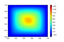
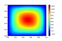
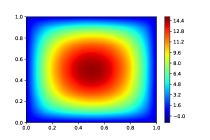
Figure 7: Adaptively learning the Poisson’s equation (symmetric boundary condition).
Left to right: Solution after training layer $L=2$; Solution after training layer $L=3$; Solution after training layer $L=7$

Table 1: Relative $L^{2}$ error on layer addition

Layer No.	$\delta$	$\alpha$	$l_{r}$	Relative $L^{2}$ error
2	10	0.001	0.001	$1.723\times 10^{-1}$
3	15	0.001	0.001	$2.254\times 10^{-2}$
4	20	0.003	0.0005	$4.974\times 10^{-3}$
5	25	0.005	0.0005	$6.649\times 10^{-4}$
6	30	0.05	0.0005	$2.660\times 10^{-4}$
7	35	0.05	0.0001	$6.72\times 10^{-5}$

Table 2: $\%$ of non-zero parameters in each layer

Layer No.	$\%$ of non-zero parameters
2	99.5 $\%$
3	97.7 $\%$
4	98.9 $\%$
5	95.4 $\%$
6	92.5 $\%$
7	96.7 $\%$

Table 3: Performance of Baseline Network and other layerwise training methods (Symmetric boundary condition)

Method	Relative $L^{2}$ error	Parameters trained
		simultaneously
Proposed method	$6.7\times 10^{-5}$	$10,501$
Baseline network	$1.0\times 10^{-4}$	$61,001$
Forward Thinking [9]	$9.2\times 10^{-2}$	$10,501$

F.2 PIANN (slit in the domain)

The solution to this problem suffers from “corner singularity” caused by the nature of the domain [37]. The relative $L^{2}$ error after adding each layer is shown in Table 5. The active parameters in each hidden layer is shown in Table 5. The evolution of solution on adding layers is shown in Figure 4.

Table 4: Relative $L^{2}$ error on layer addition

Layer No.	$\delta$	$\alpha$	$l_{r}$	Relative $L^{2}$ error
2	5	0.001	0.001	$3.59\times 10^{-1}$
3	10	0.001	0.001	$4.75\times 10^{-2}$
4	15	0.005	0.0005	$1.13\times 10^{-3}$
5	20	0.01	0.0005	$7.86\times 10^{-5}$

Table 5: $\%$ of non-zero parameters in each layer

Layer No.	$\%$ of non-zero parameters
2	97.52 $\%$
3	91.29 $\%$
4	97.35 $\%$
5	90.00$\%$

Table 6: Performance of Baseline Network and other layerwise training methods (Slit in domain)

Method	Relative $L^{2}$ error	Parameters trained
		simultaneously
Proposed method	$7.8\times 10^{-5}$	$10,501$
Baseline network	$1.1\times 10^{-4}$	$40,801$
Forward Thinking [9]	$1.6\times 10^{-2}$	$10,501$

F.2.1 From layerwise training to transfer learning for solving PDE’s

Consider the Darcy flow equation given by:

$$-\nabla.(a(x_{1},\ x_{2})\nabla y) =f(x_{1},x_{2})\ \ \ in\ \ \Omega\subset{\mathbb{R}}^{2}$$ (39)

$$y =0\hskip 28.45274ptin\ \ \partial{\mathcal{D}}$$

Traditionally, if one needs to solve Eq. 39 for a different choice of $a(x_{1},x_{2})$ or if new training data is available, the entire training process needs to be repeated for model correction and incurs heavy computational cost. However, in the present case, interpretability of each hidden layer allows us to quickly devise an interpretable transfer learning strategy to alleviate this problem. For demonstration, we consider Case b) scenario, i.e slit in the domain problem. We choose $a(x_{1},\ x_{2})=e^{x_{1}+x_{2}}$ and $f=200$ in Eq. 39. We prune the network hidden layers $4,\ 5$ corresponding to Figure 4 and training is started by adding a new hidden layer ($4^{th}$ layer) with the new problem in hand. In this way, one retains the low-frequency modes of the solution in the initial layers and makes correction only in the final layers. The results and the computational efficiency of the proposed method in comparison to a baseline network is shown in Figure 8.

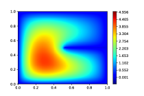
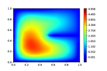
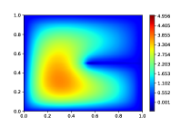
Figure 8: Interpretable transfer learning strategy based on Algorithm 1 to speed up simulations.
First row left to right: True solution; Solution by transfer learning trained for $100$ epochs ($L^{2}$ error= $4.575\times 10^{-3}$); Solution by baseline network trained for $2000$ epochs ($L^{2}$ error= $9.519\times 10^{-3}$).

Appendix G Physics reinforced adaptive neural network (PRANN)

Physics reinforced neural network (PRNN) focus on learning the unknown underlying map by combining sparse noisy measurement data with incomplete/approximate physics [41, 42]. The objective of PRNN is therefore to develop a surrogate model that is consistent with measurement data and constrained by the physical model available.

For demonstration, we consider the problem of learning the electrostatic potential $\psi$ over a domain $\Omega=(0,\ 1)\times(0,\ 1)$ [43]. Noise contaminated measurement data is synthetically generated over $\Omega_{m}=(0.4,\ 0.6)\times(0.4,\ 0.6)$ based on the Poisson equation in Eq. 39 with charge distribution of the form [43]:

$$f(x_{1},\ x_{2})=50\times\left[\sum_{k=1}^{4}(-1)^{k+1}2k\sin{(k\pi x_{1})}\sin{(k\pi x_{2})}\right]+25\times\left(\cos{(2\pi x_{1})}\cos{(2\pi x_{2})}\right)$$ (40)

The training data consists of $1000$ data points on $\Omega_{m}$ and $4000$ data points on $\partial\Omega$. A baseline neural network trained purely on the measurement data cannot capture the solution accurately over the entire domain. The loss function for traditional PRNN has the following form [41]:

$${\mathcal{L}}_{PRNN}(\vec{\theta},\ \omega_{1},\ \omega_{2},\ \omega_{3})=\omega_{1}{\mathcal{L}}_{PDE}(\vec{\theta},\ X_{PDE})+\omega_{2}{\mathcal{L}}_{BC}(\vec{\theta},\ X_{BC})+\omega_{3}{\mathcal{L}}_{data}(\vec{\theta},\ X_{data})$$ (41)

where, ${\mathcal{L}}_{PDE}$ represents the PDE residual loss (mean square error loss), ${\mathcal{L}}_{BC}$ represents the boundary condition loss, and ${\mathcal{L}}_{data}$ represents the data loss. In practise, the hyper-parameter $\omega_{i}$ is often tuned in the middle of training process and the learning is often unstable due to huge list of parameters [41].

In the present approach, neural network learns the boundary conditions through $X_{data}$ which contains a combination of measurement data on $\Omega_{m}$ and data points on $\partial\Omega$. Therefore, only one parameter $\delta=\omega_{1}$ is required in the framework and choosing $\delta$ reflects our confidence in the physical model relative to the measurement data [41]. This translates to the following general problem of achieving a surrogate model parameterized by $\vec{\theta}$ such that:

$$\vec{\theta}^{*}= \arg\min_{\vec{\theta}}{\mathcal{L}}_{PRNN}(\vec{\theta},\ \delta)$$ (42)

$$s.\ t.\ {\mathcal{L}}_{data}(\vec{\theta}^{*}) =\delta_{c}\implies{\mathcal{L}}_{PRNN}(\vec{\theta}^{*},\ \delta)-\delta_{c}=\delta{\mathcal{L}}_{PDE}(\vec{\theta}^{*})$$

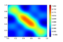
Figure 9: Adaptively learning the solution (PRANN) by Algorithm 1.
First row left to right: Solution after training layer $L=2$; Solution after training layer $L=3$; Solution after training layer $L=4$. Second row left to right: Solution after training layer $L=5$; Solution after training layer $L=6$; Solution after training layer $L=7$

A special case of Eq. 42 follows if in addition one chooses ${\mathcal{L}}_{PDE}(\vec{\theta}^{*})=\delta_{c}$, i.e equal confidence in the physical model and the measurement data [41].

In the proposed approach we embark on a “prediction-updation" strategy where the solution is updated while adding more layers, retaining the previous solution. This is achieved by varying $\delta$ as one adds a new hidden layers and the magnitude of variation is determined automatically based on the output of previous layer. Since $\delta^{i+1}\neq\delta^{i}$, the newly added hidden layer is trainable (Proposition 1).

Performance of layerwise training Algorithm 1

It is to be noted that in reality one only has limited knowledge on the charge distribution. Therefore, the physics loss is computed based on an assumed charge distribution which has the form:

$$f_{a}(x_{1},\ x_{2})=50\times\left[\sum_{k=1}^{4}(-1)^{k+1}2k\sin{(k\pi x_{1})}\sin{(k\pi x_{2})}\right]$$ (43)

For the present problem, we choose $\delta_{c}=1$ in Eq. 42. Inputs chosen for Algorithm 1 is given in Appendix J. The contribution of different terms in the loss function is shown in Table 8. On adding a new layer, $\delta^{i+1}$ is updated following a random walk model:

$$\delta^{i+1}=\delta^{i}+h\times sgn(\delta_{c}-x_{i})\Big{|}\mathcal{N}(0,|x_{i}-\delta_{c}|)\Big{|}$$ (44)

where, $x_{i}$ represents the data loss at the $i^{th}$ step and $h$ is chosen as $1000$. This model ensures that when the predictions of a particular hidden layer produces a high physics loss (Table 8, Figure 9), $\delta$ is increased while training the next hidden layer and the solution is updated to bring down the physics loss. The procedure is then continued till the termination criteria is satisfied. The active parameters in each layer is shown in the Table 8.

Table 7: Contribution of different terms to the loss on adding layers

Layer No.	$\delta$	Data loss	Physics loss
2	290	0.67	0.023
3	960	2.64	0.011
4	670	1.65	0.011
5	480	1.15	0.012
6	380	0.92	0.013
7	430	0.99	0.012

Table 8: $\%$ of non-zero parameters in each layer

Layer No.	$\%$ of non-zero parameters
2	98.17 $\%$
3	96.44 $\%$
4	97.12 $\%$
5	93.84 $\%$
6	96.00 $\%$
7	95.20 $\%$

One of the key advantage of this approach is the interpretability of different hidden layers. For instance, it is clear from Table 8 that layers $3$ and $4$ pays more attention on the physics whereas layers $2,\ 6$ and $7$ pays more attention on the data. This information could be utilized for devising meaningful model updating strategies when new data is available or confidence in the physical model relative to the data changes.

Appendix H Adaptive learning of stable inverse maps from sparse data

Inverse problems are usually ill-posed and involves learning the map from low-dimensional space (observation space) to a high dimensional space (parameter space). This pose a challenge for learning the inverse map especially in the low data regime. It is desirable for the inverse map to be well-posed where the solution’s behaviour should change continuously with respect to input. Therefore, it is clear that the notion of stability defined in proposition 2 is closely related to well-posedness. In fact, enforcing stability imposes well-posedness. Therefore, the developed procedure serves as a natural candidate for this problem.

In this section, we demonstrate the approach for conductivity coefficient field inversion in a 2D heat equation written as:

$$-\nabla\cdot\left(e^{u}\nabla y\right) =20\quad\text{in }\Omega=\left[0,1\right]^{2},$$ (45)

$$y =0\quad\text{ on }\Gamma^{\text{ext}},$$

$$\textbf{n}\cdot\left(e^{u}\nabla y\right) =0\quad\text{ on }\Gamma^{\text{root}},$$

where n is normal vector on the equivalent boundary surfaces. The parameter of interest is denoted as $u$ and the observables are 10 pointwise values of the heat state, $\mathbf{y}$ at arbitrary location. The training data is generated by drawing parameter samples as:

$$\mathbf{u}(\mathbf{x})=\sum_{i=1}^{n}\sqrt{\lambda_{i}}\ \mathbf{\phi}_{i}\ x_{i}$$ (46)

where $\lambda_{i},\ \mathbf{\phi}_{i}$ is the eigen-pair of an exponential two point correlation function and $\textbf{x}=\left(x_{1},\ldots,x_{n}\right)$ is drawn from standard Gaussian distribution [44]. Note that x represents the output of the network. For the present study, we choose the output dimension $n=12$. The observation vector (input of the network) is generated by solving Eq. 45. $5\%$ additive Gaussian noise is added to the observations to represent field condition.

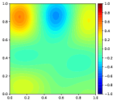
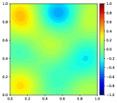
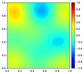
Figure 10: Predicted parameter field for a particular test observation sample using different methods (trained with 50 data sets).
First row left to right: Solution obtained by equivalent baseline network; Exact solution; Solution obtained by Algorithm 1.

Table 9: Relative error achieved by baseline network and other methods

Training data size	Equivalent	Regularized	Proposed method	Forward thinking [9]
	baseline	baseline
20	$0.64$	$0.64$	0.585	1.41
50	0.44	0.44	0.42	0.84

We consider experiments with two different training data size; $20$ and $50$. The validation data set consists of $20$ data points and the test set contains $500$ data points. For evaluating the manifold regularization term, we assume that each input data point (observation) lies in a different manifold, i.e $\mathbf{x}_{m}\in{\mathcal{M}}_{m}$. Each manifold ${\mathcal{M}}_{m}$ is then populated with $100$ artificial perturbations of the input $\mathbf{x}_{m}$.

For this problem, the manifold regularization weight $\gamma$ is doubled while adding a new layer in contrast to other problems, thereby enforcing stability (well-posedness) more strongly in the later layers. This strategy is adopted due to the small data-set size where inital layers should be only weakly regularized allowing for maximum information transfer through the initial layer. However, the data loss increases on adding a new layer in this case. Therefore, the termination criteria in Algorithm 1 is based on the maximum allowable increase in the data loss $\eta^{L}$. Further, by proposition 1, training does not saturate since $\gamma^{i+1}=2\times\gamma^{i}$ and hence one does not require Algorithm 2.

The relative error achieved by different methods is shown in Table 9 which clearly shows that Algorithm 1 outperforms traditional methods. Figure 10 also shows that the parameter field predicted by the proposed method is better than the one produced by baseline network. Further, summary of the adaptive inversion strategy is shown in Figure 11.

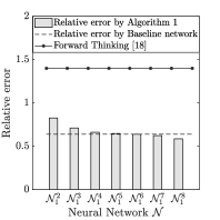
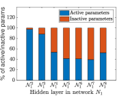
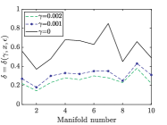
Figure 11: Summary of adaptive inversion (trained with 20 data set).
Left to right: Summary of Algorithm 1; Active and inactive parameters in each hidden layer; Verification of proposition 2.

In order to verify proposition 2, we consider three different models $f_{1},\ f_{2},\ \ f_{3}$ trained exactly in the same way with the same architecture but with different $\gamma$. A training point $\mathbf{x}_{m}\in{\mathcal{M}}_{m}$ is chosen and $5000$ different points $x^{\prime}_{i}\in B_{\varepsilon}(x)$ is artificially generated by perturbing the input $\mathbf{x}_{m}$. Then, $\delta_{k}$ corresponding to model $f_{k}$ can be approximately computed as:

$$\delta_{k}=\max_{i}\Big{(}\left\|f_{k}\left(x\right)-f_{k}\left(x^{\prime}_{i}\right)\right\|_{2}\Big{)}$$ (47)

Figure 11 shows that as $\gamma$ is increased, $\delta$ decreases and provides a feasible way to enforce $\varepsilon-\delta$ stability. Further, Figure 11 shows that indeed $\delta=\delta(\gamma,\ x)$.

Even in this case, the interpretability of hidden layers could be exploited for updating the network when new data is available. Note that in this case initial layers extract maximum information (overfits) from the training data while later layers focus on injecting stability to the learnt inverse map.

Appendix I MNIST classification (Additional results)

I.1 Training with 20 neurons in each hidden layer

The learning curve and parameter efficiency for this case is shown in Figure 12. The inputs for this experiment is given in Appendix J. The last $4$ layers of the network produced by Algorithm 1 is pruned before applying Algorithm 2. Table 10 shows the comparison of results with baseline and other layerwise training method.

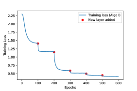
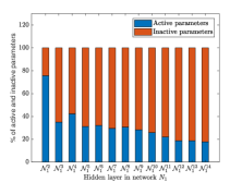
Figure 12: Left to right (20 neurons in each hidden layer): Decrease in training loss with layerwise adaptation; Active and inactive parameters in each hidden layer

Table 10: Performance of baseline network and other layerwise training methods (20 neuron case)

Method	Test Accuracy	Parameters trained
	$\%$	simultaneously
Proposed method	96.90	16,330
Baseline network	96.30	21,370
Regularized baseline	96.30	21,370
Forward Thinking [9]	95.90	16,330

Note that our experiments showed that, forward thinking model [9] quickly over-fits on the training data while adding the initial few layers. Further, forward thinking model is not $\varepsilon-\delta$ stable which is a necessary condition for Algorithm 2 to achieve robustness (Remark 3). Numerically, it is observed that the residual defined in line 4 of Algorithm 2 is very low, and it is hardly possible to extract information from the residual and improve the results. Hence, the performance of forward Thinking model + Algo 2 has been not been included in the comparison results shown in Figure 6 since the behaviour is similar to baseline+Algo 2.

I.2 Training with 500 neurons in each hidden layer

The parameter efficiency and the comparison of results with baseline is shown in Figure 13.

Method Test Params. trained accuracy $\%$ simultaneously Proposed 98.7 $6,48010$ Baseline 98.2 $34,03510$ Regularized baseline 98.3 $34,03510$ Forward Thinking [9] 98.3 $6,48010$

Figure 13: Left to right: Percentage of parameters that are active in each hidden layer; Performance of Baseline Network and other layerwise training methods (case with 500 neurons in hidden layers).

Appendix J Details of input parameter values for different problems

The description of each problem is given below:

I $$:\text{Boston house price prediction problem}$$

II (a) $$:\text{Physics informed adaptive neural network (PIANN), Poisson Equation with symmetric boundary condition}.$$

II (b) $$:\text{Physics informed adaptive neural network (PIANN), Poisson Equation with a Slit in the Domain}.$$

III $$:\text{Physics reinforced adaptive neural network (PRANN).}$$

IV (a) $$:\text{Adaptive learning for inverse problems (20 data-set problem).}$$

IV (B) $$:\text{Adaptive learning for inverse problems (50 data-set problem).}$$

V (a) $$:\text{MNIST classification (20 neuron in hidden layers).}$$

V (b) $$:\text{MNIST classification (500 neuron in hidden layers).}$$

Table 11: Details of input parameters in Algorithm 1 for different problems

Problem	$\varepsilon_{\eta}$	$\rho$	$(\alpha_{0},\delta,\gamma_{0})$	$l_{r}$	$d_{l}$	$E_{e}$	$o$	Batch size
II(a)	$0.035$	$10^{-6}$	$(0.05,\ 0,\ 0.06)$	$0.001$	$0.9$	$50$	$100$	$70$
II (a)	$0.8$	$10^{-6}$	$(v,\ v,\ 0)$	$v$	$1$	$1000$	$100$	$500$
II (b)	$0.5$	$10^{-6}$	$(v,\ v,\ 0)$	$v$	$1$	$2000$	$100$	$500$
III(a)	-	$10^{-6}$	$(0.0001,\ v,\ 0.001)$	$0.001$	$1$	$500$	$100$	$500$
IV (a)	0.035	$10^{-6}$	$(0.0001,\ 0,\ 0.001)$	$0.001$	$1$	$400$	$100$	$20$
IV (b)	0.0015	$10^{-6}$	$(0.0001,\ 0,\ 0.001)$	$0.001$	$1$	$400$	$100$	$50$
V (a)	$0.005$	$10^{-6}$	$(0.001,\ 0,\ 0.0035)$	$0.001$	$0.9$	$100$	$20$	$900$
V (b)	$0.005$	$10^{-6}$	$(0.001,\ 0,\ 0.005)$	$0.001$	$0.9$	$100$	$500$	$900$

where, $v$ represents variable parameter values for different layers.

Table 12: Details of input parameters in Algorithm 2 for different problems

Problem	$\varepsilon_{e}$	$N_{n}$	Architecture	Activation	No of hidden layers	No of hidden neurons
II(a)	$0.1$	$5$	Fully connected	relu	$1$	$10$
V (a)	$0.05$	$20$	Fully connected	elu	$2$	$20$
V (b)	$0.05$	$4$	Fully connected	elu	$2$	$500$

References

- [1] Dan Ellis and Nelson Morgan. Size matters: An empirical study of neural network training for large vocabulary continuous speech recognition. In 1999 IEEE International Conference on Acoustics, Speech, and Signal Processing. Proceedings. ICASSP99 (Cat. No. 99CH36258), volume 2, pages 1013–1016. IEEE, 1999.
- [2] Geoffrey E Hinton. Learning multiple layers of representation. Trends in cognitive sciences, 11(10):428–434, 2007.
- [3] Yann LeCun, Yoshua Bengio, et al. Convolutional networks for images, speech, and time series. The handbook of brain theory and neural networks, 3361(10):1995, 1995.
- [4] Grégoire Montavon, Klaus-Robert Müller, and Mikio Braun. Layer-wise analysis of deep networks with gaussian kernels. Advances in neural information processing systems, 23:1678–1686, 2010.
- [5] Cheng-Yaw Low, Jaewoo Park, and Andrew Beng-Jin Teoh. Stacking-based deep neural network: deep analytic network for pattern classification. IEEE transactions on cybernetics, 50(12):5021–5034, 2019.
- [6] Barret Zoph and Quoc V Le. Neural architecture search with reinforcement learning. arXiv preprint arXiv:1611.01578, 2016.
- [7] Kenneth O Stanley and Risto Miikkulainen. Evolving neural networks through augmenting topologies. Evolutionary computation, 10(2):99–127, 2002.
- [8] Dongxin Xu and Jose C Principe. Training mlps layer-by-layer with the information potential. In IJCNN’99. International Joint Conference on Neural Networks. Proceedings (Cat. No. 99CH36339), volume 3, pages 1716–1720. IEEE, 1999.
- [9] Chris Hettinger, Tanner Christensen, Ben Ehlert, Jeffrey Humpherys, Tyler Jarvis, and Sean Wade. Forward thinking: Building and training neural networks one layer at a time. arXiv preprint arXiv:1706.02480, 2017.
- [10] Mandar Kulkarni and Shirish Karande. Layer-wise training of deep networks using kernel similarity. arXiv preprint arXiv:1703.07115, 2017.
- [11] Saikat Chatterjee, Alireza M Javid, Mostafa Sadeghi, Partha P Mitra, and Mikael Skoglund. Progressive learning for systematic design of large neural networks. arXiv preprint arXiv:1710.08177, 2017.
- [12] Xueli Xiao, Thosini Bamunu Mudiyanselage, Chunyan Ji, Jie Hu, and Yi Pan. Fast deep learning training through intelligently freezing layers. In 2019 International Conference on Internet of Things (iThings) and IEEE Green Computing and Communications (GreenCom) and IEEE Cyber, Physical and Social Computing (CPSCom) and IEEE Smart Data (SmartData), pages 1225–1232. IEEE, 2019.
- [13] Huu-Thiet Nguyen, Chien Chern Cheah, and Kar-Ann Toh. An analytic layer-wise deep learning framework with applications to robotics. arXiv preprint arXiv:2102.03705, 2021.
- [14] Diego Rueda-Plata, Raúl Ramos-Pollán, and Fabio A González. Supervised greedy layer-wise training for deep convolutional networks with small datasets. In Computational Collective Intelligence, pages 275–284. Springer, 2015.
- [15] Eugene Belilovsky, Michael Eickenberg, and Edouard Oyallon. Greedy layerwise learning can scale to imagenet. In International conference on machine learning, pages 583–593. PMLR, 2019.
- [16] Régis Lengellé and Thierry Denoeux. Training mlps layer by layer using an objective function for internal representations. Neural Networks, 9(1):83–97, 1996.
- [17] Yoshua Bengio, Pascal Lamblin, Dan Popovici, Hugo Larochelle, et al. Greedy layer-wise training of deep networks. Advances in neural information processing systems, 19:153, 2007.
- [18] Lemeng Wu, Dilin Wang, and Qiang Liu. Splitting steepest descent for growing neural architectures. Advances in Neural Information Processing Systems, 32, 2019.
- [19] Mike Wynne-Jones. Node splitting: A constructive algorithm for feed-forward neural networks. Neural Computing & Applications, 1(1):17–22, 1993.
- [20] Tianqi Chen, Ian Goodfellow, and Jonathon Shlens. Net2net: Accelerating learning via knowledge transfer. arXiv preprint arXiv:1511.05641, 2015.
- [21] Loc Quang Trinh. Greedy layerwise training of convolutional neural networks. PhD thesis, Massachusetts Institute of Technology, 2019.
- [22] Benjamin A Clegg, Gregory J DiGirolamo, and Steven W Keele. Sequence learning. Trends in cognitive sciences, 2(8):275–281, 1998.
- [23] Mikhail Belkin, Partha Niyogi, and Vikas Sindhwani. Manifold regularization: A geometric framework for learning from labeled and unlabeled examples. Journal of machine learning research, 7(11), 2006.
- [24] Maziar Raissi, Paris Perdikaris, and George E Karniadakis. Physics-informed neural networks: A deep learning framework for solving forward and inverse problems involving nonlinear partial differential equations. Journal of Computational Physics, 378:686–707, 2019.
- [25] Kaiming He, Xiangyu Zhang, Shaoqing Ren, and Jian Sun. Deep residual learning for image recognition. In Proceedings of the IEEE conference on computer vision and pattern recognition, pages 770–778, 2016.
- [26] Kaiming He, Xiangyu Zhang, Shaoqing Ren, and Jian Sun. Identity mappings in deep residual networks. In European conference on computer vision, pages 630–645. Springer, 2016.
- [27] Farkhondeh Kiaee, Christian Gagné, and Mahdieh Abbasi. Alternating direction method of multipliers for sparse convolutional neural networks. arXiv preprint arXiv:1611.01590, 2016.
- [28] Wei Wen, Chunpeng Wu, Yandan Wang, Yiran Chen, and Hai Li. Learning structured sparsity in deep neural networks. arXiv preprint arXiv:1608.03665, 2016.
- [29] Charles Jin and Martin Rinard. Manifold regularization for locally stable deep neural networks. arXiv preprint arXiv:2003.04286, 2020.
- [30] Djork-Arné Clevert, Thomas Unterthiner, and Sepp Hochreiter. Fast and accurate deep network learning by exponential linear units (elus). arXiv preprint arXiv:1511.07289, 2015.
- [31] Henry Gouk, Eibe Frank, Bernhard Pfahringer, and Michael J Cree. Regularisation of neural networks by enforcing lipschitz continuity. Machine Learning, 110(2):393–416, 2021.
- [32] David Harrison Jr and Daniel L Rubinfeld. Hedonic housing prices and the demand for clean air. Journal of environmental economics and management, 5(1):81–102, 1978.
- [33] Mohsen Shahhosseini, Guiping Hu, and Hieu Pham. Optimizing ensemble weights for machine learning models: A case study for housing price prediction. In INFORMS International Conference on Service Science, pages 87–97. Springer, 2019.
- [34] James MacQueen et al. Some methods for classification and analysis of multivariate observations. In Proceedings of the fifth Berkeley symposium on mathematical statistics and probability, volume 1, pages 281–297. Oakland, CA, USA, 1967.
- [35] Maithra Raghu, Ben Poole, Jon Kleinberg, Surya Ganguli, and Jascha Sohl-Dickstein. On the expressive power of deep neural networks. In international conference on machine learning, pages 2847–2854. PMLR, 2017.
- [36] Han Gao, Matthew J Zahr, and Jian-Xun Wang. Physics-informed graph neural galerkin networks: A unified framework for solving pde-governed forward and inverse problems. Computer Methods in Applied Mechanics and Engineering, 390:114502, 2022.
- [37] Bing Yu et al. The deep ritz method: a deep learning-based numerical algorithm for solving variational problems. arXiv preprint arXiv:1710.00211, 2017.
- [38] Jian Li, Yong Liu, Rong Yin, and Weiping Wang. Approximate manifold regularization: Scalable algorithm and generalization analysis. In IJCAI, pages 2887–2893, 2019.
- [39] Mikhail Belkin and Partha Niyogi. Towards a theoretical foundation for laplacian-based manifold methods. Journal of Computer and System Sciences, 74(8):1289–1308, 2008.
- [40] Diederik P Kingma and Jimmy Ba. Adam: A method for stochastic optimization. arXiv preprint arXiv:1412.6980, 2014.
- [41] Minglang Yin, Xiaoning Zheng, Jay D Humphrey, and George Em Karniadakis. Non-invasive inference of thrombus material properties with physics-informed neural networks. Computer Methods in Applied Mechanics and Engineering, 375:113603, 2021.
- [42] Shengze Cai, Zhiping Mao, Zhicheng Wang, Minglang Yin, and George Em Karniadakis. Physics-informed neural networks (pinns) for fluid mechanics: A review. Acta Mechanica Sinica, pages 1–12, 2022.
- [43] Shaan Desai, Marios Mattheakis, Hayden Joy, Pavlos Protopapas, and Stephen Roberts. One-shot transfer learning of physics-informed neural networks. arXiv preprint arXiv:2110.11286, 2021.
- [44] Paul G Constantine, Carson Kent, and Tan Bui-Thanh. Accelerating markov chain monte carlo with active subspaces. SIAM Journal on Scientific Computing, 38(5):A2779–A2805, 2016.