Reconciling cosmic dipolar tensions with a gigaparsec void

Abstract

Recent observations indicate a $4.9\sigma$ tension between the CMB and quasar dipoles. This tension challenges the cosmological principle. We propose that if we live in a gigaparsec scale void, the CMB and quasar dipolar tension can be reconciled. This is because we are unlikely to live at the center of the void. And a 15% offset from the center will impact the quasars and CMB differently in their dipolar anisotropies. As we consider a large and thick void, our setup can also ease the Hubble tension.

Introduction – The cosmological principle is a fundamental postulate in modern cosmology, assuming that the Universe is homogeneous and isotropic on large scales, independent of location of observers 1937RSPSA.158..324M . Based on the cosmological principle, the Lambda cold dark matter ($\Lambda\mathrm{CDM}$) model 1970ApJ…159..379R ; PhysRevLett.52.2090 ; 1985Natur.317..595F is established and considered as the standard model of cosmology.

With the development of precision cosmology, new observable results show hints of inconsistencies between observations and the cosmological principle, e.g., the detection of cosmic dipole such as cosmic microwave background (CMB) dipole Planck:2018nkj and quasar dipole Secrest:2020has may be inconsistent and indicate an anisotropic observable universe. Also, the Hubble tension between its local measurements Riess:2016jrr ; Brout:2022vxf and the value from Planck Planck:2016kqe , which may be interpreted as the existence of a local inhomogeneous structure Ding:2019mmw ; Haslbauer:2020xaa . A fundamental explanation is needed in these problems.

In reconciling the inconsistency between observations and the cosmological principle, a number of models have been proposed, such as introducing new physical scenarios in solving the Hubble tension Poulin:2018cxd ; Bernal:2016gxb ; Agrawal:2019lmo ; Lin:2019qug ; Kenworthy:2019qwq ; Vagnozzi:2019ezj ; Fung:2021fcj and using the peculiar motion of observers in explaining the cosmic dipole 1984MNRAS.206..377E ; Lavaux:2008th . However, the tension between the CMB dipole and quasar dipole remains unsolved. The amplitude of the quasar dipole is over twice as large as the expected value in kinematic interpretation of the CMB dipole. This inconsistency has $4.9\sigma$ significance Secrest:2020has . Such a large quasar dipole anisotropy still exists after removing the standard kinematic dipole in CMB frame, which may indicate the existence of a local anisotropic structure Secrest:2022uvx .

The introduction of a Gpc-scale local void changes the story. A local underdense region with us as observers inside could cause the detection of obvious peculiar motion of nearby supernovae (SNe). A Gpc-scale void makes sure that almost all detected SNe live inside, which biases local measurement of Hubble parameter and ease the Hubble tension (see Ding:2019mmw for more details). Since it is very unlikely for the position of the Milky Way to locate at the exact center of this local void, the observational anisotropy would be induced by an off-center location of observers inside the void Alnes:2006pf ; Alnes:2006uk ; Nistane:2019yzd .

In this Letter, we propose that the amplitude inconsistency between CMB and quasar dipoles can also be explained by our offset from the center of a void. Due to the existence of such an anisotropic spacetime in an off-center void, the detected photons from different directions have experienced different cosmic expansion histories, which causes an anisotropy in their cosmic redshifts. The CMB dipole and quasar dipole, measured from CMB temperature perturbations and hemisphere quasar number counting Rameez:2017euv respectively, could also be in part attributed to the redshift dipole anisotropy. Since the redshift dipole is induced by anisotropic matter distribution inside the void, it reaches a peak value at the boundary of the void. Thus, by considering that we live at an off-center position of a void, the origin of the quasar dipole can be explained, where the void has thick boundary and is as large as the average distance from us to distant quasars. We also provide a first-principle calculation of the intrinsic matter density dipole anisotropy in an off-center local void scenario, which is the origin of the detected cosmic dipole and has a similar behavior to the redshift dipole.

Origin – In standard cosmological scenarios where structures originate from a Gaussian random density field, the presence of a Gpc-scale void is unlikely, due to $\sigma_{8}\simeq 0.81$ Planck:2018vyg , which shows that the amplitude of fluctuations is statistically suppressed on comoving scales much larger than $10~{}\mathrm{Mpc}$. Therefore, a Gpc-scale void, if exists, deserves a distinct primordial origin. Multi-stream inflation Li:2009sp is a potential mechanism to produce a Gpc-scale void. Multi-stream inflation can also generate position space features in cosmology, such as multiverse structures Li:2009me , CMB cold spot Afshordi:2010wn , initial primordial black holes clustering Ding:2019tjk , and primordial stellar bubbles Cai:2021zxo .

In multi-stream inflation, the inflationary trajectory may encounter a barrier, and then bifurcates into two paths, which experience different inflationary potentials. The inflationary dynamics and the void profile is related as follows: (i) The density contract between in and outside the void is determined by the e-folding number difference between the two trajectories. The trajectory which is now a void has less e-folds of inflation, by $\delta\rho/\rho\sim\delta N$, where $\delta N$ is the e-folding number difference. (ii) The size of the void is determined by the comoving scale during inflation when bifurcation happened. Thus, the size of the void is a free parameter which can be made Gpc. (iii) The thickness of the boundary between inside and outside the void is determined by the combination scale of the two trajectories Ding:2019mmw . Thus, the void originated from multi-stream inflation can have a smooth profile, which is very important for our model to be consistent with kSZ constraints, as we will emphasize later.

Observational constraints – The existence of such a Gpc-scale void affects different observations of e.g. Type Ia SNe, baryon acoustic oscillations (BAO) and CMB. The cosmic influence of a void with suitable profile should be consistent with these observational constraints. We briefly review results in Ding:2019mmw about how observations constrain such a void (see also Biswas:2010xm and references therein).

Type Ia SNe provide a key measurement for the local Universe. From their light curves at redshift $0<z<2.3$ Scolnic:2021amr , the luminosity distance-redshift relation can be determined, which gives a local Hubble parameter $H_{0}=73.3\pm 1.1\mathrm{km}~{}\mathrm{s}^{-1}~{}\mathrm{Mpc}^{-1}$ in $\Lambda\mathrm{CDM}$ cosmology Brout:2022vxf , while Planck gives Hubble parameter $H_{0}=66.9\pm 0.6\mathrm{km}~{}\mathrm{s}^{-1}~{}\mathrm{Mpc}^{-1}$ Planck:2016kqe . Such a tension in Hubble parameter could be eased by a local Gpc-scale void with the Milky Way inside, which cause nearby SNe to live inside the void and have significant positive peculiar velocities, biasing local measurement of Hubble parameter.

BAO scale measurements at different redshifts 2011MNRAS.416.3017B ; Ross:2014qpa ; BOSS:2016wmc ; Planck:2018vyg are standard rulers from local Universe to primordial Universe. Through a model-independent observable $(\Delta\theta^{2}\Delta z)^{1/3}$, cosmological models could be constrained. Compared with the flat FRW model, the spatial curvature in the local void biases a lager $(\Delta\theta^{2}\Delta z)^{1/3}$, which fits the observational data better Ding:2019mmw ; Biswas:2010xm .

A local void could cause the temperature perturbation at small scales of CMB, due to interactions between bulk flow electrons and CMB photons, which is called the kinetic Sunyaev-Zel’dovich (kSZ) effect Hoscheit:2018nfl . The power spectrum $C_{\ell}$ at $\ell=3000$ puts strong constraints on void profiles, which forbids a Gpc-scale void to have a significant depth. Such a constraint could be eased by increasing the width of the void boundary. Bulk flow electrons in a thick edge void have smaller peculiar velocity than that in a sharp edge void. Therefore, collisions between bulk flow electrons and CMB photons produce weaker temperature distortions in CMB spectrum, which is shown in Fig. 1.

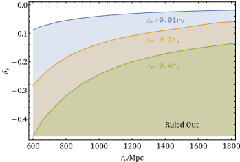
Figure 1: The kSZ constraints on void profiles, see also Ding:2019mmw . $\delta_{V}$ is the matter density contrast, $r_{V}$ is void radius and $\Delta_{r}$ is the thickness of the void boundary. The shadow regions are ruled out parameter regions with boundary thicknesses $\Delta_{r}/r_{V}=0.01,0.1,0.4$. We observe that voids with thicker boundaries are significantly less constrained by the kSZ effect.

Cosmic dipoles – In following part, we focus on the CMB dipole and quasar dipole induced by the off-center observation inside a Gpc-scale void. The void is modeled by the Lemaitre-Tolman-Bondi (LTB) metric

$$\mathrm{d}s^{2}=c^{2}\mathrm{d}t^{2}-\frac{R^{\prime}(r,t)^{2}}{1-k(r)}\mathrm{d}r^{2}-R^{2}(r,t)\mathrm{d}\Omega^{2}~{},$$ (1)

where $R^{\prime}(r,t)=\partial R(r,t)/\partial r$. The Friedmann equation is then

$$\frac{H(r,t)^{2}}{H_{0}(r)^{2}}=\Omega_{M}(r)\frac{R_{0}(r)^{3}}{R(r,t)^{3}}+\Omega_{k}(r)\frac{R_{0}(r)^{2}}{R(r,t)^{2}}+\Omega_{\Lambda}(r)~{}.$$ (2)

Here, the spacetime-dependent local Hubble parameter can be calculated as $H(r,t)=\dot{R}(r,t)/R(r,t)$ and $H_{0}(r)\equiv H(r,t_{0})$. $\Omega_{X}(r)\equiv\rho_{X}(r)/\rho_{c}(r)$ with $X=M,k,\Lambda$, representing matter, curvature and dark energy, respectively. The critical energy density is $\rho_{c}(r)\equiv 3H_{0}(r)^{2}/8\pi G$. The density parameters satisfy $\Omega_{M}(r)+\Omega_{k}(r)+\Omega_{\Lambda}(r)=1$.

The profile of a local void is defined as $\delta(r)\equiv\rho_{M}(r)/\rho_{M}(\infty)-1$. We follow Kenworthy:2019qwq to parameterize the void profile as

$$\delta(r)=\delta_{V}\frac{1-\tanh((r-r_{V})/2\Delta_{r})}{1+\tanh(r_{V}/2\Delta_{r})}~{},$$ (3)

where $\delta_{V}$ and $r_{V}$ are the depth and radius of the void, and $\Delta_{r}$ is the width of the void boundary. $R(r,t)$ can be numerically solved (see Ding:2019mmw for more details). In this work, we mainly focus on parameters of the void profile with $r_{V}=3200\mathrm{Mpc}$, $\Delta_{r}=0.18r_{V}$ and $\delta_{V}=-0.057$, which is allowed under the kSZ constraint.

To calculate the dipole signals seen by an off-center observer, it is crucial to specify photon trajectories. Given the position of the observer and the direction of photon arrival as initial conditions, we can numerically solve the geodesic equations of photons backward in time from the present cosmic time to a past cosmic time and obtain the redshift distribution of photons from a constant time hypersurface Alnes:2006pf .

Assuming that the observer is placed in the $z$-axis with distance $d$. For a photon hitting the observer at angle $\xi$ relative to the $z$-axis, the corresponding CMB temperature is then directly related to redshift

$$T(\xi)=\frac{T_{*}}{1+z(\xi)}~{},$$ (4)

where $T_{*}$ is the temperature at the last-scattering surface. Then the relative temperature variation is

$$\Theta(\xi)\equiv\frac{\Delta T}{\widehat{T}}=\frac{T(\xi)-\widehat{T}}{\widehat{T}}~{},$$ (5)

with the average temperature $\widehat{T}=\int\mathrm{d}\Omega\,T(\xi)/4\pi$. Now we can calculate the amplitude of CMB dipole,

$$\mathcal{D}=\frac{2}{\pi}\int^{\pi}_{0}\Theta(\xi)\cos\xi\,\mathrm{d}\xi~{}.$$ (6)

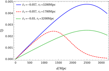
Figure 2: CMB dipole as a function of observer’s location, where $d$ is the distance from the observer to the void center. Different sets of parameters of the void are shown in the labels with the same relative edge width $\Delta_{r}=0.18r_{V}$.

Naturally, the distance from the off-center observer to the center of the void plays an important role. As shown in Fig. 2, the CMB dipole first increases as the observer location becomes further away from the void center, but when the observer passes the void boundary, the dipole reaches its maximum and starts to decrease, which is conceivable since the observer is no longer inside the void. Meanwhile, the void profile is also significant to the observed CMB dipole. Comparing different curves in Fig. 2, the amplitude of the observed CMB dipole is generally smaller for a shallower void and a larger void radius could produce a larger anisotropic region in the Universe. As in the previous setting, we consider the parameter of void profile $(r_{V},\Delta_{r},\delta_{V})=(3.2\mathrm{Gpc},0.6\mathrm{Gpc},-0.057)$. In this benchmark model, the amplitude of detected CMB dipole $\mathcal{D}\simeq 1.23\times 10^{-3}$ Planck:2018nkj corresponds with the location of the observer is $492\mathrm{Mpc}$ away from the center of the void, which we will use in following discussion.

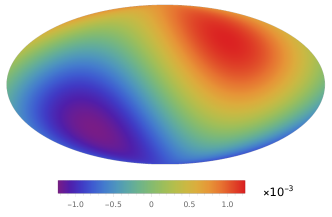
Figure 3: Observed CMB dipole in the view of an off-center observer. The distance of the observer from void center is set to be $492\text{Mpc}$ and the position direction from void center to the observer is set to (264°, 48°) in galactic coordinates, which is coincide with measured CMB dipole direction.

As the LTB metric is isotropic, the orientation of CMB dipole seen by an off-center observer is the same as the direction from the void center to the observer. We can simply set the position direction of the off-center observer to be consistent with CMB dipole, which is $(l,b)=$ (264°, 48°) in galactic coordinate Planck:2018nkj . Fig. 3 shows an example plot of the CMB dipole seen by an observer located 492Mpc from the center.

Note that this method can be extended from CMB where $z=1100$ to cosmic dipoles corresponding to other redshifts, as long as the observable signal is related to redshift in the same way as temperature in Eq.(4). Such dipole relation is shown as the blue curve in Fig. 4, cosmic dipole amplitude reaches maximum around $z=1$, just at the edge of the void. When the source gets away from the void, the amplitude of the dipole becomes stable since the source can be approximately considered to be at infinity.

Besides CMB, distant sources like quasars can also form dipoles in void cosmology. For CMB, the dipole appears in its temperature anisotropy, while for quasar, the dipole appears in number counting anisotropy. That is to say angular number density $\text{d}N/\text{d}\Omega$ is different when observer looks into different direction $\xi$.

Such anisotropy can be derived using similar methods in kinematic interpretation of the quasar dipole 1984MNRAS.206..377E . Consider an off-center observer in a local void, the frequency of observed photons is shifted from the emission frequency as

$$\nu_{\text{o}}=\nu_{\text{e}}\kappa(\xi)~{},$$ (7)

where $\kappa(\xi)=(1+\bar{z})/(1+z(\xi))$, and $\bar{z}$ is the mean redshift. Such an angular-dependent frequency shift is induced by the redshift anisotropy in an off-center void. This causes the anisotropy in power-law spectral energy distribution of the source $S\propto\nu^{-\alpha}$ and a cumulative power-law distribution above a limiting apparent flux density $N(>S)\propto S^{-x}$. The observed solid angle can be approximated to $d\Omega_{o}\simeq d\Omega_{e}\kappa(\xi)^{-2}$ Hogg:1999ad . Accordingly, the observed number angular density is

$$\Big{(}\frac{\text{d}N}{\text{d}\Omega}\Big{)}_{\text{o}}\simeq\Big{(}\frac{\text{d}N}{\text{d}\Omega}\Big{)}_{\text{e}}\kappa(\xi)^{\gamma}~{},$$ (8)

where the index $\gamma=2+x(1+\alpha)$. Following Secrest:2022uvx , we set $\alpha=1.06$, $x=1.89$. The averaged number angular density can be integrated

$$\Big{(}\frac{\text{d}N}{\text{d}\Omega}\Big{)}_{\text{a}}=\frac{1}{4\pi}\int\Big{(}\frac{\text{d}N}{\text{d}\Omega}\Big{)}_{\text{o}}\text{d}\Omega~{}.$$ (9)

The relative variation is

$$\Theta(\xi)=\frac{\Delta(\text{d}N/\text{d}\Omega)}{(\text{d}N/\text{d}\Omega)_{a}}=\frac{(\text{d}N/\text{d}\Omega)_{\text{o}}-(\text{d}N/\text{d}\Omega)_{a}}{(\text{d}N/\text{d}\Omega)_{a}}~{},$$ (10)

then the amplitude of quasar dipole can be calculated as Eq. (6).

Similar to the temperature dipole, the angular number density dipole can be calculated for quasars located at different redshifts shown as the red dashed curve in Fig. 4. It is clear that there is a peak for the dipole anisotropy around $z=1$, due to the existence of a Gpc-scale local void. Therefore, when considering kinematic interpretations of quasar dipoles, such a peak dipole anisotropy induced by an off-center void can cause a larger amplitude in the quasar dipole. This reconciles the peculiar velocity inconsistency between the quasar and CMB dipoles.

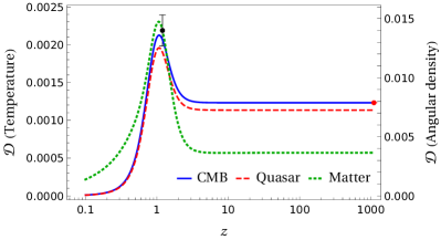
Figure 4: Cosmic dipole as a function of redshift. The observer is located at $492\text{Mpc}$ from the void center. The blue solid curve represents CMB-like temperature dipole while the other two curves represent quasar dipole and angular matter density dipole, denoted by red dashed and green doted curves, respectively. The black data point is the quasar dipole $\mathcal{D}=(1.40\pm 0.13)\times 10^{-2}$ at the mean redshift of quasars $z=1.2$ Secrest:2022uvx and the red data point is the CMB dipole $\mathcal{D}=(1.23\pm 0.00036)\times 10^{-3}$ at redshift $z=1100$ Planck:2018nkj .

In principle, there is an intrinsic matter distribution anisotropy in the view of an off-center observer inside the void and it is the origin of the observed quasar dipole. If we assume that the number density of quasars is determined by their surrounding matter density, the amplitude of quasar dipole should be similar to the amplitude of angular matter density dipole. In calculating angular matter density in a local void, the mass term is the matter density times the observed volume elements and the angular term is the observed solid angle, which can be expressed as follows,

$$\frac{\text{d}M}{\text{d}\Omega}(\xi)\simeq\frac{\rho a^{3}r^{2}\text{d}r\text{d}\Omega}{\text{d}\Omega}=\frac{\rho(\xi)r(\xi)^{2}\text{d}r(\xi)}{[1+z(\xi)]^{3}}~{},$$ (11)

where $a$ is the scale factor corresponding to the observational angle $\xi$. Although $a$ does not appear in the LTB metric we adopt, it is still used during our approximation due to its convenience. Relative variation and dipole amplitude can be therefore calculated as previously discussed. The results are shown as the green dotted curve of Fig. 4.

In Fig. 4, we can see the quasar dipole and angular matter density dipole behave differently with respect to redshift. It is reasonable that the matter distribution anisotropy is the origin of detected quasar dipole, therefore, the anisotropy first appears in the matter distribution, then induces a redshift anisotropy in observable signals from quasars, and the difference between the magnitude of these two dipolar anisotropies is small. Especially, the amplitude of these two dipolar anisotropies takes similar values around $z=1.2$, which is the mean redshift of observed quasars Marocco_2021 . It shows the angular matter density dipole could be a decent approximation to the quasar number dipole.

Conclusions and Remarks – To summarize, we propose that the existence of a Gpc-scale local void could affect the validity of the cosmological principle, and reconciling the related dipolar tension. In particular, we study the induced CMB dipole and quasar dipole in the view of an off-center observer inside a Gpc-scale local void. Due to the intrinsic matter distribution anisotropy in an off-center void, the detected photons from different directions have experienced distinct cosmic expansion histories, which causes an anisotropy in their redshift. Such a redshift anisotropy could induce cosmic dipoles by affecting the CMB temperature fluctuation and the analysis in quasar number counting. In our benchmark void model with a $3.2\mathrm{Gpc}$ void radius, $0.6\mathrm{Gpc}$ void boundary and $-0.057$ density contrast, an off-center observer with $492\mathrm{Mpc}$ away from the void center and relative orientation $(l,b)=$ (264°, 48°) in galactic coordinate, could observe the CMB dipole $\mathcal{D}\simeq 1.23\times 10^{-3}$ and quasar dipole $\mathcal{D}\simeq 1.25\times 10^{-2}$. The larger amplitude of quasar dipole than that of CMB dipole is caused by the peak anisotropy at the boundary of the void around $z=1$ and the dipolar tension between them decreases from $4.9\sigma$ to $1\sigma$ in a Gpc-scale void as shown in Fig. 4.

In this work, motivated by the dipolar tension, we mainly focus on comparing the cosmic dipoles induced by the anisotropy matter distribution in an off-center void. We have not considered the peculiar motion in the local flow, which should affect the CMB and quasar dipoles in the same way and thus does not affect the comparison. Also, we may be moving with respect to the void, which can further extend our model. Finally, if the shape of the void is not spherical, additional anistropies of higher multipoles may also be introduced.

It is also important to note that due to the off-center observer in a void, the dipolar anisotropy should consistently exist in many cosmic signals, e.g., Type Ia SNe Alnes:2006uk ; Sun:2018cha ; Mohayaee:2020wxf , large scale structure Globus:2018svy , $21\mathrm{cm}$ background Cooray:2006km and gravitational wave background NANOGrav:2020bcs . If we are indeed located in a void, the void profile can be understood better by a combined study of these signals.

Acknowledgement – We thank Haipeng An and Zhong-Zhi Xianyu for helpful discussion. This work is supported in part by the National Key R&D Program of China (2021YFC2203100), the NSFC Excellent Young Scientist Scheme (Hong Kong and Macau) Grant No. 12022516, and the GRF grant 16303621 by the RGC of Hong Kong SAR.

References

- (1) E. A. Milne, “Kinematics, Dynamics, and the Scale of Time,” Proc. R. Soc. Lond. Ser. A 158 no. 894, (Jan., 1937) 324–348.
- (2) V. C. Rubin and J. Ford, W. Kent, “Rotation of the Andromeda Nebula from a Spectroscopic Survey of Emission Regions,” Astrophys. J. 159 (Feb., 1970) 379.
- (3) M. S. Turner, G. Steigman, and L. M. Krauss, “Flatness of the universe: Reconciling theoretical prejudices with observational data,” Phys. Rev. Lett. 52 (Jun, 1984) 2090–2093.
- (4) C. S. Frenk, S. D. M. White, G. Efstathiou, and M. Davis, “Cold dark matter, the structure of galactic haloes and the origin of the Hubble sequence,” Nature (London) 317 no. 6038, (Oct., 1985) 595–597.
- (5) Planck Collaboration, N. Aghanim et al., “Planck 2018 results. I. Overview and the cosmological legacy of Planck,” Astron. Astrophys. 641 (2020) A1, arXiv:1807.06205 [astro-ph.CO].
- (6) N. J. Secrest, S. von Hausegger, M. Rameez, R. Mohayaee, S. Sarkar, and J. Colin, “A Test of the Cosmological Principle with Quasars,” Astrophys. J. Lett. 908 no. 2, (2021) L51, arXiv:2009.14826 [astro-ph.CO].
- (7) A. G. Riess et al., “A 2.4% Determination of the Local Value of the Hubble Constant,” Astrophys. J. 826 no. 1, (2016) 56, arXiv:1604.01424 [astro-ph.CO].
- (8) D. Brout et al., “The Pantheon+ Analysis: Cosmological Constraints,” arXiv:2202.04077 [astro-ph.CO].
- (9) Planck Collaboration, N. Aghanim et al., “Planck intermediate results. XLVI. Reduction of large-scale systematic effects in HFI polarization maps and estimation of the reionization optical depth,” Astron. Astrophys. 596 (2016) A107, arXiv:1605.02985 [astro-ph.CO].
- (10) Q. Ding, T. Nakama, and Y. Wang, “A gigaparsec-scale local void and the Hubble tension,” Sci. China Phys. Mech. Astron. 63 no. 9, (2020) 290403, arXiv:1912.12600 [astro-ph.CO].
- (11) M. Haslbauer, I. Banik, and P. Kroupa, “The KBC void and Hubble tension contradict CDM on a Gpc scale Milgromian dynamics as a possible solution,” Mon. Not. Roy. Astron. Soc. 499 no. 2, (2020) 2845–2883, arXiv:2009.11292 [astro-ph.CO].
- (12) V. Poulin, T. L. Smith, T. Karwal, and M. Kamionkowski, “Early Dark Energy Can Resolve The Hubble Tension,” Phys. Rev. Lett. 122 no. 22, (2019) 221301, arXiv:1811.04083 [astro-ph.CO].
- (13) J. L. Bernal, L. Verde, and A. G. Riess, “The trouble with ,” JCAP 10 (2016) 019, arXiv:1607.05617 [astro-ph.CO].
- (14) P. Agrawal, F.-Y. Cyr-Racine, D. Pinner, and L. Randall, “Rock ’n’ Roll Solutions to the Hubble Tension,” arXiv:1904.01016 [astro-ph.CO].
- (15) M.-X. Lin, G. Benevento, W. Hu, and M. Raveri, “Acoustic Dark Energy: Potential Conversion of the Hubble Tension,” Phys. Rev. D 100 no. 6, (2019) 063542, arXiv:1905.12618 [astro-ph.CO].
- (16) W. D. Kenworthy, D. Scolnic, and A. Riess, “The Local Perspective on the Hubble Tension: Local Structure Does Not Impact Measurement of the Hubble Constant,” Astrophys. J. 875 no. 2, (2019) 145, arXiv:1901.08681 [astro-ph.CO].
- (17) S. Vagnozzi, “New physics in light of the tension: An alternative view,” Phys. Rev. D 102 no. 2, (2020) 023518, arXiv:1907.07569 [astro-ph.CO].
- (18) L. W. Fung, L. Li, T. Liu, H. N. Luu, Y.-C. Qiu, and S. H. H. Tye, “The Hubble Constant in the Axi-Higgs Universe,” arXiv:2105.01631 [astro-ph.CO].
- (19) G. F. R. Ellis and J. E. Baldwin, “On the expected anisotropy of radio source counts,” Mon. Not. Roy. Astron. Soc. 206 (Jan., 1984) 377–381.
- (20) G. Lavaux, R. B. Tully, R. Mohayaee, and S. Colombi, “Cosmic flow from 2MASS redshift survey: The origin of CMB dipole and implications for LCDM cosmology,” Astrophys. J. 709 (2010) 483–498, arXiv:0810.3658 [astro-ph].
- (21) N. J. Secrest, S. von Hausegger, M. Rameez, R. Mohayaee, and S. Sarkar, “A Challenge to the Standard Cosmological Model,” Astrophys. J. Lett. 937 no. 2, (2022) L31, arXiv:2206.05624 [astro-ph.CO].
- (22) H. Alnes and M. Amarzguioui, “CMB anisotropies seen by an off-center observer in a spherically symmetric inhomogeneous Universe,” Phys. Rev. D 74 (2006) 103520, arXiv:astro-ph/0607334.
- (23) H. Alnes and M. Amarzguioui, “The supernova Hubble diagram for off-center observers in a spherically symmetric inhomogeneous Universe,” Phys. Rev. D 75 (2007) 023506, arXiv:astro-ph/0610331.
- (24) V. Nistane, G. Cusin, and M. Kunz, “CMB sky for an off-center observer in a local void. Part I. Framework for forecasts,” JCAP 12 (2019) 038, arXiv:1908.05484 [astro-ph.CO].
- (25) M. Rameez, R. Mohayaee, S. Sarkar, and J. Colin, “The dipole anisotropy of AllWISE galaxies,” Mon. Not. Roy. Astron. Soc. 477 no. 2, (2018) 1772–1781, arXiv:1712.03444 [astro-ph.CO].
- (26) Planck Collaboration, N. Aghanim et al., “Planck 2018 results. VI. Cosmological parameters,” Astron. Astrophys. 641 (2020) A6, arXiv:1807.06209 [astro-ph.CO]. [Erratum: Astron.Astrophys. 652, C4 (2021)].
- (27) M. Li and Y. Wang, “Multi-Stream Inflation,” JCAP 07 (2009) 033, arXiv:0903.2123 [hep-th].
- (28) S. Li, Y. Liu, and Y.-S. Piao, “Inflation in Web,” Phys. Rev. D 80 (2009) 123535, arXiv:0906.3608 [hep-th].
- (29) N. Afshordi, A. Slosar, and Y. Wang, “A Theory of a Spot,” JCAP 01 (2011) 019, arXiv:1006.5021 [astro-ph.CO].
- (30) Q. Ding, T. Nakama, J. Silk, and Y. Wang, “Detectability of Gravitational Waves from the Coalescence of Massive Primordial Black Holes with Initial Clustering,” Phys. Rev. D 100 no. 10, (2019) 103003, arXiv:1903.07337 [astro-ph.CO].
- (31) Y.-F. Cai, C. Chen, Q. Ding, and Y. Wang, “Ultrahigh-energy gamma rays and gravitational waves from primordial exotic stellar bubbles,” Eur. Phys. J. C 82 no. 5, (2022) 464, arXiv:2105.11481 [astro-ph.CO].
- (32) T. Biswas, A. Notari, and W. Valkenburg, “Testing the Void against Cosmological data: fitting CMB, BAO, SN and H0,” JCAP 11 (2010) 030, arXiv:1007.3065 [astro-ph.CO].
- (33) D. Scolnic et al., “The Pantheon+ Analysis: The Full Dataset and Light-Curve Release,” arXiv:2112.03863 [astro-ph.CO].
- (34) F. Beutler, C. Blake, M. Colless, D. H. Jones, L. Staveley-Smith, L. Campbell, Q. Parker, W. Saunders, and F. Watson, “The 6dF Galaxy Survey: baryon acoustic oscillations and the local Hubble constant,” Mon. Not. Roy. Astron. Soc. 416 no. 4, (Oct., 2011) 3017–3032, arXiv:1106.3366 [astro-ph.CO].
- (35) A. J. Ross, L. Samushia, C. Howlett, W. J. Percival, A. Burden, and M. Manera, “The clustering of the SDSS DR7 main Galaxy sample – I. A 4 per cent distance measure at ,” Mon. Not. Roy. Astron. Soc. 449 no. 1, (2015) 835–847, arXiv:1409.3242 [astro-ph.CO].
- (36) BOSS Collaboration, S. Alam et al., “The clustering of galaxies in the completed SDSS-III Baryon Oscillation Spectroscopic Survey: cosmological analysis of the DR12 galaxy sample,” Mon. Not. Roy. Astron. Soc. 470 no. 3, (2017) 2617–2652, arXiv:1607.03155 [astro-ph.CO].
- (37) B. L. Hoscheit and A. J. Barger, “The KBC Void: Consistency with Supernovae Type Ia and the Kinematic SZ Effect in a LTB Model,” Astrophys. J. 854 no. 1, (2018) 46, arXiv:1801.01890 [astro-ph.CO].
- (38) D. W. Hogg, “Distance measures in cosmology,” arXiv:astro-ph/9905116.
- (39) F. Marocco, P. R. M. Eisenhardt, J. W. Fowler, J. D. Kirkpatrick, A. M. Meisner, E. F. Schlafly, S. A. Stanford, N. Garcia, D. Caselden, M. C. Cushing, R. M. Cutri, J. K. Faherty, C. R. Gelino, A. H. Gonzalez, T. H. Jarrett, R. Koontz, A. Mainzer, E. J. Marchese, B. Mobasher, D. J. Schlegel, D. Stern, H. I. Teplitz, and E. L. Wright, “The catwise2020 catalog,” The Astrophysical Journal Supplement Series 253 no. 1, (Feb, 2021) 8. https://dx.doi.org/10.3847/1538-4365/abd805.
- (40) Z. Q. Sun and F. Y. Wang, “Testing the anisotropy of cosmic acceleration from Pantheon supernovae sample,” Mon. Not. Roy. Astron. Soc. 478 no. 4, (2018) 5153–5158, arXiv:1805.09195 [astro-ph.CO].
- (41) R. Mohayaee, M. Rameez, and S. Sarkar, “The impact of peculiar velocities on supernova cosmology,” arXiv:2003.10420 [astro-ph.CO].
- (42) N. Globus, T. Piran, Y. Hoffman, E. Carlesi, and D. Pomarède, “Cosmic-Ray Anisotropy from Large Scale Structure and the effect of magnetic horizons,” Mon. Not. Roy. Astron. Soc. 484 no. 3, (2019) 4167–4173, arXiv:1808.02048 [astro-ph.HE].
- (43) A. Cooray, “21-cm Background Anisotropies Can Discern Primordial Non-Gaussianity,” Phys. Rev. Lett. 97 (2006) 261301, arXiv:astro-ph/0610257.
- (44) NANOGrav Collaboration, Z. Arzoumanian et al., “The NANOGrav 12.5 yr Data Set: Search for an Isotropic Stochastic Gravitational-wave Background,” Astrophys. J. Lett. 905 no. 2, (2020) L34, arXiv:2009.04496 [astro-ph.HE].