Bayesian Analysis of Linear Contracts

Abstract

We provide a justification for the prevalence of linear (commission-based) contracts in practice under the Bayesian framework. We consider a hidden-action principal-agent model, in which actions require different amounts of effort, and the agent’s cost per-unit-of-effort is private. We show that linear contracts are near-optimal whenever there is sufficient uncertainty in the principal-agent setting.

1 Introduction

Contract design is a fundamental aspect of modern economics, serving as the cornerstone for establishing incentives between parties with moral hazard concerns. In the fundamental model of contract theory, the hidden-action principal-agent model (Holmström,, 1979; Grossman and Hart,, 1983), the principal seeks to incentivize an agent to take a costly action. The principal does not directly observe the action taken by the agent, but different actions result in distinct reward distributions for the principal. This allows the principal to influence the agent’s choice of action by designing a contract that specifies payment to the agent contingent on rewards. The classic theory focuses on the design of optimal contracts that achieve the highest possible revenue (expected reward minus payment to the agent). This requires sophisticated incentive structures tailored to specific contexts. However, despite their theoretical appeal, the practical implementation of these optimal contracts can be challenging, as it involves navigating trade-offs, conducting extensive analysis, allocating substantial computational resources, and communicating complex terms to agents.

In contrast, linear contracts, which involve a fixed share of output as payment to the agent, play a crucial role in practice due to their simplicity and versatility. They are widely adopted across different economic and business settings, offering straightforward terms that are easier to understand, communicate, and implement. Carroll, (2015); Walton and Carroll, (2022) show that linear contracts are robustly optimal when the principal is uncertain about the agent’s additional actions and aims to maximize worst-case performance. This robust justification helps explain the prevalence of linear contracts in practice. However, as initially conjectured by Holmström and Milgrom, (1987), such justification is unlikely to hold in traditional Bayesian models. Indeed, in the analysis of optimal contracts, linear contracts are shown to deliver suboptimal performance in various applications under Bayesian models (e.g., Dütting et al.,, 2019; Castiglioni et al.,, 2021; Guruganesh et al.,, 2021).

We analyze the performance of linear contracts in Bayesian settings, by employing the theory of approximation, which complements the theory of optimality and provides justifications for various mechanisms commonly observed in practice (e.g., Hartline,, 2012). We apply this approach to a natural single-dimensional private types model (Alon et al.,, 2021). In this model, a principal interacts with an agent to select one of $n$ costly actions. Each action is associated with a specific effort requirement and a stochastic output distribution that determines the reward of the principal. The agent has a private type that represents his skill level for the task, and his cost of effort is linear in both his type and the required effort level of the chosen action. The principal’s goal is to design a (possibly randomized) menu of contracts that maximizes her revenue.

As shown by Dütting et al., (2019), linear contracts are not approximately optimal in the degenerate case of our model where the agent’s type distribution is a point mass, i.e., there is no uncertainty regarding the agent’s type. Specifically, the approximation factor of linear contracts deteriorates linearly with the number of possible actions in the environment. However, in this paper, we reveal that this is a critical boundary case, and linear contracts become approximately optimal when there is sufficient uncertainty and the setting is therefore not “pointmass-like”.

Our definition of uncertainty encompasses the entire principal-agent instance, rather than solely relying on the agent’s type distribution. Specifically, we consider there to be sufficient uncertainty in the setting if there exists a quantile $q$ such that the optimal welfare obtained from types within a small neighborhood around the low-cost types, with a measure of $q$, is bounded away from the optimal welfare obtained from all types. At first glance, this definition may appear unusual since one might argue that welfare should not be a factor in quantifying type uncertainty. However, we show that this dependence on the principal-agent instance is necessary.

To illustrate this point, let us consider a contract instance where the agent’s type is drawn from a uniform distribution in the range $[1,100]$. In this case, there is substantial uncertainty about the unknown type in the traditional sense, characterized by high entropy and large variance. However, if, for a small constant $\epsilon>0$, the contract instance is such that only agents with types between $[1,1+\epsilon]$ are incentivized to choose costly actions even when the full reward from the stochastic output is given to the agent, the contract design instance can effectively be reduced to the case where the principal knows that the agent’s true type lies within $[1,1+\epsilon]$. In this scenario, the underlying uncertainty is actually small, and the revenue gap between linear contracts and optimal contracts can be large.

The proposed definition of uncertainty takes into account such corner cases, and we show that linear contracts are approximately optimal with approximation factors that depend on the level of uncertainty in the instance. This result is formally defined and quantified in Theorem 1. Importantly, under the condition of sufficient uncertainty, the revenue generated by linear contracts is comparable to the optimal welfare, which serves as an upper bound for the optimal revenue.

We provide two refined bounds on the approximations of optimal linear contracts by incorporating additional structures on the type distribution or the marginal cost function. Firstly, if the type distribution satisfies a slowly-increasing condition (Definition 5), meaning that the increase in the cumulative distribution function is slow, linear contracts can achieve better approximations to the optimal welfare. The intuition behind this is that the revenue generated by low-cost types in linear contracts can approximately cover the welfare contribution from high-cost types, and the welfare contribution from a small range of low-cost types is not significant compared to the optimal welfare due to the presence of sufficient uncertainty in the instance.

Secondly, all these results and conditions for the cost space can be naturally extended to the virtual cost space, with some adjustments. The virtual cost, as interpreted by Bulow and Roberts, (1989), represents the marginal cost to the agent of exerting additional effort. Our condition on the virtual cost space (Definition 6) can be understood as the property that the marginal cost function has a bounded range with a linear increase in the true cost. We show that under such assumptions, linear contracts achieve approximate optimality in comparison to the optimal revenue. This result enables us to achieve improved approximation factors for a broad class of instances, as the optimal revenue benchmark is less stringent than the optimal welfare benchmark.

We use our general theorems to show that linear contracts achieve constant-factor approximations to the optimal welfare and/or revenue in a wide range of settings (see Sections 3.1 and 3.2). Additionally, we show (in Theorem 4) that even without the assumption of sufficient uncertainty, the approximation factor of linear contracts to the optimal revenue scales at most linearly with the number of actions. Therefore, when the number of available actions is small, linear contracts are approximately optimal.

Finally, we complement our positive results by showing that implementing optimal contracts may require the principal to offer a menu of contracts whose size is proportional to the size of the type distribution. Moreover, optimal contracts exhibit undesirable properties in practical applications, such as revenue non-monotonicity in first-order stochastic dominance in the cost distribution. This adds to the list of undesirable properties of optimal contracts in pure moral hazard settings, such as lack of interpretability and non-monotonicity of transfers in rewards, and provides further motivation for studying simple contracts.

1.1 Related Work

A classic reference for justifying linear contracts is (Holmström and Milgrom,, 1987), which establishes the optimality of linear contracts in a dynamic setting. In another pioneering work, Diamond, (1998) shows that in a setting where the agent can either exert effort or not, and can freely choose the distribution over outcomes subject to a moment constraint, a linear contract for inducing effort is no more expensive than any other contract. A number of recent studies have established the robust (max-min) optimality of linear contracts in non-Bayesian models (Carroll,, 2015; Dütting et al.,, 2019; Yu and Kong,, 2020; Dai and Toikka,, 2022; Walton and Carroll,, 2022). Kambhampati, (2023) show that in some cases the max-min performance can be improved by using randomized contracts, which alleviate the principal’s ambiguity aversion. In our paper, we consider a Bayesian model where linear contracts can be suboptimal. However, we show that a deterministic linear contract is approximately optimal even compared to the optimal welfare under the sufficient uncertainty condition. We thus provide an alternative justification for linear contracts: they are near-optimal provided there is sufficient Bayesian uncertainty.

Our work also contributes to the broad literature on problems that combine moral hazard with adverse selection (see, e.g., Myerson,, 1982). Two closely related papers are (Gottlieb and Moreira,, 2022) and (Casto-Pires et al.,, 2022). Gottlieb and Moreira, provide conditions under which it is optimal for the principal to offer a single debt contract. Casto-Pires et al., examine when moral hazard and private types can be decoupled. So both these works identify conditions under which the optimal menu of contracts is simple. In contrast, we provide conditions under which a particularly relevant class of simple contracts, namely linear contracts, achieve near-optimal performance.

The worst-case approximation approach that we take here is gaining traction in economic theory (e.g. Hartline and Lucier,, 2015; Akbarpour et al.,, 2023). This analysis framework has been adopted for the objective of maximizing the principal’s expected utility (a.k.a. revenue) in pure-moral hazard settings by Dütting et al., (2019), and subsequently by Castiglioni et al., (2021) and Guruganesh et al., (2021) in Bayesian settings. Dütting et al., (2019) give worst-case approximation guarantees in the natural parameters of the model, and in particular show that the worst-case gap between linear and optimal scales linearly in the number of actions. Castiglioni et al., (2021) study a multi-dimensional private type setting where both the cost of effort and the outcome distribution associated with each action are private information of the agent. They show that compared to optimal contracts, linear contracts may suffer from a multiplicative loss that is at least linear in the number of possible types, even in binary action settings. Guruganesh et al., (2021) consider a setting where only the outcome distribution is private and all types share the same costs, and show a (tight) bound on the gap between linear contracts and optimal welfare that scales linearly in the number of actions, and logarithmically in the number of types. In contrast, in our model, the only uncertainty lies in the agent’s skill level, which determines their cost per unit of effort. We show that with sufficient uncertainty, linear contracts are approximately optimal. Furthermore, the approximation factor is at most linear in the number of actions, independently of the number of types, even without such assumptions.

There is also a recent advancement in the computer science literature for computing optimal contracts in the presence of adverse selection. In the case of single-dimensional private types, as considered in our paper, Alon et al., (2021) show that the optimal deterministic menu of contracts can be computed in polynomial time for constant number of actions, although there may exist randomized menus that outperform it. In the case of multi-dimensional private types, Guruganesh et al., (2021) show that computing the optimal deterministic menu of contracts is NP-hard, even for a constant number of actions, while Castiglioni et al., (2022) show that the computation of the optimal randomized menu contract can be reduced to a linear program and solved efficiently. Our paper complements this line of work by analyzing the approximation guarantee of linear contracts.

Finally, there is a growing body of work that explores combinatorial contracts through a computational lens (e.g., Babaioff et al.,, 2012; Dütting et al., 2021a, ; Dütting et al., 2021b, ; Dütting et al.,, 2023).

2 Preliminaries

Throughout, let $[n]=\{0,1,...,n\}$ (zero is included). We consider a single principal interacting with a single agent, whose private type represents his cost per unit-of-effort (Alon et al.,, 2021).

2.1 A Principal-Agent Model

In a principal-agent instance, there is an action set $[n]$ from which the agent chooses an action. Each action $i\in[n]$ has an associated distribution $F_{i}$ over an outcome set $[m]$. The $j$th outcome is identified with its reward $r_{j}\geq 0$ to the principal. W.l.o.g. we assume increasing rewards $r_{0}\leq\ldots\leq r_{m}$. We denote the probability for reward $r_{j}$ given action $i$ by $F_{i,j}$, and the expected reward of action $i$ by $R_{i}=\sum_{j}F_{i,j}\cdot r_{j}$. Each action $i$ requires $\gamma_{i}\geq 0$ units-of-effort from the agent. We assume w.l.o.g. that actions are ordered by the amount of effort they require, i.e., $\gamma_{0}<\ldots<\gamma_{n}$. Moreover, we assume that an action which requires more units-of-effort has a strictly higher expected reward, i.e., every two actions $i<i^{\prime}$ have distinct expected rewards $R_{i}<R_{i^{\prime}}$ (the meaning of this assumption is that there are no “dominated” actions, which require more effort for less reward).

As in (Alon et al.,, 2021), we assume that action $i=0$, referred to as the null action, requires no effort from the agent ($\gamma_{0}=0$). This action deterministically and uniquely yields the first outcome, referred to as the null outcome, i.e., $F_{0,0}=1$ and $F_{i,0}=0$ for any $i\geq 1$. This models the agent’s opportunity to opt-out of the contract if individual rationality (the guarantee of non-negative utility) is not satisfied.

Types and utilities.

The agent has a privately known single-dimensional type $c\geq 0$, also known as his cost, as this parameter captures the agent’s cost per unit-of-effort. Thus, when the agent takes action $i$, his cost is $\gamma_{i}\cdot c$, i.e., the amount of required units-of-effort for action $i$ multiplied by the cost per unit. We assume the type is drawn from a publicly-known distribution $G$, with density $g$ and support $C=[\underline{c},\bar{c}]$ for $0\leq\underline{c}<\bar{c}\leq\infty$.

We assume risk-neutrality and quasi-linear utilities for both parties. Given payment $t$ from the principal to the agent, the utilities of the agent and the principal for choosing action $i$ are

$$u_{A}=t-\gamma_{i}c\quad\text{and}\quad u_{P}=r_{j}-t$$

respectively. We also refer to the principal’s utility as her revenue.

2.2 Contracts

We focus on deterministic contracts to simplify the exposition. A contract $(x,t)$ is composed of an allocation rule $x:C\to[n]$ that maps the agent’s type to a recommended action, and a payment (transfer) rule $t:C\to\mathbb{R}_{+}^{m+1}$ that maps the agent’s type to a profile of $m+1$ payments (for the $m+1$ different outcomes). We use $t^{\hat{c}}_{j}$ to denote the payment for outcome $j$ given type report ${\hat{c}}$. We consider contracts where all transfers are required to be non-negative, i.e., $t^{\hat{c}}_{j}\geq 0$ for all $\hat{c}$ and $j$. This guarantees the standard limited liability property for the agent, who is never required to pay out-of-pocket (Innes,, 1990; Carroll,, 2015).

The timeline of a contract $(x,t)$ is as follows:

• The principal commits to a contract $(x,t)$.

• The agent with type $c$ submits a report $\hat{c}$, and receives an action recommendation $x(\hat{c})$ and a payment profile $t^{\hat{c}}=(t^{\hat{c}}_{0},...,t^{\hat{c}}_{m})$.

• The agent privately chooses an action $i$, which need not be the recommended action $x(\hat{c})$.

• An outcome $j$ is realized according to distribution $F_{i}$. The principal is rewarded with $r_{j}$ and pays a price of $t^{\hat{c}}_{j}$ to the agent.

A special class of contracts that we are interested in this paper is linear contracts.

Definition 1.

A contract $(x,t)$ is linear with parameter $\alpha\geq 0$ if $t^{c}_{j}=\alpha r_{j}$ $\forall c\in C,j\in[m].$

Incentives.

Let $c$ be the true type, $\hat{c}$ be the reported type, $i$ be the action chosen by the agent, and $j$ be the realized outcome. Denote by $T^{\hat{c}}_{i}=\sum_{j\in[m]}F_{i,j}t^{\hat{c}}_{j}$ the expected payment for action $i$. In expectation over the random outcome $j\sim F_{i}$, the expected utilities of the agent and the principal are

$$T^{\hat{c}}_{i}-\gamma_{i}c\quad\text{and}\quad R_{i}-T^{\hat{c}}_{i}$$

respectively. Notice that the sum of the players’ expected utilities is the expected welfare from action $i$ and type $c$, namely $R_{i}-\gamma_{i}c$.

For any agent with true type $c$, when he faces a payment profile $t^{\hat{c}}$, he will choose an action

$$i^{*}(t^{\hat{c}},c)\in\arg\max_{i}\,T^{\hat{c}}_{i}-\gamma_{i}c.$$ (1)

As is standard in the contract design literature, if there are several actions with the same maximum expected utility for the agent, we assume consistent tie-breaking in favor of the principal (see, e.g., Guruganesh et al.,, 2021). Thus $i^{*}(t^{\hat{c}},c)$ is well-defined. Therefore, when reporting his type, the agent will report $\hat{c}$ that maximizes his expected utility given his anticipated choice of action, i.e., $T^{\hat{c}}_{i^{*}(t^{\hat{c}},c)}-\gamma_{i^{*}(t^{\hat{c}},c)}c$.

Definition 2.

A contract $(x,t)$ is incentive compatible (IC) if for every type $c\in C$, the expected utility of an agent with type $c$ is maximized by:

1. following the recommended action, i.e., $x(c)=i^{*}(t^{c},c)$;

2. truthfully reporting his type, i.e., $c\in\arg\max_{\hat{c}\in C}\{T^{\hat{c}}_{i^{*}(t^{\hat{c}},c)}-\gamma_{i^{*}(t^{\hat{c}},c)}\cdot c\}$.

The principal’s objective.

The principal’s goal (and our goal in this paper) is to design an optimal IC contract $(x,t)$, i.e., an incentive compatible contract that maximizes her expected revenue. The expectation is over the agent’s random type $c$ drawn from $G$, as well as over the random outcome induced by the agent’s prescribed action $x(c)$. The principal maximizes $\mathbb{E}_{c\sim G}[R_{x(c)}-T^{c}_{x(c)}]$, or equivalently, $\mathbb{E}_{c\sim G,j\sim F_{x(c)}}[r_{j}-t^{c}_{j}]$, subject to the IC constraints. Thus, the optimal revenue is

$${\rm OPT}=\max_{(x,t)\text{ is IC}}\mathbb{E}_{c\sim G}[R_{x(c)}-T^{c}_{x(c)}].$$

For any simple contract (e.g., linear contract) with expected revenue ${\rm APX}$, we say this contract is a $\beta$-approximation to the optimal revenue if $\beta\cdot{\rm APX}\geq{\rm OPT}$.

2.3 Characterization of IC Contracts

We characterize the set of allocation rules that can be implemented by IC contracts, and the unique expected payment of each type given any implementable allocation rule.

Definition 3.

An allocation rule $x$ is implementable if there exists a payment rule $t$ such that contract $(x,t)$ is IC.

Lemma 1 (Integral Monotonicity and Payment Identity).

An allocation rule $x$ is implementable if and only if for every type $c\in C$, there exist payments $t^{c}\in\mathbb{R}^{m+1}$ such that $i^{*}(t^{c},c)=x(c)$ and 

$$\int_{c}^{c^{\prime}}\gamma_{x(z)}-\gamma_{i^{*}(t^{c},z)}\,{\rm d}z\leq 0,\qquad\forall c^{\prime}\in C.$$ (2)

Moreover, the expected payment $T^{c}_{x(c)}$ given an implementable allocation rule $x$ satisfies

$$T^{c}_{x(c)}=\gamma_{x(c)}\cdot c+\int_{c}^{\bar{c}}\gamma_{x(z)}\,{\rm d}z+(T^{\bar{c}}_{x(\bar{c})}-\bar{c}\cdot\gamma_{x(\bar{c})}).$$ (3)

This characterization of implementable allocation rules can be thought of as the “primal” version of a recent “dual” characterization due to Alon et al., (2021) (also see Section A.2). Our characterization uses the standard Envelope Theorem (Milgrom and Segal,, 2002). Note that our characterization of integral monotonicity implies that the convexity in agent’s utilities is only necessary, but not sufficient for ensuring the incentive compatibility of the contracts. The intuition behind integral monotonicity and the proof of Lemma 1 are provided in Section A.1. We also illustrate the application of this primal characterization in Appendix D by characterizing the optimal contracts in various special cases.

Let the virtual cost of agent with type $c$ be $\varphi(c)=c+\frac{G(c)}{g(c)}$. We characterize the expected revenue of any IC contract in the form of virtual welfare by applying Lemma 1 and integration by parts.

Corollary 1.

For any implementable allocation rule x that leaves an expected utility of $u(\bar{c})$ to the agent with highest cost type $\bar{c}$, the expected revenue of the principal is

$$\mathbb{E}_{c\sim G}\!\left[{R_{x(c)}-x(c)\cdot\varphi(c)}\right]-u(\bar{c}).$$

One difference between Corollary 1 and the seminal Myerson’s lemma in auction design is the former’s dependence on the utility $u(\bar{c})$ of the highest cost type. Moreover, utility $u(\bar{c})$ cannot be set to $0$ without loss of generality in our model, as it can influence the feasibility of allocation rule $x$ through the complex non-local IC constraints due to the limited liability requirements. This makes the expression for expected revenue in Corollary 1 harder to work with. Moreover, the classic approach in mechanism design identifies the optimal allocation rule for maximizing the virtual welfare without incentive constraints and then shows that incentive constraints are never violated given the optimal unconstrained allocation rule. Unfortunately in our model, such method fails since the optimal unconstrained allocation rule may not be implementable under IC contracts. We provide a detailed counterexample in Section A.3.

By relaxing integral monotonicity to standard monotonicity and taking $u(\bar{c})=0$ we get that the maximum virtual welfare upper-bounds the optimal expected revenue. Formally, let $\bar{\varphi}$ denote the ironed virtual cost function, achieved by standard ironing — taking the convex hull of the integration of the virtual cost, and then taking the derivative (Myerson,, 1981). Using ironing (Myerson,, 1981) and the optimality of maximizing virtual welfare with respect to all randomized allocation rules:

Corollary 2.

The optimal expected revenue of a (randomized) IC contract is upper-bounded by

$$\sup_{\text{\emph{monotone }}x}\mathbb{E}_{c\sim G}\!\left[{R_{x(c)}-x(c)\varphi(c)}\right]=\sup_{x}\mathbb{E}_{c\sim G}\!\left[{R_{x(c)}-x(c)\bar{\varphi}(c)}\right].$$

3 Near-Optimality of Linear Contracts

In this section we establish our main results: approximation guarantees for arguably the simplest non-trivial class of contracts, namely linear contracts. We first identify a crucial condition, the small-tail assumption, which separates the knife-edge case of point-mass- like settings, from typical settings with sufficient uncertainty. In the former case, linear contracts can perform arbitrarily badly with respect to the benchmark of optimal revenue, a.k.a. second-best (c.f., Dütting et al.,, 2019), while in the latter case they achieve a constant approximation with respect to the stronger benchmark of optimal welfare, a.k.a. first-best.

Let ${\rm Wel}_{[a,b]}\triangleq\int_{a}^{b}R_{i^{*}(r,c)}-\gamma_{i^{*}(r,c)}\cdot c\,{\rm d}c$ be the welfare contribution from types within $[a,b]$.

Definition 4 (Small-tail assumption).

Let $\eta\in(0,1]$ and $\kappa\in[\underline{c},\bar{c}]$. A principal-agent instance with types supported on $[\underline{c},\,\overline{c}]$ is $(\kappa,\eta)$-small-tail if

$${\rm Wel}_{[\kappa,\,\overline{c}]}\geq\eta\cdot{\rm Wel}_{[\underline{c},\,\overline{c}]}.$$

Intuitively, the $(\kappa,\eta)$-small-tail condition quantifies how much of the welfare is concentrated around the lowest (i.e. strongest) type. The larger $\kappa$ is, and the closer $\eta$ is to 1, the smaller the tail and the further the setting from point mass.

Discussion of the small-tail assumption.

As noted earlier, our small-tail assumption is not only a property of the type distribution, but also of the principal-agent setting itself. We show here that a condition based solely on the distribution is insufficient for excluding point-mass-like behavior. Based on a simple scaling argument we demonstrate how, even in cases where the type distribution is highly non-concentrated (such as a uniform distribution with a large range of values), the setting can be structured such that positive welfare only arises from types that are in close proximity to the lowest type $\underline{c}$. This makes the setting equivalent in nature to a point-mass setting where the agent’s type is $\underline{c}$. We illustrate this idea in a principal-agent setting when the type distribution is uniform in $[1,\bar{c}]$.

Example 1.

Let $\delta<1$ to be determined. The set of actions is $\{0,\dots,n\}$. The type $c$ is drawn from a uniform distribution in $[1,\bar{c}]$. The required effort levels are $\gamma_{0}=0,\gamma_{i}=\frac{1}{\delta^{i}}-(i+1)+\delta i$ $\forall i\in[n]$. The set of outcomes is $\{0,\dots,n\}$. The rewards are given by $r_{0}=0$ and $r_{i}=\frac{1}{\delta^{i}}$ $\forall i\in[n]$. Outcome probabilities are $F_{i,i}=1$ $\forall i\in\{0,\dots,n\}$.

Suppose the type is $c=1$. In this case, it can be verified that for every action $i$, the minimal parameter $\alpha_{i}$ of a linear contract that incentivizes the agent to take action $i$ is

$$\alpha_{i}=\begin{cases}1-2\delta+\delta^{2}&i=1,\\ 1-\delta^{i}&i>1.\end{cases}$$

Therefore, the expected revenue of action $i$ given a linear contract is at most $\frac{1}{\delta^{i}}\delta^{i}=1$ for $i>1$ and $(2\delta-\delta^{2})\frac{1}{\delta}<2$ for $i=1$. That is, at most $2$. However, when not restricting herself to linear contracts, the principal can extract the entire welfare by paying $t_{n}=\gamma_{n}$ and incentivizing the agent to take action $n$. Then, the optimal revenue is at least $\frac{1}{\delta^{n}}-(\frac{1}{\delta^{n}}-(n+1)+\delta n)=n+1-\delta n.$ We can conclude that in this example, the multiplicative loss in the principal’s expected revenue from using a linear contract rather than an optimal one is at least $\Omega(n)$.

Now we go back to the example with uniform distributions. For any $\epsilon>0$, there exists $\delta>0$ such that given the above construction of the principal-agent setting, any type with cost above $1+\epsilon$ will have zero contribution to the welfare. In particular,

$$r_{n}-\gamma_{n}(1+\epsilon)=0.$$ (4)

Let $p_{\epsilon}$ be the probability that a type is within $[1,1+\epsilon]$. Using similar arguments to those presented above, a linear contract’s revenue for any type $c$ is bounded by the minimum between $2$ and the welfare of type $c$. Thus, the revenue of a linear contract is at most $2p_{\epsilon}$. However, by offering payment $t_{n}=(1+\frac{\epsilon}{2})\gamma_{n}$ and $t_{j}=0$ $\forall j\leq n-1$, all agents with types $c\leq(1+\frac{\epsilon}{2})$ will choose action $n$. Each extracts a revenue of at least $\frac{1}{2}(n+1-\delta n)$. To see this, note that the expected revenue of each type is $r_{n}-(1+\frac{\epsilon}{2})\gamma_{n}.$ This equals $\frac{1}{2}(r_{n}-\gamma_{n})+\frac{1}{2}(r_{n}-(1+\epsilon)\gamma_{n})$. Since $\epsilon$ is chosen such that $r_{n}-\gamma_{n}(1+\epsilon)=0$ and $r_{n}-\gamma_{n}=n+1-\delta n$, the expected revenue is $\frac{1}{2}(n+1-\delta n)$. Therefore, the optimal revenue is at least $\frac{1}{2}p_{\epsilon}(n+1-\delta n)$, and hence, regardless of $\bar{c}$, the gap is again $\Omega(n)$ when $\delta$ is sufficiently small.

Approximation guarantee.

The small-tail assumption drives the following approximation guarantee for linear contracts:

Theorem 1.

Let $q,\alpha,\eta\in(0,1)$. Consider a principal-agent instance where the agent’s cost for quantile $q$ is $c_{q}$. If the $(\frac{c_{q}}{\alpha},\eta)$-small-tail assumption is satisfied, then a linear contract with parameter $\alpha$ provides expected revenue that is a $\frac{1}{(1-\alpha)\eta q}$-approximation of the optimal welfare.

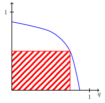
Figure 1: For fixed $\alpha$, say $\alpha=1/2$, we plot (in blue) the fraction $\eta$ of welfare from types above $c_{q}/\alpha=2c_{q}$ for $q\in[0,1]$. This curve is decreasing, and the intercept with the $y$-axis is typically smaller than $1$ because of the division of $c_{q}$ by $\alpha$. The best approximation guarantee that can be obtained with a given $\alpha$ is proportional to the area $\eta q$ of the largest box that fits under the curve (red, dotted). The larger this area the further away the setting from being point mass-like, and the better the approximation.

We provide a visual interpretation of the approximation guarantee from Theorem 1 in Figure 1. Intuitively, the conditions in Theorem 1 ensure that the welfare contribution from low types, i.e., types below $\frac{c_{q}}{\alpha}$, is sufficiently small compared to the optimal welfare. It is important to note that in order to guarantee constant approximations of linear contracts, it is sufficient to assume that the welfare is not concentrated around low types. This is because the welfare contribution is monotone in the agent’s cost in our model, ruling out the possibility of concentration on high types directly.

The proof of Theorem 1 utilizes a novel concept of being slowly-increasing (Definition 5), which can be applied to any cumulative distribution function and captures its rate of increase. In Theorem 2 below we provide a parametric approximation factor for linear contracts that depends on this rate of increase when the small-tail assumption is satisfied. Theorem 1 follows immediately from Theorem 2 by observing that any distribution is slowly-increasing for some parameters.

3.1 Approximation for Slowly-Increasing Distributions

Any distribution $G$ is an increasing function, and Definition 5 captures the rate of growth for function $G$. Namely, if the cost increases by a factor of $\frac{1}{\alpha}$ from $\alpha c$ to $c$, then the CDF should increase by a multiplicative factor of at most $\frac{1}{\beta}$ (i.e., $G(c)\leq\frac{1}{\beta}G(\alpha c)$). This condition becomes stronger the lower $\alpha$ is and the closer $\beta$ is to 1, and accordingly the approximation factor in the following theorem becomes better. Note that we require the condition to hold only for types above $\kappa$ for some parameter $\kappa\in[\underline{c},\bar{c}]$, that is, only for types that are not in the tail.

Definition 5 (Slowly-increasing distribution).

Let $\alpha,\beta\in(0,1]$ and $\kappa\in[\underline{c},\bar{c}]$. A distribution $G$ with support $[\underline{c},\,\overline{c}]$ is $(\alpha,\beta,\kappa)$-slowly-increasing if

$$G(\alpha c)\geq\beta G(c) \forall c\geq\kappa.$$

Intuitively, the slowly-increasing definition captures the spread of the type distribution. When the cumulative distribution function increases more slowly, the distribution is spread out over a wider range. With this property, linear contracts can generate revenue from low-cost types that approximately covers the welfare contribution from high-cost types. Additionally, the welfare contribution from a small range of low-cost types is not significant due to the small-tail assumption. The proof of Theorem 2 is provided in Section B.1.

Theorem 2.

Fix $\alpha,\beta,\eta\in(0,1]$. For any principal-agent instance, if there exists $\kappa\in[\frac{\underline{c}}{\alpha},\bar{c}]$ such that the instance has $(\alpha,\beta,\kappa)$-slowly-increasing distribution of agent types and satisfies the $(\kappa,\eta)$-small-tail for cost assumption, a linear contract with parameter $\alpha$ achieves expected revenue that is a $\frac{1}{(1-\alpha)\beta\eta}$-approximation to the optimal expected welfare.

Next we prove Theorem 1 by applying Theorem 2.

Proof of Theorem 1.

For any $q>0$ and any $\alpha\in(0,1)$, let $\kappa$ be the constant such that $G(\alpha\kappa)=q$. Note that by construction we have $\kappa\geq\frac{\underline{c}}{\alpha}$. For any distribution $G$ and any cost $c\geq\kappa$, we have

$$G(\alpha c)\geq G(\alpha\kappa)\geq G(\alpha\kappa)\cdot G(c)$$

where the last inequality holds since $G(c)\leq 1$ for any $c$. Therefore, distribution $G$ satisfies $(\alpha,G(\alpha\kappa),\kappa)$-slow-increasing condition. Under the additional assumption of $(\kappa,\eta)$-small-tail for cost, by applying Theorem 2, the approximation ratio of linear contracts to optimal welfare is

$$\frac{1}{\eta(1-\alpha)G(\alpha\kappa)}=\frac{1}{(1-\alpha)\eta q}$$

and Theorem 1 holds. ∎

Moreover, Theorem 2 allows us to obtain more refined approximation guarantees for broader classes of type distributions, e.g., distributions with non-increasing densities, which include uniform distributions and exponential distributions as special cases. The proof of Corollary 3 is provided in Section B.3.

Corollary 3.

For any principal-agent setting, if the type distribution has non-increasing density on $[\underline{c},\infty)$ with $\underline{c}\geq 0$, then $(\frac{\kappa+1}{2\kappa},\frac{1}{2},\kappa\underline{c})$-slowly-increasing is satisfied for any $\kappa>1$. With the assumption of $(\kappa\underline{c},\eta)$-small-tail, a linear contract achieves as revenue a $\frac{4\kappa}{\eta(\kappa-1)}$-approximation to the optimal welfare.

For example, when the principal-agent instance satisfies the $(3\underline{c},\frac{2}{3})$-small-tail assumption, i.e., the welfare contribution from types at most triple of the lowest type does not exceed one third of the optimal welfare, the revenue of the optimal linear contract is at least $\frac{1}{9}$ of the optimal welfare if the type distribution has non-increasing density. Moreover, in the special case of $\underline{c}=0$, the assumption of $(0,1)$-small-tail is satisfied for all distributions. Therefore, a linear contract achieves a $4$-approximation to the optimal welfare for distributions with non-increasing densities supported on $[0,\infty)$. The example with $\underline{c}=0$ is special because even if the types are concentrated around low values, the principal can incentivize the agent to exert high effort with almost zero payments, leading to revenue close to the optimal welfare.

Note that the approximation ratio of $4$ or $9$ in these examples may appear large at first glance. However, the benchmark here is the optimal welfare, which might be significantly higher than the optimal revenue, and hence the actual loss compared to the optimal revenue might be smaller. In fact, in Section 3.2 we provide an improved approximation ratio for distributions with non-increasing densities when compared to the optimal revenue under a slightly different small-tail assumption.

Moreover, the interpretation of the approximation result is not to take the constant factor too literally (Roughgarden and Talgam-Cohen,, 2019). Instead, we should focus on the relative comparison of the approximation factors in different environments. In our model, the worst-case approximation ratio with degenerate type distributions degrades linearly with the number of actions available to the agent, while the worst-case approximation ratio with sufficient uncertainty remains constant regardless of the number of actions. This illustrates that sufficient uncertainty is the main factor driving the approximate optimality of linear contracts in our Bayesian model.

3.2 Approximations for Linearly-Bounded Distributions

We next provide improved approximation guarantees with respect to the optimal revenue. Our distributional condition for this result captures how well the virtual cost is approximated by a linear function. We show that “the more linear” the virtual cost, the better a linear contract approximates the optimal expected virtual welfare (and hence the optimal revenue). This is formalized in Definition 6, where the ironed virtual cost of the distribution is sandwiched between two parameterized linear functions of the cost.

Definition 6 (Linearly-bounded distribution).

Let $\beta\leq\alpha\in(0,1]$. A distribution $G$ with support $[\underline{c},\bar{c}]$ satisfies $(\alpha,\beta,\kappa)$-linear boundedness if the corresponding ironed virtual value function satisfies

$$\frac{1}{\alpha}c\leq\bar{\varphi}(c)\leq\frac{1}{\beta}c \forall c\geq\kappa,$$

where $\kappa\in[\underline{c},\bar{c}].$

As pointed out by Bulow and Roberts, (1989), the ironed virtual value function $\bar{\varphi}(c)$ can be interpreted as the marginal cost function for incentivizing agent with type $c$ to choose the desirable action. Our assumption of linear boundedness holds if the marginal cost function has bounded rate of change.

To compare with the optimal revenue, our assumption of small-tail is defined on the virtual welfare instead of welfare, which is more suitable for quantifying the optimal revenue for a given contract instance. Let ${\rm VWel}_{[a,b]}\triangleq\int_{a}^{b}R_{i^{*}(r,\bar{\varphi}(c))}-\gamma_{i^{*}(r,\bar{\varphi}(c))}c\,{\rm d}c$ be the expected virtual welfare from types within $[a,b]$.

Definition 7 (Small-tail assumption for virtual welfare).

A principal-agent instance with types supported on $[\underline{c},\,\overline{c}]$ is $(\kappa,\eta)$-small-tail for virtual welfare if

$${\rm VWel}_{[\kappa,\,\overline{c}]}\geq\eta\cdot{\rm VWel}_{[\underline{c},\,\overline{c}]}.$$

Theorem 3.

Fix $\alpha,\beta,\eta\in(0,1]$. For any principal-agent instance and $\kappa$ such that the instance has $(\alpha,\beta,\kappa)$-linear bounded distribution of agent types and satisfies the $(\kappa,\eta)$-small-tail for virtual welfare assumption, the linear contract with parameter $\alpha$ achieves expected revenue that is:

1. a $\frac{1}{\eta(1-\alpha)}$-approximation to the optimal expected virtual welfare.

2. a $\frac{1-\beta}{\eta(1-\alpha)}$-approximation to the optimal expected virtual welfare if $i^{*}(r,\bar{\varphi}(\bar{c}))=0$.

The additional condition $i^{*}(r,\bar{\varphi}(\bar{c}))=0$ in Theorem 3.2 assumes that the highest cost type is sufficiently large such that the principal cannot incentivize this type to exert costly effort. This further ensures that the range of support for the cost distribution is sufficiently large and hence the approximation guarantee is improved.

We provide the detailed proof of Theorem 3.1 to illustrate the main ideas. The proof of Theorem 3.2 with refined approximations is provided in Section B.2.

Proof of Theorem 3.1.

Denote by ${\rm VWel}$ the optimal expected virtual welfare, and by ${\rm APX}$ the expected revenue of a linear contract with parameter $\alpha$; our goal is to show that ${\rm APX}\geq\eta(1-\alpha){\rm VWel}$. Recall $r$ represents the vector of rewards given different actions. Let $i^{*}(\alpha r,c)$ be the action that agent with type $c$ chooses given a linear contract with parameter $\alpha$, and let $i^{*}(r,\bar{\varphi}(c))$ be the virtual welfare maximizing action for agent with type $c$. We first show that under $(\alpha,\beta,\kappa)$-linear bounded assumption,

$$i^{*}(\alpha r,c)\geq i^{*}(r,\bar{\varphi}(c)),\quad\forall c\geq\kappa.$$

To do so, denote by $\hat{i}=i^{*}(r,\bar{\varphi}(c))$, we will first show that $\alpha R_{\hat{i}}-\gamma_{\hat{i}}c\geq\alpha R_{\ell}-\gamma_{\ell}c$ for any $\ell\leq\hat{i}$. Note that by the definition of $\hat{i}$, since $\ell$ is a feasible action choice, we have that $R_{\hat{i}}-\gamma_{\hat{i}}\bar{\varphi}(c)\geq R_{\ell}-\gamma_{\ell}\bar{\varphi}(c)$. That is, $R_{\hat{i}}-R_{\ell}\geq(\gamma_{\hat{i}}-\gamma_{\ell})\bar{\varphi}(c)$ for any $\ell\leq\hat{i}$. Combining the above with $\bar{\varphi}(c)\geq\frac{1}{\alpha}c$ for any $c\geq\kappa,$ we have $\alpha R_{\hat{i}}-\alpha R_{\ell}\geq(\gamma_{\hat{i}}-\gamma_{\ell})c$ for any $\ell\leq\hat{i}$ and any $c\geq\kappa$. Therefore, $\alpha R_{\hat{i}}-\gamma_{\hat{i}}c\geq\alpha R_{\ell}-\gamma_{\ell}c$ for any $\ell\leq\hat{i}$ and $c\geq\kappa$. This implies that $i^{*}(\alpha r,c)\geq\hat{i}=i^{*}(r,\bar{\varphi}(c))$ for any $c\geq\kappa$. Since the expected reward is monotone in the chosen action, we have

$$R_{i^{*}(\alpha r,c)}\geq R_{i^{*}(r,\bar{\varphi}(c))},\quad\forall c\geq\kappa.$$

We now use this to lower bound ${\rm APX}$. Recall that ${\rm APX}=\int_{\underline{c}}^{\bar{c}}g(c)(1-\alpha)R_{i^{*}(\alpha r,c)}\,{\rm d}c$. Since $R_{i}\geq 0$ $\forall i\in[n]$, ${\rm APX}\geq\int_{\kappa}^{\bar{c}}g(c)(1-\alpha)R_{i^{*}(\alpha r,c)}\,{\rm d}c$. By the above arguments we have that

$${\rm APX}\geq(1-\alpha)\int_{\kappa}^{\bar{c}}g(c)R_{i^{*}(r,\bar{\varphi}(c))}\,{\rm d}c.$$ (5)

Recall that ${\rm VWel}_{[\kappa,\bar{c}]}=\int_{\kappa}^{\bar{c}}g(c)(R_{i^{*}(r,\bar{\varphi}(c))}-\gamma_{i^{*}(r,\bar{\varphi}(c))}\bar{\varphi}(c))\,{\rm d}c$. Since $\gamma_{i}\geq 0$ for any $i\in[n]$ and $\bar{\varphi}(c)\geq 0$ for any $c\in[\underline{c},\bar{c}]$, the latter is bounded from above as $\int_{\kappa}^{\bar{c}}g(c)R_{i^{*}(r,\bar{\varphi}(c))}\,{\rm d}c$. Combining this with Equation 5, we have that

$${\rm APX}\geq(1-\alpha){\rm VWel}_{[\kappa,\bar{c}]}\geq\eta(1-\alpha){\rm VWel}.\qed$$

By Theorem 3 we obtain improved approximation ratios for several families of commonly observed distributions when compared to the optimal revenue, with proofs provided in Section B.3.

Corollary 4.

For any principal-agent setting, the following holds:

1. If the type distribution has non-increasing density on $[\underline{c},\infty)$ for $\underline{c}>0$, then $(\frac{\kappa}{2\kappa-1},0,\kappa\underline{c})$-linear boundedness is satisfied for any $\kappa>1$. With the assumption of $(\kappa\underline{c},\eta)$-small-tail for virtual welfare, a linear contract achieves a $\frac{2\kappa-1}{\eta(\kappa-1)}$-approximation to the optimal revenue.

2. If the type distribution is uniform $U[0,\bar{c}]$, then $(\frac{1}{2},\frac{1}{2},0)$-linear boundedness and $(0,1)$-small-tail for virtual welfare are satisfied. A linear contract is revenue optimal when $i^{*}(r,\bar{\varphi}(\bar{c}))=0$.

3. If the type distribution is normal $\mathcal{N}(\mu,\sigma^{2})$ truncated at $c=0$ with $\sigma\geq\frac{5}{2\sqrt{2}}\mu$, then $(\frac{2}{3},0,0)$-linear boundedness and $(0,1)$-small-tail for virtual welfare are satisfied. A linear contract achieves a $3$-approximation to the optimal revenue.

Again, in the special case of $\underline{c}=0$, the assumption of $(0,1)$-small-tail for virtual welfare is satisfied for all distributions. Therefore, a linear contract achieves a $2$-approximation to the optimal revenue for distributions with non-increasing densities supported on $[0,\infty)$. This improves the worst case approximation of $4$ when compared to the optimal welfare. Moreover, our method allows us to establish the exact optimality of linear contracts for uniform distribution when the types are sufficiently dispersed, i.e., when $i^{*}(r,\bar{\varphi}(\bar{c}))=0$. We also obtain constant approximation bounds for truncated normal distributions when the variance is large, a commonly adopted metric for measuring the amount of uncertainty in type distributions.

Gottlieb and Moreira, (2022) give a condition under which debt contracts are optimal. This is not in contrast to our result establishing the optimality of linear contracts for uniform distributions, because their result requires there to be a zero cost action that leads to positive reward (see Footnote 8 of their paper), which is not the case in our model.

3.3 Tight Approximation for General Distributions

We present a tight $\Theta(n)$-approximation guarantee for linear contracts for general distributions without small-tail assumptions. The lower bound of $\Omega(n)$ is already illustrated in Example 1 for uniform type distributions, and our upper bound provides a tight approximation guarantee for any type distribution. Our bounds imply that a linear contract achieves a constant approximation to the optimal revenue when the number of actions is a constant. This is in sharp contrast to the multi-dimensional type model of Guruganesh et al., (2021) and Castiglioni et al., (2021), where the approximation ratio is unbounded even for a constant number of actions.

Theorem 4.

For any principal-agent instance with $n$ actions, a linear contract achieves expected revenue that is an $n$-approximation to the optimal revenue.

The proofs appear in Appendix B.5. The proof of Theorem 4 relies on similar insights on the sets of breakpoints as in the proof of Theorem 3.

4 Undesirable Properties of Optimal Contracts

We explore the properties of optimal contracts in our single-dimensional private types setting. We focus on deterministic contracts as introduced in Section 2.2. We first show that the optimal principal utility may exhibit unnatural non-monotonicity. Specifically, the optimal revenue of the principal may be strictly smaller when contracting with a stronger agent (in terms of lower cost per unit-of-effort). Secondly, we show that the amount of communication required to describe the optimal contract to the agent can be unbounded. These two properties make it less desirable to implement the optimal contract in practical situations.

4.1 Non-monotonicity of the Optimal Revenue

One way in which optimal contracts defy intuition is that a principal contracting with a stronger agent cannot necessarily expect higher revenue. Such non-monotonicity is known for auctions but only for multi-dimensional types (Hart and Reny,, 2015). To show this for contracts with single-dimensional types, we keep the contract setting fixed and consider two type distributions $G$ and $H$, where $H$ first-order stochastically dominates $G$. Formally, $H\succ_{\rm FOSD}G$ if $G(c)\geq H(c)$ $\forall c\in C$, that is, types drawn from $G$ are more likely to have lower cost than those drawn from $H$. One would expect that the principal’s revenue when agent costs are distributed according to $G$ would be higher, but this is not always the case — the proof relies on Example 2.

Proposition 1.

There exist a principal-agent setting and distributions $H\succ_{\rm FOSD}G$ such that the optimal expected revenue from an agent drawn from $G$ is smaller than an agent drawn from $H$.

Example 2.

Let $\delta,\epsilon\to 0$, and consider the following parameterized setting with $4$ actions and $4$ outcomes. The costs in units-of-effort per action are $\gamma_{0}=0,\gamma_{1}=0,\gamma_{2}=\frac{1}{2},\gamma_{3}=\frac{1}{\delta}$, and the rewards are $r_{0}=r_{1}=r_{2}=0$ and $r_{3}=\frac{1}{\delta}$. The distributions over outcomes per action are $F_{0}=(1,0,0,0)$, $F_{1}=(0,1-0.25\delta,0,0.25\delta)$, $F_{2}=(0,0.5-\delta,0.5,\delta)$, $F_{3}=(0,0,1-\delta-\delta^{2},\delta+\delta^{2})$. The type distributions $H\succ_{\rm FOSD}G$ are of the form:

$$G(c)=\begin{cases}\epsilon&c\in[0,1),\\ 1-\epsilon&c=1,\end{cases} H(c)=\begin{cases}0&c\in[0,1),\\ 1&c=1.\end{cases}$$

We outline the proof intuition here and defer the details to Appendix C.1. The three non-null actions have the following characteristics. Action $1$ requires no effort and generates small expected reward, action $2$ requires little effort and generates moderate reward, and action $3$ requires very high effort and generates slightly higher reward than action 2. Consider type $c=1$; incentivizing action $2$ is optimal for the principal. But the construction is such that incentivizing action $2$ can only be achieved via payment for outcome $2$, which in turn implies extremely large payment for action $3$. Unlike type $c=1$ who never takes action $3$ due to its high cost, type $c=0$ has the same zero cost for all actions. If the type distribution is such that $c=0$ can occur (i.e., $G$ rather than $H$), the principal will more often have to transfer this large payment (for outcome $2$) to the agent. There is thus a trade-off from having a low-cost type in the support, which ultimately leads to loss of revenue.

4.2 Menu-size Complexity

By the taxation principle, every IC contract has an equivalent non-direct-revelation representation, which offers the agent a menu of payment profiles (rather than asking the agent to reveal his type then presenting him with a payment profile). Given a menu of payment profiles, the agent will choose a payment profile from the menu and an action to maximize his expected utility based on his private type.

In this section we adapt the measure of menu-size complexity suggested for auctions by Hart and Nisan, (2019), to our context of contracts with private types. Formally, the menu-size complexity of a contract design instance is the number of different payment profiles offered in the menu representation.

Definition 8.

The menu-size complexity of a payment rule $t:C\to\mathbb{R}^{m}$ is the image size of function $t$.

The menu-size complexity captures the amount of information transferred from the principal to the agent in a straightforward communication of the contract. In auctions it has been formally tied to communication complexity Babaioff et al., (2017). Intuitively, a contract with larger menu-size complexity requires more complex communication to describe the contract to the agent, and hence harder to be implemented in practice. We show that even with constant number of possible outcomes, the menu-size complexity of the optimal contract can be arbitrarily large. In contract, linear contracts have menu-size complexity of 1. The proof of the following proposition is provided in Section C.2.

Proposition 2.

For every $n>1$ there exists a principal-agent setting with $m=2$ outcomes such that the menu-size complexity of the optimal contract is at least $\frac{n-1}{2}$.

Appendix A Characterization of IC Contracts

This appendix complements Section 2.3. We present the details for the proof of Lemma 1 in Section A.1. For completeness and comparison, we also present the dual characterization from Alon et al., (2021) in Section A.2.

A.1 Primal Characterization

In this section we complete the proof of Lemma 1 from Section 2.3. The proof relies on the Envelope Theorem as follows.

Lemma 2 (The Envelope Theorem (Milgrom and Segal,, 2002)).

Consider the problem of choosing $b$ to maximize a function $f(b;a)$, where $a$ is a parameter. Denote the solution to this maximization by $b(a)$ and define the maximum value function $V(a)$ by $V(a)=max_{b}f(b;a)=f(b(a);a)$. The derivative of the value function is the partial derivative of the objective evaluated at the solution to the optimization.

$$\frac{dV(a)}{da}=\frac{\,{\rm d}f(b;a)}{\,{\rm d}a}\mid_{b=b(a)}$$

Before the proof of Lemma 1, we illustrate the intuition behind integral monotonicity. In classic mechanism design settings, any option from the truthful mechanism — when viewed as a menu of (allocation, payment) pairs — induces a utility function linear in the agent’s type. Hence, the agent’s interim utility (i.e., his utility knowing his own type) is the maximum over linear functions. In contrast, in our setting any option from the IC contract — when viewed as a menu of payment vectors — induces a choice for the agent. The agent chooses the action that maximizes his utility given his private cost. Hence the induced utility function is the maximum over linear functions in the agent’s type, i.e., a convex function. The agent’s interim utility is thus the maximum over convex functions. This difference between “max-over-linear” and “max-over-convex” is the main driving force that makes contract design with types a complicated problem. While max-over-convex does imply that the agent’s interim utility is convex and the allocation rule necessarily monotone, these conditions are no longer sufficient for truthful implementation. We need to impose additional constraints on the curvature of the interim utility, so that it can be represented as the maximum over a set of “feasible” convex functions.

Proof of Lemma 1.

Let $u(c)$ be agent’s utility for following the mechanism and let $u_{c}(z)$ be the utility function of the agent with type $z$ when he has reported $c$ to the principal. By the Envelope Theorem (Lemma 2) $u^{\prime}_{c}(z)=-\gamma_{i^{*}(t^{c},z)}$, and since $u^{\prime}(c)=-\gamma_{x(c)}$, we have that for any $c,c^{\prime}$,

$$u(c^{\prime}) =u(c)-\int_{c}^{c^{\prime}}\gamma_{x(z)}\,{\rm d}z$$

and

$$u_{c}(c^{\prime}) =u_{c}(c)-\int_{c}^{c^{\prime}}\gamma_{i^{*}(t^{c},z)}\,{\rm d}z.$$

Note that the agent with cost $c^{\prime}$ has no incentive to deviate the report to $c$ if and only $u(c^{\prime})\geq u_{c}(c^{\prime})$, which is equivalent to

$$\int_{c}^{c^{\prime}}\gamma_{x(z)}-\gamma_{i^{*}(t^{c},z)}\,{\rm d}z\leq 0,\qquad\forall c^{\prime}$$

since $u_{c}(c)=u(c)$. Now given any implementable allocation rule $x$, the corresponding interim utility satisfies $u(c)=u(\bar{c})+\int_{c}^{\bar{c}}\gamma_{x(z)}\,{\rm d}z$ and hence

$$T^{c}_{x(c)} =\gamma_{x(c)}\cdot c+u(\bar{c})+\int_{c}^{\bar{c}}\gamma_{x(z)}\,{\rm d}z$$

$$=\gamma_{x(c)}\cdot c+\int_{c}^{\bar{c}}\gamma_{x(z)}\,{\rm d}z+(T^{\bar{c}}_{x(\bar{c})}-\bar{c}\cdot\gamma_{x(\bar{c})}).\qed$$

A.2 Dual Characterization

For completeness, we present here a dual characterization for implementable allocation rules due to Alon et al., (2021). In this section, we will focus on the allocation for deterministic contracts. As established in previous subsection, every such implementable allocation rule is monotone, and in particular monotone piecewise constant (see Definition 9). The characterization is obtained via a discretization of the type space to the set of allocation rule’s breakpoints and applying an LP-duality approach for characterizing implementable discrete allocation rules.

Note that the indexing here is slightly different than the indexing in Definition 9 for consistency.

Lemma 3 (Theorem 3.8 in Alon et al., (2021)).

An allocation rule $x:\mathbb{R}\rightarrow[n]$ is implementable if and only if it is monotone piecewise constant with breakpoints $0=z_{0}<...<z_{\ell+1}=\bar{c}$ and there exist no weights $\lambda_{(R,i,{i^{\prime}},k)},\lambda_{(L,i+1,{i^{\prime}},k)}\geq 0,$ for all $i\in[\ell],i^{\prime}\in[\ell+1],k\in[n]$ which satisfy $\sum_{i^{\prime},k\in[n]}\lambda_{(L,i+1,i^{\prime},k)}=\sum_{i^{\prime},k\in[n]}\lambda_{(R,i,i^{\prime},k)}=1$ $\forall i\in[\ell]$ and the following conditions:

1. Weakly dominant distributions:

   $$\sum_{i^{\prime}\in[\ell],k\in[n]}\frac{1}{2}(\lambda_{(R,i^{\prime},i,k)}F_{k,j}+\lambda_{(L,i^{\prime}+1,i,k)}F_{k,j})\geq F_{x(z_{i}),j} \forall j\in[m],i\in[\ell].$$

2. Strictly lower joint cost:

   $$\sum_{i\in[\ell]}(\gamma_{x(z_{i})}z_{i}+\gamma_{x(z_{i})}z_{i+1})>\sum_{i\in[\ell],i^{\prime}\in[\ell+1],k\in[n]}\lambda_{(R,i,i^{\prime},k)}\gamma_{k}z_{i}+\lambda_{(L,i+1,i^{\prime},k)}\gamma_{k}z_{i+1}.$$

Recall definition 9 of piecewise constant monotone allocation rules. The key observation for this result is that ensuring IC for both endpoints of an interval $[z_{i},z_{i+1})$ suffices to guarantee IC for all types in the interval as well. This forms a natural continuous-to-discrete reduction. Since each breakpoint $z_{i}$ serves as an endpoint of two distinct intervals (from $z_{i}^{+}$ and $z_{i}^{-}$), two copies of the breakpoint are involved, referred to as $R$ and $L$ for right and left respectively.

The conditions for ensuring IC on this discrete set of types can be explained as follows. One can think of the weights $\lambda$ as a deviation plan, by which whenever the true type is (w.l.o.g) $z_{i}^{+}$ then with probability $\lambda_{(R,i,i^{\prime},k)}$ he deviates to type $z_{i^{\prime}}$ and to action $k$ (i.e., he pretends to be of type $z_{i^{\prime}}$ and takes action $k$). This theorem states that an allocation rule is implementable precisely when there is no deviation plan from the principal’s recommendation which costs strictly less for the agents, and enables them to dominate the distribution over outcomes resulted by the principal’s recommendation. It can be verified that in a setting without moral hazard, this can happen only when the allocation rule is not monotone.

A.3 Monotone Virtual Welfare Maximization is not Sufficient

Given Corollary 2, one may be tempted to optimize revenue by maximizing virtual welfare. Indeed one of the most appealing results of Myerson, (1981) is that optimizing revenue can be reduced to maximizing virtual welfare. In this section we show that virtual welfare maximization can be unimplementable when moral hazard is involved. The proof relies on Example 3, showing there exists no payment scheme for this allocation rule that satisfies the curvature constraints of Lemma 1.

Proposition 3.

The virtual welfare maximizing allocation rule $x^{*}$ is not always implementable, even when monotone.

Example 3.

Consider the following setting with $4$ actions and $3$ outcomes. The costs in units-of-effort per action are $\gamma_{0}=0,\gamma_{1}=1,\gamma_{2}=3,\gamma_{3}=5.5$, and the rewards are $r_{0}=0,r_{1}=100,r_{2}=300$. The distributions over outcomes per action are $F_{0}=(1,0,0)$, $F_{1}=(0,1,0)$, $F_{2}=(0,0.5,0.5)$, $F_{3}=(0,0,1)$. The type set is $C=[0,10]$. Taking $\delta=\frac{20}{23}$, the type distribution over $C$ is as follows.

$$g(c)=\begin{cases}\delta&c\in[0,1],\\ 0.025\delta&c\in(1,4],\\ 0.0125\delta&c\in(4,10],\end{cases} G(c)=\begin{cases}\delta c&c\in[0,1],\\ 0.025\delta(c-1)+\delta&c\in(1,4],\\ 0.0125\delta(c-4)+1.075\delta&c\in(4,10].\end{cases}$$

Before proving Proposition 3 we establish the following claim.

Claim 1.

Consider Example 3. The virtual welfare maximizing allocation rule is given by

$$x^{*}(c)=\arg\max_{i\in[n]}\{R_{i}-\gamma_{i}\varphi(c)\}=\begin{cases}3&c\in[0,1),\\ 2&c\in[1,4),\\ 1&c\in[4,9),\\ 0&c\in[9,10).\end{cases}$$

Proof.

The virtual cost $\varphi(c)=c+\frac{G(c)}{g(c)}$ is as follows:

$$\varphi(c)=\begin{cases}c+c&c\in[0,1),\\ c+c-1+\frac{1}{0.025}&c\in[1,4),\\ c+c-4+\frac{1.075}{0.0125}&c\in[4,10),\end{cases} =\begin{cases}2c&c\in[0,1),\\ 2c+39&c\in[1,4),\\ 2c+82&c\in[4,10).\end{cases}$$

The virtual welfare of every action is thus given by:

$$R_{3}-\gamma_{3}\varphi(c) = \begin{cases}300-11c&c\in[0,1),\\ -14.5-11c&c\in[1,4),\\ -151-11c&c\in[4,10),\end{cases}$$

$$R_{2}-\gamma_{2}\varphi(c) = \begin{cases}200-6c&c\in[0,1),\\ 83-6c&c\in[1,4),\\ -46-6c&c\in[4,10),\end{cases}$$

$$R_{1}-\gamma_{1}\varphi(c) = \begin{cases}100-2c&c\in[0,1),\\ 61-2c&c\in[1,4),\\ 18-2c&c\in[4,10),\end{cases}$$

and $R_{0}-\gamma_{0}\varphi(c)=0$. Therefore, the virtual welfare maximizing allocation rule is given by

$$x^{*}(c)=\arg\max_{i\in[n]}\{R_{i}-\gamma_{i}\varphi(c)\}=\begin{cases}3&c\in[0,1),\\ 2&c\in[1,4),\\ 1&c\in[4,9),\\ 0&c\in[9,10),\end{cases}$$

as claimed. ∎

Proof of Proposition 3.

The unique virtual welfare maximizing allocation rule $x^{*}$ in Example 3 assigns action $3$ for $c\in[0,1]$, action $2$ for $c\in(1,4]$, action $1$ for $c\in(4,9]$, and action $0$ for $c\in(9,10]$ (see 1). This allocation rule is monotone and can be verified using the definitions of virtual cost $\varphi(c)=c+G(c)/g(c)$ and virtual welfare $R_{i}-\gamma_{i}\varphi(c)$. By Equation 2 of Lemma 1, to establish that this rule is not implementable it suffices to show the following: For type $c=4$ and every payment scheme $t^{4}\in\mathbb{R}^{m+1}$ that satisfies $x^{*}(4)=i^{*}(t^{4},4)$, it holds that $\int_{4}^{1}\gamma_{x(z)}-\gamma_{i^{*}(t^{4},z)}\,{\rm d}z>0$. I.e., any candidate payment scheme $t^{4}$ must violate integral monotonicity, completing the proof.

To establish this, note that since $x^{*}(4)=i^{*}(t^{4},4)$, action $x^{*}(4)=2$ gives higher utility for type $c=4$ than the utility from action $1$. This implies that $0.5({t^{4}_{1}+t_{2}^{4}})-12\geq t^{4}_{1}-4$. That is, $t^{4}_{2}-t^{4}_{1}\geq 16.$ In this case, it can be verified that for types $c\leq c^{\prime}$ where $c^{\prime}$ is at least $3.2$ (the exact value of $c^{\prime}$ depends on the precise payment scheme $t^{4}$), the utility from $t^{4}$ is maximized when taking action $3$, i.e, $i^{*}(t^{4},c)=3$. Further, $i^{*}(t^{4},c)=2$ for $[c^{\prime},4]$. We thus have that $\int^{1}_{4}\gamma_{x^{*}(z)}-\gamma_{i^{*}(t^{4},z)}\,{\rm d}z$ is equal to $\int^{c^{\prime}}_{1}\gamma_{3}-\gamma_{2}\,{\rm d}z+\int^{4}_{c^{\prime}}\gamma_{2}-\gamma_{2}\,{\rm d}z$, which is strictly positive. ∎

We end this section by showing that the trouble in Example 3 stems from the agent’s ability to double-deviate — to both an untruthful type and an unrecommended action. In particular we show that types $c=1$ and $c=4-\epsilon\to 4$ cannot be jointly incentivized by any contract to take action $2$. Suppose towards a contradiction that there exist such payment schemes $t^{1}=(t^{1}_{0},t^{1}_{1},t^{1}_{2})$ and $t^{4}=(t_{0}^{4},t_{1}^{4},t_{2}^{4})$ for types $c=1$ and $c=4-\epsilon$, respectively. By IC, the expected payment for action $2$ in both contracts is equal (otherwise both agents prefer one of these payment profiles). That is, $0.5(t^{1}_{2}+t^{1}_{1})=0.5(t^{4}_{2}+t^{4}_{1})$. Let us assume w.l.o.g. that $t^{1}_{2}-t^{1}_{1}\geq t^{4}_{2}-t^{4}_{1}$. By IC, an agent of type $c=4$ is better off by reporting truthfully and taking action $2$, over taking action $1$. Therefore, $0.5({t^{4}_{1}+t_{2}^{4}})-12\geq t^{4}_{1}-4$. That is, $t^{4}_{2}-t^{4}_{1}\geq 16.$ Similarly, the agent of type $c=1$, is better off by reporting truthfully, and taking action $2$, over taking action $3$. This implies that $0.5(t^{1}_{1}+t^{1}_{2})-3\geq t^{1}_{2}-5.5$. That is, $t^{1}_{2}-t^{1}_{1}\leq 5$. This implies that $5\geq t^{1}_{2}-t^{1}_{1}\geq t^{4}_{2}-t^{4}_{1}\geq 16$, a contradiction.

Appendix B Near-Optimality of Linear Contracts

In this section we provide the proofs (or the parts of the proofs) omitted from Section 3 on the near-optimality of linear contracts.

B.1 Slowly-Increasing Distributions

Proof of Theorem 2.

Denote by ${\rm Wel}$ the optimal expected welfare, and by ${\rm APX}$ the expected revenue of a linear contract with parameter $\alpha$; we show that ${\rm APX}\geq(1-\alpha)\beta\eta\cdot{\rm Wel}$.

Recall the notion of $i^{*}(t^{\hat{c}},c)$ above. Note that replacing $t^{\hat{c}}$ with $r$ implies transferring the entire reward to the agent, so $i^{*}(r,c)$ is the welfare maximizing action for type $c$. Then the welfare from types above $\kappa$ is

$${\rm Wel}_{[\kappa,\,\bar{c}]} =\int_{\kappa}^{\infty}g(c)(R_{i^{*}(r,c)}-\gamma_{i^{*}(r,c)}\cdot c)\,{\rm d}c$$

$$=-G(\kappa)\cdot(R_{i^{*}(r,\kappa)}-\gamma_{i^{*}(r,\kappa)}\cdot\kappa)+\int_{\kappa}^{\infty}G(c)\gamma_{i^{*}(r,c)}\,{\rm d}c,$$

where the equality holds by integration by parts and the fact that the derivative of $R_{i^{*}(r,c)}-\gamma_{i^{*}(r,c)}c$ with respect to $c$ is $-\gamma_{i^{*}(r,c)}$ (cf., Lemma 2). Further, note that

$$i^{*}(\alpha r,c)=\arg\max_{i\in[n]}\alpha R_{i}-\gamma_{i}c=\alpha\arg\max_{i\in[n]}R_{i}-\gamma_{i}\frac{c}{\alpha}=i^{*}(r,\frac{c}{\alpha})$$

Therefore, the revenue of ${\rm APX}$ is

$${\rm APX}=\int_{\underline{c}}^{\infty}(1-\alpha)R_{i^{*}(r,\frac{c}{\alpha})}g(c)\,{\rm d}c\geq(1-\alpha)\int_{\underline{c}}^{\infty}g(c)(R_{i^{*}(r,\frac{c}{\alpha})}-\gamma_{i^{*}(r,\frac{c}{\alpha})}\alpha c))\,{\rm d}c,$$ (6)

where the inequality holds simply because $\gamma_{i^{*}(r,\frac{c}{\alpha})}\cdot\alpha c$ is non-negative. Using integration by parts:

$${\rm APX} \geq(1-\alpha)\alpha\int_{\underline{c}}^{\infty}G(c)\gamma_{i^{*}{(r,\frac{c}{\alpha})}}\,{\rm d}c$$

$$=(1-\alpha)\int_{\frac{\underline{c}}{\alpha}}^{\infty}G(\alpha c)\gamma_{i^{*}({r,c})}\,{\rm d}c\geq(1-\alpha)\int_{\kappa}^{\infty}G(\alpha c)\gamma_{i^{*}({r,c})}\,{\rm d}c.$$

Since $G(\alpha c)\geq\beta G(c)$ for any $c\geq\kappa$, we have that

$${\rm APX}\geq(1-\alpha)\beta\cdot{\rm Wel}_{[\kappa,\,\bar{c}]}\geq(1-\alpha)\beta\eta\cdot{\rm Wel},$$

where the last inequality holds by $(\kappa,\eta)$-small-tail assumption. ∎

B.2 Linearly-Bounded Distributions

Our proof of Theorem 3.2 relies on the characterization of monotone piecewise constant allocation rules in IC contracts. Note that a necessary property of the allocation rule that ensures IC is monotonicity. In our context, a monotone allocation rule recommends actions that are more costly in terms of effort — and hence more rewarding in expectation for the principal — to agents whose cost per unit-of-effort is lower. Intuitively, such agents are better-suited to take on effort-intensive tasks. Since the number of actions is finite, the class of monotone allocation rules boils down to the class of monotone piecewise constant rules. Informally, these are rules such that: (i) the allocation function $x(\cdot)$ is locally constant in distinct intervals within $[0,\bar{c}]$; and (ii) the allocation is decreasing with intervals. Formally:

Definition 9.

An allocation rule $x:C\to[n]$ is monotone piecewise constant if there exist $\ell+2$ breakpoints $\underline{c}=z_{\ell+1}<...<z_{0}=\bar{c}$ where $\ell\leq n$, such that $\forall i\in[\ell]$:

1. $c\in(z_{i+1},z_{i}]\implies x(c)=x(z_{i})$;

2. $x(z_{i+1})>x(z_{i})$.

Proof of Theorem 3.2.

Assume that $i^{*}(r,\bar{\varphi}(\bar{c}))=0$, and denote by ${\rm VWel}$ the optimal expected virtual welfare, and by ${\rm APX}$ the expected revenue of a linear contract with parameter $\alpha$; our goal is to show that ${\rm APX}\geq\frac{\eta(1-\alpha)}{1-\beta}{\rm VWel}$. Let $x_{{\rm Wel}}$ be the welfare maximizing allocation rule, $x_{{\rm VWel}}$ be the virtual welfare maximizing allocation rule, and let $x_{{\rm APX}}$ be the allocation rule induced by a linear contract with parameter $\alpha$. That is, $\forall c\in C$

$$x_{{\rm Wel}}(c) = \arg\max_{i\in[n]}\{R_{i}-\gamma_{i}c\},$$

$$x_{{\rm VWel}}(c) = \arg\max_{i\in[n]}\{R_{i}-\gamma_{i}\bar{\varphi}(c)\},$$ (7)

$$x_{{\rm APX}}(c) = \arg\max_{i\in[n]}\{\alpha R_{i}-\gamma_{i}c\}.$$

Denote the breakpoints (as defined in Definition 9) of $x_{{\rm Wel}},x_{{\rm VWel}}$ and $x_{{\rm APX}}$ by $\{z_{{\rm Wel},i}\}$, $\{z_{{\rm VWel},i}\}$, and $\{z_{{\rm APX},i}\}$ respectively. Let $|\{z_{{\rm Wel},i}\}|$ be the image size of $x_{{\rm Wel}}$. Throughout the proof we will assume that $n+2=|\{z_{{\rm Wel},i}\}|$, i.e., that all actions are allocated by $x_{{\rm Wel}}$. This is for ease of notation since in this case $x_{{\rm Wel}}(z_{{\rm Wel},i})=i$, but the same arguments apply when $|\{z_{{\rm Wel},i}\}|<n+2$. Since $\bar{\varphi}(c),\alpha c$ are increasing and $x_{{\rm Wel}}(\bar{c})=0$ since $i^{*}(r,\bar{\varphi}(\bar{c}))=0$, one can observe that $x_{{\rm VWel}},x_{{\rm Wel}}$ and $x_{{\rm APX}}$ have the same image size $n+2=|\{z_{{\rm VWel},i}\}|=|\{z_{{\rm APX},i}\}|$. Further, their breakpoints satisfy

$$\forall i\in[n+1]: z_{{\rm VWel},i}=\bar{\varphi}^{-1}(z_{{\rm Wel},i}), z_{{\rm APX},i}=\alpha z_{{\rm Wel},i}.$$ (8)

To see why the second part of (8) holds, consider for instance the breakpoint $z_{{\rm APX},n}$ (where $\alpha R_{n}-\gamma_{n}z_{{\rm APX},n}=\alpha R_{n-1}-\gamma_{n-1}z_{{\rm APX},n}$), and the breakpoint $z_{{\rm Wel},n}$ (where $R_{n}-\gamma_{n}z_{{\rm Wel},n}=R_{n-1}-\gamma_{n-1}z_{{\rm Wel},n}$). Note that by reorganizing the above, $z_{{\rm APX},n}$ can be rewritten as $\alpha(R_{n}-R_{n-1})/(\gamma_{n}-\gamma_{n-1})$. Similarly, $z_{{\rm Wel},n}$ can be rewritten as $(R_{n}-R_{n-1})/(\gamma_{n}-\gamma_{n-1})$.

We first aim to lower bound ${\rm APX}$. Note that the expected revenue for action $i\in[n]$ in a linear contract with parameter $\alpha$ is $(1-\alpha)R_{i}$. Further, recall that all types $c\in(z_{{\rm APX},i+1},z_{{\rm APX},i}]$ are allocated with the same action of $x_{{\rm APX}}(z_{{\rm APX},i})=i$. Thus, the expected revenue over all types can be phrased by the breakpoints as follows ${\rm APX}=\sum_{i\in[n]}(G(z_{{\rm APX},i})-G(z_{{\rm APX},i+1}))(1-\alpha)R_{i}$. By reorganizing the latter as shown in Claim 2 in Appendix B.2 we have

$${\rm APX} = \sum_{i\in[n-1]}G(z_{{\rm APX},i+1})(1-\alpha)(R_{i+1}-R_{i}).$$

Let $n-j=\min_{i\in[n+1]}\{z_{{\rm VWel},i}\mid\kappa\leq z_{{\rm VWel},i}\}$. In words, $z_{{\rm VWel},n-j}$ is the first breakpoint that is larger than $\kappa$. To lower bound ${\rm APX}$ we show that $G(z_{{{\rm APX}},i+1})\geq G(z_{{{\rm VWel}},i+1})$ $\forall i\in[n-j-1]$. Note that by (8), $z_{{{\rm APX}},i+1}=\alpha z_{{{\rm Wel}},i+1}$. Further, by the condition that $\frac{1}{\alpha}c\leq\bar{\varphi}(c)$ $\forall\kappa\leq c$, we have that $\bar{\varphi}^{-1}(c)\leq\alpha c$ $\forall\kappa\leq c$ (since both sides of the inequality are increasing). Therefore, $\bar{\varphi}^{-1}(z_{{{\rm Wel}},i+1})\leq\alpha z_{{{\rm Wel}},i+1}=z_{{{\rm APX}},i+1}$ $\forall i\in[n-j-1]$. Using (8) again for $z_{{{\rm VWel}},i+1}=\bar{\varphi}^{-1}(z_{{{\rm Wel}},i+1})$, we have that $z_{{{\rm VWel}},i+1}\leq z_{{{\rm APX}},i+1}$ $\forall i\in[n-j-1]$, which implies $G(z_{{{\rm VWel}},i+1})\leq G(z_{{{\rm APX}},i+1})$ $\forall i\in[n-j-1]$ as desired. Therefore, and since $R_{i+1}\geq R_{i}$ $\forall i\in[n-1]$ we have that

$${\rm APX}\geq\sum_{i\in[n-j-1]}G(z_{{\rm VWel},i+1})(1-\alpha)(R_{i+1}-R_{i}).$$ (9)

Next, we lower bound the right hand side of (9) using ${\rm VWel}_{[}\kappa,\bar{c}]$. First, we show in Claim 3 in Section B.2 that the optimal virtual welfare can also be phrased using the breakpoints as follows: ${\rm VWel}_{[\kappa,\bar{c}]}=\sum_{i\in[n-j-1]}G(z_{{\rm VWel},i+1})[R_{i+1}-R_{i}-z_{{\rm VWel},i+1}(\gamma_{i+1}-\gamma_{i})]-G(\kappa)(R_{n-j}-\gamma_{x(\kappa)}\kappa).$ Recall that by definition of $x_{{\rm VWel}}$, we have that $n-j\in\arg\max_{i\in[n]}\{R_{i}-\gamma_{i}\bar{\varphi}(\kappa)\}$. Therefore, $R_{i}-\gamma_{i}\bar{\varphi}(\kappa)\geq 0$. Which implies, since $\bar{\varphi}(\kappa)\geq\kappa$ that $R_{n-j}-\gamma_{x(\kappa)}\kappa\geq 0$. Thus,

$$\sum_{i\in[n-j-1]}G(z_{{\rm VWel},i+1})[R_{i+1}-R_{i}-z_{{\rm VWel},i+1}(\gamma_{i+1}-\gamma_{i})] \geq {\rm VWel}_{[\kappa,\bar{c}]}.$$ (10)

By Definition 9, the expected welfare at the breakpoint $z_{{\rm Wel},i+1}$ given actions $i+1$ and $i$ are equal. Thus, $R_{i+1}-R_{i}=(\gamma_{i+1}-\gamma_{i})z_{{\rm Wel},i+1},\forall i\in[n-1]$. Multiplying both sides by $\beta$ and using $\beta z_{{\rm Wel},i+1}\leq\bar{\varphi}^{-1}(z_{{\rm Wel},i+1})=z_{{\rm VWel},i+1}$ $\forall i\in[n-j-1]$, we have that $\beta(R_{i+1}-R_{i})\leq(\gamma_{i+1}-\gamma_{i})z_{{\rm VWel},i+1}$ $\forall i\in[n-j-1]$. Combining the latter with (10), we have that

$$\sum_{i\in[n-j-1]}G(z_{{\rm VWel},i+1})(1-\beta)(R_{i+1}-R_{i}) \geq {\rm VWel}_{[\kappa,\bar{c}]}.$$ (11)

Combining (9), (11) and the fact that ${\rm VWel}_{[\kappa,\bar{c}]}\geq\eta\cdot{\rm VWel}$, we have that ${\rm APX}\geq\frac{\eta(1-\alpha)}{1-\beta}{\rm VWel}$. ∎

The following claims completes the proof of Theorem 3.

Claim 2.

Consider ${\rm APX}$, and $z_{{\rm APX},i}$ $\forall i\in[n+1]$ as defined in the proof of Theorem 3.

$${\rm APX} = \sum_{i\in[n-1]}G(z_{{\rm APX},i+1})(1-\alpha)(R_{i+1}-R_{i}).$$

Proof.

As in the proof of Theorem 3

$${\rm APX}=\sum_{i\in[n]}(G(z_{{\rm APX},i})-G(z_{{\rm APX},i+1}))(1-\alpha)R_{i}.$$

Which, by splitting the sum is equal to

$$\sum_{i\in[n]}G(z_{{\rm APX},i})(1-\alpha)R_{i}-\sum_{i\in[n]}G(z_{{\rm APX},i+1})(1-\alpha)R_{i}.$$

Note that since $R_{0}=0$, the first term can be re-indexed as $\sum_{i\in[n-1]}G(z_{{\rm APX},i+1})(1-\alpha)R_{i+1}$. Further, since $G(z_{{\rm APX},n+1})=0$, we have that second term is equal to $\sum_{i\in[n-1]}G(z_{{\rm APX},i+1})(1-\alpha)R_{i}.$ Thus,

$${\rm APX}=\sum_{i\in[n-1]}G(z_{{\rm APX},i+1})(1-\alpha)(R_{i+1}-R_{i}).\qed$$

Claim 3.

Let $\kappa\in[\underline{c},\bar{c}]$, and consider $x_{\rm VWel}$, and $z_{{\rm VWel},i}$ for any $i\in[n+1]$ as defined in the proof of Theorem 3. The welfare contribution ${\rm VWel}_{[\kappa,\bar{c}]}$ equals

$$\sum_{i\in[n-j-1]}G(z_{{\rm VWel},i+1})[R_{i+1}-R_{i}-z_{{\rm VWel},i+1}(\gamma_{i+1}-\gamma_{i})]-G(\kappa)(R_{n-j}-\gamma_{x(\kappa)}\kappa),$$

where $n-j=\min_{i\in[n+1]}\{z_{{\rm VWel},i}\mid\kappa\leq z_{{\rm VWel},i}\}.$

Proof.

We will use $x$ instead of $x_{{\rm VWel}}$ and $z_{i}$ instead of $z_{{\rm VWel},i}$ for simplicity. We will show that the expected virtual cost over $[\kappa,\bar{c}]$ is at least

$$\sum_{i\in[n-j-1]}(G(z_{{\rm VWel},i+1})-G(\kappa))[z_{{\rm VWel},i+1}(\gamma_{i+1}-\gamma_{i})].$$

First, note that

$$\int_{\kappa}^{\bar{c}}\gamma_{x(c)}g(c)\bar{\varphi}(c)\,{\rm d}c=\int_{\kappa}^{\bar{c}}\gamma_{x(c)}(cg(c)+G(c))\,{\rm d}c.$$

Using integration by parts having $(g(c)c+G(c))$ as $(G(c)c)^{\prime}$, the above is

$$G(c)c\gamma_{x(c)}\mid^{\bar{c}}_{\kappa}-\int_{\kappa}^{\bar{c}}\gamma^{\prime}_{x(c)}G(c)c\,{\rm d}c.$$

Since $x(\bar{c})=0$ this is $-G(\kappa)\gamma_{x(\kappa)}\kappa-\int_{\kappa}^{\bar{c}}\gamma^{\prime}_{x(c)}G(c)c\,{\rm d}c$. Using $G(c)=G(\kappa)+\int^{c}_{\kappa}g(z)\,{\rm d}z$, the latter is equal to

$$-G(\kappa)\gamma_{x(\kappa)}\kappa-G(\kappa)\int_{\kappa}^{\bar{c}}\gamma^{\prime}_{x(c)}c\,{\rm d}c-\int_{\kappa}^{\bar{c}}\gamma^{\prime}_{x(c)}(\int^{c}_{\kappa}g(z)\,{\rm d}z)c\,{\rm d}c.$$

Reversing the integration order, the above is equal to

$$-G(\kappa)\gamma_{x(\kappa)}\kappa-G(\kappa)\int_{\kappa}^{\bar{c}}\gamma^{\prime}_{x(c)}c\,{\rm d}c-\int_{\kappa}^{\bar{c}}(\int^{\bar{c}}_{c}\gamma^{\prime}_{x(z)}z\,{\rm d}z)g(c)\,{\rm d}c.$$ (12)

Note that

$$\int^{c}_{\bar{c}}\gamma^{\prime}_{x(z)}z\,{\rm d}z=\sum_{k\in[i-1]}z_{\ell+1}(\gamma_{\ell+1}-\gamma_{\ell}),$$

where $x(c)=i$. Therefore, and by the fact the $x(c)$ is constant on $(z_{i+1},z_{i}]$, we have that (12) is equal to

$$-G(\kappa)\gamma_{x(\kappa)}\kappa+G(\kappa)\sum_{k\in[n-j-1]}z_{\ell+1}(\gamma_{\ell+1}-\gamma_{\ell}) +$$

$$\sum_{i\in[n-j-1]}(G(z_{i})-G(z_{i+1}))\sum_{\ell\in[i-1]}z_{\ell+1}(\gamma_{\ell+1}-\gamma_{\ell}) +$$

$$(G(z_{n-j})-G(\kappa))\sum_{\ell\in[n-j-1]}z_{\ell+1}(\gamma_{\ell+1}-\gamma_{\ell}).$$

Which is

$$-G(\kappa)\gamma_{x(\kappa)}\kappa+G(z_{n-j})\sum_{\ell\in[n-j-1]}z_{\ell+1}(\gamma_{\ell+1}-\gamma_{\ell}) +$$

$$\sum_{i\in[n-j-1]}(G(z_{i})-G(z_{i+1}))\sum_{\ell\in[i-1]}z_{\ell+1}(\gamma_{\ell+1}-\gamma_{\ell})$$

Reversing the order of summation, the latter equals

$$-G(\kappa)\gamma_{x(\kappa)}\kappa+G(z_{n-j})\sum_{\ell\in[n-j-1]}z_{\ell+1}(\gamma_{\ell+1}-\gamma_{\ell}) +$$

$$\sum_{\ell\in[n-j-2]}z_{\ell+1}(\gamma_{\ell+1}-\gamma_{\ell})\sum_{i=\ell+1}^{n-j-1}(G(z_{i})-G(z_{i+1}))$$

Since $\sum_{i=\ell+1}^{n-j-1}(G(z_{i})-G(z_{i+1}))=G(z_{\ell+1})-G(z_{n-j})$, the above is

$$-G(\kappa)\gamma_{x(\kappa)}\kappa+G(z_{n-j})[z_{n-j}(\gamma_{n-j}-\gamma_{n-j-1})]+\sum_{\ell\in[n-j-2]}G(z_{\ell+1})z_{\ell+1}(\gamma_{\ell+1}-\gamma_{\ell}).$$

That is,

$$\sum_{\ell\in[n-j-1]}G(z_{\ell+1})[z_{\ell+1}(\gamma_{\ell+1}-\gamma_{\ell})]-G(\kappa)\gamma_{x(\kappa)}\kappa.$$ (13)

By the same arguments, the expected reward is equal to

$$\sum_{i\in[n-j-1]}(G(z_{i})-G(z_{i+1}))\sum_{k\in[i-1]}(R_{\ell+1}-R_{\ell})+(G(z_{n-j})-G(\kappa))R_{n-j}.$$

Which, by reversing the order of summation is equal to

$$\sum_{\ell\in[n-j-2]}(R_{\ell+1}-R_{\ell})\sum_{i=\ell+1}^{n-j-1}(G(z_{i})-G(z_{i+1}))+(G(z_{n-j})-G(\kappa))R_{n-j}.$$

That is,

$$\sum_{\ell\in[n-j-2]}(R_{\ell+1}-R_{\ell})[G(z_{\ell+1})-G(z_{n-j})]+(G(z_{n-j})-G(\kappa))R_{n-j}.$$

Which is, by splitting the first summation,

$$\sum_{\ell\in[n-j-2]}(R_{\ell+1}-R_{\ell})G(z_{\ell+1})-\sum_{\ell\in[n-j-2]}(R_{\ell+1}-R_{\ell})G(z_{n-j})+(G(z_{n-j})-G(\kappa))R_{n-j}.$$

The above is equal to

$$\sum_{\ell\in[n-j-2]}(R_{\ell+1}-R_{\ell})G(z_{\ell+1})-G(z_{n-j})R_{n-j-1}+(G(z_{n-j})-G(\kappa))R_{n-j}.$$

That is

$$\sum_{\ell\in[n-j-1]}G(z_{\ell+1})(R_{\ell+1}-R_{\ell})-G(\kappa)R_{n-j}.$$

Combining the above with (13), we have that the expected virtual welfare from types on $[\kappa,\bar{c}]$ is as follows.

$$\sum_{\ell\in[n-j-1]}G(z_{\ell+1})[R_{\ell+1}-R_{\ell}-z_{\ell+1}(\gamma_{\ell+1}-\gamma_{\ell})]-G(\kappa)(R_{n-j}-\gamma_{x(\kappa)}\kappa).\qed$$

B.3 Instantiations of Our Approximation Guarantees

We provide proofs for Corollary 3 and Corollary 4.

Proof of Corollary 3.

For any $\kappa>1$, let $\alpha=\frac{\kappa+1}{2\kappa}$ and $\beta=\frac{1}{2}$. We show that $(\alpha,\beta,\kappa\underline{c})$-slowly increasing condition is satisfied. Note that for any $c\geq\kappa\underline{c}$, since $(2\alpha-1)c=(\frac{\kappa+1}{\kappa}-1)c\geq\underline{c}$, we have that $\alpha c-\underline{c}\geq c-\alpha c$, which further implies that the total probability in $[\underline{c},\alpha c]$ is larger than that in $[\alpha c,c]$ since $g(c)$ is non-increasing. Therefore, we have

$$G(\alpha c)=\int^{\alpha c}_{\underline{c}}g(z)\,{\rm d}z\geq\int^{c}_{\alpha c}g(z)\,{\rm d}z=G(c)-G(\alpha c) \forall c\geq\kappa.$$

By adding $G(\alpha c)$ to both sides of the above inequality, we have $\beta=\frac{1}{2}$. By Theorem 2, we have an approximation guarantee of $\frac{1}{(1-\frac{\kappa+1}{2\kappa})\frac{1}{2}\eta}=\frac{4\kappa}{(\kappa-1)\eta}$ as desired. ∎

Proof of Corollary 4.1.

We show that $(\frac{\kappa}{2\kappa-1},0,\kappa\underline{c})$-linear boundedness is satisfied. Note that $\varphi(c)=\int^{c}_{\underline{c}}\varphi^{\prime}(z)\,{\rm d}z+\varphi(\underline{c})$, $\varphi(\underline{c})=\underline{c}$, and $\varphi^{\prime}(z)=2-\frac{G(z)g^{\prime}(z)}{g^{2}(z)}\geq 2$ because of decreasing density. Therefore, the virtual cost $\varphi(c)\geq 2(c-\underline{c})+\underline{c}=2c-\underline{c}$. For any $c\geq\kappa\underline{c}$, it can be verified that the latter is at least $\frac{2\kappa-1}{\kappa}\cdot c$. By Theorem 3, we have an approximation guarantee of $\frac{1}{\eta(1-\frac{\kappa}{2\kappa-1})}=\frac{2\kappa-1}{\eta(\kappa-1)}$ as desired. ∎

Proof of Corollary 4.13.

The virtual cost for uniform distribution $U[0,\bar{c}]$ is $\varphi(c)=2c.$ Corollary 4.13 is therefore implied by Theorem 3. ∎

Proof of Corollary 4.3.

Consider the normal distribution $\mathcal{N}(\mu,\sigma^{2})$ defined by the following CDF and PDF respectively.

$$G(c)=\frac{1}{2}[1+\operatorname{erf}(\frac{c-\mu}{\sigma\sqrt{2}})], g(c)=\frac{1}{\sigma\sqrt{2\pi}}e^{-\frac{1}{2}(\frac{c-\mu}{\sigma})^{2}} \forall c\geq 0,$$

where $\operatorname{erf}(c)$ is the Gauss error function. By definition of the virtual cost, $\varphi(c)$ is as follows.

$$\varphi(c)=c+\frac{\frac{1}{2}[1+\operatorname{erf}(\frac{c-\mu}{\sigma\sqrt{2}})]}{\frac{1}{\sigma\sqrt{2\pi}}e^{-\frac{1}{2}(\frac{c-\mu}{\sigma})^{2}}}=c+\frac{\sigma\sqrt{\pi}}{\sqrt{2}}[1+\operatorname{erf}(\frac{c-\mu}{\sigma\sqrt{2}})]e^{\frac{1}{2}(\frac{c-\mu}{\sigma})^{2}}.$$ (14)

Note that since $c\geq 0$, and by the assumption that $\frac{2\sqrt{2}}{5}\sigma\geq\mu$ it holds that $\frac{c-\mu}{\sigma\sqrt{2}}\geq-\frac{2}{5}$. Therefore, and since $\operatorname{erf}(\cdot)$ is increasing $\operatorname{erf}({\frac{c-\mu}{\sigma\sqrt{2}}})\geq\operatorname{erf}(-\frac{2}{5})\geq-\frac{1}{2}$. Combining this with (14), we have that

$$\varphi(c)\geq c+\frac{1}{2}\frac{\sigma\sqrt{\pi}}{\sqrt{2}}e^{\frac{1}{2}(\frac{c-\mu}{\sigma})^{2}}\geq c+\frac{\sigma\sqrt{\pi}}{2\sqrt{2}}(1+\frac{1}{2}(\frac{c-\mu}{\sigma})^{2}),$$

where the last inequality follows from the fact that $e^{x}\geq x+1$ $\forall x\geq 0$. Rearranging the above, we have that

$$\varphi(c)\geq c+\frac{\sigma\sqrt{\pi}}{2\sqrt{2}}(1+\frac{c^{2}-2\mu c+\mu^{2}}{2\sigma^{2}}),$$

To show that $(\frac{2}{3},0,0)$-linear boundedness is satisfied we need to show that $\varphi(c)\geq\frac{3}{2}c.$ Using the above, it suffices to show that

$$\frac{\sigma\sqrt{\pi}}{2\sqrt{2}}(1+\frac{c^{2}-2\mu c+\mu^{2}}{2\sigma^{2}})\geq\frac{1}{2}c.$$

By rearranging, this holds if and only if $\sigma\sqrt{\pi}+\sigma\sqrt{\pi}(\frac{c^{2}-2\mu c+\mu^{2}}{2\sigma^{2}})\geq\sqrt{2}c.$ Which is equal to $\sigma\sqrt{\pi}+\sqrt{\pi}(\frac{c^{2}-2\mu c+\mu^{2}}{2\sigma})\geq\sqrt{2}c.$ The latter holds if and only if $2\sigma^{2}\sqrt{\pi}+\sqrt{\pi}{(c^{2}-2\mu c+\mu^{2})}\geq 2\sqrt{2}c\sigma$. That is, $\sqrt{\pi}c^{2}-(2\mu\sqrt{\pi}+2\sqrt{2}\sigma)c+\sqrt{\pi}\mu^{2}+2\sigma^{2}\sqrt{\pi}\geq 0.$ Note that the left hand side can be viewed as a function of $c$. This function has no roots if $(2\mu\sqrt{\pi}+2\sqrt{2}\sigma)^{2}-4\sqrt{\pi}(\sqrt{\pi}\mu^{2}+2\sigma^{2}\sqrt{\pi})\leq 0$. Which holds if and only if $\mu^{2}\pi+2\mu\sqrt{\pi}\sqrt{2}\sigma+2\sigma^{2}\leq\pi\mu^{2}+2\sigma^{2}\pi.$ Rearranging the latter we have $2\mu\sqrt{\pi}\sqrt{2}\sigma+2\sigma^{2}\leq 2\sigma^{2}\pi$. Dividing by $2\sigma$, this is equal to $\mu\sqrt{2\pi}+\sigma\leq\sigma\pi$. Which holds if and only if $\mu\frac{\sqrt{2\pi}}{(\pi-1)}\leq\sigma$. Since $\frac{\sqrt{2\pi}}{(\pi-1)}\leq\frac{5}{2\sqrt{2}}$ and by the assumption that $\mu\frac{5}{2\sqrt{2}}\leq\sigma$ we have that $\varphi(c)\geq\frac{3}{2}c$ and the proof is complete. ∎

B.4 Smoothed Analysis of Linear Contracts

We give here an alternative perspective of our main result through the smoothed-analysis framework: The result that linear contracts work well for principal-agent instances in which the agent’s type distribution is not point-mass-like can also be viewed as stating that linear contracts work well for “smoothed” distributions.

In particular, adopting the same technique of slowly-increasing CDFs, we develop a smoothed analysis approach for contract design. We show that constant approximations with linear contracts can be obtained by slightly perturbing any known agent type (equivalently, any point mass distribution) with a uniform noise. The exact approximation ratio will be parameterized by the level of noise $\epsilon$ in the perturbed distribution. To simplify the exposition, we normalize the instance such that the known type is $1$.

Proposition 4 (Smoothed analysis).

For any $\epsilon\in(0,1)$, consider any distribution $G$ such that with probability $1-\epsilon$, it is a point mass at $1$, and with probability $\epsilon$ it is drawn from the uniform distribution on $[0,2]$. A linear contracts achieves a $\frac{4(2-\epsilon)}{\epsilon}$-approximation to the optimal welfare for distribution $G$.

Proof.

Note that any distribution $G$ with lowest support $\underline{c}=0$ satisfies $(0,1)$-small-tail for cost assumption. Moreover, for any distribution $G$ that is generated by adding uniform noise as in the statement of Proposition 4 is $(\frac{1}{2},\frac{\epsilon}{2(2-\epsilon)},0)$-slow-increasing. By applying Theorem 2, the approximation ratio of linear contracts to optimal welfare is $\frac{4(2-\epsilon)}{\epsilon}$. ∎

B.5 Tight Approximation for General Distributions

In this section we complete the proofs for the approximation results on general distributions. The proof of Theorem 4 relies on the following claim.

Claim 4.

Consider $x_{\rm VWel}$, and $z_{{\rm VWel},i}$ $\forall i\in[n+1]$ as defined in the proof of Theorem 3.

$${\rm VWel} = \sum_{i\in[n-1]}G(z_{{\rm VWel},i+1})[R_{i+1}-R_{i}-z_{{\rm VWel},i+1}(\gamma_{i+1}-\gamma_{i})].$$ (15)

Proof.

We will use $x$ instead of $x_{{\rm VWel}}$ and $z_{i}$ instead of $z_{{\rm VWel},i}$ for simplicity. We will show that the expected virtual cost is equal to

$$\sum_{i\in[n-1]}G(z_{{\rm VWel},i+1})[z_{{\rm VWel},i+1}(\gamma_{i+1}-\gamma_{i})].$$

First, note that

$$\int_{\underline{c}}^{\bar{c}}\gamma_{x(c)}g(c)\bar{\varphi}(c)\,{\rm d}c=\int_{\underline{c}}^{\bar{c}}\gamma_{x(c)}(cg(c)+G(c))\,{\rm d}c.$$

Using integration by parts having $(g(c)c+G(c))$ as $(G(c)c)^{\prime}$, the latter is equal to

$$G(c)c\gamma_{x(c)}\mid^{\bar{c}}_{\underline{c}}-\int_{\underline{c}}^{\bar{c}}\gamma^{\prime}_{x(c)}G(c)c\,{\rm d}c$$

Since $x(\bar{c})=0$ and $G(\underline{c})=0$, the first term equals zero and hence the above equals $-\int_{\underline{c}}^{\bar{c}}\gamma^{\prime}_{x(c)}G(c)c\,{\rm d}c$. Using $G(c)=\int^{c}_{\underline{c}}g(z)\,{\rm d}z$, the latter is $-\int_{\underline{c}}^{\bar{c}}(\int^{c}_{\underline{c}}g(z)\,{\rm d}z)\gamma^{\prime}_{x(c)}c\,{\rm d}c$. Reversing the integration order, $-\int_{\underline{c}}^{\bar{c}}(\int_{c}^{\bar{c}}\gamma^{\prime}_{x(z)}z\,{\rm d}z)g(c)\,{\rm d}c$. That is,

$$\int_{\underline{c}}^{\bar{c}}\left(\,\int^{c}_{\bar{c}}\gamma^{\prime}_{x(z)}z\,{\rm d}z\,\right)g(c)\,{\rm d}c$$

Note that

$$\int^{c}_{\bar{c}}\gamma^{\prime}_{x(z)}z\,{\rm d}z=\sum_{k\in[i]}z_{k+1}(\gamma_{k+1}-\gamma_{k}),$$

where $x(c)=x(z_{i+1})$. Therefore, and by the fact the $x(c)$ is constant on $(z_{i},z_{i+1}]$, we have that the expected virtual cost is equal to

$$\int_{\underline{c}}^{\bar{c}}\gamma_{x(c)}g(c)\bar{\varphi}(c)\,{\rm d}c=\sum_{i\in[n]}(G(z_{i+1})-G(z_{i}))\sum_{k\in[i]}z_{k+1}(\gamma_{k+1}-\gamma_{k})$$

Reversing the order of summation, the latter is equal to

$$\sum_{k\in[n]}z_{k+1}(\gamma_{k+1}-\gamma_{k})\sum_{i\in[k]}(G(z_{i+1})-G(z_{i}))$$

Since $G(z_{0})=0$, this is equal to $\sum_{k\in[n]}G(z_{k+1})[z_{k+1}(\gamma_{k+1}-\gamma_{k})]$. Replacing $i$ with $k$ we have that the virtual cost is equal to $\sum_{i\in[n]}G(z_{i+1})[z_{i+1}(\gamma_{i+1}-\gamma_{i})]$. By the same arguments, the expected reward equals

$$\sum_{i\in[n]}(G(z_{i+1})-G(z_{i}))\sum_{k\in[i]}(R_{k+1}-R_{k}) =\sum_{k\in[n]}(R_{k+1}-R_{k})\sum_{i\in[k]}(G(z_{i+1})-G(z_{i}))$$

$$=\sum_{k\in[n]}G(z_{k+1})(R_{k+1}-R_{k}),$$

where the first equality holds by reversing the order of summation. Therefore, the expected virtual welfare is $\sum_{i\in[n]}G(z_{i+1})[(R_{i+1}-R_{i})-z_{i+1}(\gamma_{i+1}-\gamma_{i})]$ as desired. ∎

Proof of Theorem 4.

Denote by ${\rm VWel}$ the optimal expected virtual welfare, and by ${\rm APX}$ the expected revenue of the optimal linear contract; our goal is to show that ${\rm APX}\geq\frac{1}{n}{\rm VWel}$.

Let $\alpha\in[0,1]$. Similarly to the proof of Theorem 3, let $\{z_{{\rm Wel},i}\},\{z_{{\rm VWel},i}\},$ and $\{z_{{\rm APX},i}\}$ be the breakpoints for welfare maximizing, virtual welfare maximizing and linear contract with parameter $\alpha$ respectively. We will assume similarly that the number of breakpoints is $n+2$. Using the same arguments, we have that $\forall i\in[n+1]:$

$$z_{{\rm VWel},i}=\bar{\varphi}^{-1}(z_{{\rm Wel},i}), z_{{\rm APX},i}=\alpha z_{{\rm Wel},i}.$$

From Claim 4 we have that

$${\rm VWel} = \sum_{i\in[n-1]}G(z_{{\rm VWel},i+1})[R_{i+1}-R_{i}-z_{{\rm VWel},i+1}(\gamma_{i+1}-\gamma_{i})].$$

Thus, there exists a breakpoint $k+1\in[n+1]$ such that

$$G(z_{{\rm VWel},k+1})[R_{k+1}-R_{k}-z_{{\rm VWel},k+1}(\gamma_{k+1}-\gamma_{k})]\geq\frac{1}{n}{\rm VWel}$$ (16)

Take $\alpha\in[0,1]$ such that $\alpha z_{{\rm Wel},k+1}=\bar{\varphi}^{-1}(z_{{\rm Wel},k+1})$. Consider the revenue of a linear contract with parameter $\alpha.$ By Claim 2, the revenue of this contract is

$${\rm APX} = \sum_{i\in[n-1]}G(z_{{\rm APX},i+1})(1-\alpha)(R_{i+1}-R_{i}).$$

Note that we can split the above sum as follows.

$${\rm APX} = G(z_{{\rm APX},k+1})(1-\alpha)(R_{k+1}-R_{k})$$ (17)

$$+ \sum_{k\neq i\in[n-1]}G(z_{{\rm APX},i+1})(1-\alpha)(R_{i+1}-R_{i}).$$

Further, note that since $z_{{\rm VWel},k+1}=\bar{\varphi}^{-1}(z_{{\rm Wel},k+1})=\alpha z_{{\rm Wel},k+1}$ by out choice of $\alpha$ we can replace $z_{{\rm VWel},k+1}$ in (16) with $\alpha z_{{\rm Wel},k+1}$ to have

$$G(\alpha z_{{\rm Wel},k+1})[R_{k+1}-R_{k}-\alpha z_{{\rm Wel},k+1}(\gamma_{k+1}-\gamma_{k})]\geq\frac{1}{n}{\rm VWel}$$

As shown in the proof of Theorem 3, it follows from Definition 9 and the definition of $x_{{\rm Wel}}(c)$ that $\alpha(R_{k+1}-R_{k})=\alpha\cdot z_{{\rm Wel},k+1}(\gamma_{k+1}-\gamma_{k})$. Combined with the inequality above, we have

$$G(z_{{\rm APX},k+1})(1-\alpha)[R_{k+1}-R_{k}]\geq\frac{1}{n}{\rm VWel}.$$

Therefore, we can use the above to lower bound the first term in (17), and since the second term is non-negative we have that ${\rm APX}\geq\frac{1}{n}{\rm VWel}$ as desired. ∎

Appendix C Undesirable Properties of Optimal Contracts

In this appendix we provide additional details and proofs for the results in Section 4 on the undesirable properties of optimal typed contracts.

C.1 Non-Monotonicity of the Optimal Revenue

In this section we establish that optimal contracts can be non-monotone. Non-monotonicity in single-dimensional type distributions has also been observed in Liu et al., (2021) in the context of selling information. However, types in Liu et al., (2021) do not have a single order on their willingness to pay, and hence the type space in that work is arguably more similar to a specialized two-dimensional model, where non-monotonicity is less surprising. In our paper, a higher type means lower willingness to exert high effort, which suggests that our model is truly a single-dimensional problem. The non-monotonicity is caused not by multi-dimensionality but by the fact that due to moral hazard, the agent’s utility given a single contract is non-linear.

Claim 5.

Consider Example 2 and take $\epsilon$ and $\delta$ such that $\epsilon<\delta$, $(1+\delta)\delta<0.25$, and $7\delta+6\epsilon<0.5$. The optimal expected revenue given $H$ is $\geq\frac{1}{2}$, while the optimal expected revenue given $G$ is $<\frac{1}{2}$.

Proof.

We denote the optimal expected revenue of the distributions $H$ and $G$ by ${\rm OPT}(H)$ and ${\rm OPT}(G)$ respectively. Consider $H$, this is a single principal single agent case. By setting the contract $t_{0}=t_{1}=t_{3}=0,t_{2}=1$, we have that the agent chooses action $2$, yielding an expected reward of $1$ and expected payment of $\frac{1}{2}$. Therefore, ${\rm OPT}(H)\geq\frac{1}{2}$. Consider $G$, the following case analysis shows that the revenue from any contract $t$ is strictly less than $\frac{1}{2}$.

1. First, consider the case where $t$ incentivizes type $c=1$ to take action $3$. Since to do so the principal’s payment for $c=1$ is at least $\frac{1}{\delta}$ (the agent’s cost) and the expected reward from this action is at most $1+\delta$, the principal’s utility from $c=1$ is at most $1+\delta-\frac{1}{\delta}$. Note that the principal’s utility from $c=0$ is at most $1+\delta$ (the highest expected reward) so the expected utility is bounded by $2(1+\delta)-\frac{1}{\delta}$ which is strictly negative since $(1+\delta)\delta<\frac{1}{2}$.

2. The second case is when $t$ incentivizes type $c=1$ to take action $2$. We first show that for the principal to extract a payoff of at least $\frac{1}{2}$ using $t$, it must hold that the expected payment for action $2$, i.e., $(\frac{1}{2}-\delta)t_{1}+\frac{1}{2}t_{2}+\delta t_{3}$ is upper bounded by $\frac{1}{2}+\epsilon$. To see this, note that if type $c=1$ takes action $2$, the expected payment is at least $\frac{1}{2}$ (the cost of action $2$). Since $c=0$ takes the action with highest expected payment, the principal’s payoff from $c=0$ is bounded by $\frac{1}{2}+\delta$. Assume that the payment for type $c=1$ is more than $\frac{1}{2}+\epsilon$, the expected payoff is at most $(1-\epsilon)(\frac{1}{2}-\epsilon)+\epsilon(\frac{1}{2}+\delta)=\frac{1}{2}-\epsilon(1-\epsilon)+\epsilon\delta=\frac{1}{2}-\epsilon(1-\epsilon-\delta)$, which is strictly less than $\frac{1}{2}$ since $\epsilon+\delta<1.$ Therefore, we have that $(\frac{1}{2}-\delta)t_{1}+\frac{1}{2}t_{2}+\delta t_{3}\leq\frac{1}{2}+\epsilon$, which implies (since $\delta<\frac{1}{2}$ and $0\leq t_{1}$)

   $$\frac{1}{2}t_{2}+\delta t_{3}\leq\frac{1}{2}+\epsilon.$$ (18)

   Also note that in order to incentivize type $c=1$ to take action $2$ it must hold that the agent’s payoff from action $2$ is at most as his payoff from action $1$, $(1-0.25\delta)t_{1}+0.25\delta t_{3}\leq 0.5t_{2}+\delta t_{3}-0.5$, i.e., $0.5+(1-0.25\delta)t_{1}\leq 0.5t_{2}+0.75\delta t_{3}$, and since $0\leq t_{1}$ it holds that

   $$\frac{1}{2}\leq\frac{1}{2}t_{2}+\frac{3}{4}\delta t_{3}.$$ (19)

   Combining (18) and (19), we have that $\frac{1}{2}t_{2}+\delta t_{3}-\epsilon\leq\frac{1}{2}\leq\frac{1}{2}t_{2}+\frac{3}{4}\delta t_{3},$ which implies $\frac{1}{4}\delta t_{3}\leq\epsilon,$ i.e., $t_{3}\leq\frac{4\epsilon}{\delta}.$ Using this back in (19), we have that $1-6\epsilon\leq t_{2}.$ This implies that the expected payment for action $3$ is at least $(1-\delta-\delta^{2})(1-6\epsilon)=1-6\epsilon-\delta(1+\delta)+6\epsilon(\delta+\delta^{2})>1-6(\delta+\epsilon)$. Which is strictly more that $\frac{1}{2}+\delta$ since $\frac{1}{2}>7\delta+6\epsilon$. This implies that the principal’s payoff from type $c=0$ is strictly less than $\frac{1}{2}$. Since the optimal payoff from type $c=1$ is $\frac{1}{2}$ we have that the expected payoff from both types is strictly less than $\frac{1}{2}$.

3. The third case is when $t$ incentivizes type $c=1$ to take action $1$. The expected reward is thus bounded by $(1+\delta)\epsilon+0.25(1-\epsilon)=0.25+(0.75+\delta)\epsilon<0.25+(1+\delta)\epsilon<\frac{1}{2}.$

4. The final case is when $t$ incentivizes type $c=1$ to take action $0$. The expected reward is at most $(1+\delta)\epsilon$ which is strictly less than $\frac{1}{2}$ since $\epsilon<\delta,$ and $\delta(1+\delta)<\frac{1}{2}$.∎

C.2 Menu-Size Complexity of the Optimal Contract

The proof relies on the following example.

Example 4.

There is a set of actions $[n]$, with required effort levels $\gamma_{i}=\frac{i^{2}}{n}$ $\forall i\in[n]$. There are three outcomes $0=r_{0}<r_{1}<r_{2}$ such that $r_{1}+2(n-1)+1<r_{2}$. The distributions over outcomes are given by $F_{0}=(1,0,0)$, $F_{i}=(0,1-\frac{i}{n},\frac{i}{n})$ $\forall i>0$. The distribution over types is $G(c)=U[1,\bar{c}]$, where $\frac{r_{2}+(n-1)r_{1}}{2}+\frac{1}{2}<\bar{c}$. In this example, the menu-size complexity of the optimal contract is at least $\frac{n-1}{2}$.

Before analyzing Example 4 to formally prove Proposition 2, we give a high-level intuition: The characterization in Lemma 1 shows that every allocation $x(c)$ requires a unique expected payment $T^{c}_{x(c)}$. By incentive compatibility, this implies that all types with the same allocation have the same payment. Therefore, every action $i$ can be associated with payment $T_{i}$ required to incentivize $x$. In the pure adverse selection model, i.e., $F_{i,i}=1$ for all $i$, the single payment scheme $(T_{i})_{i\in[n]}$ results in these payments. In our model with hidden action, however, the linear dependency of the actions’ distributions introduces new constraints on the payment schemes and might increase the menu complexity.

To show that the menu size complexity of the optimal contract in Example 4 is at least $\frac{n-1}{2}$ we rely on the following claims.

Claim 6.

Consider Example 4, and let $\Delta_{r}=r_{2}-r_{1}$. The virtual welfare maximizing allocation rule $x^{*}$ is defined by the following breakpoints $z_{0}=1,z_{i}=\frac{\Delta_{r}}{4(n-i)+2}+\frac{1}{2},z_{n}=\frac{nr_{1}+\Delta_{r}+1}{2},z_{n+1}=\bar{c}$ $\forall 1\leq i<n$.

Proof.

To see this, note that the virtual cost is $\varphi(c)=2c-1$ and therefore the virtual welfare of action $i$ is given by $(1-\frac{i}{n})r_{1}+\frac{i}{n}r_{2}-\gamma_{i}\varphi(c)$ which is $r_{1}+\frac{i}{n}\Delta_{r}-\frac{i^{2}}{n}(2c-1)$. It thus holds that action $i+1$ has higher virtual welfare than action $i$ if and only if

$$r_{1}+\frac{i+1}{n}\Delta_{r}-\frac{(i+1)^{2}}{n}(2c-1)\geq r_{1}+\frac{i}{n}\Delta_{r}-\frac{i^{2}}{n}(2c-1) \iff$$

$$\frac{1}{n}\Delta_{r}\geq\frac{(i+1)^{2}}{n}(2c-1)-\frac{i^{2}}{n}(2c-1)=\frac{(2i+1)}{n}(2c-1)$$

Equivalently, if and only if $\frac{\Delta_{r}}{4i+2}+\frac{1}{2}\geq c$. Therefore, action $n$ maximizes virtual welfare if and only if $1\leq c\leq\frac{\Delta_{r}}{4(n-1)+2}+\frac{1}{2}$ (not that $r_{1}+2(n-1)+2<r_{2}$), action $1\leq i<n$ maximizes virtual welfare if and only if $\frac{\Delta_{r}}{4i+2}+\frac{1}{2}\leq c\leq\frac{\Delta_{r}}{4(i-1)+2}+\frac{1}{2}$. Furthermore, action $1$, has higher welfare than action $0$ when $0\leq(1-\frac{1}{n})r_{1}+\frac{1}{n}r_{2}-\frac{1}{n}(2c-1)$. That is, $c\leq\frac{nr_{1}+\Delta_{r}+1}{2}$. So action $0$ maximizes virtual welfare given that $c\leq\frac{nr_{1}+\Delta_{r}+1}{2}$. ∎

Claim 7.

The virtual welfare maximizing allocation rule $x^{*}$ is implementable by the following contract $t$ that has menu-size complexity of $\frac{n-1}{2}$, and for which $T^{\bar{c}}_{x(\bar{c})}=0$.

$$t(c) =\left(\,0,\frac{r_{1}}{2}+\frac{2k-4k^{2}}{2n},\frac{r_{1}}{2}+\frac{2k-4k^{2}}{2n}+\frac{\Delta_{r}+4k-1}{2}\,\right),$$

$$x^{*}(c) =i\in\{2k-1,2k\},\quad k\in\left[\,1,\frac{n}{2}\,\right],$$

and for $c$ such that $x^{*}(c)=0$ we can use any of the above contracts.

Proof.

We first show that the contract that gives the highest expected payment for action $i$ is $t(c)$ for $x^{*}(c)=i$. To do so, we show that given action $i$, the $k$ in the above contract that maximizes the expected payment for $i$ is $i=2k$ when $i$ is even, and $i=2k-1$ when $i$ is odd. First, the expected payment for action $i$ given some $k$ is as follows.

$$(1-\frac{i}{n})t(c)_{1}+\frac{i}{n}t(c)_{2}=t(c)_{1}+\frac{i}{n}(t(c)_{2}-t(c)_{1})$$

$$=\frac{r_{1}}{2}+\frac{2k-4k^{2}}{2n}+\frac{i}{n}\frac{\Delta_{r}+4k-1}{2}=\frac{r_{1}}{2}+\frac{2k-4k^{2}+4ki}{2n}+\frac{i(\Delta_{r}-1)}{2n}$$

To maximize the above as a function of $k$ it suffices to maximize $2k-4k^{2}+4ik$. Using the first order approach and equalizing the derivative $2-8k+4i$ to zero, we get that the maximum is at $k=\frac{i}{2}+\frac{1}{4}$. Since $k$ can only be an integer we take the closest integer to $\frac{i}{2}+\frac{1}{4}$. If $i$ is even, $\frac{i}{2}$ is the closest integer to the maximum. If $i$ is odd, the closest integer to the maximum is at $k=\frac{i+1}{2}$.

Then, we need to show that the agent’s utility (as a function of $c$) coincides with the breakpoints of the allocation rule as specified in Claim 6. First, we show that the expected payment for action $i$ is $\frac{r_{1}}{2}+\frac{i\Delta_{r}}{2n}+\frac{i^{2}}{2n}$ as follows. If $i=2k$,

$$\frac{r_{1}}{2}+\frac{2k-4k^{2}}{2n}+\frac{i}{n}\frac{\Delta_{r}+4k-1}{2}=\frac{r_{1}}{2}+\frac{i-i^{2}}{2n}+\frac{i}{n}\frac{\Delta_{r}+2i-1}{2}=\frac{r_{1}}{2}+\frac{i\Delta_{r}}{2n}+\frac{i^{2}}{2n}.$$

If $i=2k-1$,

$$\frac{r_{1}}{2}+\frac{2k-4k^{2}}{2n}+\frac{i}{n}\frac{\Delta_{r}+4k-1}{2}$$

$$=\frac{r_{1}}{2}+\frac{i+1-(i+1)^{2}}{2n}+\frac{i}{n}\frac{\Delta_{r}+2(i+1)-1}{2}$$

$$=\frac{r_{1}}{2}+\frac{i-2i-i^{2}}{2n}+\frac{i}{n}\frac{\Delta_{r}+2i+1}{2}$$

$$=\frac{r_{1}}{2}+\frac{-i-i^{2}}{2n}+\frac{i\Delta_{r}+2i^{2}+i}{2n}=\frac{r_{1}}{2}+\frac{i\Delta_{r}}{2n}+\frac{i^{2}}{2n}.$$

Then, the utility of the agent when taking action $i+1$ is higher than that of action $i$ if and only if

$$\frac{r_{1}}{2}+\frac{(i+1)\Delta_{r}}{2n}+\frac{(i+1)^{2}}{2n}-\frac{(i+1)^{2}}{n}c \geq \frac{r_{1}}{2}+\frac{i\Delta_{r}}{2n}+\frac{i^{2}}{2n}-\frac{i^{2}}{n}c.$$

That is, if and only if $\frac{\Delta_{r}}{2n}+\frac{2i+1}{2n}\geq\frac{2i+1}{n}c$, or equivalently, $\frac{\Delta_{r}}{4i+2}+\frac{1}{2}\geq c.$ This coincides with the allocation rule. Action $1$ is better than $0$ if and only if $\frac{r_{1}}{2}+\frac{1\Delta_{r}}{2n}+\frac{1^{2}}{2n}-\frac{1}{n}c\geq 0$. That is, $\frac{nr_{1}+\Delta_{r}+1}{2}\geq c$, again as required by the allocation rule. ∎

Claim 8.

The virtual welfare maximizing allocation rule is not implementable by a contract with menu-size complexity less than $\frac{n-1}{2}$.

Proof.

Suppose towards a contradiction that there exists a contract $(x,t)$ with menu-size complexity $<\frac{n-1}{2}$. Denote the payment schemes in $t$ as $t^{1},t^{2},...,t^{k}$ for $k<\frac{n-1}{2}$. Note that every for action chosen by the agent, the chosen payment scheme is the one guaranteeing the highest expected payoff for that action. There exists a payment scheme $t^{\ell}$ that gives the highest expected payment (among all payment schemes) to at least $3$ non-zero actions. Note that theses $3$ non-zero actions are successive. To see this, take $2$ non-successive action that $t^{\ell}$ gives the highest expected payment for, $0<i,i+j\in[n]$ for $j>1$. We show that $t^{\ell}$ gives the highest expected payment (among all contracts) for $i+1$ as well. We know that,

$$\frac{i}{n}t^{\ell}_{2}+\frac{n-i}{n}t^{\ell}_{1}\geq\frac{i}{n}t^{\ell^{\prime}}_{2}+\frac{n-i}{n}t^{\ell^{\prime}}_{1} \forall\ell^{\prime}\in[k]$$ (20)

$$\frac{i+j}{n}t^{\ell}_{2}+\frac{n-i-j}{n}t^{\ell}_{1}\geq\frac{i+j}{n}t^{\ell^{\prime}}_{2}+\frac{n-i-j}{n}t^{\ell^{\prime}}_{1} \forall\ell^{\prime}\in[k]$$ (21)

If we multiply (20) by $1-\frac{1}{j}$, and (21) by $\frac{1}{j}$ and sum both equations we get.

$$(1-\frac{1}{j})(\frac{i}{n}t^{\ell}_{2}+\frac{n-i}{n}t^{\ell}_{1})+\frac{1}{j}(\frac{i+j}{n}t^{\ell}_{2}+\frac{n-i-j}{n}t^{\ell}_{1}) \geq$$

$$(1-\frac{1}{j})(\frac{i}{n}t^{\ell^{\prime}}_{2}+\frac{n-i}{n}t^{\ell^{\prime}}_{1})+\frac{1}{j}(\frac{i+j}{n}t^{\ell^{\prime}}_{2}+\frac{n-i-j}{n}t^{\ell^{\prime}}_{1}) \forall\ell^{\prime}\in[k].$$

Reorganizing the above we have,

$$(\frac{i}{n}t^{\ell}_{2}+\frac{n-i}{n}t^{\ell}_{1})+(\frac{1}{n}t^{\ell}_{2}-\frac{1}{n}t^{\ell}_{1})\geq(\frac{i}{n}t^{\ell^{\prime}}_{2}+\frac{n-i}{n}t^{\ell^{\prime}}_{1})+(\frac{1}{n}t^{\ell^{\prime}}_{2}-\frac{1}{n}t^{\ell^{\prime}}_{1}) \forall\ell^{\prime}\in[k].$$

Which implies that action contract $t^{\ell}$ gives the highest expected payment for action $i+1$ as follows.

$$(\frac{i+1}{n}t^{\ell}_{2}+\frac{n-i-1}{n}t^{\ell}_{1})\geq(\frac{i+1}{n}t^{\ell^{\prime}}_{2}+\frac{n-i-1}{n}t^{\ell^{\prime}}_{1}) \forall\ell^{\prime}\in[k].$$

After establishing that $t^{\ell}$ incentivizes three successive actions $i,i+1,i+2$, we show that $x\neq x^{*}$ by showing that the breakpoints ratio of $x$ is not compatible with $x^{*}$’s breakpoint ratio. The first breakpoint (between action $i$ and action $i+1$ is at $\frac{t^{\ell}_{2}-t^{\ell}_{1}}{2i+1}$. To see this, equalize the utility of the agent from $t^{\ell}$ given action $i$ and action $i+1$ as follows.

$$\frac{i}{n}t_{2}+(1-\frac{i}{n})t_{1}-\gamma_{i}c = \frac{i+1}{n}t_{2}+(1-\frac{i+1}{n})t_{1}-\gamma_{i+1}c$$

Reorganizing, and replacing $\gamma_{i}=\frac{i^{2}}{n}$ we have $(2i+1)c=(t_{2}-t_{1})$ at the intersection point. We get the the ratio between the higher and the lower breakpoint ($\frac{t^{\ell}_{2}-t^{\ell}_{1}}{2i+1}$,$\frac{t^{\ell}_{2}-t^{\ell}_{1}}{2(i+1)+1}$) is $\frac{2(i+1)+1}{2i+1}$, whereas the allocation rule’s breakpoints ratio is $\frac{\frac{\Delta_{r}}{4i+2}+\frac{1}{2}}{\frac{\Delta_{r}}{4(i+1)+2}+\frac{1}{2}}=\frac{2(i+1)+1}{2i+1}\frac{\Delta_{r}+{2i+1}}{\Delta_{r}+2(i+1)+1}\neq\frac{2(i+1)+1}{2i+1}$. ∎

Appendix D Optimal (and Simple) Contracts in Restricted Settings

Motivated by the challenges in general settings, we conclude by showing how the otherwise highly non-tractable problem of designing an optimal (typed) contract, under mild technical assumptions, becomes tractable in two important special cases: binary action and binary outcome. These results shine additional light on the structure of optimal contracts, and highlight that in these special cases the optimal contracts are in fact simple. Our constructions rely on the structural insights developed in Section 2.3 for incentive compatible contracts.

Optimal contract with binary action

A nice property for the binary action setting is that for each action, there exists an outcome which maximizes the likelihood simultaneously compared to all other actions. This observation greatly simplifies the design space and makes the revenue optimization problem tractable. Formally, for each action $i\in[2]$, there exists an outcome $j_{i}$ that maximizes the likelihood ratio $\frac{F_{i,j_{i}}}{F_{i^{\prime},j_{i}}}$ for all $i^{\prime}\in[2]$. To simplify notations, let $q_{i,i^{\prime}}\triangleq F_{i,j_{i^{\prime}}}$ and $q_{i}\triangleq q_{i,i}$. The following lemma reduces the class of contracts we need to consider to find the optimal contract, with the proof deferred to Section D.1.

Lemma 4.

If every action $i$ has a likelihood ratio maximizing outcome $j_{i}$, in the optimal contract, only the payment on outcome $j_{i}$ is positive when the agent is recommended to take action $i$.

In order for the problem to be tractable, we introduce the following assumption on the contract design instance.

Assumption 1.

We assume that the contract design problem has the efficient action incentivization property, i.e., for any action $i$ and any cost $c$, there exists a payment vector $t$ such that an agent with cost $c$ is incentivized to choose action $i$ with expected utility $0$.

Note that the efficient action incentivization property does not trivialize the problem. In particular, even with the efficient action incentivization property, for a general number of actions, the virtual welfare maximizing allocation may still not be implementable (cf., Example 3). Therefore, we focus on the binary action setting and exploit its special structure to show that the virtual welfare maximizing allocation is implementable and optimal.

Theorem 5.

Consider a principal-agent setting with binary action $(n=2)$ that satisfies Assumption 1, the revenue optimal contract maximizes the expected virtual welfare.

Figure 2: The solid line in the above figure is the agent’s expected utility given contract with allocation rule $x(c)$ according to Lemma 1. The gray dashed line is the expected utility of the agent if he has reported any type between $0$ and $c_{2}$, and the red dashed line is the expected utility of the agent if he has reported any type between $c_{2}$ and $c_{1}$.

Theorem 5 is formally proved in Section D.1. Intuitively, the binary action setting guarantees that there exists a likelihood ratio maximizing outcome for any action, and Lemma 4 ensures that it is sufficient to consider contracts that only provide positive payment on the likelihood ratio maximizing outcome. Under this condition, given any payment vector in the optimal contracts, the agent will never have incentive to choose any higher action than the recommended one since it will only lead to higher cost and lower payment. Moreover, the efficient action incentivization assumption ensures that the agent will not have incentive to choose lower action until his utility becomes lower than the outside option action $0$. Thus, given any such payment vector, the utility of the agent takes a particular convex form: it is a piece-wise linear function composed by a linear function and a constant zero function. See Figure 2 for an illustration. The supremum over all such piece-wise linear function can implement any convex function, and hence the curvature constraints in Lemma 1 for implementation of the allocation rule are simplified to monotonicity constraints. This implies that the revenue maximization problem can be directly solved by virtual welfare maximization.

Optimal contract with binary outcome

In this section we focus on the binary outcome problem, i.e., $m=2$. Throughout this section we make the following assumption.

Assumption 2.

The first action requires no effort from the agent, i.e., $\gamma_{1}=0$.

In Gottlieb and Moreira, (2022), the authors consider a multi-parameter model, which can be applied to show that in a similar binary outcome setting but without the null action and null outcome, a single contract that provides a positive payment on the high reward outcome is optimal for revenue maximization. In the following theorem, we provide a reduction to their setting, showing that the additional action will not affect the design of the optimal mechanism under 2, as formally proved in Section D.2.

Theorem 6.

Consider a principal-agent setting with binary outcome $(m=2)$ that satisfies Assumption 2, the revenue optimal contract is a single contract that provides positive payment on the high reward outcome.

D.1 Binary Action

Proof of Lemma 4.

For any incentive compatible contract, if there exists a payment vector $t$ for recommending action $i$, consider another payment vector $\hat{t}$ such that

$$\hat{t}_{j_{i}}=\frac{1}{q_{i}}\sum_{j}t_{j}F_{i,j}$$

and $\hat{t}_{j}=0$ for any $j\neq j_{i}$. It is easy to verify that the expected payment to the agent when choosing action $i$ remains unchanged. Moreover, for any action $i^{\prime}\neq i$, we have

$$\sum_{j}\hat{t}_{j}F_{i^{\prime},j}=\hat{t}_{j_{i}}q_{i^{\prime},i}=\frac{q_{i^{\prime},i}}{q_{i}}\sum_{j}t_{j}F_{i,j}\leq\sum_{j}t_{j}F_{i^{\prime},j}$$

where the last inequality holds since $j_{i}$ is the likelihood maximizing outcome between action $i$ and $i^{\prime}$. Therefore, the utility for any deviation weakly decreases, and the agent has incentives to follow the recommendation in the new contract if he has incentive to do so in the old contract. ∎

Lemma 5.

For the binary action setting, a contract problem has efficient action incentivization property if and only if $\frac{\gamma_{2}\cdot q_{1,2}}{\gamma_{1}\cdot q_{2}}\leq 1$.

Proof.

It is easy to verify that if the action $i$ to be incentivized is $0$ or $1$, without any additional condition, for any cost $c$, there exists a payment vector such that agent with cost $c$ is incentivized to choose action $i$ with expected utility $0$.

For recommended action $i=2$, to minimize the expected utility of any other action while maintaining the expected utility of action $2$, it is sufficient to set the payment to be positive only on outcome $j_{2}$. Assume $\hat{t}_{c}\geq 0$ is the payment on outcome $j_{2}$ given cost $c\geq 0$. The condition of efficient action incentivization implies that

$$\hat{t}_{c}\cdot q_{2}-\gamma_{2}\cdot c=0\text{ and }\hat{t}_{c}\cdot q_{1,2}-\gamma_{1}\cdot c\leq 0.$$

That is,

$$\frac{\gamma_{2}\cdot c\cdot q_{1,2}}{q_{2}}-\gamma_{1}\cdot c\leq 0,$$

which is equivalent to $\frac{\gamma_{2}\cdot q_{1,2}}{\gamma_{1}\cdot q_{2}}\leq 1$ by rearranging terms. ∎

Proof of Theorem 5.

By Lemma 4, for the contract that incentivize action $i$, it is sufficient to set the payment to be positive only on outcome $j_{i}$. Then, given any IC contact with allocation rule $x(c)$, let $c_{i}$ be the highest cost type with recommended action $i$ and we assume that its utility is $u(c_{i})=0$. By Lemma 1, the utility of the agent with type $c\leq c_{1}$ is

$$u(c)=\int_{c}^{c_{1}}\gamma_{x(c)}\,{\rm d}z$$

and hence the payment for outcome $j_{x(c)}$ is

$$t^{c}_{j_{x(c)}}=\frac{u(c)+c\cdot\gamma_{x(c)}}{F_{i,j_{x(c)}}}.$$

Note that since there is at most one contract for each recommended action, let $c_{i}$ be the highest cost type of the agent that is recommended with action $i$, we define

$$\hat{t}_{i}\triangleq\frac{\int_{c_{i}}^{c_{1}}\gamma_{x(c)}\,{\rm d}z+c_{i}\cdot\gamma_{i}}{q_{i}}.$$

Given this payment vector, for any type $c$ such that the utility of choosing action $2$ is non-negative, we have that the utility for deviating to action $1$ is

$$\hat{t}_{2}\cdot q_{1,2}-c_{2}\cdot\gamma_{1}\leq\hat{t}_{2}\cdot\frac{\gamma_{1}\cdot q_{2}}{\gamma_{2}}-c_{2}\gamma_{1}=(\hat{t}_{2}\cdot q_{2}-c_{2}\gamma_{2})\cdot\frac{\gamma_{1}}{\gamma_{2}}\leq\hat{t}_{2}\cdot q_{2}-c_{2}\gamma_{2}$$

where the first inequality holds due to the efficient action incentivization condition. Therefore, under this payment vector, the agent only has incentive to choose action 0 or 2. Moreover, given the payment vector for recommending action $1$, the payment is only positive on outcome $j_{1}$, and the agent has no incentive to choose higher effort since higher effort is more costly and generates lower expected payments.

The expected utility of the agent given contracts that offer action $1$ and $2$ respectively are depicted in Figure 2. Note that from the figure it is easy to verify that the expected utility for truthfully reporting is always higher than misreporting. Moreover, the utility of the highest cost type is at most the utility of $c_{1}$, where the latter is $0$ by construction. Therefore, the contract we proposed implements the virtual welfare maximizing allocation with the utility of the highest cost type being $0$. Thus it must be the optimal contract. ∎

D.2 Binary Outcome

Proof of Theorem 6.

The main difference between our setting and Gottlieb and Moreira, (2022) is that we have three outcomes while Gottlieb and Moreira, (2022) only have two outcomes. However, under 2, we can show that our problem reduces to the one in Gottlieb and Moreira, (2022) since we can ignore the outside option action $0$ and its identifying outcome $0$.

Fixing any incentive compatible contract $(x,t)$ in our model, whenever the agent has incentives to choose action $0$, consider another contract $(\hat{x},\hat{t})$ such that

• $\hat{x}(c)=x(c),\hat{t}^{c}=(0,t^{c}_{1},t^{c}_{2})$ if $x(c)\neq 0$;

• $\hat{x}(c)=1,\hat{t}^{c}=(0,\frac{t^{c}_{0}}{F_{1,1}},0)$ if $x(c)=0$.

We show that contract $(\hat{x},\hat{t})$ is incentive compatible for the agent. First consider any type $c$ such that $x(c)\neq 0$. The utility of an agent of this type for following the recommendation $\hat{x}(c)=x(c)$ is unchanged. This holds by the construction of contract $(\hat{x},\hat{t})$ since $F_{i,0}=0$ for all $i\geq 1$. Agents of this type also do not want to deviate to a type $c^{\prime}$ such that $x(c^{\prime})\neq 0$, because the payment under such deviations is weakly less than what it used to be. Finally, they don’t benefit from deviations to types $c^{\prime}$ such that $x(c^{\prime})=0$, because in this case their utility is maximal and equal to $t_{0}^{c}$ when they take action $1$ (since $F_{1,1}\geq F_{i,1}$ for $i\geq 2$, and $\gamma_{1}=0$ by Assumption 2) and they could have gotten this utility in the original contract (by declaring $c^{\prime}$ and choosing action $0$). Additionally, for any type $c$ such that $x(c)=0$ and any report $c^{\prime}$ such that $x(c^{\prime})=0$, the utility of action $0$ under payments $\hat{t}^{c^{\prime}}$ weakly decreases (becomes equal to $0$), while the utility of action $1$ under payments $\hat{t}^{c^{\prime}}$ becomes equal to the utility of action $0$ under payments $t^{c^{\prime}}$ (and this utility is again the maximum utility the agent can achieve with any action under $\hat{t}^{c^{\prime}}$). Moreover, as in the previous case, deviations to $c^{\prime}$ such that $x(c^{\prime})\neq 0$ lead to weakly lower utilities under $\hat{t}$ than under $t$.

As a result, any type $c$ that takes action $x(c)\neq 0$ under $(x,t)$ will be incentivized to take action $\hat{x}(c)=x(c)\neq 0$ under $(\hat{x},\hat{t})$, while any type $c$ that takes action $0$ under $t$ will be incentivized to take action $1$ under $\hat{t}$.

Finally, note that the expected revenue under $(\hat{x},\hat{t})$ weakly increases when compared to $(x,t)$. This is because the expected payment to the agent is unchanged while the expected reward weakly increases. ∎

References

- Akbarpour et al., (2023) Akbarpour, M., Kominers, S. D., Li, K. M., Li, S., and Milgrom, P. (2023). Algorithmic mechanism design with investment. Econometrica. Forthcoming.
- Alon et al., (2021) Alon, T., Dütting, P., and Talgam-Cohen, I. (2021). Contracts with private cost per unit-of-effort. In Proceedings of the ACM Conference on Economics and Computation (EC), pages 52–69.
- Babaioff et al., (2012) Babaioff, M., Feldman, M., Nisan, N., and Winter, E. (2012). Combinatorial agency. Journal of Economic Theory, 147(3):999–1034.
- Babaioff et al., (2017) Babaioff, M., Gonczarowski, Y. A., and Nisan, N. (2017). The menu-size complexity of revenue approximation. In Proceedings of the ACM Symposium on Theory of Computing (STOC), pages 869–877.
- Bulow and Roberts, (1989) Bulow, J. and Roberts, J. (1989). The simple economics of optimal auctions. Journal of Political Economy, 97(5):1060–1090.
- Carroll, (2015) Carroll, G. (2015). Robustness and linear contracts. American Economic Review, 105(2):536–563.
- Castiglioni et al., (2021) Castiglioni, M., Marchesi, A., and Gatti, N. (2021). Bayesian agency: Linear versus tractable contracts. In Proceedings of the ACM Conference on Economics and Computation (EC), pages 285–286.
- Castiglioni et al., (2022) Castiglioni, M., Marchesi, A., and Gatti, N. (2022). Designing menus of contracts efficiently: The power of randomization. In Proceedings of the ACM Conference on Economics and Computation (EC), pages 705–735.
- Casto-Pires et al., (2022) Casto-Pires, H., Chade, H., and Swinkels, J. (2022). Disentangling moral hazard and adverse selection. Working paper (R&R at American Economic Review).
- Dai and Toikka, (2022) Dai, T. and Toikka, J. (2022). Robust incentives for teams. Econometrica. Forthcoming.
- Devanur et al., (2016) Devanur, N. R., Huang, Z., and Psomas, C.-A. (2016). The sample complexity of auctions with side information. In Proceedings of the ACM Symposium on Theory of Computing (STOC), pages 426–439.
- Diamond, (1998) Diamond, P. (1998). Managerial incentives: On the near linearity of optimal compensation. Journal of Political Economy, 106(5):931–57.
- (13) Dütting, P., Ezra, T., Feldman, M., and Kesselheim, T. (2021a). Combinatorial contracts. In Proceedings of the IEEE Symposium on Foundations of Computer Science (FOCS), pages 815–826.
- Dütting et al., (2023) Dütting, P., Ezra, T., Feldman, M., and Kesselheim, T. (2023). Multi-agent contracts. In Proceedings of the ACM Symposium on Theory of Computing (STOC), pages 1311–1324.
- Dütting et al., (2019) Dütting, P., Roughgarden, T., and Talgam-Cohen, I. (2019). Simple versus optimal contracts. In Proceedings of the ACM Conference on Economics and Computation (EC), pages 369–387.
- (16) Dütting, P., Roughgarden, T., and Talgam-Cohen, I. (2021b). The complexity of contracts. SIAM Journal on Computing, 50(1):211–254.
- Frick et al., (2023) Frick, M., Ryota, I., and Ishii, Y. (2023). Monitoring with rich data. Working paper.