Point-DAE: Denoising Autoencoders for Self-supervised Point Cloud Learning

Abstract

Masked autoencoder has demonstrated its effectiveness in self-supervised point cloud learning. Considering that masking is a kind of corruption, in this work we explore a more general denoising autoencoder for point cloud learning (Point-DAE) by investigating more types of corruptions beyond masking. Specifically, we degrade the point cloud with certain corruptions as input, and learn an encoder-decoder model to reconstruct the original point cloud from its corrupted version. Three corruption families (i.e., density/masking, noise, and affine transformation) and a total of fourteen corruption types are investigated with traditional non-Transformer encoders. Besides the popular masking corruption, we identify another effective corruption family, i.e., affine transformation. The affine transformation disturbs all points globally, which is complementary to the masking corruption where some local regions are dropped. We also validate the effectiveness of affine transformation corruption with the Transformer backbones, where we decompose the reconstruction of the complete point cloud into the reconstructions of detailed local patches and rough global shape, alleviating the position leakage problem in the reconstruction. Extensive experiments on tasks of object classification, few-shot learning, robustness testing, part segmentation, and 3D object detection validate the effectiveness of the proposed method. The codes are available at https://github.com/YBZh/Point-DAE.

I Introduction

Learning effective feature representations from unlabeled data has been attracting growing attention since manual label annotation is labor-intensive and expensive, especially for 3D point cloud data. To this end, self-supervised learning (SSL) techniques have been proposed to generate supervision signals from unlabeled data themselves via carefully designed pretext tasks, such as jigsaw puzzles [1, 2], instance contrastive discrimination [3, 4, 5], and masked autoencoder (MAE) [6, 7, 8]. Among those pretext tasks, the effectiveness of MAE has been validated in many applications [6, 8, 9], including point cloud understanding [10, 7, 8]. From the input point clouds masked at a high ratio, an encoder-decoder model is trained to reconstruct the complete point clouds [10, 7, 8]. The pre-trained encoder is then applied to various downstream tasks, while the decoder is typically discarded. Different masking strategies, backbones, and reconstruction targets have been investigated under the MAE framework [10, 8, 11, 12, 13].

Though MAE and its variants have achieved great successes, paying attention only to the masking strategy may limit the capacity of such a generation-based SSL framework. Considering that masking is a kind of corruption, we propose to explore a more general denoising autoencoder [14] for point cloud learning, namely Point-DAE, by investigating more types of corruptions beyond masking. Specifically, we first degrade the point cloud input with certain corruptions, and then learn an encoder-decoder model to reconstruct the uncorrupted input from its corrupted counterpart. We investigate three corruption families, including density/masking, noise, and affine transformation, and hence a total of $14$ corruption types, as visualized in Fig. 2. In other words, we study $14$ pretext tasks since each corruption instantiates a unique task.

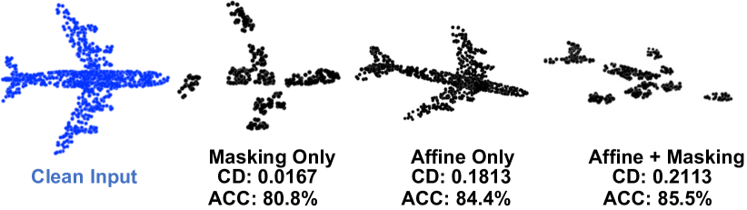
Figure 1: Visualizations of masking (e.g., Drop-Local) and affine transformation (e.g., Affine) corruptions and the corresponding Chamfer Distance (CD) to the clean input, where the reported CD values are averaged over the ShapeNet training set. The ACC reports the classification accuracy on downstream ScanObjectNN dataset, as detailed in Tab. I.

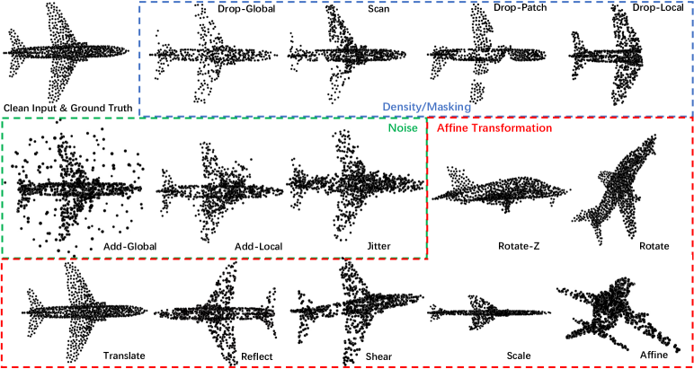
Figure 2: Illustration of the $14$ corruptions studied in this work, which can be classified into three corruption families, i.e., density/masking, noise, and affine transformation. Please refer to the supplementary material for more detailed implementation of these corruptions.

By analyzing these pretext tasks, we identify another effective corruption family, i.e., affine transformation, in addition to the popular masking strategy. With affine transformation, we disturb all points with a specific transformation matrix globally. Such a global transformation introduces considerable shape deformation, as revealed by the enlarged CD in Fig. 1. Considering that the masking corruption drops partial points of local regions while the affine transformation introduced global distortion, better results are expected by combining these two complementary corruption types, as justified in Tab. I.

While it is direct to apply the affine transformation to the traditional non-Transformer backbones, introducing it to the Transformer backbones is non-trivial. Specifically, existing Transformer-based methods [7, 8] typically adopt unordered point patches as input and reconstruct the local point patches guided by their global position, e.g., the patch centers via positional embedding. Such leakage of global position impedes the perception of global shape during pre-training. This is even more serious with the affine transformation corruption, where the deformed global shape is directly indicated by the leaked global position, diluting the influence of affine transformation. To tackle this problem, we propose a simple approach to decompose the reconstruction of the complete point cloud into the reconstructions of detailed local patches and rough global shape. By modeling the global shape explicitly, the effectiveness of global affine transformation is fully utilized and improved model representation can be achieved, as presented in Tab. X.

We carefully analyze the proposed components and validate the effectiveness of our Point-DAE on a wide range of downstream tasks. Specifically, we testify the complementarity between corruptions of masking and affine transformation on both Transformer and non-Transformer encoders. With frozen encoders, Point-DAE achieves 87.9% and 84.6% classification accuracy on ScanObjectNN dataset with DGCNN and Transformer encoders, outperforming the second-best methods [15, 8] by 6.2% and 5.9%, respectively. When fine-tuning on downstream tasks, Point-DAE achieves 92.1% (+8.2%) accuracy on ScanObjectNN for shape classification, 86.0% (+0.5%) instance mIoU on ShapeNetPart for part segmentation, 93.0% (+9.4%) few-shot classification accuracy on 10-way 10-shot on ModelNet40, and 0.835 mCE (-0.165 mCE) on ModelNet-C for robustness testing with the DGCNN encoder. Similar improvements are achieved with the Transformer backbone, validating the generality of our method. We summarize our contributions as follows:

• We investigate a general denoising autoencoder framework for self-supervised point cloud learning (Point-DAE) by exploring three corruption families (e.g., density/masking, noise, and affine transformation) and a total of fourteen corruption types. By analyzing these variants, we identify another effective corruption family, i.e., affine transformation, which is complementary to the popular masking strategy.

• We validate the effectiveness of the revealed affine transformation corruption on various backbone encoders, including the non-Transformer and Transformer ones. For the Transformer-based Point-DAE, we propose a reconstruction decomposition strategy to tackle the position leakage problem occurred in the reconstruction.

• We carefully ablate the proposed components and validate the pre-trained models with extensive downstream tasks, including object classification, few-shot learning, robustness testing, part segmentation, and 3D object detection. We also present intuitive reconstruction visualization and some interesting observations, such as the influence of object poses in the pre-training dataset.

II Related Work

Pre-training by Reconstruction. Feature learning via sample reconstruction has a long research history [16, 14]. Recently, masked modeling has gained increasing attention in multiple data modalities, where we mask some parts of the data signals as input and learn an encoder-decoder model to reconstruct the masked data. The pioneering masked language modeling has achieved a significant performance boost on downstream tasks [17, 18]. Inspired by this, masked image modeling [19, 6] and masked video modeling [9, 20] are actively investigated and present considerable successes. Recently, masked modeling is also explored in the point cloud domain with irregular data input. An initial attempt masks points via view occlusion [10], and recent works mask point patches with the Transformer backbone [21]. Given discrete tokens from point patches via dVAE [22], Point-BERT [7] reconstructs masked tokens with a contrastive objective. Without dVAE mapping, Point-MAE [8] and Point-M2AE [11] reconstruct the masked point patches directly with a pure masked autoencoding framework. Besides explicit points, the target of implicit 3D representations, such as occupancy value and signed distance function, is also studied given masked point cloud [12, 23]. Unlike these masked modeling methods that only corrupt points by masking local regions, we investigate a more general denoising autoencoder by conducting sample corruption in a broader space. With such a comprehensive study, we recommend to use another global affine transformation corruption to complement the local masking strategy, leading to more effective and robust feature representation for point clouds.

Self-supervised Point Cloud Learning. The performance of point cloud learning has been boosted with carefully designed model architectures and optimization strategies under the supervised learning context [24, 25, 26, 27, 28, 29, 30, 31, 32, 33, 34, 35]. In this work, we explore an orthogonal SSL direction to learn effective feature representations from unlabeled point cloud data. Pretext tasks such as Jigsaw [2] and orientation estimation [36] are explored in pioneering attempts. One mainstream pipeline is contrastive learning, which minimizes the distance between different ‘views’ of the same sample and maximizes the distance across different samples. The required sample view can be introduced via different modalities [15], data augmentation [5, 37], view occlusion [38], and local structure [39]. Some recent methods [40, 41] require additional knowledge from pretrained models of other modalities, resulting in unfair advantages. Reconstruction is another popular SSL framework, which reconstructs the clean point cloud from its corrupted version. The corrupted point cloud can be generated by part disorganization [42], contour perturbation [43], and masking [10, 7, 8, 11]. Most of these corruptions only corrupt partial points of the input, while other points remain unchanged. In contrast, we promote using affine transformation to corrupt all input points globally. We validate the complementary between the popular masking and the studied affine transformation on various encoders and achieve state-of-the-art performance on wide downstream tasks.

Sample corruptions. Sample corruptions have been widely investigated in different research areas. Data augmentation via sample corruptions has demonstrated its effectiveness in settings of both independent and identical distribution [44, 45] and our-of-distribution (OOD) [46]. The dataset for testing OOD generalization performance is typically generated by applying corruptions to clean samples [47, 48]. Sample corruptions also play important roles in semi-supervised learning [49] and contrastive learning [3]. In low-level vision tasks (e.g., image super-resolution [50] and point cloud upsampling [51]), training pairs are typically constructed by applying corruptions to high-quality samples. However, the objective in low-level vision tasks is mainly to reconstruct high-quality samples, while the main objective of SSL is to learn effective feature representations without manual annotations.

III Our Approach

We first present an overview of the proposed Point-DAE method. Then we present how to implement it with non-Transformer and Transformer encoders, respectively.

III-A Overview of Point-DAE

The Point-DAE method can be summarized as follows:

$$\min_{\mathrm{E},\mathrm{D}}\mathbb{E}_{\mathbf{X}\in\mathbb{X}}\mathcal{L}\left(\mathrm{D}(\mathrm{E}(\mathrm{Corruption}(\mathbf{X}))),\mathbf{X}\right),$$ (1)

where $\mathbf{X}\in\mathbb{R}^{w\times 3}$ is a point cloud in the dataset $\mathbb{X}$. $\mathrm{E}(\cdot)$ and $\mathrm{D}(\cdot)$ represent the encoder and decoder models, respectively. $\mathrm{Corruption}(\cdot)$ indicates the applied corruption (e.g., masking and affine transformation). $\mathcal{L}(\cdot,\cdot)$ is the loss function measuring the reconstruction quality, which is set as the popular CD loss [52] by default:

$$\mathcal{L}_{cd}(\widehat{\mathbf{X}},\mathbf{X})=\frac{1}{w}\sum_{\mathbf{x}\in\mathbf{X}}\min_{\widehat{\mathbf{x}}\in\widehat{\mathbf{X}}}\|\mathbf{x}-\widehat{\mathbf{x}}\|_{2}^{2}+\frac{1}{\widehat{w}}\sum_{\widehat{\mathbf{x}}\in\widehat{\mathbf{X}}}\min_{\mathbf{x}\in\mathbf{X}}\|\mathbf{x}-\widehat{\mathbf{x}}\|_{2}^{2},$$ (2)

where $\widehat{\mathbf{X}}\in\mathbb{R}^{\widehat{w}\times 3}$ is the reconstructed point cloud. $\mathbf{x}\in\mathbb{R}^{3}$ and $\widehat{\mathbf{x}}\in\mathbb{R}^{3}$ are points in $\mathbf{X}$ and $\widehat{\mathbf{X}}$, respectively. We explore Point-DAE on various encoder backbones, which can be roughly clustered into two clans, i.e., the non-Transformer clan that processes the global point cloud as a whole [53, 54, 55] and the Transformer clan that divides the whole point cloud into local patches as input [7, 8, 11]. The corresponding implementations are illustrated in Fig. 3 and detailed in the following sections.

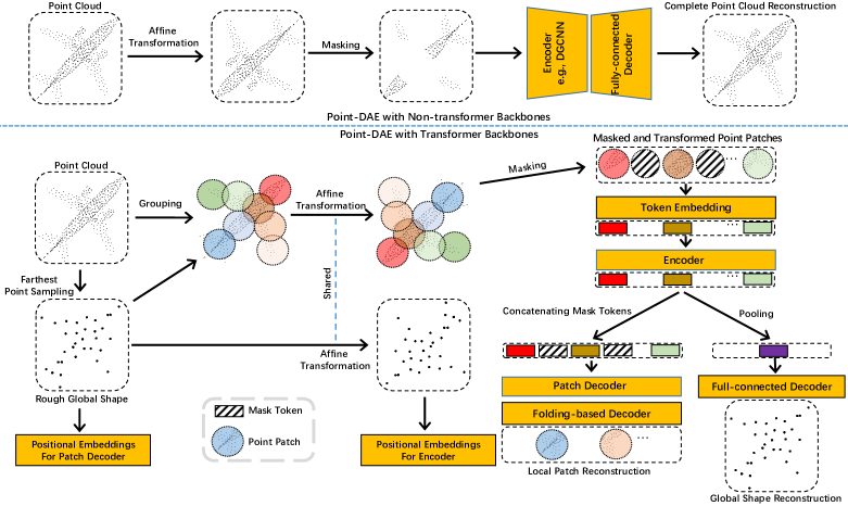
Figure 3: An overview of Point-DAE with non-Transformer backbones (upper part) and Transformer backbones (lower part), where we use a toy rotation operation to represent the affine transformation for visualization.

The corruption $\mathrm{Corruption}(\cdot)$ is our focus in this work, given that each type of corruption instantiates a unique pretext task. Inspired by the practice of [56, 48], we systemically investigate three corruption families (i.e., density/masking, noise, and affine transformation) and a total of $14$ corruption types. Generally speaking, we randomly change the point density either uniformly or nonuniformly to implement the density/masking corruptions, and add random noises to the point cloud either locally or globally to implement the noise corruptions. The affine transformation corruptions are implemented by multiplying the augmented input with a random affine transformation matrix as follows:

$$\left[\begin{array}[]{c}x^{\prime}\\ y^{\prime}\\ z^{\prime}\\ 1\\ \end{array}\right]=\left[\begin{array}[]{cccc}a_{11}&a_{12}&a_{13}&a_{14}\\ a_{21}&a_{22}&a_{23}&a_{24}\\ a_{31}&a_{32}&a_{33}&a_{34}\\ 0&0&0&1\\ \end{array}\right]\left[\begin{array}[]{c}x\\ y\\ z\\ 1\\ \end{array}\right],$$ (3)

where $[x,y,z]$ and $[x^{\prime},y^{\prime},z^{\prime}]$ are the input and transformed points, respectively. The affine transformation matrix is defined by the $12$ parameters, i.e., $a_{ij}$, covering the Rotate, Translate, Reflect, Shear, and Scale sub-transformations with various magnitudes, as analyzed in the supplementary material.

The representative corruptions are visualized in Fig. 2. One can see that we implement four corruptions for density/masking family, three corruptions for noise family, and seven corruptions for affine transformation family, resulting in 14 types of corruptions in total. Although we practically investigate all the 14 corruption types in Sec. IV, we only introduce the detailed implementation of the most effective variant, i.e., Point-DAE with affine transformation and masking corruptions, on different encoder backbones in the following sections.

III-B Point-DAE with Non-Transformer Encoders

Training Data Preparation. Given a point cloud $\mathbf{X}\in\mathbb{R}^{w\times 3}$, we first generate its affine transformed counterpart $\mathbf{X}^{\prime}\in\mathbb{R}^{w\times 3}$ by applying the random affine transformation matrix of Eq. (3) to $\mathbf{X}$ in a point-wise manner.

Then, we mask some points from $\mathbf{X}^{\prime}$. Existing approaches typically mask points occluded in a camera view [10] or drop fixed-sized KNN clusters [8]. Unlike these methods, we promote a more effective strategy, i.e., Drop-Local, by masking several random-sized KNN clusters. Specifically, we first randomly set the number of dropped clusters $\kappa\in\mathbb{Z}^{+}$ and the total number of dropped points $\eta=\lfloor\alpha w\rfloor$, where $\alpha\in(0,1)$ is the masking ratio. Then, for the $i$-th cluster, we randomly select a point in $\mathbf{X}^{\prime}$ as the cluster center and drop its nearest $\eta_{i}$ points, where $\sum_{i=1}^{\kappa}\eta_{i}=\eta$ and $\eta_{i}>0$. Finally, we get the masked and affine transformed $\mathbf{X}^{\prime}_{mask}$.

Encoder. The encoder takes the $\mathbf{X}^{\prime}_{mask}$ as input and outputs a global feature $\mathbf{F}^{\prime}_{e}\in\mathbb{R}^{d}$:

$$\mathbf{F}^{\prime}_{e}=\mathrm{E}(\mathbf{X}^{\prime}_{mask}).$$ (4)

The encoder $\mathrm{E}(\cdot)$ can be instantiated as any point cloud encoders [53, 54, 55], including the recent Transformer-based ones [7, 11, 28]. However, we promote a more effective implementation of Point-DAE for the Transformer backbones, as detailed in Sec. III-C.

Decoder. Given the encoded feature $\mathbf{F}^{\prime}_{e}$, an decoder is learned to reconstruct the original point cloud $\mathbf{X}$. Inspired by the practice of point cloud reconstruction, we investigate two types of decoders, i.e., the fully-connected decoder $\mathrm{D}_{fc}$ [57, 58] and the folding-based decoder $\mathrm{D}_{fold}$ [59]. Specifically, the $\mathrm{D}_{fc}$ transforms $\mathbf{F}^{\prime}_{e}$ into a vector of $3w$ elements with fully connected (FC) layers and reshapes it to reconstruct the point cloud $\widehat{\mathbf{X}}\in\mathbb{R}^{w\times 3}$:

$$\widehat{\mathbf{X}}=\mathrm{D}_{fc}(\mathbf{F}^{\prime}_{e})=\mathrm{Reshape}\left(FC(\mathbf{F}^{\prime}_{e})\right).$$ (5)

The folding-based decoder $\mathrm{D}_{fold}$ [59] generates the point cloud by deforming a canonical 2D grid $\mathbf{G}\in\mathbb{R}^{w\times 2}$ conditioned on the global feature $\mathbf{F}^{\prime}_{e}$:

$$\widehat{\mathbf{X}}=\mathrm{D}_{fold}(\mathbf{F}^{\prime}_{e})=\mathrm{MLP}(\mathrm{Concat}[\mathbf{G},\mathbf{F}^{\prime}_{e}]),$$ (6)

where $\mathrm{Concat}[\mathbf{G},\mathbf{F}^{\prime}_{e}]\in\mathbb{R}^{w\times(d+2)}$ concatenates the 2D grid $\mathbf{G}$ and the replicated global feature $\mathbf{F}^{\prime}_{e}$, and $\mathrm{MLP}(\cdot):\mathbb{R}^{w\times(d+2)}\to\mathbb{R}^{w\times 3}$ constructs the point cloud with multi-layer perceptrons (MLP).

The decoder architecture also plays an important role in SSL, which is less studied. We find that the fully-connected decoder $\mathrm{D}_{fc}$ performs better in complete/global shape reconstruction, while the folding-based decoder $\mathrm{D}_{fold}$ shows advantages on modeling smooth local patches (please refer to Sec. III-C and Sec. IV for more details).

Final Loss. We adopt the CD loss in Eq. (2) to measure the reconstruction divergence between $\mathbf{X}$ and $\widehat{\mathbf{X}}$, resulting in the following loss function:

$$\mathcal{L}_{all}=\mathcal{L}_{cd}(\widehat{\mathbf{X}},\mathbf{X}).$$ (7)

III-C Point-DAE with Transformer Encoders

Instead of reconstructing the complete point cloud directly as in Sec. III-B, we decompose the overall reconstruction task into the reconstructions of detailed local patches and rough global shape for Transformer backbones, which is detailed in the following content.

Training Data Preparation. Given a point cloud $\mathbf{X}\in\mathbb{R}^{w\times 3}$, we first sample $n$ points as patch centers $\mathbf{C}\in\mathbb{R}^{n\times 3}$ via the Farthest Point Sampling method [54]. Then the point patches $\mathbf{P}\in\mathbb{R}^{n\times k\times 3}$ are formed by searching the $K$ nearest points around each patch center using the KNN method. Then, we apply the masking and affine transformation corruptions to the point patches $\mathbf{P}$ in a patch-wise manner. Specifically, we first generate the affine transformed patches $\mathbf{P}^{\prime}\in\mathbb{R}^{n\times k\times 3}$ and patch centers $\mathbf{C}^{\prime}\in\mathbb{R}^{n\times 3}$ by applying certain affine transformation matrix (cf. Eq. (3)) to $\mathbf{P}$ and $\mathbf{C}$ in a point-wise manner. Then, we normalize each point patch in $\mathbf{P}^{\prime}$ and $\mathbf{P}$ by subtracting its patch center from the point coordinates.

Given the point patches $\mathbf{P}^{\prime}$, we randomly mask a large portion of them to conduct the masking corruption. Specifically, we mask out $m=\lfloor\alpha n\rfloor$ patches to obtain the masked patches $\mathbf{P}^{\prime}_{mask}\in\mathbb{R}^{m\times k\times 3}$ and unmasked patches $\mathbf{P}^{\prime}_{vis}\in\mathbb{R}^{(n-m)\times k\times 3}$, where $\alpha\in(0,1)$ is the masking ratio. The corresponding masked patch centers $\mathbf{C}^{\prime}_{mask}\in\mathbb{R}^{m\times 3}$ and unmasked patch centers $\mathbf{C}^{\prime}_{vis}\in\mathbb{R}^{(n-m)\times 3}$ are similarly obtained for the usage of positional embedding (PE). With the same masking strategy, the corresponding masked patches $\mathbf{P}_{mask}\in\mathbb{R}^{m\times k\times 3}$, unmasked patches $\mathbf{P}_{vis}\in\mathbb{R}^{(n-m)\times k\times 3}$, masked patch centers $\mathbf{C}_{mask}\in\mathbb{R}^{m\times 3}$, and unmasked patch centers $\mathbf{C}_{vis}\in\mathbb{R}^{(n-m)\times 3}$ from $\mathbf{P}$ and $\mathbf{C}$ are also generated.

The transformed and unmasked patches $\mathbf{P}^{\prime}_{vis}$ and their centers $\mathbf{C}^{\prime}_{vis}$ are used as the input to the Transformer-based encoder. The vanilla patch centers $\mathbf{C}$ are adopted as the supervision of global shape reconstruction and the PE for the Transformer-based patch decoder. The vanilla masked patches $\mathbf{P}_{mask}$ are adopted as the supervision signal for local patches reconstruction. The details are presented in the following subsections.

Token Embedding. Before feeding the unmasked point patches into the Transformer-based encoder, we transform them into tokens via a simple PointNet, which consists of an MLP and a max pooling layer. Specifically, we introduce the embedded visible tokens $\mathbf{T}^{\prime}_{vis}\in\mathbb{R}^{(n-m)\times d}$ as:

$$\mathbf{T}^{\prime}_{vis}=\mathrm{MaxPooling}(\mathrm{MLP}(\mathbf{P}^{\prime}_{vis})),$$ (8)

where the MLP is applied to the feature dimension while the max pooling is conducted across the $k$ neighboring points.

Encoder. The encoder is built with the standard Transformer blocks [21]. Following the common practice, we only feed the visible tokens into the encoder to reduce the computational complexity [8]. We add the input tokens with the token-wise PE in each Transformer block because the coordinates in point patches are normalized. Finally, the encoded tokens $\mathbf{T}^{\prime}_{e}\in\mathbb{R}^{(n-m)\times d}$ are introduced as:

$$\mathbf{T}^{\prime}_{e}=\mathrm{E}(\mathbf{T}^{\prime}_{vis},\mathbf{T}_{pe}^{e}(\mathbf{C}^{\prime}_{vis})),$$ (9)

where $\mathbf{T}_{pe}^{e}:\mathbb{R}^{(n-m)\times 3}\to\mathbb{R}^{(n-m)\times d}$ is constructed with a learnable MLP and it maps coordinates of patch centers to the feature dimension $d$.

Decoder. Motivated by the methods that reconstruct the complete point cloud in a patch-wise manner [7, 8], we promote to decompose the reconstruction of the whole point cloud $\mathbf{X}$ into the reconstructions of detailed local patches and rough global shape. Given the encoded visible tokens $\mathbf{T}^{\prime}_{e}$ and the learnable mask tokens $\mathbf{T}_{m}\in\mathbb{R}^{m\times d}$, the patch decoder $\mathrm{D}_{patch}$ predicts the decoded mask tokens $\mathbf{T}_{d}\in\mathbb{R}^{m\times d}$ as:

$$\mathbf{T}_{d}=\mathrm{D}_{patch}(\mathbf{T}^{\prime}_{e},\mathbf{T}_{m},\mathbf{T}_{pe}^{d}(\mathbf{C})),$$ (10)

where we duplicate the $d$-dimensional learnable mask token to construct $\mathbf{T}_{m}$ and the decoder PE, i.e., $\mathbf{T}_{pe}^{d}:\mathbb{R}^{n\times 3}\to\mathbb{R}^{n\times d}$ share the same structure as the encoder PE of $\mathbf{T}_{pe}^{e}$. We adopt two separate PEs for encoder and patch decoder since they respectively receive transformed patch centers $\mathbf{C}^{\prime}_{vis}$ and vanilla patch centers $\mathbf{C}$. The patch decoder $\mathrm{D}_{patch}(\cdot)$ is also constructed with the standard Transformer [21] but with fewer blocks compared to the encoder. Note that $\mathbf{T}^{\prime}_{e}$ is the encoded tokens of corrupted point cloud patches, while $\mathbf{T}_{pe}^{d}(\mathbf{C})$ and $\mathbf{T}_{d}$ are the PEs and decoded tokens for the uncorrupted patches, respectively. In other words, we reconstruct the uncorrupted tokens from their corrupted counterparts guided by the uncorrupted patch centers $\mathbf{C}$.

Given the decoded mask tokens $\mathbf{T}_{d}$, we predict their corresponding point cloud patches via the folding-based decoder head in Eq. (6):

$$\widehat{\mathbf{P}}_{mask}=\mathrm{D}_{fold}(\mathbf{T}_{d}),$$ (11)

where $\mathrm{D}_{fold}(\cdot):\mathbb{R}^{m\times d}\to\mathbb{R}^{m\times k\times 3}$ decodes each patch feature in $\mathbf{T}_{d}$ as a point cloud patch. For paired point cloud patches in the reconstructed $\widehat{\mathbf{P}}_{mask}$ and the ground truth $\mathbf{P}_{mask}$, we measure the reconstruction quality via the CD loss in Eq. (2). The reconstruction loss of local patches are averaged over the $m$ masked patches:

$$\mathcal{L}_{local}=\frac{1}{m}\sum_{i=1}^{m}\mathcal{L}_{cd}(\mathbf{P}_{mask}^{i},\widehat{\mathbf{P}}_{mask}^{i}),$$ (12)

where $\mathbf{P}_{mask}^{i}\in\mathbb{R}^{k\times 3}$ and $\widehat{\mathbf{P}}_{mask}^{i}\in\mathbb{R}^{k\times 3}$ are the $i$-th point patch in $\mathbf{P}_{mask}$ and $\widehat{\mathbf{P}}_{mask}$, respectively.

It should be noted that the objective $\mathcal{L}_{local}$ in Eq. (12) only measures the reconstruction performance of normalized local patches, given that the rough global shape is fed into the patch decoder via PE, e.g., $\mathbf{C}$. In other words, the PE leaks the positions of the global shape. While this is a common practice in existing methods [7, 8], we argue that the reconstruction of global shape is also important for the reconstruction of a complete point cloud, especially when its global information is corrupted by the affine transformation. Therefore, we introduce the following global shape reconstruction loss $\mathcal{L}_{global}$ to complement the local patch reconstruction:

$$\mathcal{L}_{global}=\mathcal{L}_{cd}(\widehat{\mathbf{C}},\mathbf{C}),$$ (13)

where $\widehat{\mathbf{C}}\in\mathbb{R}^{n\times 3}$ contains the predicted patch centers (e.g., rough global shape) from encoded tokens $\mathbf{T}^{\prime}_{e}$ in Eq. (9):

$$\widehat{\mathbf{C}}=\mathrm{D}_{fc}(\mathrm{Pooling}(\mathbf{T}^{\prime}_{e})),$$ (14)

where $\mathrm{Pooling}(\cdot):\mathbb{R}^{(n-m)\times d}\to\mathbb{R}^{d}$ merges patch features into a global feature and $\mathrm{D}_{fc}(\cdot):\mathbb{R}^{d}\to\mathbb{R}^{n\times 3}$ is the fully-connected decoder detailed in Eq. (5).

Final Loss. By decomposing the reconstruction of whole point cloud into the reconstructions of local patches in Eq. (12) and global shape in Eq. (13), we have the following final loss function:

$$\mathcal{L}_{all}=\mathcal{L}_{local}+\lambda\mathcal{L}_{global},$$ (15)

where $\lambda$ is a hyper-parameter balancing the two loss terms.

IV Experiments

We perform extensive experiments on downstream tasks of point cloud learning with various encoder backbones. The Point-DAE variants with different types of corruptions are first investigated and then we compare our method against current state of the arts on extensive downstream tasks.

IV-A Self-supervised Pre-training

For most downstream tasks except for the 3D object detection, we conduct self-supervised pre-training on the ShapeNet dataset [60], which contains about $51$K samples shared by $55$ categories, following [10, 7, 8]. For the 3D object detection, we follow [12] to pre-train our model with the ScanNetv2 dataset [61], which includes $1,201$, $312$, and $100$ scenes for training, validation, and test, respectively. We validate our Point-DAE with point cloud encoders of PointNet [53], PointNet++ [54], DGCNN [55], standard Transformer [7, 8], and the hierarchical Transformer [11]. Especially, for standard Transformer, we construct the encoder and decoder with $12$ and $4$ Transformer blocks, respectively. Each Transformer block contains $384$ dimension and $6$ heads. For the hierarchical Transformer encoder, we follow [11] to adopt multi-scale masking and a hierarchical patch decoder. The AdamW optimizer [62] and the cosine learning rate schedule [63] are used to train the network. The total training epochs, initial learning rate, and number of points are respectively set as $300$, $0.001$, and $1024$ unless otherwise specified.

TABLE I: Results of different variants of Point-DAE on the ScanObjectNN dataset with the ObjBG setting. The linear probing protocol is used.

	Corruptions	PointNet	PointNet++	DGCNN
	$\blacktriangledown$ No-Corruption	75.7$\pm$0.9	76.2$\pm$0.9	77.1$\pm$0.3
	$\clubsuit$ Drop-Global	74.4$\pm$0.2	77.3$\pm$0.5	76.4$\pm$0.2
	$\clubsuit$ Scan	77.0$\pm$0.1	78.1$\pm$1.2	78.9$\pm$0.3
	$\clubsuit$ Drop-Patch	72.7$\pm$0.4	80.6$\pm$1.1	77.4$\pm$1.0
Masking	$\clubsuit$ Drop-Local	73.6$\pm$0.4	78.5$\pm$0.7	80.8$\pm$0.8
	$\blacklozenge$ Add-Global	73.6$\pm$0.3	77.5$\pm$0.6	77.3$\pm$0.9
	$\blacklozenge$ Add-Local	74.9$\pm$0.7	76.5$\pm$0.5	77.2$\pm$0.3
Noise	$\blacklozenge$ Jitter	76.0$\pm$0.8	76.1$\pm$0.3	78.0$\pm$1.4
	$\spadesuit$ Shear	75.6$\pm$0.1	77.7$\pm$0.1	79.4$\pm$0.6
	$\spadesuit$ Rotate-Z	73.9$\pm$0.4	77.9$\pm$0.3	79.2$\pm$0.9
	$\spadesuit$ Translate	75.1$\pm$0.4	78.6$\pm$0.1	81.2$\pm$0.7
	$\spadesuit$ Scale	77.2$\pm$0.9	79.9$\pm$0.5	80.4$\pm$0.5
	$\spadesuit$ Reflect	78.3$\pm$0.7	81.8$\pm$0.3	82.8$\pm$0.3
	$\spadesuit$ Rotate	76.2$\pm$0.1	80.6$\pm$0.8	82.8$\pm$0.5
Affine Trans.	$\spadesuit$ Affine	77.4$\pm$0.7	84.9$\pm$1.0	84.4$\pm$0.3
	Affine
	$\bigstar$ + Drop-Patch	74.8$\pm$0.1	86.0$\pm$0.6	84.8$\pm$0.1
Comb.	$\bigstar$ + Drop-Local	75.6$\pm$0.5	87.0$\pm$0.7	85.5$\pm$0.7
	$\blacksquare$ Supervised	78.3$\pm$0.2	87.0$\pm$0.1	86.8$\pm$0.2

TABLE II: Results of Point-DAE on the ScanObjectNN dataset with the ObjBG setting under the linear probing protocol, where the Transformer encoder is used.

Corruptions	Accuracy (%)
$\blacktriangledown$ No-Corruption	76.9$\pm$0.5
$\clubsuit$ Drop-Patch	82.7$\pm$0.7
$\spadesuit$ Affine	79.8$\pm$0.5
$\bigstar$ Affine + Drop-Patch	84.6$\pm$0.6

IV-B Point-DAE Variants with Different Corruptions

We first study the Point-DAE variants with seminal non-Transformer encoders, e.g., PointNet [53], PointNet++ [54], and DGCNN [55], and then verify the findings with Transformer encoders. Specifically, we adopt a light-weighted PointNet architecture by removing the transformation modules since the transformation modules (i.e., T-Net) in PointNet are incompatible with the affine transformation corruption (refer to Sec. IV-D for more details). Besides the Point-DAE variants induced by the $14$ analyzed corruptions, we introduce the vanilla autoencoder (i.e., Point-DAE with ‘No-Corruption’ input) as the baseline, and explore the Point-DAE variants with combined corruptions. To compare Point-DAE with supervised pre-training, we introduce the ‘Supervised’ setting by learning the encoder with manual category labels. We run each variant with three random seeds and report the mean and standard deviation of the results. We adopt the same experimental setting across different Point-DAE variants to ensure a fair comparison.

Results of Point-DAE variants with different corruption types are illustrated Tab. I. Firstly, different corruption types lead to different pretext tasks, resulting in a significant divergence on the downstream performance. For example, masking points nonuniformly (e.g., Drop-Local) typically leads to better performance over uniform point masking (e.g., Drop-Global). Adding noise is a less effective corruption operation, while the affine transformation corruption boosts the results significantly. Combining the revealed affine transformation corruption and the popular masking one leads to consistent improvement with the backbones of PointNet++ and DGCNN, validating their complementarity. Secondly, the same input corruption may lead to opposite effects for different model architectures. For instance, the popular local point masking strategy (e.g., Drop-Patch or Drop-Local) leads to different results with different model architectures. For PointNet++ and DGCNN, which are designed with local perception modules, randomly masking the local part of the input introduces explicit regularization, benefiting the extraction and aggregation of local features. Therefore, more effective feature representation can be learned with corruptions of local point masking. On the contrary, masking local points brings a significant negative impact on PointNet, where the global information is overly weighted than local knowledge. Interestingly, the affine transformation corruption brings consistent improvement, revealing that enhancing the global shape perception is important for all model architectures.

The general message in Tab. I is the effectiveness of the affine transformation corruption and its complementarity to the popular masking strategy. Then, we validate whether these conclusions also hold with the prevalent Transformer backbone, as presented in Tab. II. One may note that affine transformation presents advantages with the non-Transformer encoders while the masking corruption (e.g., Drop-Patch) performs better with the Transformer architecture. This could be attributed to the architecture character, where the patch-wise masking and reconstruction strategy fits the patch-wise processing of the Transformer. Nevertheless, the complementarity between the masking and affine transformation holds with both Transformer and non-Transformer encoders.

TABLE III: Linear probing results on ModelNet40 dataset. The ‘S’ and ‘H’ in column ‘Encoder’ indicate the standard Transformer without any special design and the Transformer with hierarchical structure, respectively.

Methods	#Points	PointNet	DGCNN
Self-Contrast [64]	1K	–	89.6
OcCo [10]	1K	88.7	89.2
Jigsaw [2]	–	87.3	90.6
Poursaeed et al. [36]	1K	88.6	90.8
STRL [65]	2K	88.3	90.9
CrossPoint [15]	1K	89.1	91.2
Point-DAE (Ours)	1K	89.4	92.1

(a) Non-Transformer backbones.

Methods	#Points	Encoder	Accuracy (%)
Point-MAE [8]	1K	S	90.6
Point-DAE (Ours)	1K	S	92.2
Point-M2AE [11]	1K	H	92.9
Point-DAE (Ours)	1K	H	93.1

(b) Transformer backbones.

TABLE IV: Classification results on ScanObjectNN dataset.

Supervised References	OBJ-BG Results
PointNet++ [54]	82.3
PointCNN [24]	86.1
SSL Methods	PointNet	DGCNN
Fine-tuning Protocol
From Scratch	73.3	82.4
+ Jigsaw [2]	76.5	82.7
+ OcCo [10]	80.0	83.9
+ PointVST [66]	–	89.3
+ IAE [23]	–	90.2
+ Point-DAE (Ours)	80.2	92.1
Linear Probing Protocol
Jigsaw [2]	55.2	59.5
OcCo [10]	69.5	78.3
CrossPoint [15]	75.6	81.7
Point-DAE (Ours)	78.1	87.9

(a) Non-Transformer backbones

Methods	OBJ-BG	OBJ-ONLY	PB-T50-RS
Fine-tuning Protocol
Standard Transformer [7]	79.86	80.55	77.24
+ OcCo [10, 7]	84.85	85.54	78.79
+ Point-BERT [7]	87.43	88.12	83.07
+ Point-GAME [67]	88.99	87.95	83.79
+ MaskPoint [12]	89.3	89.7	84.6
+ Point-MAE [8]	90.02	88.29	85.18
+ Point-CAM [68]	90.36	88.35	84.49
+ TAP [69]	90.36	89.50	85.67
+ Joint-MAE [70]	90.94	88.86	86.07
+ MAE3D [71]	–	–	86.20
+ Point2vec [72]	91.2	90.4	87.5
+ ACT [73]	93.29	91.91	88.21
+ Point-DAE (Ours)	93.63	92.77	88.69
Hierarchical Transformer [11]	82.31	81.57	79.35
+ Point-M2AE [11]	91.22	88.81	86.43
+ IAE [23]	92.5	91.6	88.2
+ Point-DAE (Ours)	93.86	93.07	89.31
Linear Probing Protocol
Point-MAE [8]	80.13	80.62	70.41
Point-DAE (Ours)	84.62	84.73	74.62

(b) Transformer backbones

IV-C Results on Downstream Tasks

We adopt the following two protocols to validate the pre-trained encoder on downstream tasks:

• Fine-tuning protocol, where we fine-tune both the pre-trained encoder and the randomly initialized classification head on downstream tasks.

• Linear probing protocol, where we freeze the pre-trained encoder and learn a linear support vector machine (SVM) classifier on the extracted features.

In the following studies, results of competitors are either copied from the original papers or quoted from [10, 15].

Object Classification. We validate our method on object classification datasets of ModelNet40 and ScanObjectNN. The widely-used ModelNet40 dataset [74] includes about $12K$ synthetic objects shared by $40$ categories, while the challenging ScanObjectNN dataset [75] consists of about $15K$ scanned point cloud instances shared by $15$ classes. As shown in Tab. III, Point-DAE consistently outperforms the competitors on the ModelNet40 dataset with various encoder backbones. On the challenging ScanObjectNN dataset, our Point-DAE shows more considerable advantages, as illustrated in Tab. IV.

Our method also achieves better performance with more powerful backbones, as shown by the comparison between PointNet and DGCNN, and standard and hierarchical Transformers. The advantages with different backbones, on different datasets, and under different evaluation protocols fully justify the effectiveness and generality of our method. We provide the ModelNet40 results [74] under the fine-tuning protocol in the Supplementary Material since performance on this simple task is already saturated (i.e., around 94% accuracy).

TABLE V: Robustness to common corruptions on the ModelNet-C test dataset.

Methods	OA $\uparrow$	mCE $\downarrow$	Scale	Jitter	Drop-G	Drop-L	Add-G	Add-L	Rotate
DGCNN (From Scratch)	0.926	1.000	1.000	1.000	1.000	1.000	1.000	1.000	1.000
+ OcCo [10]	0.922	1.047	1.606	0.652	0.903	1.039	1.444	0.847	0.837
+ Point-DAE (Ours)	0.933	0.835	0.957	0.883	0.944	0.841	0.668	0.815	0.736

Robustness Testing. We study the model robustness to sample corruptions on the ModelNet-C test set [76], which is constructed by applying seven atomic corruptions to the vanilla ModelNet40 test set. Among the seven studied corruptions, corruptions similar to Scale, Rotate, and Drop-L have been utilized in the pre-training stage of Point-DAE, while the other four corruptions of Jitter, Drop-G, Add-G, and Add-L have not been exposed. In the fine-tuning stage, we strictly follow the evaluation protocol of [76] and only use conventional augmentations of scaling and translation. Besides the overall accuracy (OA) on the clean test set, we report the mean Corruption Error (mCE) for the robustness evaluation. As illustrated in Tab. V, Point-DAE outperforms the vanilla DGCNN on the clean test set and achieves improved robustness to all the seven investigated corruptions. Especially the results on Jitter, Drop-G, Add-G, and Add-L corruptions validate its improved generalization capability to unseen corruptions.

Robustness to SO(3) Rotation. Although the model robustness to rotations has been preliminarily investigated with the ModelNet-C test set, it is restricted to small angle ranges [76]. In this analysis, we investigate the Point-DAE in the more challenging setting of arbitrary SO(3) rotations [77, 78, 79]. Specifically, we adopt two experiment settings with the DGCNN backbone following the common practice [77, 78, 79]. We randomly rotate the training and test data around the $z$-axis in the ‘$z/z$’ setting. In the ‘SO(3)/SO(3)’ setting, training and test data are randomly rotated around the $xyz$-axes. As illustrated in Tab. VI, Point-DAE improves over the DGCNN baseline on both settings, validating the improved rotation robustness to arbitrary SO(3) rotations.

TABLE VI: Classification results with different rotation settings. All comparing methods adopt ‘xyz’ input only.

Methods	$z/z$	SO(3)/SO(3)
ModelNet40
Rotation-specific Methods
SPHNet [77]	87.7	87.2
SFCNN [78]	91.4	90.1
RI-GCN [79]	89.5	89.5
DGCNN (From Scratch)	90.1	88.3
+ Point-DAE (Ours)	91.6	89.3
ObjBG setting of ScanObjectNN
DGCNN (From Scratch)	79.9	79.4
+ Point-DAE (Ours)	88.3	85.6

Part Segmentation We also validate Point-DAE on the part segmentation task with the ShapeNetPart dataset, which includes $16,881$ samples shared by $16$ classes. As illustrated in Tab. VII, our method outperforms previous methods by $+0.7\%$, $+0.5\%$, $+0.3\%$ with backbones of PointNet, DGCNN, and standard Transformer, respectively.

TABLE VII: Part segmentation results (mean IoU) on the ShapeNetPart dataset.

Methods	PointNet	DGCNN	Transformer
From Scratch	82.2	85.2	85.1
+ OcCo [10]	83.4	85.0	85.1
+ Jigsaw [2]	–	85.1	–
+ PointContrast [38]	–	85.3	–
+ CrossPoint [15]	–	85.5	–
+ Chen et al. [42]	84.1	–	–
+ Point-BERT [7]	–	–	85.6
+ MaskPoint [12]	–	–	86.0
+ Point-MAE [8]	–	–	86.1
+ Point-DAE (Ours)	84.8	86.0	86.4

3D Object Detection We also validate Point-DAE on the 3D objection detection task with the ScanNetv2 dataset [61], which includes $1,201$, $312$, and $100$ scenes for training, validation, and test, respectively. We closely follow [12] to conduct experiments for 3D object detection. Specifically, we pre-train our model on the ScanNet dataset, which includes about 2.5 million RGBD scans. Only the geometry information is utilized, while the RGB knowledge is discarded. We adopt the ‘ScanNet-Medium’ dataset, which is generated by sampling every $100$ frame from ScanNet and contains around $25$K samples. For each instance, we sample $20$K points and cluster them into $2,048$ groups, each containing $64$ points. We randomly mask $75\%$ of the groups as input to the Transformer encoder. The 3DETR model is adopted for the 3D objection detection task, where the encoder includes 3-layer self-attention blocks, and the decoder is composed of 8-layer cross-attention blocks. When fine-tuning, we strictly follow the 3DETR strategy, except that we initialize the encoder with the pre-trained weights. As illustrated in Tab. VIII, our method significantly improves over the 3DETR baseline (+2.0AP₂₅ and +4.9AP₅₀) and outperforms its closest competitor, Point-MAE, validating the effectiveness of Point-DAE on scene understanding.

TABLE VIII: 3D objection results on ScanNet validation set.

Methods	AP25	AP50
VoteNet [80]	58.6	33.5
+ PointContrast [38]	59.2	38.0
+ DepthContrast [37]	61.3	–
3DETR [81]	62.1	37.9
+ MaskPoint [12]	63.4	40.6
+ Point-MAE [8]	63.3	40.4
+ Point-DAE (Ours)	64.1	42.8

TABLE IX: Few-shot classification results with $1$K input points.

	5-way		10-way
	10-shot	20-shot	10-shot	20-shot
PointNet [53]	52.0$\pm$3.8	57.8$\pm$4.9	46.6$\pm$4.3	35.2$\pm$4.8
+ Jigsaw [2]	66.5$\pm$2.5	69.2$\pm$2.4	56.9$\pm$2.5	66.5$\pm$1.4
+ cTree [82]	63.2$\pm$3.4	68.9$\pm$3.0	49.2$\pm$1.9	50.1$\pm$1.6
+ OcCo [10]	89.7$\pm$1.9	92.4$\pm$1.6	83.9$\pm$1.8	89.7$\pm$1.5
+ CrossPoint [15]	90.9$\pm$4.8	93.5$\pm$4.4	84.6$\pm$4.7	90.2$\pm$2.2
+ Point-DAE (Ours)	93.0$\pm$3.7	94.9$\pm$3.3	86.7$\pm$5.8	92.1$\pm$4.6
DGCNN [55]	31.6$\pm$2.8	40.8$\pm$4.6	19.9$\pm$2.1	16.9$\pm$1.5
+ Jigsaw [2]	34.3$\pm$1.3	42.2$\pm$3.5	26.0$\pm$2.4	29.9$\pm$2.6
+ cTree [82]	60.0$\pm$2.8	65.7$\pm$2.6	48.5$\pm$1.8	53.0$\pm$1.3
+ OcCo [10]	90.6$\pm$2.8	92.5$\pm$1.9	82.9$\pm$1.3	86.5$\pm$2.2
+ CrossPoint [15]	92.5$\pm$3.0	94.9$\pm$2.1	83.6$\pm$5.3	87.9$\pm$4.2
+ Point-DAE (Ours)	96.7$\pm$2.5	97.7$\pm$1.6	93.0$\pm$4.8	95.6$\pm$2.6
Transformer [7]	87.8$\pm$5.2	93.3$\pm$4.3	84.6$\pm$5.5	89.4$\pm$6.3
+ OcCo [7]	94.0$\pm$3.6	95.9$\pm$2.3	89.4$\pm$5.1	92.4$\pm$4.6
+ Point-BERT [7]	94.6$\pm$3.1	96.3$\pm$2.7	91.0$\pm$5.4	92.7$\pm$5.1
+ MaskPoint [12]	95.0$\pm$3.7	97.2$\pm$1.7	91.4$\pm$4.0	93.4$\pm$3.5
+ Point-MAE [8]	96.3$\pm$2.5	97.8$\pm$1.8	92.6$\pm$4.1	95.0$\pm$3.0
+ Point-DAE (Ours)	96.8$\pm$2.4	98.3$\pm$1.5	93.2$\pm$4.6	95.6$\pm$3.2

(a) ModelNet40

	5-way		10-way
	10-shot	20-shot	10-shot	20-shot
PointNet [53]	57.6$\pm$2.5	61.4$\pm$2.4	41.3$\pm$1.3	43.8$\pm$1.9
+ Jigsaw [2]	58.6$\pm$1.9	67.6$\pm$2.1	53.6$\pm$1.7	48.1$\pm$1.9
+ cTree [82]	59.6$\pm$2.3	61.4$\pm$1.4	53.0$\pm$1.9	50.9$\pm$2.1
+ OcCo [10]	70.4$\pm$3.3	72.2$\pm$3.0	54.8$\pm$1.3	61.8$\pm$1.2
+ CrossPoint [15]	68.2$\pm$1.8	73.3$\pm$2.9	58.7$\pm$1.8	64.6$\pm$1.2
+ Point-DAE (Ours)	71.3$\pm$6.9	74.5$\pm$5.7	59.6$\pm$3.7	66.2$\pm$4.5
DGCNN [55]	62.0$\pm$5.6	67.8$\pm$5.1	37.8$\pm$4.3	41.8$\pm$2.4
+ Jigsaw [2]	65.2$\pm$3.8	72.2$\pm$2.7	45.6$\pm$3.1	48.2$\pm$2.8
+ cTree [82]	68.4$\pm$3.4	71.6$\pm$2.9	42.4$\pm$2.7	43.0$\pm$3.0
+ OcCo [10]	72.4$\pm$1.4	77.2$\pm$1.4	57.0$\pm$1.3	61.6$\pm$1.2
+ CrossPoint [15]	74.8$\pm$1.5	79.0$\pm$1.2	62.9$\pm$1.7	73.9$\pm$2.2
+ Point-DAE (Ours)	84.5$\pm$4.5	88.2$\pm$5.3	76.4$\pm$1.9	81.6$\pm$2.4
Transformer	62.6$\pm$9.6	69.8$\pm$8.9	48.6$\pm$3.0	57.8$\pm$4.0
+ Point-MAE [8]	74.5$\pm$5.7	83.9$\pm$7.7	69.0$\pm$3.7	77.6$\pm$3.8
+ Point-DAE (Ours)	84.8$\pm$5.7	88.1$\pm$7.2	76.4$\pm$3.8	81.0$\pm$4.7

(b) OBJ-BG Setting of ScanObjectNN

Few-shot Classification. Learning to perform new tasks with few training samples is vital for pre-training. To validate this ability, we conduct few-shot classification on datasets of ScanObjectNN and ModelNet40 under the $i$-way, $j$-shot setting, where $i$ is the number of randomly selected classes and $j$ is the number of training samples in each class. We set $i\in\{5,10\}$ and $j\in\{10,20\}$ and conduct $10$ independent experiments in each setting for the performance report. As presented in Tab. IX, our method consistently outperforms its competitors with different backbones, Our Point-DAE consistently outperforms its competitors, while the advantages on more challenging tasks (e.g., the ScanObjectNN dataset) are more significant. Especially, our Point-DAE considerably outperforms the CrossPoint by $13.5\%$ in the hardest $10$-way, $10$-shot setting with a DGCNN backbone on the ScanObjectNN dataset.

IV-D Analyses and Discussions

The following analyses are conducted on the OBJ-BG setting of ScanObjectNN dataset under the linear probing protocol unless otherwise specified.

Reconstruction Decomposition with Transformer. Instead of decomposing the reconstruction of the whole point cloud into the reconstructions of local patches $\mathcal{L}_{local}$ and global shape $\mathcal{L}_{global}$, one may opt to reconstruct the whole point cloud directly by revising Eq. (13) as $\mathcal{L}_{whole}=\mathcal{L}_{cd}(\widehat{\mathbf{X}},\mathbf{X})$, where $\widehat{\mathbf{X}}\in\mathbb{R}^{w\times 3}$ is obtained via the fully-connected decoder $\mathrm{D}_{fc}(\mathrm{Pooling}(\mathbf{T}^{\prime}_{e}))$. As illustrated in Tab. X, decomposing the whole reconstruction loss as two sub-terms introduces considerable improvement (see the comparison between A1 and A4). Among the two sub-terms, the local patch reconstruction loss $\mathcal{L}_{local}$ contributes more under the fine-tuning protocol, while better linear probing performance is achieved with the global shape reconstruction loss $\mathcal{L}_{global}$, suggesting their complementarity. This can also be observed from the loss curves plotted in Fig. 4. We see that introducing the global shape reconstruction loss $\mathcal{L}_{global}$ facilitates the convergence of the local patch reconstruction $\mathcal{L}_{local}$, and vice versa.

TABLE X: Classification results (%) with different objectives.

	$\mathcal{L}_{whole}$	$\mathcal{L}_{global}$	$\mathcal{L}_{local}$	Linear Probing	Fine-tuning
A1	$\large{\checkmark}$			83.56	91.01
A2		$\large{\checkmark}$		82.51	89.75
A3			$\large{\checkmark}$	80.35	91.16
A4		$\large{\checkmark}$	$\large{\checkmark}$	84.62	93.63

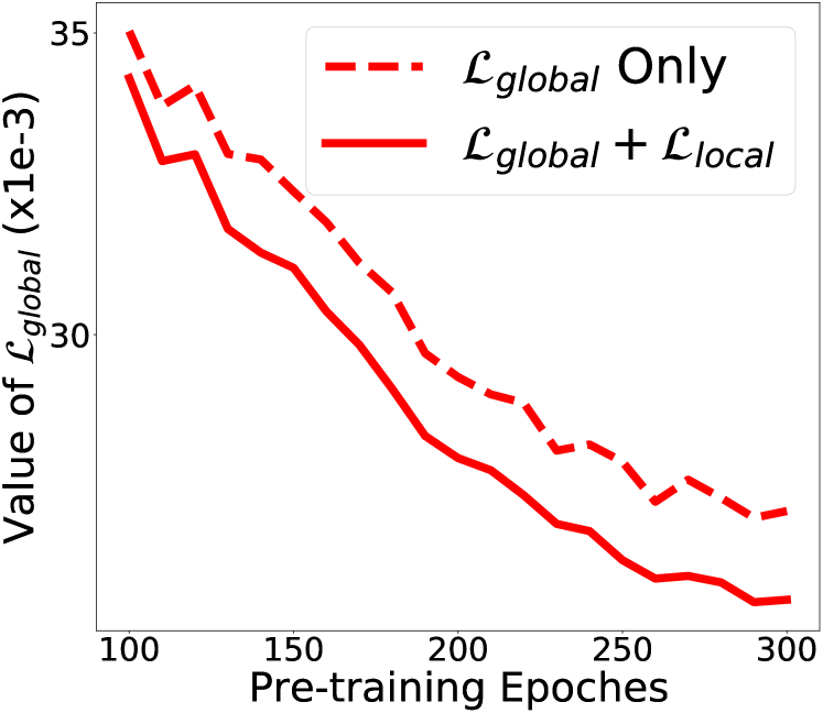
(a) $\mathcal{L}_{global}$

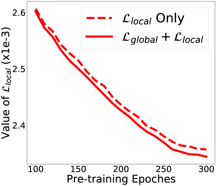
(b) $\mathcal{L}_{local}$

Figure 4: Loss curves of (a) $\mathcal{L}_{global}$ and (b) $\mathcal{L}_{local}$ with different learning objectives.

Decoder Architectures. While different encoder backbones have been investigated in existing works [10, 8], there are fewer studies on decoder architectures for the reconstruction-based SSL framework. Here we study the fully-connected decoder [57, 58] and the folding-based decoder [59], which are described in Sec. III-B, with Point-DAE framework. As illustrated in Fig. 8, although the reconstruction of a complete point cloud can be achieved with the DGCNN backbone, it only reconstructs the rough global shape due to the challenging corruptions. As can be seen in Tab. XI, the fully-connected decoder shows advantages on global shape reconstruction, which can be validated by comparing B1&B2, B3&B5, and B4&B6. On the contrary, the folding-based decoder is good at local patch reconstruction, as verified by the comparisons between B3&B4, and B5&B6. These findings echo the observations that the fully-connected decoder is good at capturing the global shape geometry, while the folding-based decoder is good at characterizing a smooth local surface [58].

TABLE XI: Results (%) with different decoder architectures.

	DGCNN Backbone
	Complete Point Cloud Decoder		Acc. (%)
B1	Folding-based		80.0
B2	Fully-connected		85.5
	Transformer Backbone
	Global Shape Decoder	Local Patch Decoder	Acc(%)
B3	Folding-based	Fully-connected	79.0
B4	Folding-based	Folding-based	81.2
B5	Fully-connected	Fully-connected	83.8
B6	Fully-connected	Folding-based	84.6

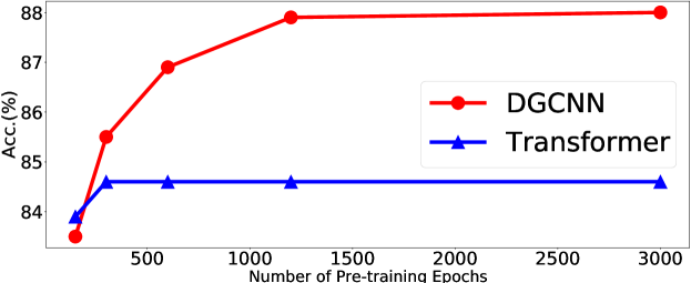
Figure 5: Results (%) with different number of pre-training epochs.

Masking Variants. Three masking strategies are compared in Tab. XII with only masking corruption. In the ‘View’ setting, points occluded in a random camera view are masked [10]. We mask fixed-sized KNN clusters and random-sized KNN clusters in the ‘Fixed-sized’ and ‘Random-sized’ settings, as detailed in Sec. III-C and Sec. III-B, respectively. The ‘Random-sized’ setting presents a clear advantage with the DGCNN backbone. However, this setting is incompatible with the Transformer backbones, where input patches are ‘Fixed-sized’ point clusters.

TABLE XII: Results (%) with different local masking methods.

Masking	View [10]	Fixed-sized [8]	Random-sized
Acc (%)	78.9	79.5	81.3

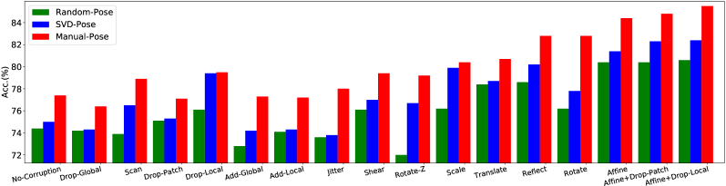
Figure 6: Results of Point-DAE with different pre-training datasets with and without manual poses. Experiments are conducted on the ObjBG setting of ScanObjectNN dataset under the linear classification protocol with the DGCNN backbone.

Impact of Transformation Module. As shown in Tab. XIII, the transformation module (i.e., T-Net) in PointNet [53] is incompatible with the affine transformation corruption. This fact may come from the intrinsic transformation rectification mechanism in T-Net, which dilutes the influence of affine transformation. We adopt the PointNet w/o T-Net as the default PointNet implementation. Although our adopted PointNet uses fewer parameters, it still significantly outperforms other competitors, as shown in Sec. IV-C.

TABLE XIII: Linear probing results of Point-DAE on the ObjBG setting of ScanObjectNN dataset, where only the affine transformation corruption is applied.

Methods	#Params	Acc. (%)
PointNet with T-Net	3.5M	73.8
PointNet w/o T-Net (our adopted)	0.8M	77.4

Pre-training epochs. As shown in Fig. 5, Point-DAE with Transformer backbone converges faster than that with DGCNN. In this work, we set the number of pre-training epochs as 300 in all experiments except those with DGCNN in Sec. IV-C, where we pre-train the model for $1,200$ epochs.

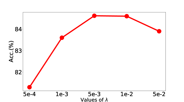
Figure 7: Results (%) with different values of $\lambda$.

Hyper-parameter $\lambda$. Results with different values of $\lambda$ are presented in Fig. 7. We empirically set $\lambda$ = 0.005 by default.

Corruption vs. Augmentation. We utilize the affine transformation as a simple data augmentation of masked modeling by modifying the reconstruction target $\mathbf{X}$ in Eq. (1) as the affine transformed $\mathrm{Affine}(\mathbf{X})$, leading to serious performance degeneration as shown in Tab. XIV. This reveals that the benefits of introduced affine transformation mainly come from the implicit instance discrimination principle [83, 3, 4], where each sample is treated as an individual category and affine transformed views of the same sample should perform similarly in the reconstruction.

TABLE XIV: Results (%) with different roles of affine transformation.

Roles of Affine Transformation	DGCNN	Transformer
Augmentation	81.8	83.0
Corruption	85.5	84.6

Object Poses of Pre-training Data. We also reveal that object poses of pre-training data play important roles in self-supervised point cloud learning, which is less investigated in the community. More specifically, samples are manually aligned to category-wise canonical poses in the popular pre-training datasets such as ShapeNet [60] and ModelNet [74]. In other words, the canonical poses implicitly carry the manual category annotation, which is unintentionally utilized by the SSL algorithms, including the vanilla auto-encoder, masked modeling and Point-DAE, as shown in Fig. 6. This does not conform to the practical scenarios where an unlabeled sample should not be manually assigned with any category-aware canonical pose.

One intuitive solution to overcome the dataset limitation is assigning each point cloud with a random pose, leading to the ‘Random-Pose’ setting. However, object pose plays an essential role in point cloud understanding [84, 85] and it should not be neglected. To make appropriate use of the pose information, we promote to automatically estimate the canonical pose for each sample with the singular value decomposition (SVD) strategy [86, 84], resulting in the ‘SVD-Pose’ setting, where poses of samples in the same category are roughly aligned without any manual effort. In contrast, the vanilla dataset with manual poses is termed as ‘Manual-Pose’.

As illustrated in Fig. 6, results with both ‘Manual-Pose’ and ‘SVD-Pose’ training data significantly outperform that with ‘Random-Pose’ data, demonstrating the importance of object poses in the pre-training dataset. Although the ‘Manual-Pose’ dataset has been widely used by the community and produces the best results, we recommend the ‘SVD-Pose’ setting for practical consideration, where the object poses are properly used without any manual effort. Viewed from the perspective of sample corruptions, the effectiveness of masking and affine transformation corruptions still holds under all the three dataset settings. Additionally, in all the three settings, combining masking and affine transformation corruptions leads to improved results over individual corruption, validating their complementary.

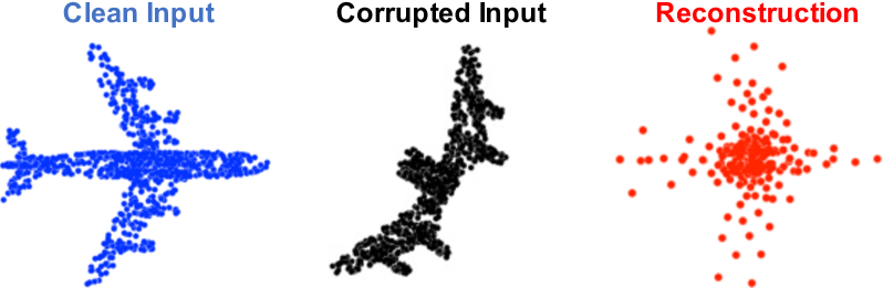
(a) DGCNN

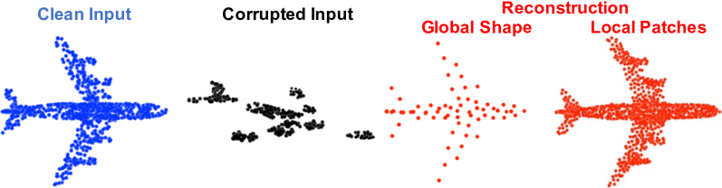
(b) Transformer

Figure 8: Visualization of reconstruction on ShapeNet validation set with backbones of DGCNN and Transformer. More visualization results and discussions can be found in the Supplementary Material.

Visualization. As illustrated in Fig. 8, the overall shape is reconstructed while the local details are hardly captured with the DGCNN backbone, due to the serious input corruptions of masking and affine transformation. For results with the Transformer backbone, both the global shape and local patches are well constructed, thanks to the decomposition of the construction objective.

Time complexity. All Point-DAE variants with the same encoder backbone share almost the same training and test complexity, since they are only different in the used corruptions, which could be conducted within the dataloader in a parallel manner.

V Conclusion

We comprehensively investigated the Point-DAE framework with $14$ corruption types. Besides the popular masking corruption, we identified another effective corruption family, i.e., affine transformation, which disturbed all points globally and is complementary to the local masking strategy. We validated the effectiveness of affine transformation corruption with various encoder backbones, including the traditional non-Transformer and the recent Transformer encoders. Especially, to alleviate the position leakage problem with the Transformer encoder, we decomposed the reconstruction of the complete point cloud into the reconstructions of detailed local patches and rough global shape, facilitating the pre-training efficacy. We validated the effectiveness of our method with various encoder backbones, under different evaluation protocols, and on extensive downstream point cloud tasks. In future work, we will explore the generality of affine transformation corruption with more data modalities, e.g., 2D images and videos, under the denoising autoencoder framework.

References

- [1] M. Noroozi and P. Favaro, “Unsupervised learning of visual representations by solving jigsaw puzzles,” in European conference on computer vision. Springer, 2016, pp. 69–84.
- [2] J. Sauder and B. Sievers, “Self-supervised deep learning on point clouds by reconstructing space,” Advances in Neural Information Processing Systems, vol. 32, 2019.
- [3] T. Chen, S. Kornblith, M. Norouzi, and G. Hinton, “A simple framework for contrastive learning of visual representations,” in International conference on machine learning. PMLR, 2020, pp. 1597–1607.
- [4] K. He, H. Fan, Y. Wu, S. Xie, and R. Girshick, “Momentum contrast for unsupervised visual representation learning,” in Proceedings of the IEEE/CVF conference on computer vision and pattern recognition, 2020, pp. 9729–9738.
- [5] A. Sanghi, “Info3d: Representation learning on 3d objects using mutual information maximization and contrastive learning,” in European Conference on Computer Vision. Springer, 2020, pp. 626–642.
- [6] K. He, X. Chen, S. Xie, Y. Li, P. Dollár, and R. Girshick, “Masked autoencoders are scalable vision learners,” arXiv preprint arXiv:2111.06377, 2021.
- [7] X. Yu, L. Tang, Y. Rao, T. Huang, J. Zhou, and J. Lu, “Point-bert: Pre-training 3d point cloud transformers with masked point modeling,” arXiv preprint arXiv:2111.14819, 2021.
- [8] Y. Pang, W. Wang, F. E. Tay, W. Liu, Y. Tian, and L. Yuan, “Masked autoencoders for point cloud self-supervised learning,” ECCV, 2022.
- [9] Z. Tong, Y. Song, J. Wang, and L. Wang, “Videomae: Masked autoencoders are data-efficient learners for self-supervised video pre-training,” arXiv preprint arXiv:2203.12602, 2022.
- [10] H. Wang, Q. Liu, X. Yue, J. Lasenby, and M. J. Kusner, “Unsupervised point cloud pre-training via occlusion completion,” in Proceedings of the IEEE/CVF International Conference on Computer Vision, 2021, pp. 9782–9792.
- [11] R. Zhang, Z. Guo, P. Gao, R. Fang, B. Zhao, D. Wang, Y. Qiao, and H. Li, “Point-m2ae: Multi-scale masked autoencoders for hierarchical point cloud pre-training,” arXiv preprint arXiv:2205.14401, 2022.
- [12] H. Liu, M. Cai, and Y. J. Lee, “Masked discrimination for self-supervised learning on point clouds,” arXiv preprint arXiv:2203.11183, 2022.
- [13] Y. Zhang, J. Lin, C. He, Y. Chen, K. Jia, and L. Zhang, “Masked surfel prediction for self-supervised point cloud learning,” arXiv preprint arXiv:2207.03111, 2022.
- [14] P. Vincent, H. Larochelle, Y. Bengio, and P.-A. Manzagol, “Extracting and composing robust features with denoising autoencoders,” in Proceedings of the 25th international conference on Machine learning, 2008, pp. 1096–1103.
- [15] M. Afham, I. Dissanayake, D. Dissanayake, A. Dharmasiri, K. Thilakarathna, and R. Rodrigo, “Crosspoint: Self-supervised cross-modal contrastive learning for 3d point cloud understanding,” arXiv preprint arXiv:2203.00680, 2022.
- [16] G. E. Hinton and R. R. Salakhutdinov, “Reducing the dimensionality of data with neural networks,” science, vol. 313, no. 5786, pp. 504–507, 2006.
- [17] A. Radford, K. Narasimhan, T. Salimans, I. Sutskever et al., “Improving language understanding by generative pre-training,” 2018.
- [18] J. Devlin, M.-W. Chang, K. Lee, and K. Toutanova, “Bert: Pre-training of deep bidirectional transformers for language understanding,” arXiv preprint arXiv:1810.04805, 2018.
- [19] H. Bao, L. Dong, S. Piao, and F. Wei, “Beit: Bert pre-training of image transformers,” arXiv preprint arXiv:2106.08254, 2021.
- [20] C. Feichtenhofer, H. Fan, Y. Li, and K. He, “Masked autoencoders as spatiotemporal learners,” arXiv preprint arXiv:2205.09113, 2022.
- [21] A. Vaswani, N. Shazeer, N. Parmar, J. Uszkoreit, L. Jones, A. N. Gomez, Ł. Kaiser, and I. Polosukhin, “Attention is all you need,” Advances in neural information processing systems, vol. 30, 2017.
- [22] J. T. Rolfe, “Discrete variational autoencoders,” arXiv preprint arXiv:1609.02200, 2016.
- [23] S. Yan, Z. Yang, H. Li, L. Guan, H. Kang, G. Hua, and Q. Huang, “Implicit autoencoder for point cloud self-supervised representation learning,” arXiv preprint arXiv:2201.00785, 2022.
- [24] Y. Li, R. Bu, M. Sun, W. Wu, X. Di, and B. Chen, “Pointcnn: Convolution on x-transformed points,” Advances in neural information processing systems, vol. 31, 2018.
- [25] H. Thomas, C. R. Qi, J.-E. Deschaud, B. Marcotegui, F. Goulette, and L. J. Guibas, “Kpconv: Flexible and deformable convolution for point clouds,” in Proceedings of the IEEE/CVF international conference on computer vision, 2019, pp. 6411–6420.
- [26] W. Wu, Z. Qi, and L. Fuxin, “Pointconv: Deep convolutional networks on 3d point clouds,” in Proceedings of the IEEE/CVF Conference on computer vision and pattern recognition, 2019, pp. 9621–9630.
- [27] S. Qiu, S. Anwar, and N. Barnes, “Dense-resolution network for point cloud classification and segmentation,” in Proceedings of the IEEE/CVF Winter Conference on Applications of Computer Vision, 2021, pp. 3813–3822.
- [28] H. Zhao, L. Jiang, J. Jia, P. H. Torr, and V. Koltun, “Point transformer,” in Proceedings of the IEEE/CVF International Conference on Computer Vision, 2021, pp. 16 259–16 268.
- [29] X. Ma, C. Qin, H. You, H. Ran, and Y. Fu, “Rethinking network design and local geometry in point cloud: A simple residual mlp framework,” arXiv preprint arXiv:2202.07123, 2022.
- [30] Z. Liu, H. Hu, Y. Cao, Z. Zhang, and X. Tong, “A closer look at local aggregation operators in point cloud analysis,” in Computer Vision–ECCV 2020: 16th European Conference, Glasgow, UK, August 23–28, 2020, Proceedings, Part XXIII 16. Springer, 2020, pp. 326–342.
- [31] X. Wu, Y. Lao, L. Jiang, X. Liu, and H. Zhao, “Point transformer v2: Grouped vector attention and partition-based pooling,” arXiv preprint arXiv:2210.05666, 2022.
- [32] M. Xu, R. Ding, H. Zhao, and X. Qi, “Paconv: Position adaptive convolution with dynamic kernel assembling on point clouds,” in Proceedings of the IEEE/CVF Conference on Computer Vision and Pattern Recognition, 2021, pp. 3173–3182.
- [33] G. Qian, Y. Li, H. Peng, J. Mai, H. A. A. K. Hammoud, M. Elhoseiny, and B. Ghanem, “Pointnext: Revisiting pointnet++ with improved training and scaling strategies,” arXiv preprint arXiv:2206.04670, 2022.
- [34] M.-H. Guo, J.-X. Cai, Z.-N. Liu, T.-J. Mu, R. R. Martin, and S.-M. Hu, “Pct: Point cloud transformer,” Computational Visual Media, vol. 7, no. 2, pp. 187–199, 2021.
- [35] T. Xiang, C. Zhang, Y. Song, J. Yu, and W. Cai, “Walk in the cloud: Learning curves for point clouds shape analysis,” in Proceedings of the IEEE/CVF International Conference on Computer Vision, 2021, pp. 915–924.
- [36] O. Poursaeed, T. Jiang, H. Qiao, N. Xu, and V. G. Kim, “Self-supervised learning of point clouds via orientation estimation,” in 2020 International Conference on 3D Vision (3DV). IEEE, 2020, pp. 1018–1028.
- [37] Z. Zhang, R. Girdhar, A. Joulin, and I. Misra, “Self-supervised pretraining of 3d features on any point-cloud,” in Proceedings of the IEEE/CVF International Conference on Computer Vision, 2021, pp. 10 252–10 263.
- [38] S. Xie, J. Gu, D. Guo, C. R. Qi, L. Guibas, and O. Litany, “Pointcontrast: Unsupervised pre-training for 3d point cloud understanding,” in European conference on computer vision. Springer, 2020, pp. 574–591.
- [39] Y. Rao, J. Lu, and J. Zhou, “Global-local bidirectional reasoning for unsupervised representation learning of 3d point clouds,” in Proceedings of the IEEE/CVF Conference on Computer Vision and Pattern Recognition, 2020, pp. 5376–5385.
- [40] R. Zhang, L. Wang, Y. Qiao, P. Gao, and H. Li, “Learning 3d representations from 2d pre-trained models via image-to-point masked autoencoders,” in Proceedings of the IEEE/CVF Conference on Computer Vision and Pattern Recognition, 2023, pp. 21 769–21 780.
- [41] Z. Qi, R. Dong, G. Fan, Z. Ge, X. Zhang, K. Ma, and L. Yi, “Contrast with reconstruct: Contrastive 3d representation learning guided by generative pretraining,” arXiv preprint arXiv:2302.02318, 2023.
- [42] Y. Chen, J. Liu, B. Ni, H. Wang, J. Yang, N. Liu, T. Li, and Q. Tian, “Shape self-correction for unsupervised point cloud understanding,” in Proceedings of the IEEE/CVF International Conference on Computer Vision, 2021, pp. 8382–8391.
- [43] M. Xu, Z. Zhou, H. Xu, Y. Wang, and Y. Qiao, “Cp-net: Contour-perturbed reconstruction network for self-supervised point cloud learning,” arXiv preprint arXiv:2201.08215, 2022.
- [44] E. D. Cubuk, B. Zoph, D. Mane, V. Vasudevan, and Q. V. Le, “Autoaugment: Learning augmentation strategies from data,” in Proceedings of the IEEE/CVF Conference on Computer Vision and Pattern Recognition, 2019, pp. 113–123.
- [45] E. D. Cubuk, B. Zoph, J. Shlens, and Q. V. Le, “Randaugment: Practical automated data augmentation with a reduced search space,” in Proceedings of the IEEE/CVF conference on computer vision and pattern recognition workshops, 2020, pp. 702–703.
- [46] D. Hendrycks, N. Mu, E. D. Cubuk, B. Zoph, J. Gilmer, and B. Lakshminarayanan, “Augmix: A simple data processing method to improve robustness and uncertainty,” arXiv preprint arXiv:1912.02781, 2019.
- [47] D. Hendrycks and T. Dietterich, “Benchmarking neural network robustness to common corruptions and perturbations,” arXiv preprint arXiv:1903.12261, 2019.
- [48] J. Ren, L. Pan, and Z. Liu, “Benchmarking and analyzing point cloud classification under corruptions,” International Conference on Machine Learning (ICML), 2022.
- [49] K. Sohn, D. Berthelot, N. Carlini, Z. Zhang, H. Zhang, C. A. Raffel, E. D. Cubuk, A. Kurakin, and C.-L. Li, “Fixmatch: Simplifying semi-supervised learning with consistency and confidence,” Advances in neural information processing systems, vol. 33, pp. 596–608, 2020.
- [50] C. Dong, C. C. Loy, K. He, and X. Tang, “Image super-resolution using deep convolutional networks,” IEEE transactions on pattern analysis and machine intelligence, vol. 38, no. 2, pp. 295–307, 2015.
- [51] L. Yu, X. Li, C.-W. Fu, D. Cohen-Or, and P.-A. Heng, “Pu-net: Point cloud upsampling network,” in Proceedings of the IEEE conference on computer vision and pattern recognition, 2018, pp. 2790–2799.
- [52] H. Fan, H. Su, and L. J. Guibas, “A point set generation network for 3d object reconstruction from a single image,” in Proceedings of the IEEE conference on computer vision and pattern recognition, 2017, pp. 605–613.
- [53] C. R. Qi, H. Su, K. Mo, and L. J. Guibas, “Pointnet: Deep learning on point sets for 3d classification and segmentation,” in Proceedings of the IEEE conference on computer vision and pattern recognition, 2017, pp. 652–660.
- [54] C. R. Qi, L. Yi, H. Su, and L. J. Guibas, “Pointnet++: Deep hierarchical feature learning on point sets in a metric space,” Advances in neural information processing systems, vol. 30, 2017.
- [55] Y. Wang, Y. Sun, Z. Liu, S. E. Sarma, M. M. Bronstein, and J. M. Solomon, “Dynamic graph cnn for learning on point clouds,” Acm Transactions On Graphics (tog), vol. 38, no. 5, pp. 1–12, 2019.
- [56] J. Sun, Q. Zhang, B. Kailkhura, Z. Yu, C. Xiao, and Z. M. Mao, “Benchmarking robustness of 3d point cloud recognition against common corruptions,” arXiv preprint arXiv:2201.12296, 2022.
- [57] P. Achlioptas, O. Diamanti, I. Mitliagkas, and L. Guibas, “Learning representations and generative models for 3d point clouds,” in International conference on machine learning. PMLR, 2018, pp. 40–49.
- [58] W. Yuan, T. Khot, D. Held, C. Mertz, and M. Hebert, “Pcn: Point completion network,” in 2018 International Conference on 3D Vision (3DV). IEEE, 2018, pp. 728–737.
- [59] Y. Yang, C. Feng, Y. Shen, and D. Tian, “Foldingnet: Point cloud auto-encoder via deep grid deformation,” in Proceedings of the IEEE conference on computer vision and pattern recognition, 2018, pp. 206–215.
- [60] A. X. Chang, T. Funkhouser, L. Guibas, P. Hanrahan, Q. Huang, Z. Li, S. Savarese, M. Savva, S. Song, H. Su, J. Xiao, L. Yi, and F. Yu, “ShapeNet: An Information-Rich 3D Model Repository,” Stanford University — Princeton University — Toyota Technological Institute at Chicago, Tech. Rep. arXiv:1512.03012 [cs.GR], 2015.
- [61] A. Dai, A. X. Chang, M. Savva, M. Halber, T. Funkhouser, and M. Nießner, “Scannet: Richly-annotated 3d reconstructions of indoor scenes,” in Proceedings of the IEEE conference on computer vision and pattern recognition, 2017, pp. 5828–5839.
- [62] I. Loshchilov and F. Hutter, “Decoupled weight decay regularization,” arXiv preprint arXiv:1711.05101, 2017.
- [63] ——, “Sgdr: Stochastic gradient descent with warm restarts,” arXiv preprint arXiv:1608.03983, 2016.
- [64] B. Du, X. Gao, W. Hu, and X. Li, “Self-contrastive learning with hard negative sampling for self-supervised point cloud learning,” in Proceedings of the 29th ACM International Conference on Multimedia, 2021, pp. 3133–3142.
- [65] S. Huang, Y. Xie, S.-C. Zhu, and Y. Zhu, “Spatio-temporal self-supervised representation learning for 3d point clouds,” in Proceedings of the IEEE/CVF International Conference on Computer Vision, 2021, pp. 6535–6545.
- [66] Q. Zhang and J. Hou, “Self-supervised pre-training for 3d point clouds via view-specific point-to-image translation,” arXiv preprint arXiv:2212.14197, 2022.
- [67] Y. Liu, X. Yan, Z. Chen, Z. Li, Z. Wei, and M. Wei, “Pointgame: Geometrically and adaptively masked auto-encoder on point clouds,” arXiv preprint arXiv:2303.13100, 2023.
- [68] M. Szachniewicz, W. Kozłowski, M. Stypułkowski, and M. Zikeba, “Self-supervised adversarial masking for 3d point cloud representation learning,” arXiv preprint arXiv:2307.05325, 2023.
- [69] Z. Wang, X. Yu, Y. Rao, J. Zhou, and J. Lu, “Take-a-photo: 3d-to-2d generative pre-training of point cloud models,” arXiv preprint arXiv:2307.14971, 2023.
- [70] Z. Guo, X. Li, and P. A. Heng, “Joint-mae: 2d-3d joint masked autoencoders for 3d point cloud pre-training,” arXiv preprint arXiv:2302.14007, 2023.
- [71] J. Jiang, X. Lu, L. Zhao, R. Dazeley, and M. Wang, “Masked autoencoders in 3d point cloud representation learning,” arXiv preprint arXiv:2207.01545, 2022.
- [72] K. A. Zeid, J. Schult, A. Hermans, and B. Leibe, “Point2vec for self-supervised representation learning on point clouds,” arXiv preprint arXiv:2303.16570, 2023.
- [73] R. Dong, Z. Qi, L. Zhang, J. Zhang, J. Sun, Z. Ge, L. Yi, and K. Ma, “Autoencoders as cross-modal teachers: Can pretrained 2d image transformers help 3d representation learning?” arXiv preprint arXiv:2212.08320, 2022.
- [74] Z. Wu, S. Song, A. Khosla, F. Yu, L. Zhang, X. Tang, and J. Xiao, “3d shapenets: A deep representation for volumetric shapes,” in Proceedings of the IEEE conference on computer vision and pattern recognition, 2015, pp. 1912–1920.
- [75] M. A. Uy, Q.-H. Pham, B.-S. Hua, T. Nguyen, and S.-K. Yeung, “Revisiting point cloud classification: A new benchmark dataset and classification model on real-world data,” in Proceedings of the IEEE/CVF international conference on computer vision, 2019, pp. 1588–1597.
- [76] J. Ren, L. Pan, and Z. Liu, “Benchmarking and analyzing point cloud classification under corruptions,” arXiv preprint arXiv:2202.03377, 2022.
- [77] A. Poulenard, M.-J. Rakotosaona, Y. Ponty, and M. Ovsjanikov, “Effective rotation-invariant point cnn with spherical harmonics kernels,” in 2019 International Conference on 3D Vision (3DV). IEEE, 2019, pp. 47–56.
- [78] Y. Rao, J. Lu, and J. Zhou, “Spherical fractal convolutional neural networks for point cloud recognition,” in Proceedings of the IEEE/CVF Conference on Computer Vision and Pattern Recognition, 2019, pp. 452–460.
- [79] S. Kim, J. Park, and B. Han, “Rotation-invariant local-to-global representation learning for 3d point cloud,” Advances in Neural Information Processing Systems, vol. 33, pp. 8174–8185, 2020.
- [80] C. R. Qi, O. Litany, K. He, and L. J. Guibas, “Deep hough voting for 3d object detection in point clouds,” in proceedings of the IEEE/CVF International Conference on Computer Vision, 2019, pp. 9277–9286.
- [81] I. Misra, R. Girdhar, and A. Joulin, “An end-to-end transformer model for 3d object detection,” in Proceedings of the IEEE/CVF International Conference on Computer Vision, 2021, pp. 2906–2917.
- [82] C. Sharma and M. Kaul, “Self-supervised few-shot learning on point clouds,” Advances in Neural Information Processing Systems, vol. 33, pp. 7212–7221, 2020.
- [83] Z. Wu, Y. Xiong, S. X. Yu, and D. Lin, “Unsupervised feature learning via non-parametric instance discrimination,” in Proceedings of the IEEE conference on computer vision and pattern recognition, 2018, pp. 3733–3742.
- [84] C. Zhao, J. Yang, X. Xiong, A. Zhu, Z. Cao, and X. Li, “Rotation invariant point cloud analysis: Where local geometry meets global topology,” Pattern Recognition, vol. 127, p. 108626, 2022.
- [85] F. Li, K. Fujiwara, F. Okura, and Y. Matsushita, “A closer look at rotation-invariant deep point cloud analysis,” in Proceedings of the IEEE/CVF International Conference on Computer Vision, 2021, pp. 16 218–16 227.
- [86] G. H. Golub and C. Reinsch, “Singular value decomposition and least squares solutions,” in Linear algebra. Springer, 1971, pp. 134–151.