Deterministic Interrelation Between Elastic Moduli in Critically Elastic Materials

Abstract

Critically elastic materials – those that are rigid with a single state of self-stress – can be generated from parent systems with two states of self-stress by the removal of one of many constraints. We show that the elastic moduli of the resulting homogeneous and isotropic daughter systems are interrelated by a universal functional form parametrized by properties of the parent. In simulations of both spring networks and packings of soft spheres, judicious choice of parent systems and bond removal allows for the selection of a wide variety of moduli and Poisson’s ratios in the critically elastic systems, providing a framework for versatile deterministic selection of mechanical properties.

Disordered materials of homogeneous and isotropic structure are known to have exactly two independent linear elastic constants, expressible as a bulk modulus and a shear modulus Hodge (1961); Jog (2006); Gould and Feng (1994); Slaughter (2012). On the microscopic structural level, the rigidity and linear mechanical response of a disordered composite system, such as a packing of soft particles, can be described by the deformational response of an underlying elastic network, with each bond representing the interaction of two touching particles. A soft network with $N$ nodes and $N_{c}$ elastic bonds (often represented by springs) is minimally rigid (isostatic) if the number of constraining bonds $N_{c}$ exactly balances the number of degrees of freedom ($Nd$ in $d$ dimensions) Maxwell (1864); Calladine (1978). However, an isostatic system is not able to sustain generic stress due to its vanishing shear modulus  Ellenbroek et al. (2009); Wyart et al. (2008); Zaccone and Scossa-Romano (2011); Zaccone et al. (2011); Ellenbroek et al. (2015). For a network to be able to carry a force, it needs to have at least one state of self-stress, defined as modes of putting load on the local constraints (contacts in jamming and springs in the elastic network model) while keeping the entire system at mechanical equilibrium.

Here, we focus on critically elastic systems – those that are rigid and support exactly one state of self-stress (SSS). We show that there is a deterministic functional dependence between the bulk and shear moduli of the critically elastic systems regardless of their preparation protocol, and that understanding this relation allows for the informed selection of a great variety of mechanical behaviors when these systems are generated from parents with two states of self-stress by removal of a single constraint. Fig. 1 illustrates this core finding in two spring network samples.

Figure 1: (a, b) Two parent spring networks with $m=2$ states of self-stress produced by randomly removing stressed bonds from a Delaunay triangulation while imposing Hilbert’s stability condition on each node. (c, d) Values of the normalized bulk ($K^{\prime}/K$) versus shear ($G^{\prime}/G$) modulus after removing a single bond from networks in (a) and (b) respectively. The $m=2\rightarrow 1$ nomenclature indicates that the elastic moduli are calculated for the daughter networks generated by removing a random constraint from the parent network. Each black data point corresponds to one daughter network thus generated. Both networks have similar structures but different correlations between the normalized moduli. The blue ellipses are drawn using Eq. 7.

States of self-stress are described by a set of orthogonal $N_{c}\times 1$ vectors, $\{\mathbf{s}_{i}\}$, where the entries of each vector are the tensions in individual bonds. Without loss of generality, we will normalize these vectors to unit length. When a spring network with $m$ states of self-stress is deformed, the stored elastic energy is obtained from the projection of the deformation vector, $\bm{\Delta}$, onto the states of self-stress Lubensky et al. (2015); Hexner et al. (2018); Paulose et al. (2015):

$$\delta E=\frac{1}{2}\sum_{i=1}^{m}(\mathbf{s}_{i}.\bm{\Delta})^{2}.$$ (1)

where $\bm{\Delta}$ is the $N_{c}\times 1$ vector of changes in the individual spring lengths from their rest lengths.

All continuum mechanical behavior of a homogeneous and isotropic network can be obtained from two types of probing strains, often chosen as isotropic compressional strain, $\bm{\epsilon}_{+}$, and shear strain, $\bm{\epsilon}_{-}$. Here, we restrict ourselves to the $2D$ case where $(\bm{\epsilon}_{+})_{IJ}=\epsilon_{+}\delta_{IJ}$, and $(\bm{\epsilon}_{-})_{IJ}=(-1)^{I+1}\epsilon_{-}\delta_{IJ}$ with $I,J=\{1,2\}$. However, the results presented are valid for any generic form of strain in $d$ dimensions, independent of the imposed boundary conditions. After obtaining the respective deformations $\bm{\Delta}_{+}$ and $\bm{\Delta}_{-}$ and their corresponding deformation energies, $\delta E_{+},\delta E_{-}$, one can infer the elastic bulk and shear moduli, $K=\frac{\delta E}{2V\epsilon_{+}^{2}}$ and $G=\frac{\delta E}{2V\epsilon_{-}^{2}}$, where $V$ is the volume of the system. In the linear elastic limit, the modulus values are independent of $\epsilon_{+},\epsilon_{-}$ Gould and Feng (1994); Slaughter (2012); Hagh (2018); Hagh and Sadjadi (2022). See Appendix A for a more thorough discussion.

Removing constraints from an elastic network structure changes its moduli, which is key in many material design algorithms. For instance, in tuning by pruning, one can tune a single elastic modulus (or the ratio of the two independent elastic moduli) in a predictable way by selective removal of constraints in multiple steps Goodrich et al. (2015); Hagh and Thorpe (2018); Reid et al. (2018); Hagh et al. (2019); Hexner et al. (2018). When a system is far from marginal rigidity, meaning that there are more constraints than degrees of freedom, $N_{c}\gg Nd$, removing a single constraint typically does not change the elastic moduli significantly. Closer to the onset of rigidity, however, single constraint alterations can change the elastic moduli much more effectively, and as we show below, it reduces the number of independent elastic constants to one in going from $m=2\to 1$ SSS.

Note that in packings or networks with multiple states of self-stress, any superposition of these states is also a valid self-stress. In addition, removing any of the constraining bonds in areas of a parent network where stress percolates (we call these stressed or load-bearing bonds as they will undergo stress if the network is deformed) removes one state of self-stress, transitioning the network from, say, $m$ SSS and $N_{c}$ bonds to a new daughter network with $(m-1)$ SSS and $N_{c}-1$ bonds ($m\rightarrow m-1$). Instead of writing the daughter network’s states of self-stress as vectors of dimension $N_{c}-1$, we can write them as $N_{c}$-dimensional vectors with a zero entry at the position of the removed bond in the parent network. This can be done at any given number of constraints above isostaticity. The states of self-stress in the daughter system (denoted by primed vectors) can thus be written as a linear combination of the states of self-stress in the parent system, i.e.

$$\mathbf{s}^{\prime}_{j}=\sum_{i=1}^{m}\alpha_{ij}\mathbf{s}_{i}\,$$ (2)

where $\alpha_{ij}$ represent $m(m-1)$ coefficients. However, not all $\alpha_{ij}$ are independent. Consistent with the treatment of $\mathbf{s}_{i}$ in the parent network, the states of self-stress in the daughter network are again orthonormal ($\mathbf{s}^{\prime}_{i}\cdot\mathbf{s}^{\prime}_{j}=\delta_{ij}$). This adds $m(m-1)/2$ constraints to the set of new states of self-stress. Furthermore, the tension on the removed bond (say, bond $l$) is required to be zero ($s^{\prime}_{j,l}=0$), which leaves the set of self-stresses with another $m-1$ constraints. Thus, the total number of independent free parameters, $\alpha_{ij}$, is $(m-1)(m-2)/2$. While for large $m$ there are $\mathcal{O}(m^{2})$ free parameters, neither of the $m=2$ or $m=1$ cases have any free parameters left. The case of $m=1$ is rather trivial since the system has no remaining states of self-stress once a constraint is removed. The $m=2$ case is non-trivial and the focus of the current work. According to the above analysis, the two states of self-stress in the $m=2$ parent network uniquely determine the single state of self-stress in the daughter network after a single bond is removed.

Let $(\mathbf{s}_{1},\mathbf{s}_{2})$ be the states of self-stress of a $m=2$ parent network. Using Eq. 2, we can write the single self-stress of the daughter network, $\mathbf{s}^{\prime}$, as:

$$\mathbf{s}^{\prime}=\frac{\mathbf{s}_{1}+\chi_{l}\mathbf{s}_{2}}{\sqrt{1+\chi_{l}^{2}}}.$$ (3)

Note that $\mathbf{s^{\prime}}$ is normalized and $\chi_{l}$ must be chosen such that the tension on spring $l$ is zero, i.e. $s^{\prime}_{l}=0$. Thus $\chi_{l}=-{s_{1,l}}/{s_{2,l}}$ assuming $s_{2,l}\neq 0$ (without loss of generality, as for the bond $l$ at least one of $s_{1,l},s_{2,l}$ is non-zero). We drop the subscript $l$ in the following steps as $l$ can be any of the bonds in stressed regions in the parent system. We will now use (3) to write the moduli ($K^{\prime},G^{\prime}$) of the $m=1$ daughter network as functions of the $m=2$ parent network properties, $K,G$.

Eq. 1 with $\bm{\Delta}_{+}$ and $\bm{\Delta}_{-}$ corresponding to the deformations of the two elastic moduli yields, for the parent network:

$$K =\frac{1}{4}[\left(\mathbf{s}_{1}.\bm{\Delta}_{+}\right)^{2}+\left(\mathbf{s}_{2}.\bm{\Delta}_{+}\right)^{2}]=\frac{1}{4}(a_{1}^{2}+a_{2}^{2}),$$

$$G =\frac{1}{4}[\left(\mathbf{s}_{1}.\bm{\Delta}_{-}\right)^{2}+\left(\mathbf{s}_{2}.\bm{\Delta}_{-}\right)^{2}]=\frac{1}{4}(b_{1}^{2}+b_{2}^{2}),$$ (4)

where the second equalities in each equation define $a_{1}$, $a_{2}$, $b_{1}$, $b_{2}$. The analogous relations for the daughter network, together with Eq. 3, give the elastic moduli after removing a bond:

$$K^{\prime} =\frac{1}{4}(\mathbf{s}^{\prime}.\bm{\Delta}^{{}^{\prime}}_{+})^{2}=\frac{[\left(\mathbf{s}_{1}+\chi\mathbf{s}_{2}\right).\bm{\Delta}_{+}]^{2}}{4(1+\chi^{2})}=\frac{\left(a_{1}+\chi a_{2}\right)^{2}}{4(1+\chi^{2})},$$

$$G^{\prime} =\frac{1}{4}(\mathbf{s}^{\prime}.\bm{\Delta}^{{}^{\prime}}_{-})^{2}=\frac{[\left(\mathbf{s}_{1}+\chi\mathbf{s}_{2}\right).\bm{\Delta}_{-}]^{2}}{4(1+\chi^{2})}=\frac{\left(b_{1}+\chi b_{2}\right)^{2}}{4(1+\chi^{2})}.$$ (5)

Figure 2: Normalized elastic moduli, $(K^{\prime}/K,G^{\prime}/G)$ for $m=2\to 1$, $3\to 2$, $4\to 3$, $5\to 4$ and $m=12\to 11$ SSS in two sets of networks with $\left[\frac{\pi}{4}\right]$ (top) and $\left[-\frac{\pi}{4}\right]$ (bottom) orientations. For larger $m$, the networks exhibit more robust response to bond removal and changes in elastic moduli after removing a bond tend to be smaller, leading to the clustering of moduli values near upper right corner. However, closer to $m=1$, the elastic response can vary significantly by removing a single bond due to the criticality of the network. Although for $m=3\to 2$ the normalized elastic moduli are no longer on the perimeter of the characteristic ellipse, the signature of the ellipse is still present in the elastic response.

It is evident that $(K^{\prime},G^{\prime})$ are bounded by the values of elastic moduli in the parent network, i.e. $0\leq K^{\prime}\leq K$ and $0\leq G^{\prime}\leq G$. Therefore, it is useful to define the normalized elastic moduli $K^{\prime}/K,G^{\prime}/G$ as:

$$\frac{K^{\prime}}{K} =\frac{(a_{1}+\chi a_{2})^{2}}{(a_{1}^{2}+a_{2}^{2})(1+\chi^{2})},$$

$$\frac{G^{\prime}}{G} =\frac{(b_{1}+\chi b_{2})^{2}}{(b_{1}^{2}+b_{2}^{2})(1+\chi^{2})}.$$ (6)

These equations are the parameterization of an ellipse in terms of $\chi$ (see Appendix B for proof). This means the elastic moduli of the network with $m=1$ state of self-stress are not independent and are related through an elliptic equation which, in standard form, can be written as:

$$\left(\frac{\frac{K^{\prime}}{K}+\frac{G^{\prime}}{G}-1}{\sqrt{1-\eta}}\right)^{2}+\left(\frac{\frac{K^{\prime}}{K}-\frac{G^{\prime}}{G}}{\sqrt{\eta}}\right)^{2}=1,$$ (7)

where $\eta$ is:

$$\eta\equiv\frac{(a_{1}b_{2}-a_{2}b_{1})^{2}}{(b_{1}^{2}+b_{2}^{2})(a_{1}^{2}+a_{2}^{2})}.$$ (8)

In large systems with many available constraints, the distribution of $\chi$ covers a wide range of values and this parameterization puts all values of the moduli after removing a bond on the perimeter of an ellipse given by Eq. 7. Two examples are shown in Fig. 1, where the black data points on each ellipse correspond to the normalized elastic moduli of its corresponding parent network, $(K^{\prime}/K,G^{\prime}/G)$, after removing a random bond. Both networks in Fig. 1a,b are prepared using a selective pruning algorithm in which stressed bonds are removed randomly from a Delaunay triangulation Lee and Schachter (1980) while imposing Hilbert’s stability condition, requiring each node to have at least $d+1$ bonds, positioned such that any two adjacent bonds make an angle smaller than $\pi$ Alexander (1998); Lopez et al. (2013).

Note that $\eta$ is completely determined by the elastic response of the parent network at $m=2$ SSS and ranges from $0$ to $1$. Moreover, $\eta$ fully controls the shape of the ellipse. Eq. 7 is the equation of an ellipse with its center at (1/2, 1/2). When $\eta\in(0,1/2)$, the major axis of the ellipse is $\sqrt{1-\eta}$ and oriented along ${K^{\prime}}/{K}+{G^{\prime}}/{G}=1$ (under a $\left[-\frac{\pi}{4}\right]$ angle), while for $\eta\in(1/2,1)$, the major axis is $\sqrt{\eta}$ and oriented along ${K^{\prime}}/{K}-{G^{\prime}}/{G}=0$ (under a $\left[+\frac{\pi}{4}\right]$ angle). The ellipse becomes a circle for $\eta=1/2$ and asymptotes to a line for $\eta=0$ or $\eta=1$.

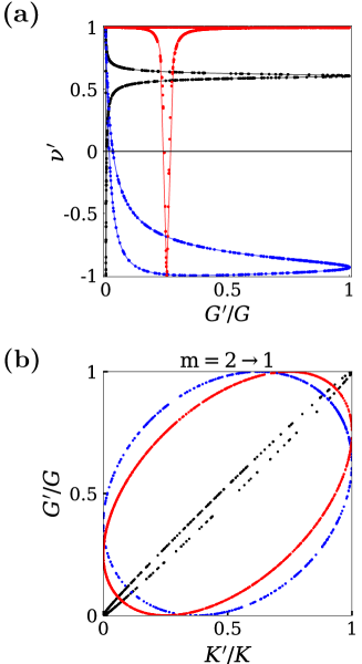
Figure 3: (a) Poisson’s ratio, $\nu^{\prime}$, of three networks each with $m=1$ SSS and various values of $\eta$: (black) a spring network generated by randomly removing stressed bonds from a Delaunay triangulation while imposing Hilbert’s stability condition on each node with $\eta\approx 0.001$, $G/K\approx 0.244$, and $\nu\approx 0.610$ in the parent network; (blue) an auxetic network with $\eta\approx 0.374$, and $G/K\approx 18.50$ and $\nu\approx-0.90$; (red) a jammed network with $\eta\approx 0.251$, $G/K\approx 0.0006$, and $\nu\approx 0.998$. The solid lines are drawn using Eq. 7 and Eq. 9 and data points are obtained by removing bonds and measuring the elastic moduli directly from the networks. In all three networks, there are bonds that change the sign of the Poisson’s ratio when removed. (b) The characteristic ellipses of the three networks shown in (a). Each color matches the color of its corresponding curve in (a).

The angle of the ellipse divides critically elastic systems into two classes (as demonstrated in Fig. 1). In the first class, identified with a $\left[+\frac{\pi}{4}\right]$ angle, elastic moduli change in a positively correlated fashion, i.e. the system is robust against removal of certain bonds (both bulk and shear moduli change very little), but very sensitive against the removal of others (both bulk and shear moduli are reduced dramatically).

The second class consists of those systems that produce a $\left[-\frac{\pi}{4}\right]$ angle ellipse. Here, changes in the bulk and shear modulus are negatively correlated: if removing a bonds changes the shear modulus drastically, it leaves the bulk modulus virtually unchanged and vice versa. These networks are suitable when one intends to change only one of the elastic moduli significantly.

Since $\eta$ is a function of both the constraint pattern and states of self-stress, its value and therefore the class to which the network belongs is ultimately a function of structural details such as the location of nodes or particles and the contact network. We have studied networks created with different protocols (jamming or selective pruning of bonds from a Delaunay triangulation) and observe that regardless of the used protocol, resulting networks can have a positively or negatively correlated elastic response. As the moduli are determined by global deformation energies (Eq. 1), these phenomena also persist independent of variations in particle sizes, spring constants, or boundary conditions.

The change in elastic moduli upon transitioning from $m=2$ to the critically elastic, $m=1$ state, shows qualitative differences to transitions at higher numbers of states of self-stress. Fig. 2 compares the normalized elastic moduli of the $m=2\to 1$ transition (which produces the ellipse) to transitions at larger $m\to m-1$ for two sets of networks. Starting with $m=12$ SSS, we sequentially remove constraints to reach lower numbers of SSS. We then use the resulting networks as the parent network for each panel presented in the figure. Although the details depend on the specifics of the network, we generally observe that the deterministic functional dependence between the bulk and shear moduli quickly disappears as we go to larger $m$. While the normalized moduli maintain some degree of elliptical signature when we go from $m=3\to 2$, this correlation is quickly lost for higher $m\to m-1$. It can also be seen from Fig. 2 that already for moderately large $m$, both $K^{\prime}/K$ and $G^{\prime}/G$ approach $1$ for most bond removals, which is intuitive as only exceptional bonds can significantly alter the mechanics of a network with many states of self-stress. Note, however, that for intermediate values such as $m=3,4$ the scattered outputs cover a greater area of the normalized moduli unit square, making these cases attractive if a wide variation of mechanical response is desired.

Since normalized elastic moduli form a closed curve, any horizontal or vertical line would cross the curve at exactly two points. This means when $N_{c}\rightarrow\infty$, for any given value of the bulk (shear) modulus, there are two bonds whose removal leads to different values for the shear (bulk) modulus, implying interrelated pairs of bonds. This effect can be best represented by the Poisson’s ratio, defined as:

$$\nu=\frac{dK-2G}{d(d-1)K+2G}$$ (9)

for a generic $d$ dimensional elastic system. Note that Poisson’s ratio is bounded by $-1<\nu<\frac{1}{d-1}$. For ordinary isotropic materials, Poisson’s ratio is always positive. For systems with $m=1$ SSS in $2D$, Eq. 9 reduces to:

$$\nu^{\prime}=\frac{K^{\prime}-G^{\prime}}{K^{\prime}+G^{\prime}}.$$ (10)

In Fig. 3, we show the Poisson’s ratios of three types of networks that are brought from $m=2$ SSS to $m=1$ SSS by removing a single bond ($m=2\rightarrow 1$). As can be seen from the figure, in all three types of networks, there are bonds that can flip the sign of the Poisson’s ratio when removed. This is particularly unusual in the case of jamming (red), since jammed packings of soft particles are known to attain a finite bulk modulus while the shear modulus goes to zero at the onset of jamming Ellenbroek et al. (2009).

In $2D$, $\nu^{\prime}$ to the first order of $G^{\prime}/K^{\prime}$ is given by $1-2G^{\prime}/K^{\prime}$, implying that in systems such as jammed packings where usually $G^{\prime}\ll K^{\prime}$, the system remains non-auxetic when a bond is removed. However, this behavior breaks down when $K^{\prime}$ is sufficiently small (this can occur even if $G\ll K$ in the parent system). In this regime, the system can only be made auxetic ($\nu^{\prime}<0$) when $K^{\prime}\approx 0$ or equivalently $G^{\prime}/G\approx\eta$ (from Eq. 7), otherwise the Poisson’s ratio remains close to $1$. Fig. 3 shows an example of this regime (red curve) where the Poisson’s ratio only deviates from values close to $1$ when $G^{\prime}/G\approx\eta$. The small discrepancy between the data points and the theoretical solid red curve is due to the propagation of numerical errors.

In auxetic parent networks with $G>K$, the Poisson’s ratio of the daughter networks $\nu^{\prime}$ will typically remain negative. However, counter-intuitively, we observe that the further removal of certain bonds can indeed turn such an auxetic parent network into a non-auxetic daughter network with $G^{\prime}<K^{\prime}$ (see the blue curve in Fig. 3).

We demonstrate that in elastic systems such as spring networks and jammed packings of soft harmonic spheres with only one state of self-stress, the elasticity of the system can be fully described by a single modulus. This is due to the functional dependence that emerges between the two independent moduli that exist at a higher distance from the onset of rigidity, when the number of states of self-stress is larger than one. In going from two states to one state of self-stress, a class of $m=2\to 1$ systems exist where removing a bond leads to strong changes in only one of the elastic moduli, almost decoupling the two. This is not usually possible in materials where all moduli are a consequence of the same micro-structure, and it is usually not possible with such minimal changes. On the other hand, there is a class of $m=2\to 1$ systems where removing a bond typically leads to a parallel weakening of all moduli (e.g. up to an order of magnitude reduction), but without making the system lose its rigidity. For any value of bulk or shear modulus in both types of systems, there are two possible values for the other modulus and we show that in moderately large systems, one can choose the resulting bulk or shear modulus, or equivalently a wide range of Poisson’s ratios by removing a bond. This makes critically elastic systems a vastly tunable material in the case where single bond removal mechanisms can be implemented in an experimental system Rocks et al. (2017); Reid et al. (2018). The results reported here have been tested on jammed networks and networks that are produced by selective pruning of bonds from a Delaunay triangulation, including networks that have a larger bulk modulus compared to shear modulus, and auxetic networks that have a significantly larger shear modulus than bulk modulus at $m=2$ SSS. One natural generalization would thus be to include randomly diluted networks where both moduli are typically of the same order and infinitesimal near the rigidity transition point Ellenbroek et al. (2015).

We are grateful to Sascha Hilgenfeldt and Eric Corwin for inspiring conversations and for their substantial comments on the manuscript. This work has been supported by the Simons Foundation under grant No. 348126 to Sidney Nagel (VFH) and by National Science Foundation under grant DMS 1564468 to Michael Thorpe (VFH and MS).

Appendix A Bulk and Shear Strains

Linear elasticity uses infinitesimal strain, $\bm{\epsilon}$, represented by a $d\times d$ deformation gradient matrix $\bm{\delta}=\mathbb{1}+\bm{\epsilon}$, where $\mathbb{1}$ is the identity matrix and $|\bm{\epsilon}|\ll 1$. Applying $\bm{\delta}$ to the positions of the nodes in an elastic network ($\bm{r}^{\prime}=\bm{\delta}\bm{r}$) results in an affine change in the length of bond $l$, which to linear order is given by Lubensky et al. (2015):

$$\Delta_{l}=\ell_{l}\mathbf{n}_{l}^{T}\bm{\epsilon}\mathbf{n}_{l},$$ (11)

where $\ell_{l}$ is the length of the bond before deformation is applied and $\mathbf{n}_{l}$ is a unit vector along the bond.

We focus on two types of deformation strains, namely compressional strain and shear strain, as described in the main text. In $2D$, these are defined as:

$$(\bm{\epsilon}_{+})_{IJ}=\epsilon\delta_{IJ},\quad(\bm{\epsilon}_{-})_{IJ}=\epsilon(-1)^{I+1}\delta_{IJ}.$$ (12)

where $\bm{\epsilon}_{+}$ and $\bm{\epsilon}_{-}$ correspond to deformations probing the bulk and shear moduli, respectively. Indices $I$ and $J$ are $\in\{1,2\}$. By plugging these strains into Eq. 11, we first obtain the bulk deformation vector given by:

$$\Delta_{+,l}=\ell_{l}\mathbf{n}_{l}^{T}\bm{\epsilon}_{+}\mathbf{n}_{l}=\epsilon\ell_{l}\mathbf{n}_{l}^{T}\mathbf{n}_{l}=\epsilon\ell_{l},$$ (13)

for any bond $l$ (since $\mathbf{n}_{l}$ is a unit vector, $\mathbf{n}_{l}^{T}\mathbf{n}_{l}=1$). For the shear response, deformations are applied in opposite directions and the change in length of bond $l$ is:

$$\Delta_{-,l}=\ell_{l}\mathbf{n}_{l}^{T}\bm{\epsilon}_{-}\mathbf{n}_{l}=\epsilon\ell_{l}\sum_{i=1}^{d}(-1)^{i+1}\mathbf{n}_{l,i}^{2}=\epsilon\ell_{l}q_{l}.$$ (14)

These two deformations can be written in vector form as $\bm{\Delta_{+}}=\epsilon\mathbf{L}$ and $\bm{\Delta_{-}}=\epsilon\mathbf{Q}\mathbf{L}=\mathbf{Q}\bm{\Delta_{+}}$ where $\mathbf{Q}$ is a diagonal $N_{c}\times N_{c}$ matrix with diagonal elements $q_{l}$, and $\mathbf{L}$ is the vector of all bond lengths. Note that in calculating the bulk modulus, changes in the bond lengths are merely a function of the lengths before the bulk deformation is applied. In the case of shear modulus, however, the bond orientation plays a role through $q_{l}$. In $2D$, and for a bond that makes an angle $\theta_{l}$ with the $x-$axis, we have:

$$q_{l}=\mathbf{n}_{l,1}^{2}-\mathbf{n}_{l,2}^{2}=\cos^{2}(\theta_{l})-\sin^{2}(\theta_{l})=\cos(2\theta_{l}).$$ (15)

Appendix B The Ellipse Equation

Suppose $(x,y)=(K^{\prime}/K,G^{\prime}/G)$ is a point on a curve that is defined by the parameter $\chi$:

$$x(\chi) =\frac{(a_{1}+\chi a_{2})^{2}}{(a_{1}^{2}+a_{2}^{2})(1+\chi^{2})},$$

$$y(\chi) =\frac{(b_{1}+\chi b_{2})^{2}}{(b_{1}^{2}+b_{2}^{2})(1+\chi^{2})}.$$ (16)

If we define:

$$\eta\equiv\frac{(a_{1}b_{2}-a_{2}b_{1})^{2}}{(b_{1}^{2}+b_{2}^{2})(a_{1}^{2}+a_{2}^{2})},$$ (17)

the following points will be on the curve:

$$\chi=-a_{1}/a_{2} :\quad(0,\eta)$$

$$\chi=-b_{1}/b_{2} :\quad(\eta,0)$$

$$\chi=a_{2}/a_{1} :\quad(1,1-\eta)$$

$$\chi=b_{2}/b_{1} :\quad(1-\eta,1)$$

$$\chi=0 :\quad\Big{(}\frac{a_{1}^{2}}{a_{1}^{2}+a_{2}^{2}},\frac{b_{1}^{2}}{b_{1}^{2}+b_{2}^{2}}\Big{)}.$$ (18)

Note that $x=K^{\prime}/K$, $y=G^{\prime}/G$, and $\eta$ are all bounded between $0$ and $1$. By plugging the above values into the most general form of a two dimensional conic section, we find the equation of an ellipse.

Note that although $\eta$ assumes a specific value for a given network, these equations must be valid for any $\eta$. Since $(0,\eta)$ and $(\eta,0)$ are both on the curve, $y=x$ is a symmetry line and parallel to one of the axes of the ellipse while the other axis is parallel to $y=-x$, since $(1-\eta,1)$ and $(1,1-\eta)$ are also on the curve. Therefore the ellipse is rotated at $\pm\frac{\pi}{4}$ with its center at $(1/2,1/2)$. The most general form of an ellipse with such characteristics is:

$$\left(\frac{x+y-1}{R_{1}}\right)^{2}+\left(\frac{x-y}{R_{2}}\right)^{2}=2.$$ (19)

where $R_{1}$ and $R_{2}$ are the two axes of the ellipse. By substituting any of the points in B, we find:

$$\eta^{2}-\left(\frac{2R_{2}^{2}}{R_{1}^{2}+R_{2}^{2}}\right)\eta+\left(\frac{R_{2}^{2}(1-2R_{1}^{2})}{R_{1}^{2}+R_{2}^{2}}\right)=0$$ (20)

which is a quadratic equation of $\eta$ with the following solutions:

$$\eta=\frac{R_{2}^{2}}{R_{1}^{2}+R_{2}^{2}}\pm\frac{R_{1}R_{2}}{(R_{1}^{2}+R_{2}^{2})}\sqrt{2R_{2}^{2}+2R_{1}^{2}-1}.$$ (21)

However, $\eta$ has a single value for each network, hence this equation should have a double root and the discriminant must be zero ($2R_{2}^{2}+2R_{1}^{2}-1=0$). This means,

$$\eta=\frac{R_{2}^{2}}{R_{1}^{2}+R_{2}^{2}}=2R_{2}^{2}=1-2R_{1}^{2},$$ (22)

or:

$$R_{1}^{2} =\frac{1-\eta}{2},$$

$$R_{2}^{2} =\frac{\eta}{2}.$$ (23)

Therefore points $(x,y)$ form the following ellipse:

$$\left(\frac{x+y-1}{\sqrt{1-\eta}}\right)^{2}+\left(\frac{x-y}{\sqrt{\eta}}\right)^{2}=1$$ (24)

where for $0<\eta<1/2$, $R_{1}>R_{2}$ and for $1/2<\eta<1$, $R_{1}<R_{2}$. If $\eta=1/2$, $R_{1}=R_{2}$ and the ellipse is a circle. For $\eta=0$ or $\eta=1$, the ellipse will reduce to a line.

Finally, the eccentricity of the ellipse for $\eta\geq 1/2$ is:

$$e=\sqrt{1-\frac{R_{1}^{2}}{R_{2}^{2}}}=\sqrt{\frac{2\eta-1}{\eta}}=\sqrt{2-\frac{1}{\eta}}$$ (25)

and for $\eta<1/2$ is:

$$e=\sqrt{1-\frac{R_{2}^{2}}{R_{1}^{2}}}=\sqrt{\frac{1-2\eta}{1-\eta}}.$$ (26)

References

- Hodge (1961) Philip G Hodge, “On isotropic cartesian tensors,” The American Mathematical Monthly 68, 793–795 (1961).
- Jog (2006) CS Jog, “A concise proof of the representation theorem for fourth-order isotropic tensors,” Journal of Elasticity 85, 119–124 (2006).
- Gould and Feng (1994) Phillip L Gould and Yuan Feng, Introduction to linear elasticity (Springer, 1994).
- Slaughter (2012) William S Slaughter, The linearized theory of elasticity (Springer Science & Business Media, 2012).
- Maxwell (1864) J Clerk Maxwell, “L. on the calculation of the equilibrium and stiffness of frames,” The London, Edinburgh, and Dublin Philosophical Magazine and Journal of Science 27, 294–299 (1864).
- Calladine (1978) Christopher R Calladine, “Buckminster fuller’s “tensegrity” structures and clerk maxwell’s rules for the construction of stiff frames,” International journal of solids and structures 14, 161–172 (1978).
- Ellenbroek et al. (2009) Wouter G Ellenbroek, Zorana Zeravcic, Wim van Saarloos, and Martin van Hecke, “Non-affine response: Jammed packings vs. spring networks,” EPL (Europhysics Letters) 87, 34004 (2009).
- Wyart et al. (2008) M Wyart, H Liang, A Kabla, and L Mahadevan, “Elasticity of floppy and stiff random networks,” Physical review letters 101, 215501 (2008).
- Zaccone and Scossa-Romano (2011) Alessio Zaccone and Enzo Scossa-Romano, “Approximate analytical description of the nonaffine response of amorphous solids,” Physical Review B 83, 184205 (2011).
- Zaccone et al. (2011) Alessio Zaccone, Jamie R Blundell, and Eugene M Terentjev, “Network disorder and nonaffine deformations in marginal solids,” Physical Review B 84, 174119 (2011).
- Ellenbroek et al. (2015) Wouter G Ellenbroek, Varda F Hagh, Avishek Kumar, MF Thorpe, and Martin Van Hecke, “Rigidity loss in disordered systems: Three scenarios,” Physical review letters 114, 135501 (2015).
- Lubensky et al. (2015) TC Lubensky, CL Kane, Xiaoming Mao, Anton Souslov, and Kai Sun, “Phonons and elasticity in critically coordinated lattices,” Reports on Progress in Physics 78, 073901 (2015).
- Hexner et al. (2018) Daniel Hexner, Andrea J Liu, and Sidney R Nagel, “Linking microscopic and macroscopic response in disordered solids,” Physical Review E 97, 063001 (2018).
- Paulose et al. (2015) Jayson Paulose, Anne S Meeussen, and Vincenzo Vitelli, “Selective buckling via states of self-stress in topological metamaterials,” Proceedings of the National Academy of Sciences 112, 7639–7644 (2015).
- Hagh (2018) Varda Faghir Hagh, On the Rigidity of Disordered Networks, Ph.D. thesis, Arizona State University (2018).
- Hagh and Sadjadi (2022) Varda F Hagh and Mahdi Sadjadi, “rigidpy: Rigidity analysis in python,” Computer Physics Communications 275, 108306 (2022).
- Goodrich et al. (2015) Carl P Goodrich, Andrea J Liu, and Sidney R Nagel, “The principle of independent bond-level response: Tuning by pruning to exploit disorder for global behavior,” Physical review letters 114, 225501 (2015).
- Hagh and Thorpe (2018) Varda F Hagh and MF Thorpe, “Disordered auxetic networks with no reentrant polygons,” Physical Review B 98, 100101 (2018).
- Reid et al. (2018) Daniel R Reid, Nidhi Pashine, Justin M Wozniak, Heinrich M Jaeger, Andrea J Liu, Sidney R Nagel, and Juan J de Pablo, “Auxetic metamaterials from disordered networks,” Proceedings of the National Academy of Sciences 115, E1384–E1390 (2018).
- Hagh et al. (2019) Varda Faghir Hagh, Eric I Corwin, Kenneth Stephenson, and Michael Thorpe, “A broader view on jamming: From spring networks to circle packings,” Soft matter (2019).
- Lee and Schachter (1980) Der-Tsai Lee and Bruce J Schachter, “Two algorithms for constructing a delaunay triangulation,” International Journal of Computer & Information Sciences 9, 219–242 (1980).
- Alexander (1998) Shlomo Alexander, “Amorphous solids: their structure, lattice dynamics and elasticity,” Physics reports 296, 65–236 (1998).
- Lopez et al. (2013) Jorge H Lopez, L Cao, and Jennifer M Schwarz, “Jamming graphs: A local approach to global mechanical rigidity,” Physical Review E 88, 062130 (2013).
- Rocks et al. (2017) Jason W Rocks, Nidhi Pashine, Irmgard Bischofberger, Carl P Goodrich, Andrea J Liu, and Sidney R Nagel, “Designing allostery-inspired response in mechanical networks,” Proceedings of the National Academy of Sciences 114, 2520–2525 (2017).