Flexible Basis Representations for Modeling High-Dimensional Hierarchical Spatial Data

Abstract

Nonstationary and non-Gaussian spatial data are prevalent across many fields (e.g., counts of animal species, disease incidences in susceptible regions, and remotely-sensed satellite imagery). Due to modern data collection methods, the size of these datasets have grown considerably. Spatial generalized linear mixed models (SGLMMs) are a flexible class of models used to model nonstationary and non-Gaussian datasets. Despite their utility, SGLMMs can be computationally prohibitive for even moderately large datasets. To circumvent this issue, past studies have embedded nested radial basis functions into the SGLMM. However, two crucial specifications (knot placement and bandwidth parameters), which directly affect model performance, are typically fixed prior to model-fitting. We propose a novel approach to model large nonstationary and non-Gaussian spatial datasets using adaptive radial basis functions. Our approach: (1) partitions the spatial domain into subregions; (2) employs reversible-jump Markov chain Monte Carlo (RJMCMC) to infer the number and location of the knots within each partition; and (3) models the latent spatial surface using partition-varying and adaptive basis functions. Through an extensive simulation study, we show that our approach provides more accurate predictions than competing methods while preserving computational efficiency. We demonstrate our approach on two environmental datasets - incidences of plant species and counts of bird species in the United States.

Keywords: Bayesian Hierarchical Spatial Models; Non-Gaussian Spatial Models; Nonstationary Spatial Processes; Reversible-Jump MCMC; Spatial Basis Functions; Spatial Partitioning; Spatial Statistics.

1 Introduction

Discrete non-Gaussian spatial datasets (counts, binary responses, extreme values) are prevalent across a number of disciplines, such as ecology (Guan and Haran, 2018), public health (Ejigu et al., 2020), and atmospheric sciences (Sengupta et al., 2016; Heaton, Christensen and Terres, 2017). Modeling such datasets can be important for scientific applications, particularly in making predictions at unobserved locations and assessing prediction uncertainty. However, traditional regression models, which assume independent and identically distributed errors, may be inappropriate for these data (Schabenberger and Gotway, 2005; Banerjee, Carlin and Gelfand, 2003; Cressie, 1993) as they neglect spatial autocorrelation.

Spatial generalized linear mixed models (SGLMMs) (Diggle, Tawn and Moyeed, 1998; Haran, 2011) are a flexible class of spatial models that extend to non-Gaussian observations. Within SGLMMs, the spatial dependence is captured via location-specific random effects that are modeled as a latent Gaussian process (GP). Despite their flexibility, standard implementation of SGLMMs incurs a computational cost that is cubic in the data size, which can be computationally prohibitive for modeling modern spatial datasets. Additionally, the high-dimensional spatial random effects are typically highly correlated; thereby resulting in slow mixing Markov chain Monte Carlo (MCMC) algorithms (Haran, Hodges and Carlin, 2003).

Computationally-efficient approaches have been developed to reduce the dimensionality of the spatial random effects, speed up large matrix operations, or both. These include low-rank approximations and basis representations (Cressie and Johannesson, 2006; Banerjee et al., 2008; Finley et al., 2009), sparse covariance and precision matrices (Furrer, Genton and Nychka, 2006; Datta et al., 2016; Vecchia, 1988; Zilber and Katzfuss, 2021), spatial partial differential equations (Lindgren, Rue and Lindström, 2011), spatial partitioning (Lee and Park, 2023; Heaton, Christensen and Terres, 2017), and more. Two prominent examples include nearest-neighbor Gaussian processes (NNGP) (Datta et al., 2016) and Integrated nested Laplace approximations (INLA) (Lindgren and Rue, 2015). NNGP approximates the GP using a sparse Cholesky factorization of the true precision matrix. Sparsity is induced by directed acyclical graphs that connect neighboring locations. While NNGP preserves the flexibility and interpretability of GP models, the SGLMM framework requires the inference of all $N$ spatial random effects. This can be prohibitive for large discrete non-Gaussian spatial datasets. Moreover, the spNNGP (Finley et al., 2009) package currently accommodates binary and Gaussian spatial data only; hence, it cannot directly model count observations (Dovers et al., 2023). INLA employs stochastic partial differential equations to provide fast and accurate numerical approximations of posterior distributions. INLA provides approximations of the marginal posterior distribution, rather than the joint distribution; hence, it may potentially underestimate the uncertainty in estimation and predictions (Ferkingstad and Rue, 2015).

In this manuscript, we focus on basis representation approaches which approximate the latent spatial process using a linear combination of spatial radial basis functions (e.g., bisquare, Wendland basis, and thin-plate-splines) (Sengupta and Cressie, 2013; Katzfuss, 2017; Cressie and Johannesson, 2008; Lee and Park, 2023). Two key components of radial basis functions are the knots (centers of the basis functions) and the associated bandwidth (or smoothing) parameters. The bandwidth defines the “spread” of the radial basis function and also tunes the tradeoff between the goodness-of-fit and the roughness of the resulting basis approximation (Kato and Shiohama, 2009). Poorly specified knots and bandwidths can result in inaccurate representations of the latent spatial surface (Sheather and Jones, 1991). Since specifying these parameters can be challenging, past studies (Cressie and Johannesson, 2008; Katzfuss and Cressie, 2011, 2012) have typically fixed them prior to model fitting. As a result, the spatial basis functions are constructed without any feedback or influence from the observed data.

To address these challenges, we propose a computationally efficient, yet flexible approach for modeling nonstationary non-Gaussian spatial data. Our method addresses the two limitations (knot placement and bandwidth specification) by allowing the spatial radial basis functions to adapt to the observations. Our method partitions the spatial domain into disjoint subregions and allows the bandwidths to vary across each subregion. For each partition, we employ a reversible jump Markov chain Monte Carlo (RJMCMC) algorithm (Green, 1995) to infer the number and placement of knots. The proposed approach allows for more flexibility than using fixed basis functions and scales well to large datasets.

The outline of the remainder of the paper is as follows. In Section 2, we introduce SGLMMs and basis-expansion SGLMMs and discuss important modeling and computational challenges. In Section 3, we propose our approach (Adapt-BaSeS) and provide implementation details. We demonstrate our approach via a simulation study in Section 4 and real-world applications in Section 5. Concluding remarks and directions for future research are provided in Section 6.

2 Spatial Generalized Linear Mixed Models

SGLMMs (Diggle, Tawn and Moyeed, 1998) are a class of flexible models for modeling spatially-dependent non-Gaussian data. These models are a special case of generalized linear mixed models, where the random effects exhibit spatial correlation. Conditioned on the random effects, the observations are assumed to be independent and follow a location-specific probability distribution. SGLMMs have been used extensively in the literature to model non-Gaussian spatially-correlated data (Hughes and Haran, 2013; Zilber and Katzfuss, 2021; Zhang, 2002).

Let $\{Z(\bm{s}):\bm{s}\in\mathcal{D}\}$ denote the non-Gaussian observations on the spatial domain $\mathcal{D}\subset\mathbb{R}^{d}$, $d\in\mathbb{N}$. At $N$ locations, we have observations $\bm{Z}=(Z(\bm{s}_{1}),\ldots,Z(\bm{s}_{N}))^{\top}$, where $Z(\cdot)\sim F(\cdot)$ for some distribution $F$. The conditional mean is modeled as $g(\mathbb{E}[Z(\bm{s}_{i})]):=\eta(\bm{s}_{i})$ for $i=1,\ldots,N$, where $g(\cdot)$ is a link function and $\eta(\cdot)$ is the linear predictor. For location $\bm{s}_{i}$, the linear predictor is defined as,

$$\eta(\bm{s}_{i}):=\bm{X}(\bm{s}_{i})^{\top}\bm{\beta}+W(\bm{s}_{i}),$$

where $\bm{X}(\bm{s}_{i})$ is a vector of covariates with regression coefficients $\bm{\beta}$, and $W(\bm{s}_{i})$ represents the spatially-correlated random effect, often modeled as a zero-mean GP $W(\cdot)\sim\mathcal{GP}(\mathbf{0},K)$, where $K$ is a covariance function with marginal variance $\sigma^{2}$ and a correlation function $C$, i.e., $K(\bm{s}_{1},\bm{s}_{2})=\sigma^{2}C(\bm{s}_{1},\bm{s}_{2}),\bm{s}_{1},\bm{s}_{2}\in\mathcal{D}$. The correlation function $C:(\mathcal{D}\times\mathcal{D})\rightarrow[-1,1]$ is assumed to be known up to some parameters $\bm{\theta}$. A commonly used class of covariance functions, which assumes stationarity and isotropy, is the Matérn class (Williams and Rasmussen, 2006), defined as,

$$\mathcal{M}_{\nu}(h)=\frac{2^{1-\nu}}{\Gamma(\nu)}\left(\sqrt{2\nu}\frac{d}{\rho}\right)^{\nu}\mathcal{K}_{\nu}\left(\sqrt{2\nu}\frac{d}{\rho}\right),\quad\nu,\rho>0,$$

where $d=||\bm{s}_{i}-\bm{s}_{j}||$ denotes the Euclidean distance between pairs of locations, $\rho$ is the spatial range parameter, $\nu$ is the smoothness parameter, $\Gamma(\cdot)$ is the gamma function, and $\mathcal{K}_{\nu}(\cdot)$ is the modified Bessel function of the second kind of order $\nu>0$.

For a finite vector of locations $\mathcal{S}=(\bm{s}_{1},\ldots,\bm{s}_{N})$, the spatial random effects $\bm{W}=(W(\bm{s}_{1}),\ldots,W(\bm{s}_{N}))^{\top}$ follows a multivariate normal distribution $\bm{W}\mid\sigma^{2},\bm{\theta}\sim\mathcal{N}(\bm{0},\bm{K})$, where $\bm{K}$ is an $N\times N$ covariance matrix whose entries are $K(\bm{s}_{i},\bm{s}_{j})$. Let $\bm{\eta}:=(\eta(\bm{s}_{1}),\ldots,\eta(\bm{s}_{N}))^{\top}$ denote the vector of transformed site-specific conditional means, such that each observation $Z(\bm{s}_{i})$ is conditionally independent given $\eta(\bm{s}_{i})$. Let $\bm{X}$ be the covariate matrix of stacked $\bm{X}(\bm{s}_{i})$ vectors. Then under the Bayesian hierarchical framework, SGLMMs are structured as follows:

Data Model: $$Z(\bm{s}_{i})\mid\eta(\bm{s}_{i})\sim F(\eta(\bm{s}_{i}))$$ (1)

$$g(\mathbb{E}[\bm{Z}\mid\bm{\beta},\bm{W}]):=\bm{\eta}=\bm{X}\bm{\beta}+\bm{W}$$

Process Model: $$\bm{W}\mid\sigma^{2},\bm{\theta}\sim\mathcal{N}(\bm{0},\bm{K})$$

Parameter Model: $$\sigma^{2}\sim p\left(\sigma^{2}\right),\bm{\theta}\sim p(\bm{\theta}),$$

with prior distributions $p\left(\sigma^{2}\right)$ and $p(\bm{\theta})$ specified by the practitioner.

Despite their flexibility, SGLMMs are subject to a myriad of limitations. In many cases, SGLMMs assume a second-order stationary and isotropic GP for the spatial random effects $\bm{W}$, where the covariance function depends solely on pairwise Euclidean distances. This assumption can be overly restrictive or unrealistic (Risser, 2016), especially for large and heterogeneous spatial domains (Katzfuss, 2013). Furthermore, evaluating the density $\bm{W}\sim\mathcal{N}(\bm{0},\bm{K})$ in SGLMMs requires $\mathcal{O}\left(\frac{1}{3}N^{3}\right)$ operations and $\mathcal{O}\left(N^{2}\right)$ memory, which can be computationally prohibitive for large datasets. SGLMMs are often overparameterized, since all $N$ highly-correlated random effects must be inferred. This can result in slow-mixing Markov chains in the MCMC algorithm (Haran, 2011).

2.1 Basis Function Representations

Basis representation approaches have been widely used for modeling complex spatial processes due to their flexibility and computational efficiency (Cressie and Wikle, 2011; Cressie, Sainsbury-Dale and Zammit-Mangion, 2022; Bradley, Cressie and Shi, 2011). These approaches represent the spatial process $W(\cdot)$ as a linear combination of $M$ basis functions $\bm{\Phi}(\bm{s})=(\Phi_{1}(\bm{s}),\ldots,\Phi_{M}(\bm{s}))^{\top}$ with corresponding basis coefficients $\bm{\delta}=(\delta_{1},\ldots,\delta_{M})^{\top}$ such that,

$$W(\bm{s})\approx\sum_{m=1}^{M}\Phi_{m}(\bm{s})\delta_{m}=\bm{\Phi}(\bm{s})^{\top}\bm{\delta},\quad\bm{s}\in\mathcal{D},$$ (2)

where $\bm{\delta}\mid\bm{\Sigma}_{\bm{\delta}}\sim\mathcal{N}_{M}(\bm{0},\bm{\Sigma}_{\bm{\delta}})$. Through dimension-reduction, we set $M\ll N$ to reduce the associated computational costs. Let $\bm{\Phi}$ be an $N\times M$ matrix with columns indicating the basis functions and rows indicating the locations. Then by construction of (2), the approximated covariance matrix of $\bm{W}$ is $\bm{\Phi}\bm{\Sigma}_{\bm{\delta}}\bm{\Phi}^{\top}$. This does not solely depend on the distance between locations and is hence nonstationary. Furthermore, evaluating the density $\bm{\delta}\mid\bm{\Sigma}_{\bm{\delta}}\sim\mathcal{N}_{M}(\bm{0},\bm{\Sigma}_{\bm{\delta}})$ only involves matrix operations on matrices of size $M\times M$, which requires $\mathcal{O}\left(\frac{1}{3}M^{3}\right)$ operations and $\mathcal{O}\left(M^{2}\right)$ storage.

Different types of basis functions have been used, inlcuding radial basis functions, such as multi-resolution basis functions (Sengupta et al., 2016; Cressie and Johannesson, 2008; Katzfuss and Cressie, 2011, 2012), Fourier basis functions (Xu, Wikle and Fox, 2005), eigenfunctions (Holland et al., 1999), and the predictive-process approach (Banerjee et al., 2008). Multi-resolution basis function approaches employ multiple layers of nested basis functions with varying resolutions to capture spatial structures from very fine to very large scale. For example, Sengupta et al. (2016) utilize a “quad-tree” structure comprised of low- and high-resolution bisquare basis functions. Fourier basis functions are comprised of sine and cosine curves to represent the spatial variability (Royle and Wikle, 2005) and are particularly useful when dealing with periodic or cyclical spatial patters. The eigenfunction approach employs eigenvectors of the empirical covariance matrix as basis functions to capture the major modes of spatial variation present in the data. The predictive-process approach considers both $\bm{\delta}$ and $\bm{W}$ to be parameterized according to a “parent process,” for which a parametric covariance model is chosen. Given the so-called “parent process” $W(\cdot)$, the predictive process is defined as, $W^{*}(\cdot)=\mathbb{E}(W(\cdot)\mid W(\bm{u}_{1}),\ldots,W(\bm{u}_{M}))$, where $\mathcal{K}=\{\bm{u}_{1},\ldots,\bm{u}_{M}\}$ is a set of knots. Conditional on $\sigma^{2}$, $\bm{\theta}$, and $\mathcal{K}$, the covariance function $K(\bm{s}_{1},\bm{s}_{2})$ can then be approximated by $\bm{\Phi}(\bm{s}_{1})^{\top}\bm{\Sigma}^{-1}\bm{\Phi}(\bm{s}_{2})$, where $\bm{\Phi}(\bm{s})=(K(\bm{s},\bm{u}_{1}),\ldots,K(\bm{s},\bm{u}_{M}))^{\top}$ for $\bm{s}\in\mathcal{D}$ and $\bm{\Sigma}=\left((K(\bm{u}_{i},\bm{u}_{j}))_{i,j=1,\ldots,M}\right)$.

In this manuscript, we focus on radial basis functions (e.g. Gaussian, bisquare, thin-plate-splines), which are usually parameterized by knots and bandwidth parameters. Despite their flexibility and low costs, radial basis functions require the user to pre-specify the: (1) number of knots; (2) knot locations; and (3) bandwidth parameters. For example, Sengupta et al. (2016) fix the bandwidths and knots associated with each resolution of nested layers of bisquare basis functions. Similarly, Nychka et al. (2015) employ fixed compactly supported radial basis functions to capture multiple scales of spatial dependency. This pre-specification can potentially constrain the hierarchical spatial model to a fixed set of basis functions without any feedback or influence from the observed data. Given the challenge of appropriately specifying the number and placement of knots in spatial data, it is crucial to employ adaptive methods for knot selection.

3 Adapt-BaSeS: Adaptive Basis Selection and Specification

Our proposed method, Adaptive Basis Selection and Specification (Adapt-BaSeS), is a flexible yet computationally efficient method for modeling nonstationary and non-Gaussian spatial data. The utility of Adapt-BaSeS comes from the adaptive tuning of radial basis functions, specifically the number and placement of knots as well as the bandwidths. Let $\mathcal{K}=(\bm{u}_{1},\ldots,\bm{u}_{M})$ be a vector of $M$ knots over the spatial domain $\mathcal{D}$ and let $\epsilon>0$ be the bandwidth parameter. Then the Gaussian radial basis function corresponding to knot $\bm{u}_{m}$ is defined as:

$$\Phi_{m}(\bm{s})=\exp(-(\epsilon||\bm{s}-\bm{u}_{m}||^{2})).$$ (3)

The choice of $\epsilon$ is crucial, as large values can lead to overfitting (Chaudhuri et al., 2017) and sharp localized peaks, while small values can oversmooth the latent spatial surface. Improper specification of the bandwidth parameters can lead to inaccurate predictions and improper approximations of the latent spatial surfaces (Sheather and Jones, 1991; Damodaran, 2018).

Adapt-BaSeS addresses these challenges by embedding an adaptive basis selection and specification mechanism within the SGLMM framework. First, we partition the spatial domain into disjoint subregions using an agglomerative clustering algorithm (Heaton, Christensen and Terres, 2017). Next, we fit a hierarchical spatial model with partition-specific and adaptive radial basis functions to model the observed data. Our algorithmic approach employs a RJMCMC algorithm (Green, 1995) to select key features of the radial basis functions (e.g., knot locations, total number of bases, and bandwidths) with clear feedback from the data. To the best of our knowledge, this study is the first to allow for both adaptive bandwidths and knots for basis-representation SGLMMs.

3.1 Spatial Partitioning

Let $\bm{Z}=(Z(\bm{s}_{1}),\ldots,Z(\bm{s}_{N}))^{\top}$ denote observations at locations $\bm{s}_{i}\in\mathcal{D}$. We use an agglomerative clustering approach (Heaton, Christensen and Terres, 2017) to partition the spatial locations into $K$ disjoint subregions $\{\mathcal{D}_{k}\}_{k=1}^{K}$ such that $\bigcup_{k=1}^{K}\mathcal{D}_{k}=\mathcal{D}$ and $\mathcal{D}_{k_{i}}\cap\mathcal{D}_{k_{j}}=\emptyset$ for all $k_{i}\neq k_{j}$. To accomplish this, the dissimilarity between $Z(\bm{s}_{i})$ and $Z(\bm{s}_{j})$ is:

$$d_{ij}=d(Z(\bm{s}_{i}),Z(\bm{s}_{j}))=\frac{\left|Z(\bm{s}_{i})-Z(\bm{s}_{j})\right|}{||\bm{s}_{i}-\bm{s}_{j}||},$$

where $||\bm{s}_{i}-\bm{s}_{j}||$ is the Euclidean distance between the points $\bm{s}_{i}$ and $\bm{s}_{j}$. An agglomerative clustering approach is then used, where $K=N$ clusters are initialized such that each observation starts as its own cluster. Clusters are then linked together based on the smallest dissimilarity and spatial contiguity is enforced by only clustering Voronoi neighbors. This process is then repeated until the desired $K$ partitions is reached. We then let $\bm{Z}_{k}=\{Z(\bm{s}_{i}):\bm{s}_{i}\in\mathcal{D}_{k}\subset\mathcal{D}\}$ for $i=1,\ldots,N_{k}$ denote the $N_{k}$ observations belonging to the $k$-th partition, such that $N=\sum_{k=1}^{K}N_{k}$. Alternatively, dissimilarity can be defined using the residuals from a regression with non-spatial errors (Heaton, Christensen and Terres, 2017). For non-Gaussian data, we find that this alternative approach outperforms clustering based on the observations themselves.

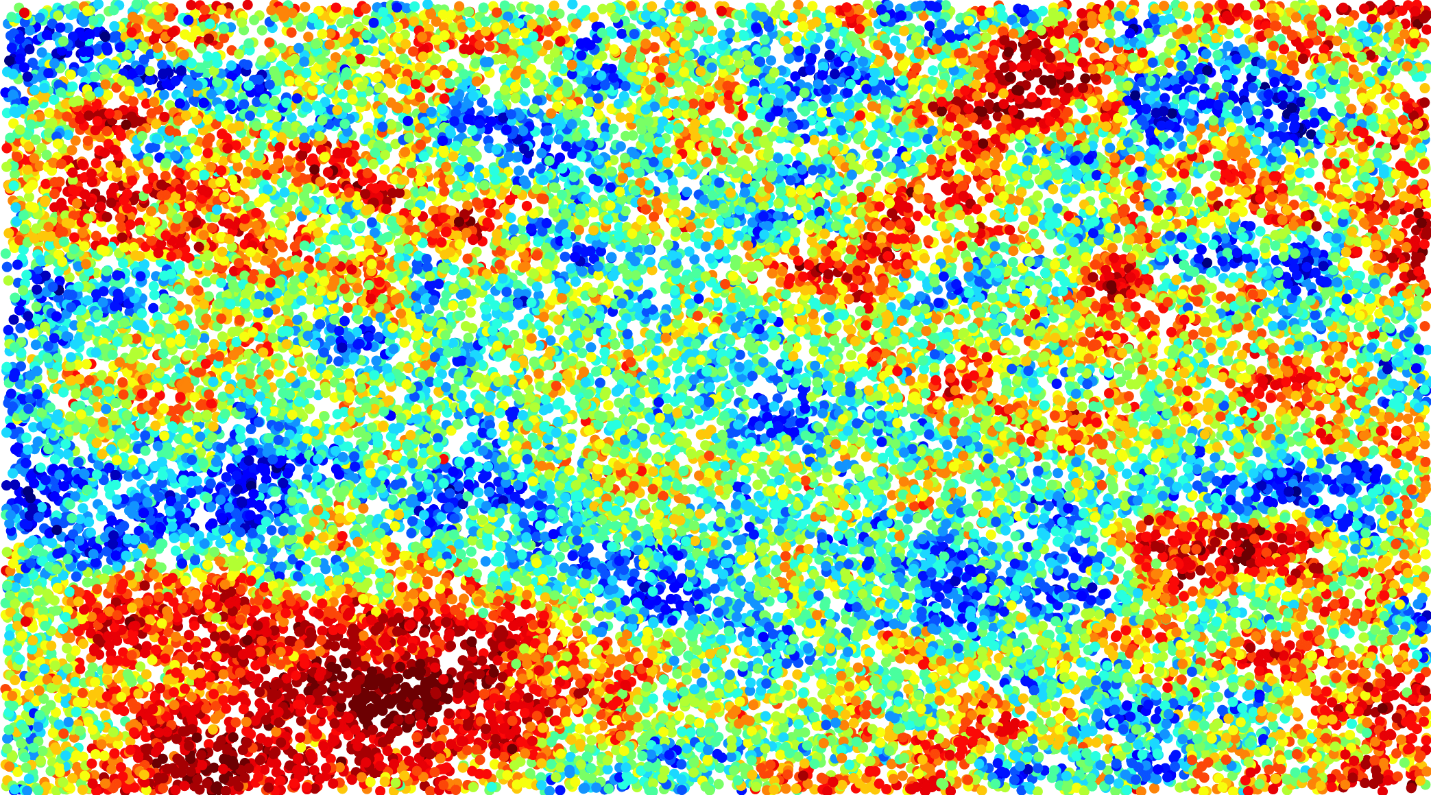
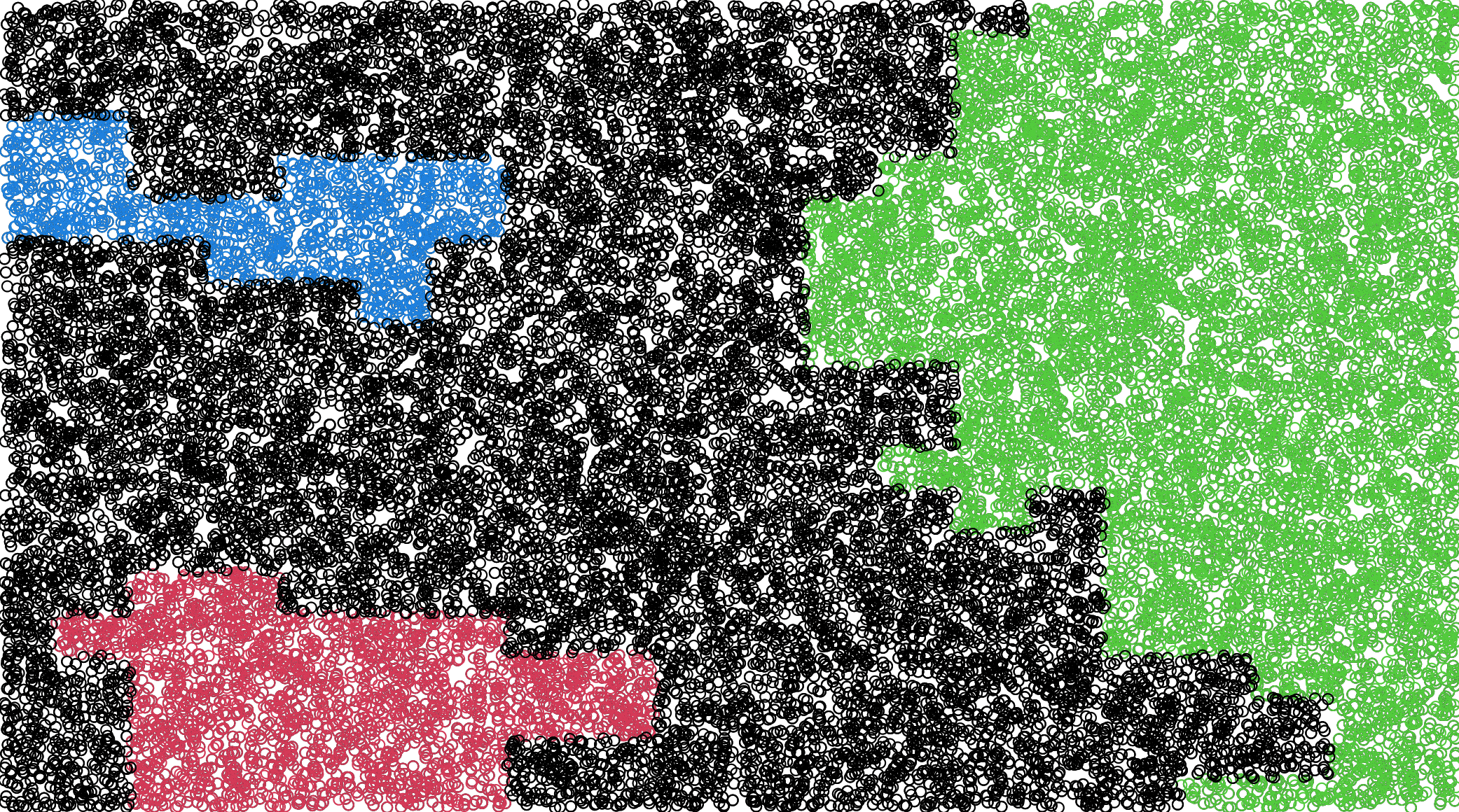
(a) Spatial Surface	(b) Partition of Spatial Domain ($K=4)$
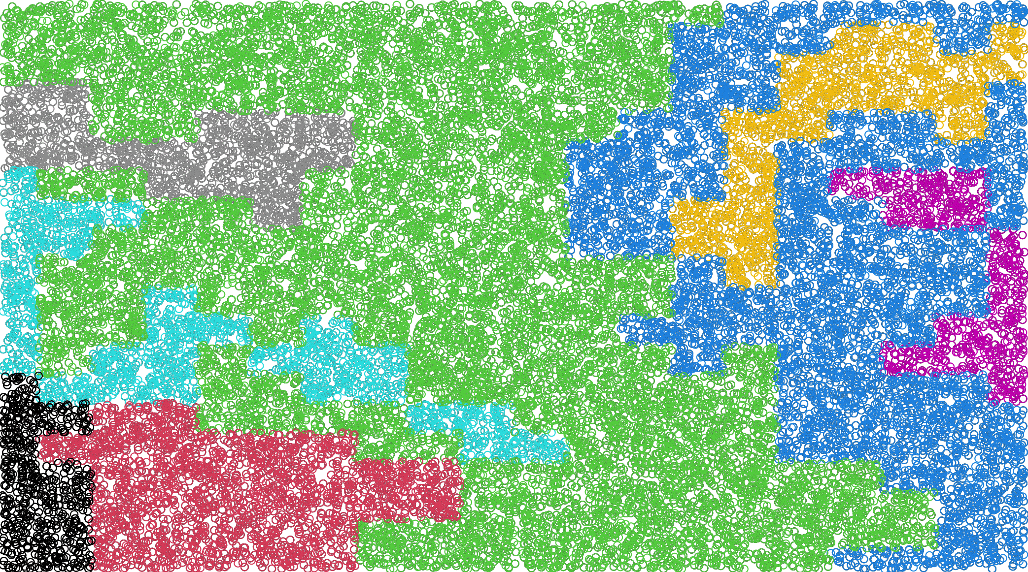
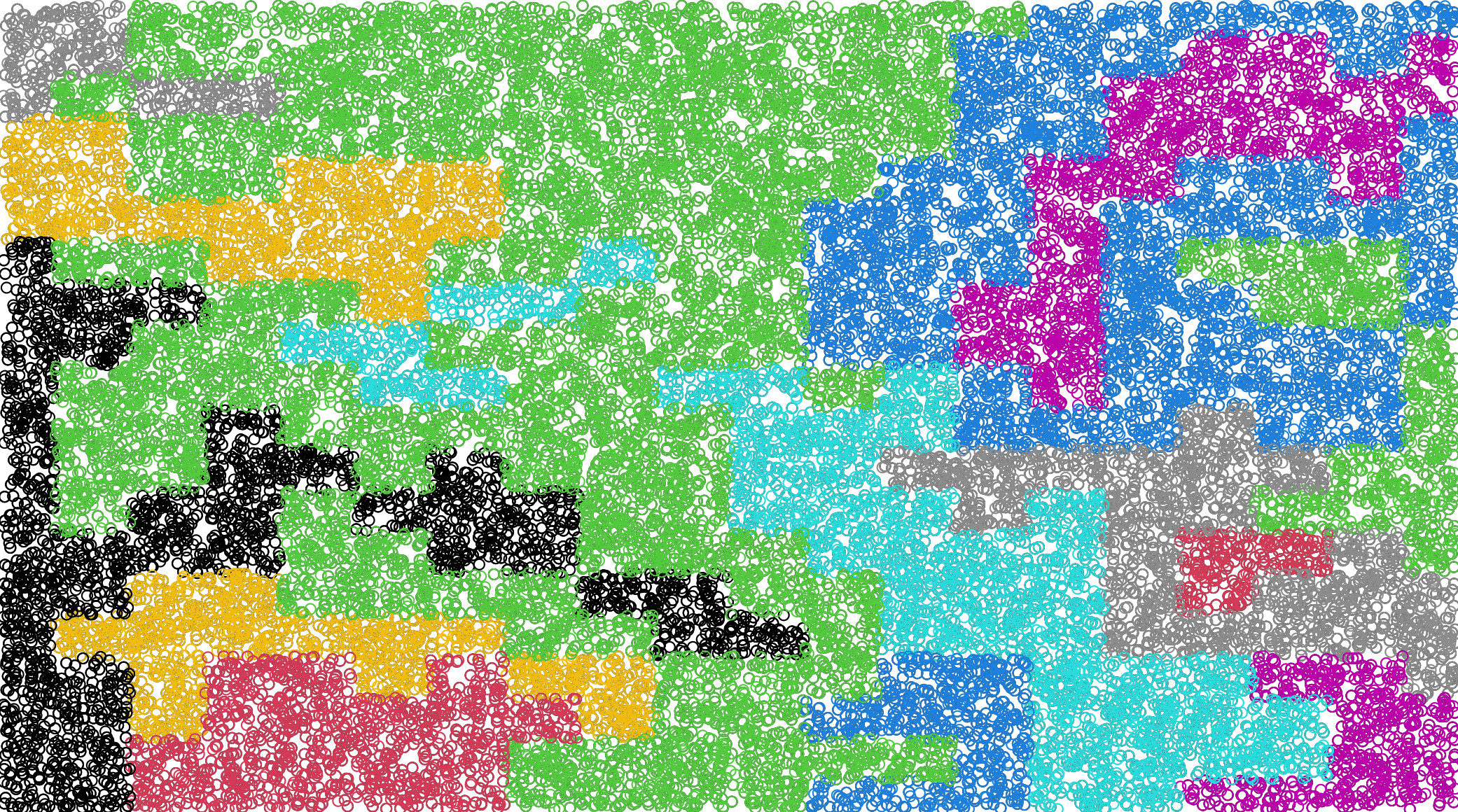
(c) Partition of Spatial Domain ($K=8)$	(d) Partition of Spatial Domain ($K=16)$

Figure 1: Illustration of spatial partitioning. (a) Spatial observations. (b) Observations partitioned into 4 subregions; different colors indicate disjoint partitions. (c) Case for 8 partitions. (d) Case for 16 partitions.

3.2 Bayesian Hierarchical Model

For partition $k=1,\ldots,K$, the conditional mean $\mathbb{E}\left[\bm{Z}_{k}\mid\bm{\beta}_{k},\bm{\delta}_{k},\epsilon_{k},\mathcal{K}_{k},\bm{\gamma}\right]$ is modeled as,

$$\begin{gathered}g\left(\mathbb{E}\left[\bm{Z}_{k}\mid\bm{\beta}_{k},\bm{\delta}_{k},\epsilon_{k},\mathcal{K}_{k},\bm{\gamma}\right]\right):=\bm{\eta}_{k}=\bm{X}_{k}\bm{\beta}_{k}+\bm{\Phi}_{k}(\epsilon_{k},\mathcal{K}_{k})\bm{\delta}_{k}+\bm{H}_{k}\bm{\gamma},\end{gathered}$$ (4)

where $\bm{X}_{k}$ is an $N_{k}\times P$ covariate matrix with corresponding regression coefficients $\bm{\beta}_{k}=(\beta_{k1},\ldots,\beta_{kP})^{\top}$, $\mathcal{K}_{k}=(\bm{u}_{k,1},\ldots,\bm{u}_{k,r_{k}})$ is a vector of partition-specific knots, $\epsilon_{k}$ is a partition-specific bandwidth parameter, $\bm{\Phi}_{k}(\epsilon_{k},\mathcal{K}_{k})$ is an $N_{k}\times r_{k}$ adaptive radial basis function matrix with basis coefficients $\bm{\delta}_{k}=(\delta_{k1},\ldots,\delta_{kr_{k}})^{\top}$, and $\bm{H}_{k}$ is a basis function matrix with global coefficients $\bm{\gamma}=(\gamma_{1},\ldots,\gamma_{G})^{\top}$.

For the combined vector of observations $\bm{Z}=(\bm{Z}_{1}^{\top},\ldots,\bm{Z}_{K}^{\top})^{\top}$, (4) implies that,

$$g\left(\mathbb{E}\left[\bm{Z}\mid\bm{\beta},\bm{\delta},\bm{\epsilon},\mathcal{K},\bm{\gamma}\right]\right):=\bm{\eta}=\bm{X}\bm{\beta}+\bm{\Phi}(\bm{\epsilon},\mathcal{K})\bm{\delta}+\bm{H}\bm{\gamma},$$

where $\bm{X}$ is a block-diagonal matrix with matrices $\bm{X}_{k}$ on the main diagonal, $\bm{\beta}=(\bm{\beta}_{1}^{\top},\ldots,\bm{\beta}_{K}^{\top})^{\top}$, $\bm{\epsilon}=(\epsilon_{1},\ldots,\epsilon_{K})$, $\bm{\Phi}(\bm{\epsilon},\mathcal{K})$ is a block-diagonal matrix with matrices $\bm{\Phi}_{k}(\epsilon_{k},\mathcal{K}_{k})$ on the main diagonal, $\bm{\delta}=(\bm{\delta}_{1}^{\top},\ldots,\bm{\delta}_{K}^{\top})^{\top}$, and $\bm{H}$ is an $N\times G$ matrix stacking the individual $\bm{H}_{k}$ matrices. The parameter $\epsilon_{k}$ determines the smoothness of the basis functions associated with the $k\text{-th}$ partition. By allowing $\epsilon_{k}$ to vary across partitions, our approach can capture the smooth and rough surfaces of the heterogeneous spatial domain.

Since the basis functions (3) are infinitely differentiable, it is possible that the surfaces resulting from the basis expansions will be infinitely smooth. However, we find that letting $\epsilon_{k}$ be sufficiently large obviates this challenge in practical applications. In many applications, it may be desirable to have global regression coefficients such that $\bm{\beta}=\bm{\beta}_{1}=\cdots=\bm{\beta}_{K}$. In that setting, $\bm{X}$ would be an $N\times P$ matrix stacking the $\bm{X}_{k}$ matrices. Using Adapt-BaSeS, the hierarchical spatial model is:

Data Model: $$Z(\bm{s}_{i})\mid\eta(\bm{s}_{i})\sim F(\eta(\bm{s}_{i}))$$ (5)

$$g(\mathbb{E}[\bm{Z}\mid\bm{\beta},\bm{\delta},\bm{\epsilon},\mathcal{K},\bm{\gamma}]):=\bm{\eta}=\bm{X}\bm{\beta}+\bm{\Phi}(\bm{\epsilon},\mathcal{K})\bm{\delta}+\bm{H}\bm{\gamma}$$

Process Model: $$\bm{\delta}_{k}\mid\tau_{k}^{2}\sim\mathcal{N}(\bm{0},\tau_{k}^{2}\mathcal{I})$$

$$\bm{\gamma}\mid\rho^{2}\sim\mathcal{N}(\bm{0},\rho^{2}\mathcal{I})$$

Parameter Model: $$\bm{\beta}_{k}\sim p(\bm{\beta}_{k}),\epsilon_{k}\sim p(\epsilon_{k}),\tau_{k}^{2}\sim p(\tau_{k}^{2}),$$

$$\mathcal{K}_{k}\sim p(\mathcal{K}_{k}),\rho^{2}\sim p(\rho^{2}),$$

where $\mathcal{I}$ denotes the identity matrix. We complete the hierarchical spatial model by specifying the prior distributions for the model parameters $\bm{\beta}_{k}$, $\epsilon_{k}$, $\tau_{k}^{2}$, $\rho^{2}$, and $\mathcal{K}_{k}$. We can reduce computational costs by limiting the number of basis functions $r_{k}$ within each partition to be small and by specifying the covariance matrices $\bm{\Sigma}_{\bm{\delta}_{k}}$ and $\bm{\Sigma}_{\bm{\gamma}}$ to be diagonal (Lee and Park, 2023; Higdon, 1998; Lindgren, Rue and Lindström, 2011; Nychka et al., 2015). It can also be possible to introduce a covariance structure for the basis coefficients, such as an exponential covariance function (Heaton et al., 2019). However, this would result in additional computational overhead. Conditional on $\bm{\gamma}$, the parameters $\bm{\beta}_{k}$, $\mathcal{K}_{k}$, $\bm{\delta}_{k}$, $\epsilon_{k}$, and $\tau_{k}^{2}$ can be estimated independently for each partition. Hence, the MCMC updates of these parameters can be done in parallel to facilitate computational efficiency.

3.3 The Reversible-Jump MCMC Algorithm

We propose a RJMCMC algorithm (Algorithm 1) to select the number and placement of knots within each partition. For a given partition $k$, we take the number of knots $r_{k}$ to be random, from some countable set $\mathcal{S}_{k}=\{0,\ldots,R_{k}\}$, where $R_{k}$ is the number of candidate knots in partition $k$. Let $\mathcal{M}_{r_{k}}$ denote the model with exactly $r_{k}$ knots and let $\mathcal{K}_{k}(r_{k})=\{\bm{u}_{k,1},\ldots,\bm{u}_{k,r_{k}}\}$ denote the knots. We generate samples from the joint posterior of $(r_{k},\mathcal{K}_{k}(r_{k}))$. To account for the varying dimensionality, we must develop appropriate reversible jump moves. For this problem, possible transitions are: (1) add a knot (birth step), (2) delete a knot (death step), and (3) move a knot. These independent move types are randomly chosen with probability $b_{r_{k}}$ for the move $r_{k}$ to $r_{k}+1$ (birth step), $d_{r_{k}}$ for the move $r_{k}$ to $r_{k}-1$ (death step), and $\eta_{r_{k}}$ for the move step. These probabilities must satisfy $b_{r_{k}}+d_{r_{k}}+\eta_{r_{k}}=1$. For this choice, we define $b_{0}=d_{R_{k}}=1$ and $b_{r_{k}}=d_{r_{k}}=\eta_{r_{k}}=1/3$ otherwise.

3.3.1 Prior Specifications

We specify a truncated Poisson prior distribution for $r_{k}$, such that

$$p(r_{k})\propto\frac{\lambda^{r_{k}}\exp(-\lambda)}{r_{k}!}\mathds{1}_{\{0,\ldots,R_{k}\}}(r_{k}).$$

The choice of $\lambda$ is a compromise between model flexibility and model parsimony. A small value of $\lambda$ reflects a strong incidence of smoothness whereas a large value may cause the model to fit the data too closely. The choice of $\lambda$ will be discussed later.

For a given $r_{k}$, the knots are taken to be randomly uniformly selected with state space the candidate knots $\mathcal{R}_{k}=\{\bm{u}_{k,1},\ldots,\bm{u}_{k,R_{k}}\}$, where $\bm{u}_{k,1},\ldots,\bm{u}_{k,R_{k}}$ are distributed equidistantly over subregion $\mathcal{D}_{k}$. Given $r_{k}$, the prior distribution for $\mathcal{K}_{k}(r_{k})=\{\bm{u}_{k,1},\ldots,\bm{u}_{k,r_{k}}\}$ is then given by

$$p(\mathcal{K}_{k}(r_{k})\mid r_{k})={\binom{R_{k}}{r_{k}}}^{-1}=\frac{r_{k}!(R_{k}-r_{k})!}{R_{k}!}.$$

A commonly used prior for regression coefficients of a generalized linear model is the multivariate normal distribution $\bm{\delta}_{k}\mid r_{k}\sim\mathcal{N}(\mathbf{0},\bm{\Sigma}_{\bm{\delta}_{k}})$ (Gamerman, 1997). Following Biller (2000), we assume the basis coefficients $\bm{\delta}_{k}$ are uncorrelated, i.e., $\bm{\Sigma}_{\bm{\delta}_{k}}=\tau_{k}^{2}\mathcal{I}$.

3.3.2 Algorithm

At each step of the RJMCMC algorithm, we propose one of three modifications to the current set of $r_{k}$ knots for each partition $k$:

1. Add a knot (birth step): Draw a new knot $\bm{u}_{k,r_{k}+1}$ uniformly with probability $1/(R_{k}-r_{k})$ from the set of the $R_{k}-r_{k}$ vacant knots. Let $\mathcal{K}_{k}^{*}=\mathcal{K}_{k}\cup\{\bm{u}_{k,r_{k}+1}\}$ be the proposed set of knots, which now has size $r_{k}^{*}=r_{k}+1$.

2. Delete a knot (death step): Select a knot $\bm{u}_{k,J}$ uniformly at random from one of the $r_{k}$ current knots, so it is drawn with probability $1/r_{k}$. Then set $\mathcal{K}_{k}^{*}=\mathcal{K}_{k}\backslash\{\bm{u}_{k,J}\}$ and $r_{k}^{*}=r_{k}-1$.

3. Move a knot (move step): Select a knot $\bm{u}_{k,J}$ uniformly at random to be deleted, and then select a new location $\bm{u}_{k,r_{k}+1}$ from the vacant knots (i.e., where to move the old knot). This results in $\mathcal{K}_{k}^{*}=\{\bm{u}_{k,r_{k}+1}\}\cup\mathcal{K}_{k}\backslash\{\bm{u}_{k,J}\}$ and $r_{k}^{*}=r_{k}$.

Note that when we propose to add a knot $\bm{u}_{k,r_{k}+1}$, a corresponding basis coefficient $\delta_{k,r_{k}+1}^{*}$ will also need to be proposed. Similarly, if we propose to delete a knot $\bm{u}_{k,J}$, the current basis coefficient $\delta_{k,J}$ will be set to $0$. If we propose to move a knot, we will propose changing the current basis coefficient from $\delta_{k,J}$ to $\delta_{k,r_{k}+1}^{*}$. Complete details of the RJMCMC algorithm can be seen in Algorithm 1. Proposition 1 asserts that a sufficient choice for the acceptance probability is given by (6); hence fulfilling the detailed balance condition.

Proposition 1.

The detailed balance condition is satisfied by setting the acceptance probability to be $\min\{1,\alpha\}$, where

$$\alpha=\frac{L(\bm{Z}_{k}\mid\mathcal{K}_{k}^{*},\bm{\delta}_{k}^{*})}{L(\bm{Z}_{k}\mid\mathcal{K}_{k},\bm{\delta}_{k})}\frac{\pi(\mathcal{K}_{k}^{*},\bm{\delta}_{k}^{*})}{\pi(\mathcal{K}_{k},\bm{\delta}_{k})}\frac{Q(\mathcal{K}_{k}^{*},\mathcal{K}_{k})}{Q(\mathcal{K}_{k},\mathcal{K}_{k}^{*})},$$ (6)

and the proposal ratio is given by,

$$\frac{\mathcal{Q}(\mathcal{K}_{k}^{*},\mathcal{K}_{k})}{\mathcal{Q}(\mathcal{K}_{k},\mathcal{K}_{k}^{*})}=\begin{cases}\frac{R_{k}-r_{k}}{r_{k}+1}\times\frac{1}{\mathcal{N}(\delta_{k,r_{k}+1}^{*};0,\sigma^{2})},&r_{k}^{*}=r_{k}+1\\ \frac{r_{k}}{R_{k}-r_{k}+1}\times\mathcal{N}(\delta_{k,J};0,\sigma^{2}),&r_{k}^{*}=r_{k}-1\\ \frac{\mathcal{N}(\delta_{k,J};0,\sigma^{2})}{\mathcal{N}(\delta_{k,r_{k}+1}^{*};0,\sigma^{2})},&r_{k}^{*}=r_{k},\end{cases}$$

and the prior ratio is given by,

$$\frac{\pi(\mathcal{K}_{k}^{*},\bm{\delta}_{k}^{*})}{\pi(\mathcal{K}_{k},\bm{\delta}_{k})}=\begin{cases}\frac{p(r_{k}+1)}{p(r_{k})}\frac{r_{k}+1}{R_{k}-r_{k}}\frac{\mathcal{N}(\delta_{k,r_{k}+1}^{*};0,\tau_{k}^{2})}{\mathcal{N}(0;0,\tau_{k}^{2})},&r_{k}^{*}=r_{k}+1\\ \frac{p(r_{k}-1)}{p(r_{k})}\frac{R_{k}-r_{k}+1}{r_{k}}\frac{\mathcal{N}(0;0,\tau_{k}^{2})}{\mathcal{N}(\delta_{k,J};0,\tau_{k}^{2})},&r_{k}^{*}=r_{k}-1\\ \frac{\mathcal{N}(\delta_{k,r_{k}+1}^{*};0,\tau_{k}^{2})}{\mathcal{N}(\delta_{k,J};0,\tau_{k}^{2})},&r_{k}^{*}=r_{k},\end{cases}$$

where $\sigma^{2}$ is the proposal variance for the basis coefficients. For the special cases where $r_{k}=0$ or $r_{k}=R_{k}$, the respective proposal ratios can be shown to be $R_{k}/(3\mathcal{N}(\delta_{k,r_{k}+1}^{*};0,\sigma^{2}))$ and $(R_{k}\mathcal{N}(\delta_{k,J};0,\sigma^{2}))/3$.
Proof: See Supplement S5.

Algorithm 1 RJMCMC Algorithm

1:for $i\leftarrow 1$ to $B$ do

2:     Metropolis-Hastings updates for $\bm{\beta}_{k}$, $\epsilon_{k}$, and $\bm{\gamma}$

3:     Gibbs updates for $\tau_{k}^{2}$ and $\rho^{2}$

4:     for Partition $k\leftarrow 1$ to $K$ do

5:         Propose to: (1) add; (2) remove; or (3) move a knot with equal probability $p$

6:         Denote proposed vector of knots and coefficients as $\mathcal{K}_{k}^{*}$ and $\bm{\delta}_{k}^{*}$, respectively

7:         Generate $U\sim\text{Unif}(0,1)$

8:         Accept $\mathcal{K}_{k}^{*}$ and $\bm{\delta}_{k}^{*}$ if $U<\min\{1,\alpha\}$ where $\alpha$ is defined in (6).

9:     end for

10:end for

3.4 Prediction

Let $N_{O}$ denote the number of observations used for model-fitting and let $N_{P}$ denote the number of observations used for validation. Upon fitting the hierarchical spatial model on the vector of observed locations $\mathcal{S}_{O}=(\bm{s}_{1},\ldots,\bm{s}_{N_{O}})$, a natural extension is to infer the linear predictor $\eta(\cdot)$ at a vector of prediction locations $\mathcal{S}_{P}=(\bm{s}_{1},\ldots,\bm{s}_{N_{P}})$. Letting $\bm{s}^{*}\in\mathcal{S}_{P}$ be an arbitrary unobserved location residing in partition $k$, we write:

$$\eta(\bm{s}^{*})=\bm{X}_{k}(\bm{s}^{*})^{\top}\bm{\beta}_{k}+\bm{\Phi}_{k}(\bm{s}^{*};\epsilon_{k},\mathcal{K}_{k})^{\top}\bm{\delta}_{k}+\bm{H}_{k}(\bm{s}^{*})^{\top}\bm{\gamma},$$

where $\bm{X}_{k}(\bm{s}^{*})$ is the covariate vector evaluated at location $\bm{s}^{*}$, $\bm{\Phi}_{k}(\bm{s}^{*};\epsilon_{k},\mathcal{K}_{k})$ is the adaptive basis function vector with corresponding basis coefficients $\bm{\delta}_{k}$, and $\bm{H}_{k}(\bm{s}^{*})$ is the global basis function vector with corresponding global basis coefficients $\bm{\gamma}$. We approximate the posterior predictive distribution for $\eta(\bm{s}^{*})$ using posterior samples $\{\bm{\beta}_{k},\epsilon_{k},\bm{\delta}_{k},\mathcal{K}_{k},\bm{\gamma}\}$. As with the parameter estimation, we note that the predictions are made within each cluster and hence can be done in parallel to promote computational efficiency. Furthermore, the posterior distribution allows for uncertainty quantification by evaluating the variance of the posterior samples.

3.5 Implementation Details

Our method requires tuning three parameters: (1) the number of partitions $K$; (2) the prior rate parameter $\lambda$ for the number of basis functions to be used within each partition; and (3) the prior distribution for the partition-specific bandwidths $\bm{\epsilon}=\{\epsilon_{k}\}_{k=1}^{K}$. Selecting a small value of $K$ may not be adequate for approximating nonstationary spatial processes because there may be several heterogeneous subregions within the spatial domain. On the other hand, selecting a large value of $K$ may result in many partitions with a small number of observations $N_{k}$. In our simulation study, we compare the performance of our method with various choices of $K$. For the partition-specific bandwidths, we specify a uniform prior $\epsilon_{k}\sim\text{Unif}(\alpha,\beta)$ to allow for control over the range of possible values $\epsilon_{k}$ can take on. For $\mathcal{D}=[0,5]^{2}$, a sensitivity analysis suggests that $\alpha=0.01$ and $\beta=3$ provides a suitable range of values for $\epsilon_{k}$ to accommodate both smooth and rough partitions. A truncated Poisson distribution with prior rate parameter $\lambda$ is used for the number of basis functions for each partition. A sensitivity analysis suggests that results are relatively insensitive to choices of $\lambda$ in the range 5-20 so we choose $\lambda=5$ to promote parsimony and computational efficiency. We set the priors for $\bm{\beta}$ and $\tau_{k}^{2}$ following (Hughes and Haran, 2013): $\bm{\beta}\sim\mathcal{N}(\bm{0},100\mathcal{I})$ and $\tau_{k}^{2}\sim\mathsf{IG}(0.5,2000)$. The latter prior is desirable because it corresponds to the prior belief that the fixed effects are sufficient for explaining the data. For the global basis function matrix $\bm{H}$, we use three layers of nested bisquare basis functions (Sengupta et al., 2016).

4 Simulation Study

In this section, we demonstrate the Adapt-BaSeS approach through an extensive simulation study featuring multiple spatial data classes and dependence structures. To benchmark performance, we compare our approach with two competing methods.

4.1 Simulation Study Design

Let $\bm{s}_{i}\in\mathcal{D}=[0,5]^{2}\subset\mathbb{R}^{2}$ for $i=1,\ldots,N$ denote the spatial locations and let $\mathcal{\bm{S}}=(\bm{s}_{1},\ldots,\bm{s}_{N})$. On these locations, let $\bm{Z}=(Z(\bm{s}_{1}),\ldots,Z(\bm{s}_{N}))^{\top}$ denote the vector of response variables (i.e., the data). For model fitting, we use $N_{O}=5{,}000$ observations and reserve $N_{P}=1{,}000$ observations for validation. We consider both binary and count data, with the associated spatial random effects generated from both nonstationary and stationary spatial processes. Observations are generated using the SGLMM framework described in (1) with $X_{1},X_{2}\sim\text{Unif}(-0.5,0.5)$ and $\bm{\beta}=(1,1)$. We study our method for $K=\{9,16,25,36,49\}$ partitions. All together, we study a total of $5\times 2\times 2=20$ implementations.

The nonstationary spatial random effects $\bm{W}=\{W(\bm{s}_{i}):\bm{s}_{i}\in\mathcal{D}\}$ are generated by smoothing several locally stationary processes (Fuentes, 2001). Further details are provided in the supplementary material. The stationary spatial random effects are generated using an exponential covariance function with scaling parameter $\phi=1$ and partial sill parameter $\sigma^{2}=1$. The binary datasets use a Bernoulli data model and a logit link function and the count datasets are generated using a Poisson data model and a log link function. For each data generation mechanism (4 total), we generate 100 replicate data sets.

We fit the model using the hierarchical framework outlined in (5). We generate $100{,}000$ samples from the posterior distribution $\pi(\bm{\beta},\epsilon_{k},\mathcal{K}_{k},\bm{\delta}_{k},\tau_{k}^{2},\rho^{2})$ for $k=1,\ldots,K$ using the RJMCMC algorithm described in Algorithm 1. To evaluate predictive performance, we compute the average root cross-validated mean squared prediction error (rCVMSPE), defined as $\text{rCVMSPE}=\left(\frac{1}{N_{P}}\sum_{i=1}^{N_{P}}\left(Z_{i}-\hat{Z}_{i}\right)^{2}\right)^{1/2}$, the area under the receiver operating curve (AUC) for the binary case, and the walltime (computation time) required to run $100{,}000$ iterations of the RJMCMC algorithm.

Fitting a “gold standard” SGLMM (1) is prohibitive due to the overparameterized model and large matrix operations. Hence, we compare our approach with two competing methods: the NNGP approach and a fixed bisquare basis function approach. The computation times are based on a single 2.4 GHz Intel Xeon Gold 6240R processor provided by GMU’s HOPPER high-performance computing infrastructure.

4.2 Simulation Study Results

Table 1 and Table 2, respectively, present the rCVMSPE and AUC for Adapt-BaSeS and the competing approaches. The results indicate that our method yields more accurate predictions than the competing methods across different values of $K$, data classes, and covariance structures. Paired $t$-tests were performed to compare the sets of rCVMSPE’s between our approach and the competing methods. The corresponding $p$-values were found to be statistically significant, with $p<0.001$ for each pairwise comparison. Predictive performance generally improves as we increase the number of partitions $K$. However, the predictive standard deviations generally increase with larger $K$. For one simulated nonstationary dataset, we present the posterior predictive log intensity surface (Figure 2) and the posterior predictive probability surface (Figure 3) obtained from the implementation yielding the lowest rCVMSPE ($K=49$). Based on a visual inspection, our method successfully captures the nonstationary behavior of the true latent spatial process in both cases. Plots illustrating the prediction standard deviations can be found in the supplementary material.

The model-fitting walltimes are reported in the supplementary material. The proposed approach exhibits higher computational costs than the fixed basis function approach. However, our method is more computationally efficient than the NNGP approach. The shorter walltimes for the fixed basis function approach are expected since the spatial basis functions are fixed prior to model-fitting. In contrast, our proposed method modifies the spatial basis functions at each iteration of the RJMCMC algorithm, leading to increased computational costs. Despite the longer walltimes, our approach offers additional flexibility in modeling the latent spatial process and yields more accurate predictions. Importantly, both approaches provide substantial improvements in computational efficiency over the “gold standard” SGLMM (1), which would be computationally infeasible for a dataset with $N_{O}=5{,}000$ observations.

	Nonstationary			Stationary
Method	Poisson	Binary		Poisson	Binary
Bisquare	1.817 (0.140)	0.478 (0.045)		1.754 (0.143)	0.460 (0.044)
NNGP		0.474 (0.131)			0.458 (0.123)
$K=9$	1.719 (0.156)	0.470 (0.042)		1.709 (0.128)	0.453 (0.043)
$K=16$	1.700 (0.174)	0.468 (0.043)		1.650 (0.180)	0.451 (0.042)
$K=25$	1.688 (0.192)	0.466 (0.045)		1.648 (0.195)	0.450 (0.044)
$K=36$	1.682 (0.206)	0.465 (0.048)		1.639 (0.213)	0.449 (0.047)
$K=49$	1.680 (0.224)	0.464 (0.052)		1.633 (0.232)	0.448 (0.051)

Table 1: Average rCVMSPE for the simulation study. Columns correspond to the data class and spatial dependence structure. Results are presented for various choices of $K$. Top rows correspond the fixed basis functions approach and NNGP. Average standard deviation of the predictions are provided in parentheses.

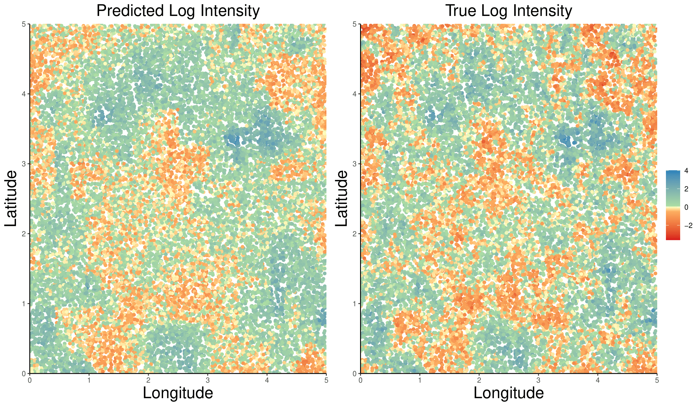
Figure 2: Predicted (left) and true (right) log intensity surface for one nonstationary validation sample for the count data case.

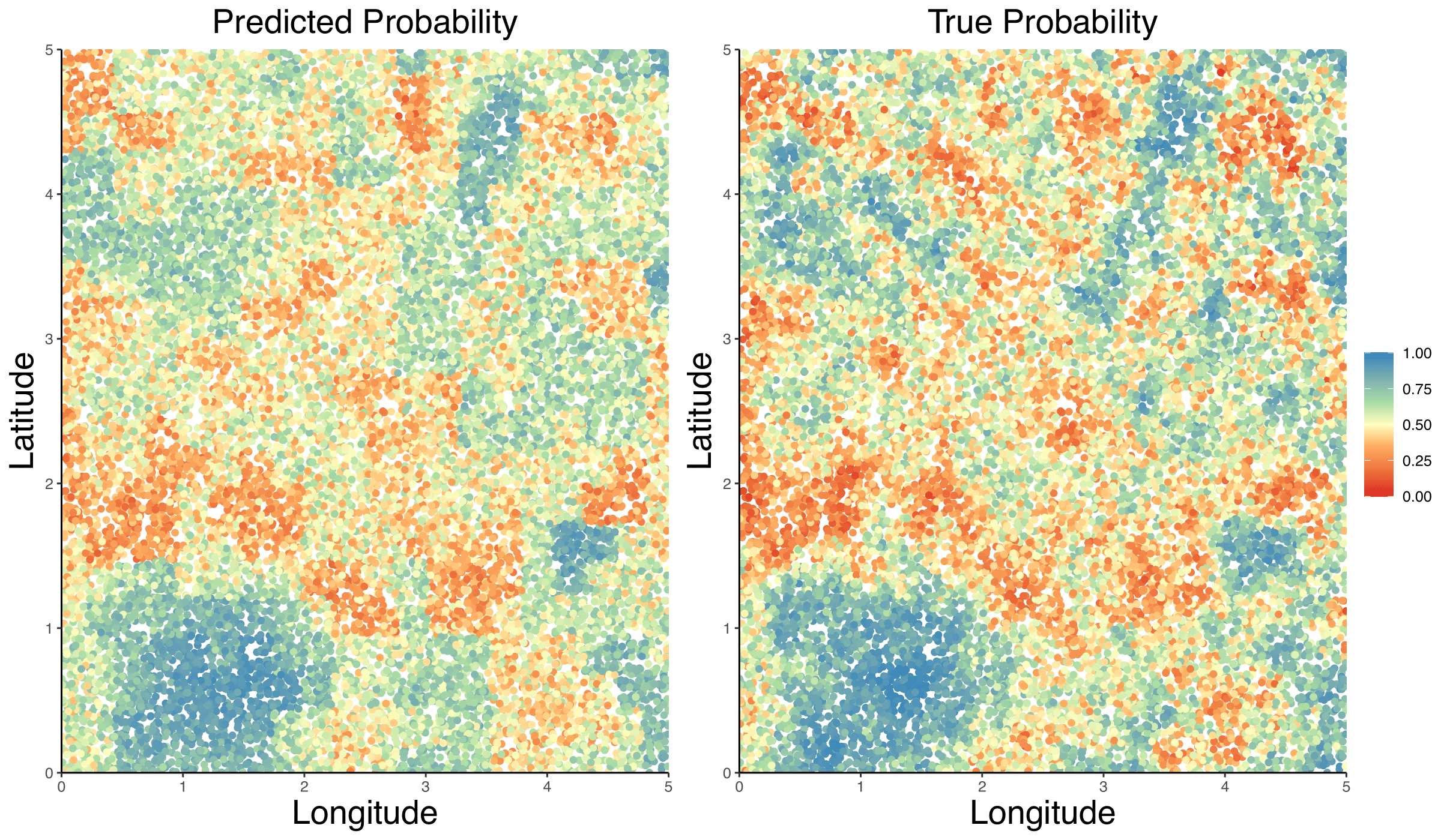
Figure 3: Predicted (left) and true (right) probability surface for one nonstationary validation sample for the binary data case.

Method	Nonstationary	Stationary
Bisquare	0.663	0.711
NNGP	0.679	0.716
$K=9$	0.693	0.731
$K=16$	0.700	0.736
$K=25$	0.706	0.740
$K=36$	0.709	0.742
$K=49$	0.711	0.743

Table 2: Out-of-sample area under the receiver operating curve (AUC)

5 Applications

In this section, we apply the Adapt-BaSeS to two real-world spatial datasets: binary incidence of dwarf mistletoe in Minnesota (Hanks, Hooten and Baker, 2011) and counts from the North American Breeding Bird Survey (BBS) (Ziolkowski et al., 2022).

5.1 Binary Data: Parasitic Infestation of Dwarf Mistletoe

The dwarf mistletoe is a parasitic species that extracts key resources from its host, such as the black spruce species (Geils and Hawksworth, 2002). This infestation poses economic challenges, because black spruce is a valuable resource for producing high-quality paper. We apply our method to analyze dwarf mistletoe incidence data in Minnesota, obtained from the Minnesota Department of Natural Resources operational inventory (Hanks, Hooten and Baker, 2011). The dataset contains binary incidence of dwarf mistletoe at $N=25{,}431$ locations, with dwarf mistletoe being present at $2{,}872$ of these locations. We fit the model on $N_{O}=12{,}931$ observations and set aside $N_{P}=12{,}500$ observations for validation. We consider several covariates as inputs to our model, including: (1) the average age of trees in years; (2) basal area per acre of trees in the stand; (3) average canopy height; and (4) volume of the stand measured in cords. We study the performance of our method for $K\in\{9,16,25,36\}$.

For each implementation, we compute the rCVMSPE and the AUC for the binary classification (Table 3). We observe that increasing the number of partitions improves the predictive performance of our proposed approach. Specifically, using $K=36$ partitions yields the highest AUC value and the lowest rCVMSPE. In contrast, the fixed basis function approach provides less accurate predictions compared to our proposed method, across all four partition levels. Figure 4 displays the predictive probability surface and the true binary observations for the validation sample, for the case of $K=36$.

Method	rCVMSPE	AUC
Bisquare	0.308 (0.015)	0.734
$K=9$	0.300 (0.017)	0.764
$K=16$	0.296 (0.022)	0.785
$K=25$	0.295 (0.023)	0.790
$K=36$	0.294 (0.024)	0.793

Table 3: rCVMSPE and AUC for the dwarf mistletoe dataset. Results are presented for varying number of partitions $K$. The top row corresponds to the fixed basis function approach. The average standard deviation of the predictions are provided in parentheses.

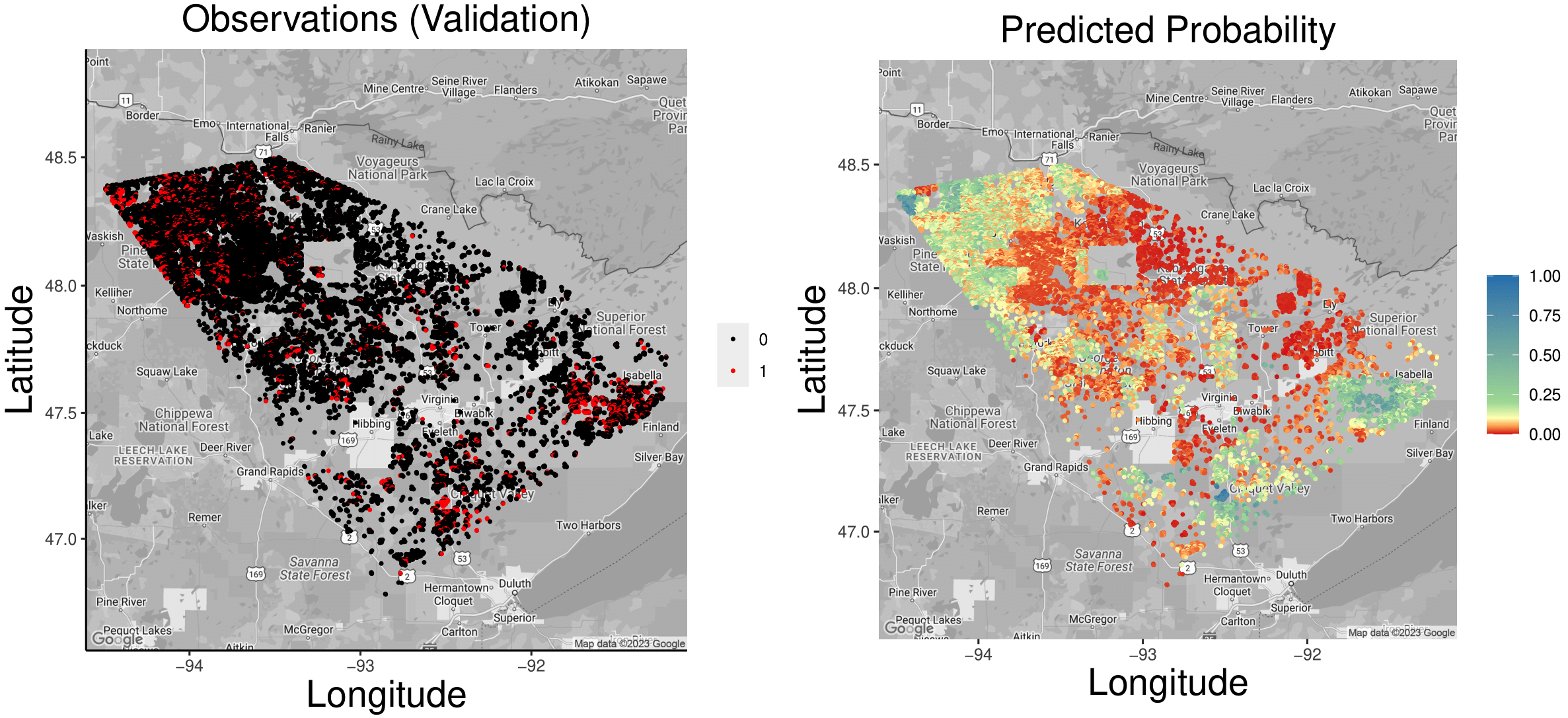
Figure 4: Illustration of the dwarf mistletoe occurrence dataset for $K=36$. True observations (left) and posterior predictive probability surface (right) for the validation sample.

5.2 Count Data: North American Breeding Bird Survey 2018

The Bird Breeding Survey (BBS) (Ziolkowski et al., 2022) is an annual roadside survey that involves trained observers monitoring the abundance of bird populations in North America. The sum of counts serves as an index of species abundance along the route for that specific year. The particular BBS dataset includes Blue Jay (Cyanocitta cristata) bird counts at a total of $N=1{,}593$ locations, covering eastern and central regions of the United States. We use $N_{O}=1{,}000$ observations to fit the model and reserve $N_{P}=593$ for validation. We fit the model with only the spatial random effects (i.e., the conditional mean is modeled as $g(\mathbb{E}[Z(\mathbf{s}_{i})])=W(\cdot)$ and does not include spatial covariates).

Table 4 displays the rCVMSPE for each implementation. We find that our method consistently outperforms the fixed basis function approach. For the case of $K=9$ partitions, Figure 5 displays the true count observations and the predictive intensity surface, obtained from $k$-fold cross-validation. The predictive intensity map reveals that Blue Jays are most abundant in the southeastern and northeastern regions of the United States.

Method	rCVMSPE
Bisquare	8.735 (0.706)
$K=5$	8.599 (0.735)
$K=6$	8.583 (0.857)
$K=7$	8.537 (0.892)
$K=8$	8.515 (1.013)
$K=9$	8.572 (0.904)

Table 4: rCVMSPE for the Blue Jay spatial count dataset. Results are presented for varying $K$. Results from fixed basis functions are in the top row. Average standard deviation of predictions are in parentheses.

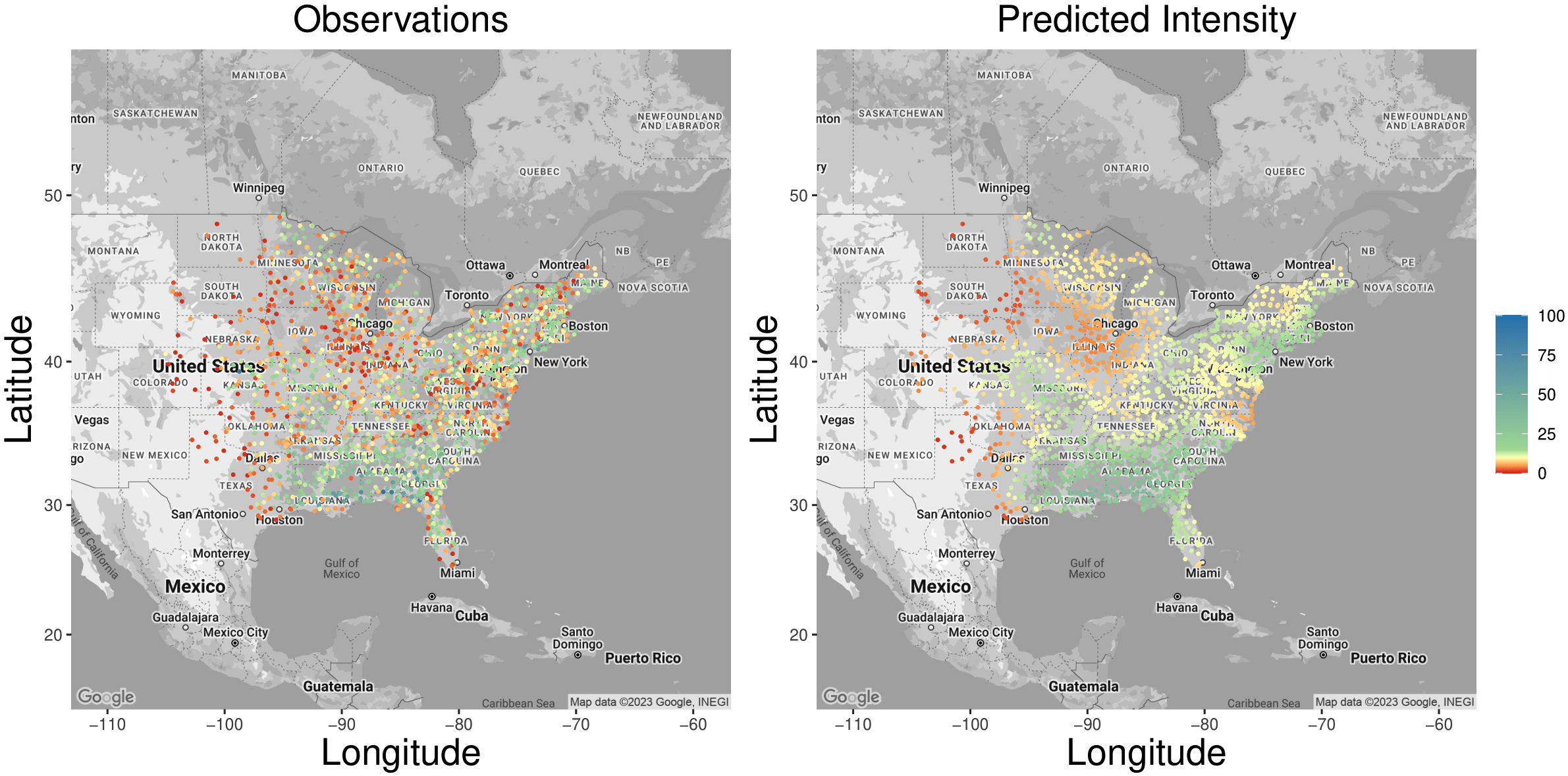
Figure 5: Illustration of the Blue Jay count dataset for $K=9$. True observations (left) and posterior predictive intensity surface (right).

6 Discussion

We propose a data-informed, flexible, and computationally efficient method to model high-dimensional non-Gaussian spatial observations with nonstationary spatial dependence structures. Past studies have used spatial radial basis functions; thereby accounting for nonstationarity and reducing computational costs. However, these studies generally fix crucial components of the basis functions, such as the number of basis functions, placement of basis knots, and bandwidth (smoothing) parameters, perhaps arbitrarily, before fitting the model.

Our fast yet flexible method partitions the spatial domain into disjoint subregions using an agglomerative spatial clustering algorithm (Heaton, Christensen and Terres, 2017). We then employ a RJMCMC algorithm to select critical features (knots and bandwidths) of the basis functions within each partition. Results from both our simulation study and real-world applications demonstrate that our approach performs well in both inference and predictions over competing methods, while also preserving computational efficiency.

While our proposed adaptive framework primarily focuses on Gaussian radial basis functions, it can be extended to accommodate a wider range of radial basis functions. This includes thin-plate-spline basis functions, multiquadric radial basis functions, and bisquare basis functions, among others. Though our approach offers a significant speedup compared to the “gold standard” SGLMM (1), the computational speedup can be further enhanced by embedding sparse basis functions such as the Wendland basis functions (Nychka et al., 2015) or multi-resolution approximation (M-RA) basis functions (Katzfuss, 2017), which can drastically reduce the number of floating point operations. In a similar strain, the embarrassingly parallel matrix operations can be distributed across available processors (Guan and Haran, 2018) in high-performance computing systems.

Supplementary Material

The supplementary material includes: (1) details on the construction of the bisquare basis functions as well as a visualization of the multi-resolution “quad-tree” structure; (2) details on the clustering algorithm (Heaton, Christensen and Terres, 2017); (3) model-fitting walltimes for the simulation study; (4) a proof of the detailed balance proposition; and (5) visualizations of the prediction standard deviation surfaces.

References

- Banerjee, Carlin and Gelfand (2003) Banerjee, S., Carlin, B. P. and Gelfand, A. E. (2003). Hierarchical Modeling and Analysis for Spatial Data. 2nd Edition. Chapman and Hall/CRC, New York.
- Banerjee et al. (2008) Banerjee, S., Gelfand, A. E., Finley, A. O. and Sang, H. (2008). Gaussian predictive process models for large spatial data sets. Journal of the Royal Statistical Society: Series B (Statistical Methodology) 70(4), 825–848.
- Biller (2000) Biller, C. (2000). Adaptive Bayesian regression splines in semiparametric generalized linear models. Journal of Computational and Graphical Statistics 9(1), 122–140.
- Bradley, Cressie and Shi (2011) Bradley, J. R., Cressie, N. and Shi, T. (2011). Selection of rank and basis functions in the spatial random effects model. In Proceedings of the 2011 Joint Statistical Meetings, 3393-3406. Alexandria, VA: American Statistical Association.
- Brooks et al. (2011) Brooks, S., Gelman, A., Jones, G., and Meng, X. L. (2011). Handbook of Markov Chain Monte Carlo. Chapman and Hall/CRC, Boca Raton.
- Chaudhuri et al. (2017) Chaudhuri, A., Kakde, D., Sadek, C., Gonzalez, L. and Kong, S. (2017). The mean and median criteria for kernel bandwidth selection for support vector data description. In 2017 IEEE International Conference on Data Mining Workshops (ICDMW), 842-849. New Orleans, LA: Institute of Electrical and Electronics Engineers.
- Cressie (1993) Cressie, N. (1993). Statistics for Spatial Data: Wiley Series in Probability and Statistics. Revised Edition. John Wiley & Sons, New York.
- Cressie and Johannesson (2006) Cressie, N. and Johannesson, G. (2006). Spatial prediction for massive datasets. In Mastering the Data Explosion in the Earth and Environmental Sciences: Proceedings of the Australian Academy of Science Elizabeth and Frederick White Conference, 1–11. Canberra, Australia: Australian Academy of Science.
- Cressie and Johannesson (2008) Cressie, N. and Johannesson, G. (2008). Fixed rank kriging for very large spatial data sets. Journal of the Royal Statistical Society: Series B (Statistical Methodology) 70(1), 209–226.
- Cressie, Sainsbury-Dale and Zammit-Mangion (2022) Cressie, N., Sainsbury-Dale, M. and Zammit-Mangion, A. (2022). Basis-function models in spatial statistics. Annual Review of Statistics and Its Application 9, 373–400.
- Cressie and Wikle (2011) Cressie, N. and Wikle, C. K. (2011). Statistics for Spatio-Temporal Data. 1st Edition. John Wiley & Sons, Hoboken.
- Damodaran (2018) Damodaran, B. B. (2018). Fast optimal bandwidth selection for RBF kernel using reproducing kernel Hilbert space operators for kernel based classifiers. arXiv preprint arXiv:1804.05214.
- Datta et al. (2016) Datta, A., Banerjee, S., Finley, A. O. and Gelfand, A. E. (2016). Hierarchical nearest-neighbor Gaussian process models for large geostatistical datasets. Journal of the American Statistical Association 111(514), 800–812.
- Diggle, Tawn and Moyeed (1998) Diggle, P. J., Tawn, J. A. and Moyeed, R. A. (1998). Model-based geostatistics. Journal of the Royal Statistical Society: Series C (Applied Statistics) 47(3), 299–350.
- Dovers et al. (2023) Dovers, E., Brooks, W., Popovic, G. C. and Warton, D. I. (2023). Fast, approximate maximum likelihood estimation of log-Gaussian Cox processes. Journal of Computational and Graphical Statistics, 1–11.
- Ejigu et al. (2020) Ejigu, B. A., Wencheko, E., Moraga, P. and Giorgi, E. (2020). Geostatistical methods for modelling non-stationary patterns in disease risk. Spatial Statistics 35, 100397–100415.
- Ferkingstad and Rue (2015) Ferkingstad, E. and Rue, H. (2015). Improving the INLA approach for approximate Bayesian inference for latent Gaussian models. Electronic Journal of Statistics 9(2), 2706-2731.
- Finley et al. (2009) Finley, A. O., Sang, H., Banerjee, S. and Gelfand, A. E. (2009). Improving the performance of predictive process modeling for large datasets. Computational Statistics & Data Analysis 53(8), 2873–2884.
- Fuentes (2001) Fuentes, M. (2001). A high frequency kriging approach for non-stationary environmental processes. Environmetrics 12(5), 469–483.
- Furrer, Genton and Nychka (2006) Furrer, R., Genton, M. G. and Nychka, D. (2006). Covariance tapering for interpolation of large spatial datasets. Journal of Computational and Graphical Statistics 15(3), 502–523.
- Gamerman (1997) Gamerman, D. (1997). Sampling from the posterior distribution in generalized linear mixed models. Statistics and Computing 7, 57–68.
- Geils and Hawksworth (2002) Geils, B. W. and Hawksworth, F. G. (2002). Damage, effects, and importance of dwarf mistletoes. In US Department of Agriculture, Forest Service, Rocky Mountain Research Station, Chapter 5, 57-65. Ogden, UT.
- Green (1995) Green, P. J. (1995). Reversible jump Markov chain Monte Carlo computation and Bayesian model determination. Biometrika 82(4), 711–732.
- Guan and Haran (2018) Guan, Y. and Haran, M. (2018). A computationally efficient projection-based approach for spatial generalized linear mixed models. Journal of Computational and Graphical Statistics 27(4), 701–714.
- Hanks, Hooten and Baker (2011) Hanks, E. M., Hooten, M. B. and Baker, F. A. (2011). Reconciling multiple data sources to improve accuracy of large-scale prediction of forest disease incidence. Ecological Applications 21(4), 1173–1188.
- Haran (2011) Haran, M. (2011). Gaussian random field models for spatial data. In Handbook of Markov Chain Monte Carlo, 449–478. Chapman and Hall/CRC, Boca Raton.
- Haran, Hodges and Carlin (2003) Haran, M., Hodges, J. S. and Carlin, B. P. (2003). Accelerating computation in Markov random field models for spatial data via structured MCMC. Journal of Computational and Graphical Statistics 12(2), 249–264.
- Heaton, Christensen and Terres (2017) Heaton, M. J., Christensen, W. F. and Terres, M. A. (2017). Nonstationary Gaussian process models using spatial hierarchical clustering from finite differences. Technometrics 59(1), 93–101.
- Heaton et al. (2019) Heaton, M. J., Datta, A., Finley, A. O., Furrer, R., Guinness, J., Guhaniyogi, R., Gerber, F., Gramacy, R. B., Hammerling, D., Katzfuss, M., Lindgren, F., Nychka, D. W., Sun, F. and Zammit-Mangion, A. (2019). A case study competition among methods for analyzing large spatial data. Journal of Agricultural, Biological and Environmental Statistics 24, 398–425.
- Higdon (1998) Higdon, D. (1998). A process-convolution approach to modelling temperatures in the North Atlantic Ocean. Environmental and Ecological Statistics 5(2), 173–190.
- Holland et al. (1999) Holland, D. M., Saltzman, N., Cox, L. H. and Nychka, D. (1999). Spatial prediction of sulfur dioxide in the eastern United States. In geoENV II-Geostatistics for Environmental Applications: Proceedings of the Second European Conference on Geostatistics for Environmental Applications, 65–76. Valencia, Spain: Springer Netherlands.
- Hughes and Haran (2013) Hughes, J. and Haran, M. (2013). Dimension reduction and alleviation of confounding for spatial generalized linear mixed models. Journal of the Royal Statistical Society: Series B (Statistical Methodology) 75(1), 139–159.
- Kato and Shiohama (2009) Kato, R. and Shiohama, T. (2009). Model and variable selection procedures for semiparametric time series regression. Journal of Probability and Statistics 2009.
- Katzfuss (2013) Katzfuss, M. (2013). Bayesian nonstationary spatial modeling for very large datasets. Environmetrics 24(3), 189–200.
- Katzfuss (2017) Katzfuss, M. (2017). A multi-resolution approximation for massive spatial datasets. Journal of the American Statistical Association 112(517), 201–214.
- Katzfuss and Cressie (2011) Katzfuss, M. and Cressie, N. (2011). Spatio-temporal smoothing and EM estimation for massive remote-sensing data sets. Journal of Time Series Analysis 32(4), 430–446.
- Katzfuss and Cressie (2012) Katzfuss, M. and Cressie, N. (2012). Bayesian hierarchical spatio-temporal smoothing for very large datasets. Environmetrics 23(1), 94–107.
- Lee and Park (2023) Lee, B. S. and Park, J. (2023). A scalable partitioned approach to model massive nonstationary non-Gaussian spatial datasets. Technometrics 65(1), 105–116.
- Lindgren and Rue (2015) Lindgren, F. and Rue, H. (2015). Bayesian spatial modelling with R-INLA. Journal of Statistical Software 63(19), 1–25.
- Lindgren, Rue and Lindström (2011) Lindgren, F., Rue, H. and Lindström, J. (2011). An explicit link between Gaussian fields and Gaussian Markov random fields: the stochastic partial differential equation approach. Journal of the Royal Statistical Society: Series B (Statistical Methodology) 73(4), 423–498.
- Nychka et al. (2015) Nychka, D., Bandyopadhyay, S., Hammerling, D., Lindgren, F. and Sain, S. (2015). A multiresolution Gaussian process model for the analysis of large spatial datasets. Journal of Computational and Graphical Statistics 24(2), 579–599.
- Risser (2016) Risser, M. D. (2016). Nonstationary spatial modeling, with emphasis on process convolution and covariate-driven approaches. arXiv preprint arXiv:1610.02447.
- Royle and Wikle (2005) Royle, J. A. and Wikle, C. K. (2005). Efficient statistical mapping of avian count data. Environmental and Ecological Statistics 12(2), 225–243.
- Schabenberger and Gotway (2005) Schabenberger, O. and Gotway, C. A. (2005). Statistical Methods for Spatial Data Analysis. 1st Edition. Chapman and Hall/CRC, Boca Raton.
- Sengupta and Cressie (2013) Sengupta, A. and Cressie, N. (2013). Hierarchical statistical modeling of big spatial datasets using the exponential family of distributions. Spatial Statistics 4, 14–44.
- Sengupta et al. (2016) Sengupta, A., Cressie, N., Kahn, B. H. and Frey, R. (2016). Predictive inference for big, spatial, non-Gaussian data: MODIS cloud data and its change-of-support. Australian & New Zealand Journal of Statistics 58(1), 15–45.
- Sheather and Jones (1991) Sheather, S. J. and Jones, M. C. (1991). A reliable data-based bandwidth selection method for kernel density estimation. Journal of the Royal Statistical Society: Series B (Methodological) 53(3), 683–690.
- Vecchia (1988) Vecchia, A. V. (1988). Estimation and model identification for continuous spatial processes. Journal of the Royal Statistical Society: Series B (Methodological) 50(2), 297–312.
- Xu, Wikle and Fox (2005) Xu, K., Wikle, C. K. and Fox, N. I. (2005). A kernel-based spatio-temporal dynamical model for nowcasting weather radar reflectivities. Journal of the American Statistical Association 100(472), 1133–1144.
- Zhang (2002) Zhang, H. (2002). On estimation and prediction for spatial generalized linear mixed models. Biometrics 58(1), 129–136.
- Zilber and Katzfuss (2021) Zilber, D. and Katzfuss, M. (2021). Vecchia–Laplace approximations of generalized Gaussian processes for big non-Gaussian spatial data. Computational Statistics & Data Analysis 153, 107081.
- Ziolkowski et al. (2022) Ziolkowski Jr., D., Lutmerding, M., Aponte, V. I. and Hudson, M.-A. (2022). North American Breeding Bird survey dataset 1966-2021: U.S. Geological Survey data release.
- Williams and Rasmussen (2006) Williams, C. K. and Rasmussen, C. E. (2006). Gaussian Processes for Machine Learning. Volume 2. MIT Press, Cambridge.