Adversarial and Random Transformations for Robust Domain Adaptation and Generalization

Abstract

Data augmentation has been widely used to improve generalization in training deep neural networks. Recent works show that using worst-case transformations or adversarial augmentation strategies can significantly improve the accuracy and robustness. However, due to the non-differentiable properties of image transformations, searching algorithms such as reinforcement learning or evolution strategy have to be applied, which are not computationally practical for large scale problems. In this work, we show that by simply applying consistency training with random data augmentation, state-of-the-art results on domain adaptation (DA) and generalization (DG) can be obtained. To further improve the accuracy and robustness with adversarial examples, we propose a differentiable adversarial data augmentation method based on spatial transformer networks (STN). The combined adversarial and random transformations based method outperforms the state-of-the-art on multiple DA and DG benchmark datasets. Besides, the proposed method shows desirable robustness to corruption, which is also validated on commonly used datasets.

Keywords: Domain adaptation; Domain generalization; Consistency training; Spatial transformer networks; Adversarial transformations

Introduction

For modern computer vision applications, we expect a model trained on large scale datasets can perform uniformly well across various testing scenarios. For example, consider the perception system of a self-driving car, we wish it could generalize well across weather conditions and city environments. However, the current supervised learning based models remain weak at out-of-distribution generalization [1]. When testing and training data are drawn from different distributions, the model can suffer from a significant accuracy drop. It is known as domain shift problem, which is drawing increasing attention in recent years [1] [2] [3] [4] [5].

Domain adaptation (DA) and domain generalization (DG) are two typical techniques to address the domain shift problem. DA and DG aim to utilize one or multiple labeled source domains to learn a model that performs well on an unlabeled target domain. The major difference between DA and DG is that DA methods require target data during training whereas DG methods do not require target data in the training phase. DA can be categorized as supervised, semi-supervised and unsupervised, depending on the availability of the labels of target data. In this paper, we consider unsupervised DA which do no require label of target data. In recent years, many works have been proposed to address either DA or DG problem [4] [6]. In this work, we address both DA and DG in a unified framework.

Data augmentation is an effective technique for reducing overfitting and has been widely used in many computer vision tasks to improve the generalization ability of the model. Recent studies show that using worst-case transformations or adversarial augmentation strategies can greatly improve the generalization and robustness of the model [7] [8]. However, due to the non-differentiable properties of image transformations, searching algorithms such as reinforcement learning [9] [10] or evolution strategy [8] have to be applied, which are not computationally practical for large scale problems. In this work, we are concerned with the effectiveness of data augmentation for DA and DG, especially the adversarial data augmentation strategies without using heavy searching based methods.

Motivated by the recent success of RandomAugment [11] on improving the generalization of deep learning models and consistency training in semi-supervised and unsupervised learning [12] [13] [14], we propose a unified DA and DG method by incorporating consistency training with random data augmentation. The idea is simple, when doing a forward pass in the neural network, we force the randomly augmented and non-augmented pair of training examples to have similar responses by applying a consistency loss. Because the consistency training does not require labeled examples, we can apply it with unlabeled target domain data for domain adaptation training. The consistency training and source domain supervised training are in a joint multi-task training framework and can be trained end-to-end. The random augmentation can also be regarded as a way of noisy injection and by applying consistency training with the noisy and original examples, the model’s generalization ability is expected to be improved. Following VAT [15] and UDA [13], we use the KL divergence to compute the consistency loss.

To further improve the accuracy and robustness, we consider employing adversarial augmentations to find worst-case transformations. Our interest is in performing adversarial augmentation for DA and/or DG without using the searching based methods. Most of the image transformations are non-differentiable, except a subset of geometric transformations. Inspired by the spatial transformer networks (STN) of [16], we propose a differentiable adversarial spatial transformer network for both DA and DG. As we will show in the experimental section, the adversarial STN alone achieves promising results on both DA and DG tasks. When combined with random image transformations, it outperforms state-of-the-art, which is validated on several DA and DG benchmark datasets.

In this work, apart from the cross-domain generalization ability, robustness is also our concern. This is particularly important for real applications when applying a model to unseen domains, which, however, is largely ignored in current DA and DG literature. We evaluate the robustness of our models on CIFAR-10-C [17], which is a robustness benchmark with $15$ types of corruptions algorithmically simulated to mimic real-world corruptions. The experimental results show that our proposed method not only reduces the cross-domain accuracy drop but also improves the robustness of the model.

Our contributions can be summarized as follows:

• We build a unified framework for domain adaptation and domain generalization based on data augmentation and consistency training.

• We propose an end-to-end differentiable adversarial data augmentation strategy with spatial transformer networks to improve the accuracy and robustness.

• We show that our proposed methods outperform state-of-the-art DA and DG methods on multiple object recognition datasets.

• We show that our model is robust to common corruptions and obtained promising results on CIFAR-10-C robustness benchmark.

Related work

Domain adaptation

Modern domain adaption methods usually address domain shift by learning domain invariant features. This purpose can be achieved by minimizing a certain measure of domain variance, such as the Maximum Mean Discrepancy (MMD) [1] [18] and mutual information [19], or aligning the second-order statistics of source and target distributions [20] [21].

Another line of work uses adversarial learning to learn features that are discriminative in source space and at the same time invariant with respect to domain shift [22] [23] [24]. In [2] and [22], a gradient reverse layer is proposed to achieve domain adversarial learning by back-propagation. In [25], a multi-layer adversarial DA method was proposed, in which a feature-level domain classifier is used to learn domain-invariant representation while a prediction-level domain classifier is used to reduce domain discrepancy in the decision layer. In [4], CycleGAN [26] based unpaired image translation is employed to achieve both feature-level and pixel-level adaptation. In [27], cluster assumption is applied to domain adaptation and a method called Virtual Adversarial Domain Adaptation (VADA) is proposed. VADA utilizes VAT [15] to enforce classifier consistency within the vicinity of samples. Drop to Adapt [28] also enforces cluster assumption by leveraging adversarial dropout. In [29], adversarial learning and self-training are combined, in which an adversarial-learned confusion matrix is utilized to correct the pseudo label and then align the feature distribution.

Recently, self-supervised learning based domain adaptation has been proposed [5]. Self-supervised DA integrates a pretext learning task, such as image rotation prediction in the target domain with the main task in the source domain. Self-supervised DA has shown capable of learning domain invariant feature representations [5] [30].

Domain generalization

Similar to domain adaptation, existing work usually learns domain invariant feature by minimizing the discrepancy between the given multiple source domains, assuming that the source-domain invariant feature works well for the unknown target domain. Domain-Invariant Component Analysis (DICA) is proposed in [31] to learn an invariant transformation by minimizing the dissimilarity across domains. In [32], a multi-domain reconstruction auto-encoder is proposed to learn domain-invariant feature.

Adversarial learning has also been applied in DG. In [33], MMD-based adversarial autoencoder (AAE) is proposed to align the distributions among different domains, and match the aligned distribution to an arbitrary prior distribution. In [34], correlation alignment is combining with adversarial learning to minimizing the domain discrepancy. In [35], optimal transport with Wasserstein distance is adopted in adversarial learning framework to align the marginal feature distribution over all the source domains.

Some work utilizes low-rank constraint to achieve domain generalization capability, such as [36], [37] and [38]. Meta learning has recently been applied to domain generalization, including [39], [40] and [41]. In [42], a method integrated adversarial learning and meta-learning was proposed.

In [6] [43], self-supervised DG is proposed by introducing a secondary task to solve a jigsaw puzzle and / or predict image rotation. This auxiliary task helps the network to learn the concepts of spatial correlation while acting as a regularizer for the main task. With this simple model, state-of-the-art domain generalization performance can be achieved.

Data augmentation

Data augmentation is a widely used trick in training deep neural networks. In visual learning, early data augmentation usually uses a composition of elementary image transformation, including translation, flipping, rotation, stretching, shearing and adding noise [44]. Recently, more complicated data augmentation approaches have been proposed, such as CutOut [45], Mixup [46] and AugMix [47]. These methods are designed by human experts based on prior knowledge of the task together with trial and error. To automatically find the best data augmentation method for specific task, policy search based automated data augmentation approaches have been proposed, such as AutoAugment [9], and Population based augmentation (PBA) [48]. The main drawback of these automated data augmentation approaches is the prohibitively high computational cost. Recently, [7] improves the computational efficiency of AutoAugment by simultaneously optimizing target related object and augmentation policy search loss.

Another kind of data augmentation methods aims at finding the worst-case transformation and utilize them to improve the robustness of the learned model. In [49], adversarial data augmentation is employed to generate adversarial examples which are appended during training to improve the generalization ability. In [8], it further proposed searching for worst-case image transformations by random search or evolution-based search. Reinforcement learning is used in [7] to search for adversarial examples, in which RandAugment and worst-case transformation are combined.

Recently, consistency training with data augmentation has been used for improving semi-supervised training [13] and generalization ability of supervised training [50].

Most of the related works focus either on domain adaptation or domain generalization, while in this work we consider designing a general model to address both of them. Domain adversarial training is a widely used technique for DA and DG, while our work does not follow this mainstream methodology but seeks resolution from the aspect of representation learning, e.g. self-supervised learning [5] and consistency learning [30]. For representation learning, data augmentation also plays an important role for it can reduce model overfitting and improve the generalization ability. However, whether data augmentation can address cross-domain adaptation and generalization problems is still not well explored. In this work, we design a framework to incorporate data augmentation and consistency learning to address both domain adaptation and generalization problems.

The Proposed Approach

In this section, we present the proposed method for domain adaptation and generalization in detail.

Problem Statement

In the domain adaptation and generalization problem, we are given a source domain $\mathit{D}_{s}$ and target domain $\mathit{D}_{t}$ containing samples from two different distributions $P_{S}$ and $P_{T}$ respectively. Denoting by $\{{\mathbf{x}}^{s},\hat{y}^{s}\}\in\mathit{D}_{s}$ a labeled source domain sample, and $\{{\mathbf{x}}^{t}\}\in\mathit{D}_{t}$ a target domain sample without label, we have ${\mathbf{x}}^{s}\sim P_{S}$, ${\mathbf{x}}^{t}\sim P_{T}$, and $P_{S}\neq P_{T}$. When applying the model trained on the source domain to target domain, the distribution mismatch can lead to significant performance drop.

The task of unsupervised domain adaptation is to train a classification model $F:{\mathbf{x}}^{s}\rightarrow y^{s}$ which is able to classify ${\mathbf{x}}^{t}$ to the corresponding label $y^{t}$ given $\{{\mathbf{x}}^{s},\hat{y}^{s}\}$ and $\{{\mathbf{x}}^{t}\}$ as training data. On the other hand, the task of domain generalization is to train a classification model $F:{\mathbf{x}}^{s}\rightarrow y^{s}$ which is able to classify ${\mathbf{x}}^{t}$ to the corresponding label $y^{t}$ given only $\{{\mathbf{x}}^{s},\hat{y}^{s}\}$. The difference between these two tasks is whether $\{{\mathbf{x}}^{t}\}$ is involved or not during training. For both domain adaptation and generalization, we assume there are $n_{s}$ source domains where $n_{s}\geqslant 1$ and there is one single target domain.

Many works have been proposed to address either domain adaptation or domain generalization. In this work, we propose a unified framework to address both problems. In this follows, we first focus on domain adaptation and introduce the main idea and explain the details of the proposed method. Then, we show how this method can be adapted to domain generalization tasks as well.

	Name	Magnitude type	Magnitude range
Geometric transformations	ShearX	continuous	[0, 0.3]
	ShearY	continuous	[0, 0.3]
	TranslateX	continuous	[0, 100]
	TranslateY	continuous	[0, 100]
	Rotate	continuous	[0, 30]
	Flip	none	none
Color-based transformations	Solarize	discrete	[0, 255]
	Posterize	discrete	[0, 4]
	Invert	none	none
	Contrast	continuous	[0.1, 1.9]
	Color	continuous	[0.1, 1.9]
	Brightness	continuous	[0.1, 1.9]
	Sharpness	continuous	[0.1, 1.9]
	AutoContrast	none	none
	Equalize	none	none
Other transformations	CutOut	discrete	[0, 40]
	SamplePairing	continuous	[0, 0.4]

Table 1: Image transform operations. Some operations have discrete magnitude parameters, while others have no or continuous magnitude parameters.

Random image transformation with consistency training

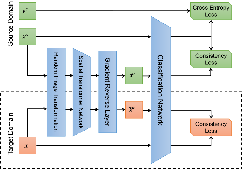
Figure 1: Overview of our proposed model. We propose to use random image transformations and adversarial spatial transformer networks (STN) to achieve domain adaptation and generalization (without the dash line bounding box).

Inspired by a recent line of work [13] [30] in semi-supervised learning which incorporates consistency training with unlabeled examples to enforce the smoothness of the model, we propose to use image transformation as a way of noisy injection and apply consistency training with the noisy and original examples. The overview of the proposed random image transformation with consistency training for domain adaptation is depicted in Figure 1. In this section, we focus on the random image transformation part and leave the adversarial spatial transformer networks in the next section. The main idea can be explained as follows:

(1) Given an input image ${\mathbf{x}}$ either from source or target domain, we compute the output distribution $p(y\mid{\mathbf{x}})$ with ${\mathbf{x}}$ and a noisy version $p(y\mid\tilde{{\mathbf{x}}})$ by applying random image transformation to ${\mathbf{x}}$;

(2) For domain adaptation, we jointly minimize the classification loss with labeled source domain samples and a divergence metric between the two distributions $\mathcal{D}(p(y\mid{\mathbf{x}})\parallel p(y\mid\tilde{{\mathbf{x}}}))$ with unlabeled source and target domain samples, where $\mathcal{D}$ is a discrepancy measure between two distributions;

(3) For domain generalization, the procedure is similar to (2) but without using any target domain samples.

Our intuition is that, on one hand, minimizing the consistency loss can enforce the model to be insensitive to the noise and improve the generalization ability; On the other hand, the consistency training gradually transmits label information from labeled source domain examples to unlabeled target domain ones, which improves the domain adaptation ability.

The applied random image transformations are similar to RandAugment [11]. Table 1 shows the types of image transformations used in this work. The images transformations are categorized into three groups. The first group is the geometric transformations, including Shear, Translation, Rotation and Flip. The second group is the color enhancing based image transformations, e.g. Solarize, Contrast etc., and the last group including other transformations e.g. CutOut and SamplePairing. Each type of image transformation has a corresponding magnitude, which indicates the strength of the transformation. The magnitude can be either a continues or discrete variable. Following [11], we also normalize the magnitude to a range from $0$ to $10$, in order to employ a linear scale of magnitude for each type of transformations. In other words, a value of $10$ indicates the maximum scale for a given transformation, while $0$ means minimum scale. Note that, these image transformations are commonly used as searching policies in recent auto-augmentation literatures, such as [9], [7] and [10]. Following [11], we do not use search, but instead uniformly sample from the same set of image transformations. Specifically, for each training sample, we uniformly sample $N_{aug}$ image transformations from Table 1 with normalized magnitude value of $M_{aug}$ and then apply them to the image sequentially. $N_{aug}$ and $M_{aug}$ are hyper-parameters. Following the practice of [11], we sampled $N_{aug}\in\{1,2,3,5,10\}$ and $M_{aug}\in\{3,6,9,12\}$. We conduct validation experiments on PACS dataset and VisDA dataset and find $N_{aug}=2$ and $M_{aug}=9$ obtains the best results, thus we keep $N_{aug}=2$ and $M_{aug}=9$ in all our experiments.

Following VAT [15] and UDA [13], we also use the KL divergence to compute the consistency loss. We denote by ${\bm{\theta}}_{m}$ the parameters of the classification model. The classification loss with labeled source domain samples is written as following cross entropy loss:

$$\mathcal{L}_{m}({\bm{\theta}}_{m})=\mathbb{E}_{{\mathbf{x}}^{s},\hat{y}^{s}\in\mathit{D}_{s}}[-\log{p(\hat{y}^{s}\mid{\mathbf{x}}^{s})}].$$ (1)

The consistency loss for domain adaptation can be written by:

$$\small\mathcal{L}_{c}({\bm{\theta}}_{m})=\mathbb{E}_{{\mathbf{x}}\in\mathit{D}_{s}\cup\mathit{D}_{t}}\mathbb{E}_{\tilde{{\mathbf{x}}}\in\tilde{\mathit{D}_{s}}\cup\tilde{\mathit{D}_{t}}}[\mathcal{D}_{\mathrm{KL}}(\hat{p}(y\mid{\mathbf{x}}),p(y\mid\tilde{{\mathbf{x}}}))],$$ (2)

where $\hat{p}(y\mid{\mathbf{x}})$ uses a fixed copy of ${\bm{\theta}}_{m}$ which means that the gradient is not propagated through $\hat{p}(y\mid{\mathbf{x}})$.

As a common underlying assumption in many semi-supervised learning methods, the classifier’s decision boundary should not pass through high-density regions of the marginal data distribution [51]. The conditional entropy minimization loss (EntMin) [52] enforces this by encouraging the classifier to output low-entropy predictions on unlabeled data. EntMin is also combined with VAT in [15] to obtain stronger results. Specifically, the conditional entropy minimization loss is written as:

$$\mathcal{L}_{e}({\bm{\theta}}_{m})=\mathbb{E}_{{\mathbf{x}}^{t}\in\mathit{D}_{t}}[-p(y^{t}\mid{\mathbf{x}}^{t})\log{p(y^{t}\mid{\mathbf{x}}^{t})}].$$ (3)

Following [6] and [5], we also apply the conditional entropy minimization loss to the unlabeled target domain data to minimize the classifier prediction uncertainty. The full objective of domain adaptation is thus written as follows:

$$\mathcal{J}_{DA}({\bm{\theta}}_{m})=\min_{{\bm{\theta}}_{m}}(\mathcal{L}_{m}+\lambda_{c}\mathcal{L}_{c}+\lambda_{e}\mathcal{L}_{e}),$$ (4)

where $\lambda_{c}$ and $\lambda_{e}$ are the weight factor for the consistency loss and conditional entropy minimization loss.

For domain generalization, as no target domain data is involved during the training, Equation 2 can be written as:

$$\small\mathcal{L}_{c}({\bm{\theta}}_{m})=\mathbb{E}_{{\mathbf{x}}\in\mathit{D}_{s}}\mathbb{E}_{\tilde{{\mathbf{x}}}\in\tilde{\mathit{D}_{s}}}[\mathcal{D}_{\mathrm{KL}}(\hat{p}(y\mid{\mathbf{x}}),p(y\mid\tilde{{\mathbf{x}}}^{t}))],$$ (5)

and the final objective function is the weighted sum of Equation 5 and the classification loss Equation 1 :

$$\mathcal{J}_{DG}({\bm{\theta}}_{m})=\min_{{\bm{\theta}}_{m}}(\mathcal{L}_{m}+\lambda_{c}\mathcal{L}_{c}).$$ (6)

Adversarial Spatial Transformer Networks

The proposed random image transformation with consistency training is a simple and effective method to reduce domain shift. Recent works show that using worst-case transformations or adversarial augmentation strategies can significantly improve the accuracy and robustness of the model [7] [8]. However, most of the image transformations in Section Random image transformation with consistency training are non-differentiable, making it difficult to apply gradient descent based method to obtain optimal transformations. To address this problem, searching algorithms such as reinforcement learning [7] or evolution strategy [8] are employed in recent works, which however are computationally expensive and don’t guarantee to obtain the global optima. In this work, we find that a subset of the image transformations in Table 1 are actually differentiable, i.e., the geometric transformations. In this work, we build our adversarial geometric transformation on top of the spatial transformer networks (STN) [16]. Specifically, in this work, we focus on the affine transformations. The STN consists of a localization network, a grid generator and a differentiable image sampler. The localization network is a convolutional neural network with parameter ${\bm{\theta}}_{t}$, it takes as input an image ${\mathbf{x}}$, and regress the affine transformation parameters ${\bm{\phi}}$. The grid generator takes as input ${\bm{\phi}}$, and generates the transformed pixel coordinates as follows:

$$\begin{bmatrix}u\\ v\end{bmatrix}={\bm{\phi}}\begin{bmatrix}\tilde{u}\\ \tilde{v}\\ 1\end{bmatrix}=\begin{bmatrix}\phi_{11}&\phi_{12}&\phi_{13}\\ \phi_{21}&\phi_{22}&\phi_{23}\end{bmatrix}\begin{bmatrix}\tilde{u}\\ \tilde{v}\\ 1\end{bmatrix},$$ (7)

where $(\tilde{u},\tilde{v})$ are the normalized transformed coordinates in the output image, $(u,v)$ are the normalized source coordinates in the input image, i.e., $-1\leq\tilde{u},\tilde{v},u,v\leq 1$. Finally, the differentiable image sampler takes the set of sampling points from the grid generator, along with the input image ${\mathbf{x}}$, and produces the sampled output image $\tilde{{\mathbf{x}}}$. The bilinear interpolation is used during the sampling process. We can denote STN by $\mathcal{T}:{\mathbf{x}}\rightarrow\tilde{{\mathbf{x}}}$ a differentiable neural network with parameter of ${\bm{\theta}}_{t}$, which applies an affine transformation to the input image ${\mathbf{x}}$.

The goal of the adversarial geometric transformation is to find the worst-case transformations, which is equivalent to maximize following objective function:

$$\operatornamewithlimits{argmax}_{{\bm{\theta}}_{t}}\mathbb{E}_{{\mathbf{x}}\in\mathit{D}_{s}\cup\mathit{D}_{t}}[\mathcal{D}_{\mathrm{KL}}(\hat{p}(y\mid{\mathbf{x}}),p(y\mid\mathcal{T}({{\mathbf{x}}}))].$$ (8)

The straightforward way to solve the maximization problem in Equation 8 is to apply the gradient reverse trick, i.e. the gradient reversal layer (GRL) in [2], which is popular in domain adversarial training methods. The GRL has no parameters associated with it. During the forward-propagation, it acts as an identity transformation. During the back-propagation however, the GRL takes the gradient from the subsequent level and changes its sign, i.e., multiplies it by $-1$, before passing it to the preceding layer. Formally, the forward and back-propagation of GRL can be written as $\mathcal{R}({\mathbf{x}})={\mathbf{x}},\frac{d\mathcal{R}}{d{\mathbf{x}}}=-\mathbf{I}$. The loss function of the adversarial spatial transformer for domain adaptation thus can be written by:

$$\small\mathcal{L}_{adv}({\bm{\theta}}_{t})=\mathbb{E}_{{\mathbf{x}}\in\mathit{D}_{s}\cup\mathit{D}_{t}}[\mathcal{D}_{\mathrm{KL}}(\hat{p}(y\mid{\mathbf{x}}),p(y\mid\mathcal{R}(\mathcal{T}({{\mathbf{x}}})))],$$ (9)

where $\mathcal{T}$ is the spatial transformer network with parameter ${\bm{\theta}}_{t}$, and $\mathcal{R}$ is the gradient reverse layer (GRL) [1]. For domain generalization, the only difference is that only ${\mathbf{x}}\in\mathit{D}_{s}$ is involved in Equation 9. With the adversarial spatial transformer network, the final objective function for domain adaptation is written by:

$$\begin{array}[]{c}\mathcal{J}_{DA}({\bm{\theta}}_{m},{\bm{\theta}}_{t})=\min_{{\bm{\theta}}_{m}}\max_{{\bm{\theta}}_{t}}(\mathcal{L}_{m}+\lambda_{c}\mathcal{L}_{c}+\\ \lambda_{e}\mathcal{L}_{e}+\lambda_{t}\mathcal{L}_{adv}),\\ \end{array}$$ (10)

and the final objective function for domain generalization is written by:

$$\small\begin{array}[]{c}\mathcal{J}_{DG}({\bm{\theta}}_{m},{\bm{\theta}}_{t})=\min_{{\bm{\theta}}_{m}}\max_{{\bm{\theta}}_{t}}(\mathcal{L}_{m}+\lambda_{c}\mathcal{L}_{c}+\lambda_{t}\mathcal{L}_{adv}).\end{array}$$ (11)

Experiments

In this section, we conduct experiments to evaluate the proposed method and compare the results with the state-of-the-art domain adaptation and generalization methods.

Methods	Task	Year	Description
DANN [22]	DA	2015	Domain adversarial training.
DAN [1]	DA	2015	Deep adaptation network.
ADDA [3]	DA	2017	Adversarial discriminative domain adaptation.
JAN [53]	DA	2017	Joint adaptation network.
Dial [54]	DA	2017	Domain alignment layers.
DDiscovery [55]	DA	2018	Domain discovery.
CDAN [56]	DA	2018	Conditional domain adversarial training.
MDD [57]	DA	2019	Adversarial training with margin disparity discrepancy.
Rot [5]	DA	2019	Self-supervised learning by rotation prediction.
RotC [30]	DA	2020	Self-supervised learning with consistency training.
ALDA [29]	DA	2020	Adversarial-learned loss for domain adaptation.
MLADA [25]	DA	2021	Multi-layer adversarial domain adaptation.
GPDA [58]	DA	2021	Geometrical preservation and distribution alignment.
CCSA [59]	DA & DG	2017	Embedding subspace learning.
JiGen [6]	DA & DG	2019	Self-supervised learning by solving jigsaw puzzle.
JigRot [43]	DA & DG	2021	Self-supervised learning by combining jigsaw and rotation.
TF [60]	DG	2017	Low-rank parametrized network.
SLRC [38]	DG	2017	Low rank constraint.
CIDDG [61]	DG	2018	Conditional invariant deep domain generalization.
MMD-AAE [33]	DG	2018	Adversarial auto-encoders.
D-SAM [62]	DG	2018	Domain-specific aggregation modules.
MLDG [40]	DG	2018	Meta learning approach.
MetaReg [39]	DG	2018	Meta learning approach.
MMLD [63]	DG	2020	Mixture of Multiple Latent Domains.
ER [64]	DG	2020	Domain generalization via entropy regularization.
DADG [42]	DG	2021	Discriminative adversarial domain generalization.
WADG [35]	DG	2021	Wasserstein adversarial domain generalization.

Table 2: The compared state-of-the-art methods on domain adaptation (DA) and domain generalization (DG) task. The column Year shows the published year of each method.

Datasets

Our method is evaluated on the following popular domain adaptation and generalization datasets:

PACS [60] is a standard dataset for DG. It contains $9991$ images collected from Sketchy, Caltech256, TU-Berlin and Google Images. It has $4$ domains (Photo, Art Paintings, Cartoon and Sketches) and each domain consists of $7$ object categories. Following [6], we evaluate both domain generalization and multi-source domain adaptation on this dataset.

ImageCLEF-DA [65] is a benchmark dataset in the domain adaptation community for the ImageCLEF 2014 domain adaptation challenge. It consists of three domains, including Caltech-256 (C), ImageNet ILSVRC 2012 (I), and Pascal VOC 2012 (P). Each domain consist of $12$ common classes. Six domain adaptation tasks are evaluated on ImageCLEF: $\textbf{I}\rightarrow\textbf{P}$, $\textbf{P}\rightarrow\textbf{I}$, $\textbf{I}\rightarrow\textbf{C}$, $\textbf{C}\rightarrow\textbf{I}$, $\textbf{C}\rightarrow\textbf{P}$ and $\textbf{P}\rightarrow\textbf{C}$. There are $600$ images in each domain and $50$ images in each category.

Office-Home [66] is used for evaluating both domain adaptation and generalization. It contains 4 domains and each domain consists of images from 65 categories of everyday objects. The 4 domains are: Art (A), Clipart (C), Product (P) and Real-World (R). The Clipart domain is formed with clipart images. The Art domain consists of artistic images in the form of paintings, sketches, ornamentation etc.. The Real-world domain’s images are captured by a regular camera and the Product domain’s images have no background. The total number of images is about $15500$.

VLCS [67] is used for evaluating domain generalization. It contains images of $5$ object categories shared by $4$ separated domains: PASCAL VOC 2007, LabelMe, Caltech and Sun datasets. Different from Office-Home and PACS which are related in terms of domain types, VLCS offers different challenges because it combines object categories from Caltech with scene images of the other domains.

VisDA is a simulation-to-real domain adaptation dataset, which has over $280K$ images across $12$ classes. The synthetic domain contains renderings of 3D models from different angles and with different lighting conditions, and the real domain contains nature images.

To investigate the robustness of the proposed model, we also evaluate on popular robustness benchmarks, including:

CIFAR-10.1 [68] is a new test set of CIFAR-10 with $2000$ images and the exact same classes and image dimensionality. Its creation follows the creation process of the original CIFAR-10 paper as closely as possible. The purpose of this dataset is to investigate the distribution shifts present between the two test sets, and the effect on object recognition.

CIFAR-10-C [17] is a robustness benchmark where $15$ types of corruption are algorithmically simulated to mimic real-world corruption as much as possible on copies of the CIFAR-10 [69] test set. The $15$ types of corruption are from four broad categories: noise, blur, weather and digital. Each corruption type comes in five levels of severity, with level 5 the most severe. In this work, we evaluate with the level 5 severity.

Experimental Setting

We implement the proposed method using the PyTorch framework on a single RTX 2080 Ti GPU with $11$ GB memory. Alexnet [70], Resnet-18 and Resnet-50 [71] architectures are used as base networks and initialized with ImageNet [72] pretrained weights.

For training the model, we use an SGD solver with an initial learning rate of $0.001$. We train the model for $60$ epochs and decay the learning rate to $0.0001$ after $80\%$ of the training epochs. For training baseline models, we use simple data augmentation protocols by random cropping, horizontal flipping and color jittering.

We follow the standard protocol for unsupervised domain adaptation [22] and [53] where all labeled source domain examples and all unlabeled target domain examples are used for adaptation tasks. We also follow the standard protocol for domain generalization transfer tasks as [6] where the target domain examples are unavailable in the training phase. We set three different random seeds and run each experiment three times. The final result is the average over the three repetitions.

We compare our proposed method with state-of-the-art DA and DG methods. The descriptions of the compared methods are shown in Table 2. In the following, we use Deep All to denote the baseline model trained with all available source domain examples when all the introduced domain adaptive conditions are disabled. For the compared methods in Table 2, we use the results reported from the original papers if the protocol is the same.

Experimental Results

Unsupervised domain adaptation

The multiple source domain adaptation results on PACS are reported in Table 3. We follow the settings in [6] and [5] and trained our model considering three domains as source datasets and the remaining one as target. RotC is an improved version Rot, which applies consistency loss with the simplest image rotation transformations [30]. We use the open source of [56] to produce the results of CDAN and CDAN+E and the open source of [57] to produce the results of MDD. Our proposed approach outperforms all baseline methods on all transfer tasks. The last column shows the average accuracy on the $4$ tasks. Our proposed approach outperforms state-of-the-art CDAN+E [56] by $4.7$ percentage points and MDD by $1.4$ percentage point.

To investigate the improvement from data augmentation, we add the same type of data augmentation as ours on Deep All, DANN, CDAN, CDAN+E and MDD, which are denoted by Deep All (Aug), DANN (Aug), CDAN (Aug), CDAN+E (Aug) and MDD (Aug). From these results, we can see that data augmentation can obtain $1.2$ to $2.6$ percentage point improvement for existing domain adaptation methods. Even with the same type of data augmentation, our proposed method still outperforms these baselines.

PACS-DA		art_paint.	cartoon	sketches	photo	Avg.
[55]	Deep All	74.70	72.40	60.10	92.90	75.03
	Dial	87.30	85.50	66.80	97.00	84.15
	DDiscovery	87.70	86.90	69.60	97.00	85.30
[6]	Deep All	77.85	74.86	67.74	95.73	79.05
	JiGen	84.88	81.07	79.05	97.96	85.74
[5]	Deep All	74.70	72.40	60.10	92.90	75.00
	Rot	88.70	86.40	74.90	98.00	87.00
[30]	Deep All	74.70	72.40	60.10	92.90	75.00
	RotC	90.30	87.40	75.10	97.90	87.70
[43]	Deep All	77.83	74.26	65.81	95.71	78.40
	JigRot	89.67	82.87	83.93	98.17	88.66
[56]	DANN	82.91	83.83	69.50	96.29	83.13
	DANN (Aug)	89.01	83.06	78.54	97.25	86.96
[56]	CDAN	85.70	88.10	73.10	97.20	86.00
	CDAN+E	87.40	89.40	75.30	97.80	87.50
	CDAN (Aug)	90.67	85.96	80.50	97.43	88.64
	CDAN+E (Aug)	90.28	85.41	81.37	98.08	88.78
[57]	MDD	89.60	88.99	87.35	97.78	90.92
	MDD (Aug)	90.28	86.26	85.72	97.54	89.95
	Deep All	77.26	72.64	69.05	95.41	78.59
	Deep All (Aug)	80.03	74.49	67.85	95.27	79.41
	Ours	92.56	91.44	87.08	98.04	92.28

Table 3: Multi-source domain adaptation results on PACS (Reset-18). Each column title indicates the name of the domain used as target. We use the bold font to highlight the best results.

The results on Office-Home dataset are reported in Table 4. On Office-Home dataset, we conducted $12$ transfer tasks of $4$ domains in the context of single source domain adaptation. We achieve state-of-the-art performance on $8$ out of $12$ transfer tasks. It is noted that although Office-Home and PACS are related in terms of domain types, the number of total categories in Office-Home and PACS are $65$ and $7$ respectively. From the results, we can see that the proposed method scales when the number of categories changes from $7$ to $65$. The average accuracy achieved by our proposed method is $67.6\%$ which outperforms all the compared methods.

Office-Home	$\textbf{A}\xrightarrow{}\textbf{C}$	$\textbf{A}\xrightarrow{}\textbf{P}$	$\textbf{A}\xrightarrow{}\textbf{R}$	$\textbf{C}\xrightarrow{}\textbf{A}$	$\textbf{C}\xrightarrow{}\textbf{P}$	$\textbf{C}\xrightarrow{}\textbf{R}$	$\textbf{P}\xrightarrow{}\textbf{A}$	$\textbf{P}\xrightarrow{}\textbf{C}$	$\textbf{P}\xrightarrow{}\textbf{R}$	$\textbf{R}\xrightarrow{}\textbf{A}$	$\textbf{R}\xrightarrow{}\textbf{C}$	$\textbf{R}\xrightarrow{}\textbf{P}$	Avg.
ResNet-50 [71]	34.9	50.0	58.0	37.4	41.9	46.2	38.5	31.2	60.4	53.9	41.2	59.9	46.1
DAN [1]	43.6	57.0	67.9	45.8	56.5	60.4	44.0	43.6	67.7	63.1	51.5	74.3	56.3
DANN [22]	45.6	59.3	70.1	47.0	58.5	60.9	46.1	43.7	68.5	63.2	51.8	76.8	57.6
JAN [53]	45.9	61.2	68.9	50.4	59.7	61.0	45.8	43.4	70.3	63.9	52.4	76.8	58.3
GPDA [58]	52.9	73.4	77.1	52.9	66.1	65.6	52.9	44.9	76.1	65.6	49.7	79.2	63.0
CDAN [56]	49.0	69.3	74.5	54.4	66.0	68.4	55.6	48.3	75.9	68.4	55.4	80.5	63.8
Rot [5]	50.4	67.8	74.6	58.7	66.7	67.4	55.7	52.4	77.5	71.0	59.6	81.2	65.3
CDAN+E [56]	50.7	70.6	76.0	57.6	70.0	70.0	57.4	50.9	77.3	70.9	56.7	81.6	65.8
ALDA [29]	53.7	70.1	76.4	60.2	72.6	71.5	56.8	51.9	77.1	70.2	56.3	82.1	66.6
RotC [30]	51.7	69.0	75.4	60.4	70.3	70.7	57.7	53.3	78.6	72.2	59.9	81.7	66.7
Ours	55.1	69.0	74.5	62.5	66.7	69.8	62.2	56.0	77.7	73.5	61.9	82.2	67.6

Table 4: Accuracy (%) on Office-Home for unsupervised domain adaptation (Resnet-50). The bold font highlights the best domain adaptation results. $\textbf{A}\xrightarrow{}\textbf{C}$ indicates A (Art) is the source domain and C (Clipart) is the target domain.

The results on ImageCLEF-DA dataset are reported in Table 5. As the three domains in ImageCLEF-DA are of equal size and balanced in each category, and are visually more similar, there is little room of improvement in this dataset. Even though, our method still outperforms the comparison methods on $4$ out of $6$ transfer tasks. Our method achieved $88.2\%$ average accuracy, outperforming the latest methods including CDAN+E [56], RotC [30] and MLADA [25].

ImageCLEF-DA	$\textbf{I}\rightarrow\textbf{P}$	$\textbf{P}\rightarrow\textbf{I}$	$\textbf{I}\rightarrow\textbf{C}$	$\textbf{C}\rightarrow\textbf{I}$	$\textbf{C}\rightarrow\textbf{P}$	$\textbf{P}\rightarrow\textbf{C}$	Avg.
ResNet-50 [71]	74.8	83.9	91.5	78.0	65.5	91.2	80.7
DAN [1]	74.5	82.2	92.8	86.3	69.2	89.8	82.5
Rot [5]	77.9	91.6	95.6	86.9	70.5	94.8	84.2
DANN [22]	75.0	86.0	96.2	87.0	74.3	91.5	85.0
JAN [53]	76.8	88.0	94.7	89.5	74.2	91.7	85.8
CDAN [56]	76.7	90.6	97.0	90.5	74.5	93.5	87.1
MLADA [25]	78.2	91.2	95.5	90.8	76.0	92.2	87.3
CDAN+E [56]	77.7	90.7	97.7	91.3	74.2	94.3	87.7
RotC [30]	78.6	92.5	96.1	88.9	73.9	95.9	87.7
Ours	78.1	92.7	96.5	91.6	74.9	95.9	88.2

Table 5: Accuracy (%) on ImageCLEF-DA for unsupervised domain adaptation (Resnet-50). The bold font highlights the best domain adaptation results. $\textbf{I}\rightarrow\textbf{P}$ indicates ImageNet ILSVRC 2012 is source domain and Pascal VOC 2012 is target domain.

The proposed method also obtains strong results on VisDA as reported in Table 6. It outperforms CDAN+E by $2.6$ percentage points.

Method	Accuracy
JAN [53]	61.6
GTA [73]	69.5
CDAN [56]	66.8
CDAN+E [56]	70.0
Ours	72.6

Table 6: Accuracy (%) on VisDA (Synthetic $\rightarrow$ Real) for unsupervised domain adaptation (ResNet-50).

It is important to understand the improvement of the consistency loss. Because RotC is the combination of simple image rotation transformation and consistency loss, without using complex data augmentation, we can better understand how much improvement is from the consistency loss. Comparing to Rot, which does not use consistency loss, we can see from the above DA experiments that RotC obtains about $0.7$ to $3.5$ percentage points improvement thanks to the consistency loss.

Domain generalization

In the context of multi-source domain generalization, we conduct $4$ transfer tasks on PACS dataset. We compare the performance of our proposed method against several recent domain generalization methods. We evaluated with both Alexnet and Resnet-18 and report the results in Table 7 and Table 8. From the results, we can observe that our proposed method achieves state-of-the-art domain generalization performance with both backbone architectures. With Alexnet, our method outperforms the comparison methods on all $4$ transfer tasks. The average accuracy of our method outperforms the prior best method WADG by around $1.7$ percentage points, setting a new state-of-the-art performance. With Resnet-18, the average accuracy of our method is $82.73\%$, also outperforming the existing latest ones.

As the consistency loss is not mandatory for DG, we replace consistency loss by the cross-entropy loss and run our methods. The results are denoted by Ours w/o consis.. We can see that the model trained with cross-entropy loss obtains similar accuracy to ours with consistency loss. However, the consistency loss is required for DA because of the unlabeled target domain samples. To keep a unified framework for both DA and DG problems, we use consistency loss for DG in this work.

To investigate the improvement of pure data augmentation without consistency. We run JiGen and Deep All with the same type of data augmentation as ours, denoted by JiGen (Aug) and Deep All (Aug). We can see that using pure augmentation, Deep All can obtain around $0.8$ to $1.2$ percentage point improvement, JiGen can obtain around $1.2$ to $1.6$ percentage point improvement. Even though, our proposed method still outperforms these baselines.

PACS-DG		art_paint.	cartoon	sketches	photo	Avg.
[60]	Deep All	63.30	63.13	54.07	87.70	67.05
	TF	62.86	66.97	57.51	89.50	69.21
[61]	Deep All	57.55	67.04	58.52	77.98	65.27
	DeepC	62.30	69.58	64.45	80.72	69.26
	CIDDG	62.70	69.73	64.45	78.65	68.88
[40]	Deep All	64.91	64.28	53.08	86.67	67.24
	MLDG	66.23	66.88	58.96	88.00	70.01
[62]	Deep All	64.44	72.07	58.07	87.50	70.52
	D-SAM	63.87	70.70	64.66	85.55	71.20
[42]	Deep All	63.12	66.16	60.27	88.65	69.55
	DADG	66.21	70.28	62.18	89.76	72.11
[39]	Deep All	67.21	66.12	55.32	88.47	69.28
	MetaReg	69.82	70.35	59.26	91.07	72.63
[6]	Deep All	66.68	69.41	60.02	89.98	71.52
	JiGen	67.63	71.71	65.18	89.00	73.38
	JiGen (Aug)	71.53	69.50	68.06	91.08	75.04
[43]	Deep All	66.50	69.65	61.42	89.68	71.81
	JigRot	69.70	71.00	66.00	89.60	74.08
[63]	Deep All	68.09	70.23	61.80	88.86	72.25
	MMLD	69.27	72.83	66.44	88.98	74.38
[64]	Deep All	68.35	70.14	90.83	64.98	73.57
	ER	71.34	70.29	89.92	71.15	75.67
[35]	Deep All	63.30	63.13	54.07	87.70	67.05
	WADG	70.21	72.51	70.32	89.81	75.71
	Deep All	68.26	74.52	63.65	90.78	74.30
	Deep All (Aug)	73.73	70.09	65.79	92.22	75.45
	Ours w/o consis.	73.44	71.42	73.91	89.70	77.12
	Ours	74.02	72.23	72.36	91.16	77.44

Table 7: Domain generalization results on PACS (Alexnet). For details about meaning of columns and use of bold fonts, see Table 3.

PACS-DG		art_paint.	cartoon	sketches	photo	Avg.
[42]	Deep All	75.60	72.30	68.10	93.06	77.27
	DADG	79.89	76.25	70.51	94.86	80.38
[62]	Deep All	77.87	75.89	69.27	95.19	79.55
	D-SAM	77.33	72.43	77.83	95.30	80.72
[6]	Deep All	77.85	74.86	67.74	95.73	79.05
	JiGen	79.42	75.25	71.35	96.03	80.51
	JiGen (Aug)	79.44	71.50	70.86	95.33	79.28
[64]	Deep All	78.93	75.02	96.60	70.48	80.25
	ER	80.70	76.40	96.65	71.77	81.38
[43]	Deep All	77.83	74.26	65.81	95.71	78.40
	JigRot	81.07	73.97	74.67	95.93	81.41
[39]	Deep All	79.90	75.10	69.50	95.20	79.93
	MetaReg	83.70	77.20	70.30	95.50	81.68
[63]	Deep All	78.34	75.02	65.24	96.21	78.70
	MMLD	81.28	77.16	72.29	96.09	81.83
	Deep All	77.26	72.64	69.05	95.41	78.59
	Deep All (Aug)	80.03	74.49	67.85	95.27	79.41
	Ours w/o consis.	81.84	75.05	77.01	95.07	82.24
	Ours	82.32	75.70	77.03	95.87	82.73

Table 8: Domain generalization results on PACS (Resnet-18). For details about meaning of columns and use of bold fonts, see Table 3.

We also conduct experiments on Office-Home and VLCS dataset for multi-source domain generalization. Compare to PACS, these two datasets are more difficult and most of the recent works have only obtained small accuracy gain with respect to the Deep All baselines. The results on Office-Home and VLCS dataset are reported in Table 9 and Table 10 respectively. Our proposed method outperforms the comparison methods on the four transfer tasks on Office-Home dataset. And the results tested on VLCS dataset show that our method achieve the best or close to the best performance on the four tasks, outperforming the recently proposed ones in average. It is noted that our baseline Deep All has relatively higher accuracy than other baselines. This is because we also add data augmentations such as random crop, horizontal flipping and color jittering when training Deep All models. In this case, it is fairer to compare with the proposed method which incorporates various data augmentation operations.

Office-Home-DG		Art	Clipart	Product	Real-World	Avg.
[62]	Deep All	55.59	42.42	70.34	70.86	59.81
	D-SAM	58.03	44.37	69.22	71.45	60.77
	Deep All	52.15	45.86	70.86	73.15	60.51
[6]	JiGen	53.04	47.51	71.47	72.79	61.20
[35]	WADG	55.34	44.82	72.03	73.55	61.44
[43]	JigRot	58.33	49.67	72.97	75.27	64.06
[42]	Deep All	54.31	41.41	70.31	73.03	59.77
	DADG	55.57	48.71	70.90	73.70	62.22
	Deep All	57.16	49.06	72.22	73.59	63.01
	Ours	59.20	54.67	73.21	73.93	65.25

Table 9: Domain generalization results on Office-Home (Resnet-18). For details about meaning of columns and use of bold fonts, see Table 3.

VLCS-DG		Caltech	Labelme	Pascal	Sun	Avg.
[61]	Deep All	85.73	61.28	62.71	59.33	67.26
	DeepC	87.47	62.60	63.97	61.51	68.89
	CIDDG	88.83	63.06	64.38	62.10	69.59
[59]	Deep All	86.10	55.60	59.10	54.60	63.85
	CCSA	92.30	62.10	67.10	59.10	70.15
[38]	Deep All	86.67	58.20	59.10	57.86	65.46
	SLRC	92.76	62.34	65.25	63.54	70.97
[60]	Deep All	93.40	62.11	68.41	64.16	72.02
	TF	93.63	63.49	69.99	61.32	72.11
[33]	MMD-AAE	94.40	62.60	67.70	64.40	72.28
[62]	Deep All	94.95	57.45	66.06	65.87	71.08
	D-SAM	91.75	56.95	58.59	60.84	67.03
[43]	Deep All	96.15	59.05	70.84	63.92	72.49
	JigRot	96.30	59.20	70.73	66.37	73.15
[6]	Deep All	96.93	59.18	71.96	62.57	72.66
	JiGen	96.93	60.90	70.62	64.30	73.19
[63]	Deep All	95.89	57.88	72.01	67.76	73.39
	MMLD	96.66	58.77	71.96	68.13	73.88
[64]	Deep All	97.15	58.07	73.11	68.79	74.28
	ER	96.92	58.26	73.24	69.10	74.38
[35]	Deep All	92.86	63.10	68.67	64.11	72.19
	WADG	96.68	64.26	71.47	66.62	74.76
[42]	Deep All	94.44	61.30	68.11	63.58	71.86
	DADG	96.80	63.44	70.77	66.81	74.76
	Deep All	97.72	63.03	71.93	66.70	74.85
	Ours	98.74	62.27	72.79	68.16	75.49

Table 10: Domain generalization results on VLCS (Alexnet). For details about meaning of columns and use of bold fonts, see Table 3.

Robustness

Apart from domain adaptation and generalization, we are also interested in the robustness of the learned model. In this part, we evaluate the proposed method on robustness benchmarks CIFAR-10.1 and CIFAR-10-C. We train on the standard CIFAR-10 training set and test on various corruption datasets, i.e., in a single source domain generalization setting. Figure 2 shows the testing error on different datasets. We evaluate different image transform strategies and also compare to recently proposed methods in [74], i.e., JT and TTT. Following [74], we use the same architecture and hyper-parameters across all experiments.

The method denoted by baseline refers to the plain Resnet model which is equivalent to Deep All in DG setting. JT and TTT are the joint training and testing time training in [74] respectively. We denote by rnd-all the random image transformation including geometric and color-based transformations, adv-stn the proposed adversarial STN without random image transforms and adv-stn-color the adversarial STN combined with random color-based transformations.

On the leftmost, it is the standard CIFAR-10 testing dataset, where we can see that all the compared methods have obtained similar accuracies. On CIFAR10.1, the testing errors of all these methods increase simultaneously, but there is no significant gap between them. On CIFAR-10-C corruption data sets, the performances of these methods vary a lot. Our proposed methods show improved accuracies comparing to the baseline. adv-stn-color shows better performance than its variants and also outperforms JT and TTT. It can also be seen that adv-stn even outperforms rnd-all in most cases, although it only applies geometric transformations, which indicates the effectiveness of the proposed adversarial spatial transformations for improving robustness.

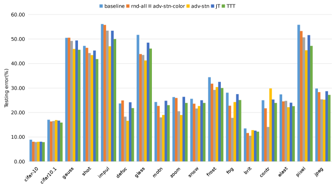
Figure 2: Test error (%) on CIFAR-10, CIFAR10.1 and CIFAR-10-C (level 5). Best viewed in color.

Ablation Studies and Analysis

We focus on the PACS DG and DA setting for an ablation analysis on the proposed method.

Ablation study on image transformation strategies

In this part, we conduct ablation studies on adversarial and random image transformations. Table 11 shows the ablation studies of domain adaptation on PACS with different image transformation strategies, and Table 12 shows the domain generalization results. rnd-color and rnd-geo are subsets of rnd-all, where rnd-color refers to color-based transformations and rnd-geo refers to geometric transformations. Please see Table 1 for details of each subset of transformations. For DA task, when comparing individual transformation strategies, rnd-color obtained best accuracy and adv-stn outperforms rnd-geo. The combination of rnd-color + adv-stn also outperforms rnd-color + rnd-geo. However, in this experiment adv-stn does not further improve rnd-color, which might due to the limited room for improvement of the baseline method.

PACS-DA
rnd-color	rnd-geo	adv-stn	art_paint.	cartoon	sketches	photo	Avg.
$\surd$			93.02	91.51	86.62	98.00	92.29
	$\surd$		91.83	89.45	83.42	97.98	90.67
		$\surd$	91.85	91.61	82.45	97.92	90.96
$\surd$	$\surd$		93.10	91.01	86.33	98.14	92.15
$\surd$		$\surd$	92.56	91.44	87.08	98.04	92.28

Table 11: Ablation studies of domain adaptation on PACS. The first three columns indicate the types of image transformations applied. Each column title in the middle indicates the name of the domain used as target. We use the bold font to highlight the best results.

PACS-DG
rnd-color	rnd-geo	adv-stn	art_paint.	cartoon	sketches	photo	Avg.
$\surd$			71.40	72.43	71.44	90.20	76.37
	$\surd$		71.08	72.40	66.98	91.36	75.46
		$\surd$	70.92	73.46	69.66	90.78	76.21
$\surd$	$\surd$		73.05	72.15	69.08	91.64	76.48
$\surd$		$\surd$	74.02	72.23	72.36	91.16	77.44

Table 12: Ablation studies of domain generalization on PACS. The first three columns indicate the types of image transformations applied. Each column title in the middle indicates the name of the domain used as target. We use the bold font to highlight the best results.

In the DG experiment, we get similar conclusion that adv-stn outperforms rnd-geo. As the baseline accuracy of DG is far from saturated than DA, we can see that adv-stn further improves rnd-color and the combination of rnd-color + adv-stn obtained the best accuracy.

Ablation study on hyperparameters setting

In this part, we conduct ablation studies on hyperparameters setting. The final objective functions of our proposed method for domain adaptation (10) and domain generalization (11) are weighted summation of several items, with the weighting factors as the hyperparameters. Since the conditional entropy minimization loss is widely used domain adaptation, we fixed the weight $\lambda_{e}=0.1$ and conducted grid test with different settings of $\lambda_{c}$ and $\lambda_{t}$, which are shared by domain generalization. We tested ten different values which are logarithmically spaced between $10^{-2}$ and $10$ for $\lambda_{c}$ and $\lambda_{t}$. For each setting, we run with three different random seeds and calculate the mean accuracy. The results of multi-source domain adaptation and domain generalization which take photo, cartoon and sketch as the source domains and art_painting as the target domain are reported in Figure 3. Resnet-18 is used as the base network.

From the figures, we can see that when both $\lambda_{c}$ and $\lambda_{t}$ are not too large, the accuracies are relatively stable, validating the insensitiveness of our proposed method to hyperparameters. However, when $\lambda_{c}$ and $\lambda_{t}$ grow too large, the performance decreases, especially with a small $\lambda_{c}$ and a large $\lambda_{t}$. The reason maybe that overwhelmingly large weights for consistency loss and adversarial spatial transformer loss over the main classification loss make the learned feature less discriminative for the main classification task, therefore resulting in lower accuracy. And too large $\lambda_{t}$ may lead to excessive emphasis on the extreme geometric distortions, which may be harmful to the general cross domain performance.

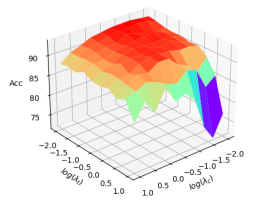
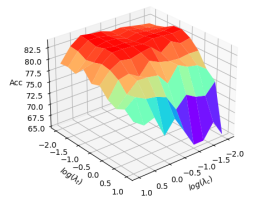
(a)	(b)

Figure 3: Accuracies with different hyperparameter settings on PACS $\textbf{photo},\textbf{cartoon},\textbf{sketch}\rightarrow{}\textbf{art\_painting}$ task (Resnet-18). (a) Multi-source Domain adaptation with fixed $\lambda_{e}$. (b) Domain generalization. Best viewed in color.

Visualization of learned deep features

To better understand the learned domain invariant feature representations, we use t-SNE [75] to conduct an embedding visualization. We conduct experiments on transfer task of $\textbf{photo},\textbf{cartoon},\textbf{sketch}\rightarrow{}\textbf{art\_painting}$ with both DA and DG settings and visualize the feature embeddings. Figure4 shows the visualization on PACS DA setting, and Figure5 shows the visualization on PACS DG setting. On both figures, we visualize category alignment as well as domain alignment. We also compare to the baseline Deep All which does not apply any adaptation.

From the visualization of the embeddings, we can see that the clusters created by our model not only separates the categories but also mixes the domains. The visualization from DG model suggests that our proposed method is able to learn feature representations generalizable to unseen domains. It also implies that the proposed method can effectively learn domain invariant representation with unlabeled target domain examples.

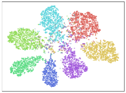
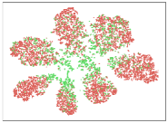
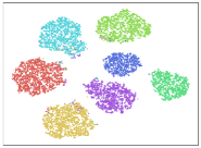
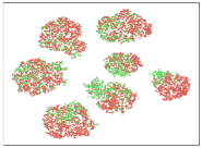
(a)	(b)	(c)	(d)

Figure 4: The t-SNE visualization on the PACS DA setting: (a) class visualization of Deep All, (b) domain visualization of Deep All, (c) class visualization of Ours, (d) domain visualization of Ours.

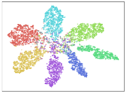
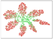
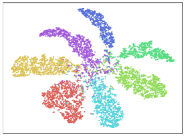
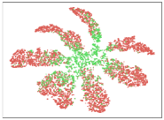
(a)	(b)	(c)	(d)

Figure 5: The t-SNE visualization on the PACS DG setting: (a) class visualization of Deep All, (b) domain visualization of Deep All, (c) class visualization of Ours, (d) domain visualization of Ours.

Visualization of adversarial examples

To visually examine what are the adversarial spatial transformations learned by adv-stn, we plot the transformed examples during training in Figure 6. In the first row, we show the original images with simple random horizontal flipping and jittering augmentation. The second and third rows show images with rnd-all and adv-stn-color respectively. From the figure, we can see that the proposed adversarial STN does find more difficult image transformations than the random augmentation. Training with these adversarial examples greatly improves the generalization ability and robustness of the model.

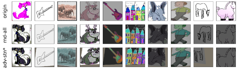
Figure 6: Visualization of the transformed images during the PACS DG training. First row: original image with random horizontal flipping and jittering; second row: original image with the proposed random augmentation; third row: the original image with the proposed adversarial spatial transformation combined with random color-based transformations.

Conclusion

In this work, we proposed a unified framework for addressing both domain adaptation and generalization problems. Our domain adaptation and generalization methods are built upon random image transformation and consistency training. This simple strategy can obtain promising DA and DG performance on multiple benchmarks. To further improve its performance, we proposed a novel adversarial spatial transformer networks which can find the worst-case image transformation to improve the generalizability and robustness of the model. Experimental results on multiple object recognition DA and DG benchmarks verified the effectiveness of the proposed methods.

References

- [1] Mingsheng Long, Yue Cao, Jianmin Wang and Michael I Jordan. “Learning transferable features with deep adaptation networks”. In Int. Conf. on Machine Learning, 2015.
- [2] Yaroslav Ganin, Evgeniya Ustinova, Hana Ajakan et al. “Domain-adversarial training of neural networks”. Journal of Machine Learning Research, vol. 17, no. 1, 2096–2030, January 2016.
- [3] Eric Tzeng, Judy Hoffman, Kate Saenko and Trevor Darrell. “Adversarial discriminative domain adaptation”. In IEEE Conf. on Computer Vision and Pattern Recognition, 2017.
- [4] Judy Hoffman, Eric Tzeng, Taesung Park et al. “Cycada: Cycle consistent adversarial domain adaptation”. In Int. Conf. on Machine Learning, 2018.
- [5] J. Xu, L. Xiao and A. M. López. “Self-supervised domain adaptation for computer vision tasks”. IEEE Access, vol. 7, 156694–156706, 2019.
- [6] Fabio Maria Carlucci, Antonio D’Innocente, Silvia Bucci, Barbara Caputo and Tatiana Tommasi. “Domain generalization by solving jigsaw puzzles”. In IEEE Conf. on Computer Vision and Pattern Recognition, 2019.
- [7] Xinyu Zhang, Qiang Wang, Jian Zhang and Zhao Zhong. “Adversarial autoaugment”. In Int. Conf. on Learning Representations, 2020.
- [8] Riccardo Volpi and Vittorio Murino. “Addressing model vulnerability to distributional shifts over image transformation sets”. In Int. Conf. on Computer Vision, 2019.
- [9] Ekin D. Cubuk, Barret Zoph, Dandelion Mane, Vijay Vasudevan and Quoc V. Le. “Autoaugment: Learning augmentation policies from data”. In IEEE Conf. on Computer Vision and Pattern Recognition, June 2019.
- [10] Sungbin Lim, Ildoo Kim, Taesup Kim, Chiheon Kim and Sungwoong Kim. “Fast autoaugment”. In Advances in Neural Information Processing Systems, 2019.
- [11] Ekin D. Cubuk, Barret Zoph, Jonathon Shlens and Quoc V. Le. “Randaugment: Practical data augmentation with no separate search”. In Advances in Neural Information Processing Systems, 2020.
- [12] Mehdi Sajjadi, Mehran Javanmardi and Tolga Tasdizen. “Regularization with stochastic transformations and perturbations for deep semi-supervised learning”. In Advances in Neural Information Processing Systems, 2016.
- [13] Qizhe Xie, Zihang Dai, Eduard Hovy, Thang Luong and Quoc Le. “Unsupervised data augmentation for consistency training”. In Advances in Neural Information Processing Systems, 2020.
- [14] Teppei Suzuki and Ikuro Sato. “Adversarial Transformations for Semi-Supervised Learning”. In AAAI, 2020.
- [15] Takeru Miyato, Shin-Ichi Maeda, Masanori Koyama and Shin Ishii. “Virtual adversarial training: A regularization method for supervised and semi-supervised learning”. IEEE Trans. on Pattern Analysis and Machine Intelligence, vol. 41, no. 8, 1979–1993, 2019.
- [16] Max Jaderberg, Karen Simonyan, Andrew Zisserman et al. “Spatial transformer networks”. In Advances in Neural Information Processing Systems, pages 2017–2025, 2015.
- [17] Dan Hendrycks and Thomas Dietterich. “Benchmarking neural network robustness to common corruptions and perturbations”. In Int. Conf. on Learning Representations, 2019.
- [18] Eric Tzeng, Judy Hoffman, Ning Zhang, Kate Saenko and Trevor Darrell. “Deep domain confusion: Maximizing for domain invariance”. In IEEE Conf. on Computer Vision and Pattern Recognition, 2014.
- [19] Ke Wang, Jiayong Liu and Jing-Yan Wang. “Learning domain-independent deep representations by mutual information minimization”. Computational Intelligence and Neuroscience, vol. 2019, 2019.
- [20] Baochen Sun, Jiashi Feng and Kate Saenko. “Return of frustratingly easy domain adaptation”. In AAAI, 2016.
- [21] Baochen Sun and Kate Saenko. “Deep CORAL: Correlation alignment for deep domain adaptation”. In European Conf. on Computer Vision, 2016.
- [22] Yaroslav Ganin and Victor Lempitsky. “Domain-Adversarial Training of Neural Networks”. In Int. Conf. on Machine Learning, 2015.
- [23] Wei Zhang and Xiang Li. “Federated transfer learning for intelligent fault diagnostics using deep adversarial networks with data privacy”. IEEE/ASME Transactions on Mechatronics, vol. 27, no. 1, 430–439, 2022.
- [24] Wei Zhang, Xiang Li, Hui Ma, Zhong Luo and Xu Li. “Universal domain adaptation in fault diagnostics with hybrid weighted deep adversarial learning”. IEEE Transactions on Industrial Informatics, vol. 17, no. 12, 7957–7967, 2021.
- [25] Yuchun Fang, Zhengye Xiao and Wei Zhang. “Multi-layer adversarial domain adaptation with feature joint distribution constraint”. Neurocomputing, vol. 463, 298–308, 2021.
- [26] Junyan Zhu, Taesung Park, Phillip Isola and Alexei A Efros. “Unpaired Image-to-Image Translation using Cycle-Consistent Adversarial Networks”. In ICCV, 2017.
- [27] Rui Shu, Hung H. Bui, Hirokazu Narui and Stefano Ermon. “A DIRT-T Approach to Unsupervised Domain Adaptation”. In Int. Conf. on Learning Representations, 2018.
- [28] Seungmin Lee, Dongwan Kim, Namil Kim and Seong-Gyun Jeong. “Drop to Adapt: Learning Discriminative Features for Unsupervised Domain Adaptation”. In ICCV, 2019.
- [29] Minghao Chen, Shuai Zhao, Haifeng Liu and Deng Cai. “Adversarial-learned loss for domain adaptation”. In Proceedings of the AAAI Conference on Artificial Intelligence, volume 34, pages 3521–3528, 2020.
- [30] L. Xiao, J. Xu, D. Zhao et al. “Self-supervised domain adaptation with consistency training”. In Int. Conf. in Pattern Recognition, 2020.
- [31] Krikamol Muandet, David Balduzzi and Bernhard Schölkopf. “Domain generalization via invariant feature representation”. In Int. Conf. on Machine Learning, volume 28, pages 10–18, 2013.
- [32] Muhammad Ghifary, W. Bastiaan Kleijn, Mengjie Zhang and David Balduzzi. “Domain generalization for object recognition with multi-task autoencoders”. In Int. Conf. on Computer Vision, 2015.
- [33] Haoliang Li, Sinno Jialin Pan, Shiqi Wang, and Alex C. Kot. “Domain generalization with adversarial feature learning”. In IEEE Conf. on Computer Vision and Pattern Recognition, 2018.
- [34] Mohammad Mahfujur Rahman, Clinton Fookes, Mahsa Baktashmotlagh and Sridha Sridharan. “Correlation-aware adversarial domain adaptation and generalization”. Pattern Recognition, vol. 100, 107124, 2019.
- [35] Fan Zhou, Zhuqing Jiang, Changjian Shui, Boyu Wang and Brahim Chaib-draa. “Domain generalization via optimal transport with metric similarity learning”. Neurocomputing, vol. 456, 469–480, 2021.
- [36] Zheng Xu, Wen Li, Li Niu and Dong Xu. “Exploiting low-rank structure from latent domains for domain generalization”. In European Conf. on Computer Vision, 2014.
- [37] W. Li, Z. Xu, D. Xu, D. Dai and L. Van Gool. “Domain generalization and adaptation using low rank exemplar svms”. IEEE Trans. on Pattern Analysis and Machine Intelligence, vol. 40, no. 5, 1114–1127, 2017.
- [38] Zhengming Ding and Yun Fu. “Deep domain generalization with structured low-rank constraint”. IEEE Trans. on Image Processing, vol. 27, no. 1, 304–313, 2018.
- [39] Yogesh Balaji, Swami Sankaranarayanan and Rama Chellappa. “Metareg: Towards domain generalization using meta-regularization”. In Advances in Neural Information Processing Systems, 2018.
- [40] Da Li, Yongxin Yang, Yi-Zhe Song and Timothy M. Hospedales. “Learning to generalize: Meta-learning for domain generalization”. In AAAI, 2018.
- [41] Qi Dou, Daniel C Castro, Konstantinos Kamnitsas and Ben Glocker. “Domain Generalization via Model-Agnostic Learning of Semantic Features”. In NeurIPS, 2019.
- [42] Keyu Chen, Di Zhuang and J. Morris Chang. “Discriminative adversarial domain generalization with meta-learning based cross-domain validation”. Neurocomputing, vol. 467, 418–426, 2022.
- [43] Silvia Bucci, Antonio D’Innocente, Yujun Liao et al. “Self-supervised learning across domains”. IEEE Transactions on Pattern Analysis and Machine Intelligence, vol. , 1–1, 2021.
- [44] Alexey Dosovitskiy, Jost Tobias Springenberg, Martin Riedmiller and Thomas Brox. “Discriminative unsupervised feature learning with convolutional neural networks”. In Advances in Neural Information Processing Systems, 2014.
- [45] Terrance DeVries and Graham W Taylor. “Improved regularization of convolutional neural networks with cutout”. arXiv preprint arXiv:1708.04552, vol. , 2017.
- [46] Hongyi Zhang, Moustapha Cisse, Yann N. Dauphin and David Lopez-Paz. “mixup: Beyond empirical risk minimization”. In Int. Conf. on Learning Representations, 2018.
- [47] Dan Hendrycks, Norman Mu, Ekin D. Cubuk et al. “AugMix: A Simple Data Processing Method to Improve Robustness and Uncertainty”. In Int. Conf. on Learning Representations, 2020.
- [48] Daniel Ho, Eric Liang, Ion Stoica, Pieter Abbeel and Xi Chen. “Population based augmentation: Efficient learning of augmentation policy schedules”. In Int. Conf. on Machine Learning, 2019.
- [49] Riccardo Volpi, Hongseok Namkoong, Ozan Sener et al. “Generalizing to unseen domains via adversarial data augmentation”. In Advances in Neural Information Processing Systems, 2018.
- [50] W. Chen, L. Tian, L. Fan and Y. Wang. “Augmentation invariant training”. In International Conference on Computer Vision Workshop (ICCVW), 2019.
- [51] David Berthelot, Nicholas Carlini, Ian Goodfellow et al. “Mixmatch: A holistic approach to semi-supervised learning”. In Advances in Neural Information Processing Systems, 2019.
- [52] Y. Grandvalet and Y. Bengio. “Semi-supervised learning by entropy minimization”. In Advances in Neural Information Processing Systems, 2005.
- [53] Mingsheng Long, Han Zhu, Jianmin Wang and Michael I. Jordan. “Deep transfer learning with joint adaptation networks”. In Int. Conf. on Machine Learning, 2017.
- [54] Fabio Maria Carlucci, Lorenzo Porzi, Barbara Caputo, Elisa Ricci and Samuel Rota Bulo. “Just dial: Domain alignment layers for unsupervised domain adaptation”. In International Conference on Image Analysis and Processing, 2017.
- [55] Massimiliano Mancini, Lorenzo Porzi, Samuel RotaBulo, Barbara Caputo and Elisa Ricci. “Boosting domain adaptation by discovering latent domains”. In IEEE Conf. on Computer Vision and Pattern Recognition, 2018.
- [56] Mingsheng Long, Zhangjie Cao, Jianmin Wang and Michael I Jordan. “Conditional adversarial domain adaptation”. In Advances in Neural Information Processing Systems, 2018.
- [57] Yuchen Zhang, Tianle Liu, Mingsheng Long and Michael Jordan. “Bridging theory and algorithm for domain adaptation”. In Int. Conf. on Machine Learning, 2019.
- [58] Jing Sun, Zhihui Wang, Wei Wang, Haojie Li and Fuming Sun. “Domain adaptation with geometrical preservation and distribution alignment”. Neurocomputing, vol. 454, 152–167, 2021.
- [59] Saeid Motiian, Marco Piccirilli, Donald A. Adjeroh, and Gianfranco Doretto. “Unified deep supervised domain adaptation and generalization”. In Int. Conf. on Computer Vision, 2017.
- [60] Da Li, Yongxin Yang, Yi-Zhe Song and Timothy M Hospedales. “Deeper, broader and artier domain generalization”. In Int. Conf. on Computer Vision, 2017.
- [61] Ya Li, Xinmei Tian, Mingming Gong et al. “Deep domain generalization via conditional invariant adversarial networks”. In European Conf. on Computer Vision, 2018.
- [62] Antonio D’Innocente and Barbara Caputo. “Domain generalization with domain-specific aggregation modules”. In In German Conference on Pattern Recognition (GCPR), 2018.
- [63] Toshihiko Matsuura and Tatsuya Harada. “Domain generalization using a mixture of multiple latent domains”. In Proceedings of the AAAI Conference on Artificial Intelligence, volume 34, pages 11749–11756, 2020.
- [64] Shanshan Zhao, Mingming Gong, Tongliang Liu, Huan Fu and Dacheng Tao. “Domain generalization via entropy regularization”. In H. Larochelle, M. Ranzato, R. Hadsell, M. F. Balcan and H. Lin, editors, Advances in Neural Information Processing Systems, volume 33, pages 16096–16107. Curran Associates, Inc., 2020.
- [65] K. Saenko, B. Hulis, M. Fritz and T. Darrel. “Adapting visual category models to new domains”. In European Conf. on Computer Vision, 2010.
- [66] Hemanth Venkateswara, Jose Eusebio, Shayok Chakraborty and Sethuraman Panchanathan. “Deep hashing network for unsupervised domain adaptation”. In IEEE Conf. on Computer Vision and Pattern Recognition, 2017.
- [67] A. Torralba and A.A. Efros. “Unbiased look at dataset bias”. In IEEE Conf. on Computer Vision and Pattern Recognition, 2011.
- [68] Benjamin Recht, Rebecca Roelofs, Ludwig Schmidt and Vaishaal Shankar. “Do cifar-10 classifiers generalize to cifar-10?”. arXiv preprint arXiv:1806.00451, vol. , 2018.
- [69] Alex Krizhevsky and Geoffrey Hinton. “Learning multiple layers of features from tiny images”. Technical report, 2009.
- [70] Alex Krizhevsky, Ilya Sutskever and Geoffrey E Hinton. “Imagenet classification with deep convolutional neural networks.”. In Advances in Neural Information Processing Systems, 2012.
- [71] Kaiming He, Xiangyu Zhang, Shaoqing Ren and Jian Sun. “Deep residual learning for image recognition”. In IEEE Conf. on Computer Vision and Pattern Recognition, 2016.
- [72] J. Deng, W. Dong, R. Socher et al. “Imagenet: A large-scale hierarchical image database”. In IEEE Conf. on Computer Vision and Pattern Recognition, 2009.
- [73] Swami Sankaranarayanan, Yogesh Balaji, Carlos D Castillo and Rama Chellappa. “Generate to adapt: Aligning domains using generative adversarial networks”. In IEEE Conf. on Computer Vision and Pattern Recognition, 2018.
- [74] Yu Sun, Xiaolong Wang, Zhuang Liu et al. “Test-time training for out-of-distribution generalization”. In Int. Conf. on Machine Learning, 2020.
- [75] Laurens van der Maaten and Geoffrey Hinton. “Visualizing data using t-sne”. Journal of Machine Learning Research, vol. 9, no. 86, 2579–2605, 2008.