Searching for Barium Stars from the LAMOST Spectra Using the Machine Learning Method: I

Abstract

Barium stars are chemically peculiar stars that exhibit enhancement of s-process elements. Chemical abundance analysis of barium stars can provide crucial clues for the study of the chemical evolution of the Galaxy. The Large Sky Area Multi-Object Fiber Spectroscopic Telescope (LAMOST) has released more than 6 million low-resolution spectra of FGK-type stars by Data Release 9 (DR9), which can significantly increase the sample size of barium stars. In this paper, we used machine learning algorithms to search for barium stars from low-resolution spectra of LAMOST. We have applied the Light Gradient Boosting Machine (LGBM) algorithm to build classifiers of barium stars based on different features, and build predictors for determining [Ba/Fe] and [Sr/Fe] of barium candidates. The classification with features in the whole spectrum performs best: for the sample with strontium enhancement, Precision = 97.81%, and Recall = 96.05%; for the sample with barium enhancement, Precision = 96.03% and Recall = 97.70%. In prediction, [Ba/Fe] estimated from Ba ii line at 4554 Å has smaller dispersion than that from Ba ii line at 4934 Å: MAE_4554Å = 0.07, $\sigma_{4554\AA}$ = 0.12. [Sr/Fe] estimated from Sr ii line at 4077 Å performs better than that from Sr ii line at 4215Å: MAE_4077Å = 0.09, $\sigma_{4077\AA}$ = 0.16. A comparison of the LGBM and other popular algorithms shows that LGBM is accurate and efficient in classifying barium stars. This work demonstrated that machine learning can be used as an effective means to identify chemically peculiar stars and determine their elemental abundance.

1 Introduction

Barium (Ba) stars are a type of G-K stars which were first discovered by Bidelman & Keenan (1951). They show strong absorption lines from carbon and slow neutron capture process (s-process) elements in their spectra, especially Ba ii at 4554 Å and Sr ii at 4077 Å. Ba stars have been believed to originate from the evolutionary channel of binary stars (McClure, 1983). The current research shows that the enrichment of the s-process on the barium surface is likely to come from the pollution caused by the mass transfer of the companion star on the evolution stage of Asymptotic Giant Branch (Boffin & Jorissen, 1988; Han et al., 1995; Jorissen et al., 1998; Gray et al., 2011; Kong et al., 2018a). Detailed chemical composition of barium stars can provide clues to their origin, properties, and contribution to the Galactic chemical enrichment.

Since barium stars were recognized in 1951, the observational and theoretical studies on them have never stopped. MacConnell et al. (1972) provided a large homogeneous sample of 241 barium stars which included "certain" and "marginal" barium candidates. Then Lu (1991) built a catalog with 389 barium stars, and determined the barium intensities (from 1 to 5) and spectral classifications by analyzing image tube spectra and photometric observation data. Other studies on such stars, especially abundance analysis based on high-resolution spectroscopy, are mostly based on a few or a dozen samples (Tomkin & Lambert, 1979; Sneden et al., 1981; Smith, 1984; Porto de Mello & da Silva, 1997; Pereira, 2005; Liang et al., 2003; Allen & Barbuy, 2006; Gray & Griffin, 2007; Pompéia & Allen, 2008; Pereira et al., 2011; Yang et al., 2016; Merle et al., 2016; Karinkuzhi et al., 2018). de Castro et al. (2016) presented a homogeneous analysis of photospheric abundances based on high-resolution spectroscopy of a sample of 182 barium stars and candidates. All stars analyzed in their work were selected from previous literature (MacConnell et al., 1972; Bidelman, 1981; Lu, 1991), and 13 out of 182 samples proved to be normal stars because of their low mean s-process element abundances. Therefore, the number of barium stars is still small and has not been effectively extended in the past few decades. Some stars have been investigated more than once, and a substantial fraction of them was kicked out from the barium catalog (Smith & Lambert, 1987; Smiljanic et al., 2007a)

In view of the above-mentioned situation, a large sample of barium stars with barium abundance is very useful in order to better understand their origin and properties. Large-field spectroscopic Surveys like the Large Sky Area Multi-Object Fiber Spectroscopic Telescope (LAMOST), give us the chance to increase the sample size. Li et al. (2018)(hereafter L18) found 719 barium stars with strong spectral lines in Ba ii at 4554 and Sr ii at 4077 Å when they identified carbon stars from LAMOST DR4 by using a machine-learning method. Norfolk et al. (2019)(hereafter N19) reported 895 (out of 454,180 giants) barium giant candidates which were classified into 49 Ba-only, 659 Sr-only and 49 both Sr- and Ba- enhancement stars from low-resolution spectra of LAMOST DR2. They predicted the stellar parameters and abundances ($T_{\mathrm{eff}}$, $\log g$, $\mathrm{[Fe/H]}$, $\mathrm{[\alpha/M]}$) for their 454,180 giant samples based on a training sample which transfers labels from APOGEE to LAMOST by using the machine-learning method. Then, they identified the s-process-rich candidates by comparing the strengths of the Sr ii (4077 and 4215 Å) and Ba ii lines (4554 and 4934 Å) between the observed flux and the Cannon model (Ness et al., 2015). Finally, they estimated $\mathrm{[Ba/Fe]}$ and $\mathrm{[Sr/Fe]}$ abundance ratios for all s-process-rich candidates by spectrum synthesis.

To perform verification on the study of N19, Karinkuzhi et al. (2021) selected 15 of the brightest targets from the s-process-rich candidates provided by N19 and carried on high-resolution spectral observations on them. The s-process element abundance analysis shows that about 68% of Sr-only and 100% of Ba-only stars from the study of N19 are true barium stars. The reason why Sr-only candidates were misclassified is that Sr ii lines at 4077 and 4215 Å are easily saturated, especially for the 4215 Å line which is affected by the strong CN bandhead at $\lambda$ 4216 Å. The study of Karinkuzhi et al. (2021) shows that three no-s stars which are considered as Sr-only by N19 are those that are N-rich. As a matter of fact, Sr and Ba element abundance estimation based on a low-resolution spectrum is not easy. Other lines like Sr ii at 4607 Å, 4811 Å and 7070 Å which are used in Karinkuzhi et al. (2021) are not prominent enough and are easily affected or covered by their nearby lines in low-resolution spectra. Owing to the above reasons, the barium candidates provided by N19 are still valuable samples for the study of barium stars, especially the samples with barium enrichment.

This study aims to explore the application of machine-learning methods to search for barium stars based on the sample provided by N19 and L18. A large number of machine-learning algorithms have been used in the analysis of astronomical data and they perform well in the estimation of atmospheric parameters and element abundance. In this paper, we propose two kinds of models. One is for searching barium enrichment candidates, and the other is for estimating the $\mathrm{[Ba/Fe]}$ and $\mathrm{[Sr/Fe]}$ abundance ratios of the candidates. Compared with various intricate algorithms, the Light Gradient Boosting Machine (LGBM) algorithm performs best in terms of precision and recall for the identification of Sr-enhanced candidates and Ba-enhanced candidates, especially in the features of the whole spectrum. The results obtained by the abundance prediction model are in good agreement with the label.

This paper is organized as follows: Section 2 describes the data set used in our experiment and the data preprocessing process. In Section 3, we introduce the LGBM and SVM algorithm. In Section 4, we show the construction and performance of the proposed model including the classifier and predictor. Finally, a short discussion and conclusion are given in Section 5.

2 Data

The LAMOST is a reflecting Schmidt telescope with a 3.6-4.9 m effective aperture and 5° field of view, which is located in the northeast of Beijing, China (Cui et al., 2012). LAMOST can simultaneously observe up to 4000 objects in a single exposure by the distributive parallel-controllable fiber positioning technique in the latest release. LAMOST DR9 has released 10,907,516 spectra of stars with spectral resolutions of R$\sim$1800, and wavelength coverage ranging from 370 to 900 nm.

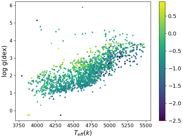
Figure 1: Distribution of barium stars adopted as positive samples in the plane of $T_{\mathrm{eff}}$-$\log g$, the colors indicate the [Fe/H] of stars. The triangle symbols indicate the barium star sample provided by L18, and the dot symbols indicate samples provided by N19.

In order to train and test the classifier, we collected known samples of barium stars and non-barium stars. The data set of barium stars used in this work has two parts. The first part consists of 867 s-process-rich stars. These stars were obtained by cross-matching LAMOST DR9 catalog with the catalog provided by N19, including 48 Ba-only, 642 Sr-only, and 177 both Sr- and Ba- enhancement candidates. The second part consists of 810 barium star spectra. After cross-matching LAMOST DR9 catalog with 719 barium stars provided by L18, we obtained 577 barium stars with 907 spectra. Then removing repeated spectra with signal-to-noise ratio (S/N) <30 pixel${}^{-}1$ in 907 spectra, we finally obtained 810 spectra.

In addition, the spectra of negative samples (non-barium stars) were randomly selected from LAMOST DR9 F, G, and K type giants catalog and based on the following selection criteria: S/N >30 pixel${}^{-}1$ (both on the g-band and r-band, which aim to be consistent with the screening of positive samples according to the rules of N19) and log $g$ <3.5 (Giants are defined by this criterion (Liu et al., 2014)). Figure 1 presents the stellar parameter space of our sample in the plane of $T_{\mathrm{eff}}$-$\log g$.

The spectra were preprocessed based on the following steps.

(1) Correct the wavelength by the radial velocity: the wavelengths were corrected by the following formula.

$$w_{new}(n)=w(n)/(1+z),$$ (1)

where $w(n)$ represents the wavelengths of an observed spectrum, and $z$ represents the redshift of this star. The $z$ was calculated by the LAMOST 1D pipeline (Luo & Zhao, 2001).

(2) Normalization: The flux of each spectrum is normalized to the range [0,1] according to the following formula.

$$\hat{x}=\frac{x-min(x)}{max(x)-min(x)},$$ (2)

where $x$ represents flux of an observed spectrum, and $min(x)$ and $max(x)$ represent the minimum and maximum flux of the spectrum $x$.

3 Method

3.1 LGBM Algorithm

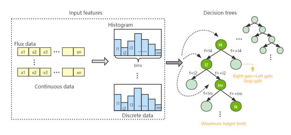
Figure 2: This is a process diagram of how LGBM constructs a decision tree for classification or prediction. The model discretizes the input features and establishes the histogram. Then according to these established histograms, features are selected as nodes to split and build a decision tree. Each decision tree would give a possible result, and the final result will be calculated according to the results of all the decision trees.

The Light Gradient Boosting Machine algorithm proposed by Microsoft in 2017 is a gradient boosting tree framework, which is an ensemble learning algorithm (Ke et al., 2017). Figure 2 shows the theoretical process of the construction of an LGBM model. An LGBM model consists of several decision trees. Each tree is a weak learner, which is built by splitting leaf nodes. LGBM uses the histogram method to split features and build leaf nodes. As features are input into the model, continuous data are discretized and histograms are built. Each unit of the histogram consists of statistically discrete data, which are called a bin. For each feature, the histogram stores two kinds of information: the sum of gradients for the samples in each bin ($H[i].g$), and the number of samples in each bin ($H[i].n$). The model traverses histograms instead of the whole data and splits features according to the bin with the maximum gain. The steps for calculating gain are as follows.

The first is calculating gradients. Suppose that $H$ denotes a storage structure in the histogram. For the ith bin in the histogram, the current gradient sum of the left node is

$$S_{L}=S_{L}+H[i].g;$$ (3)

H[i].g represents the gradient value of the corresponding feature of each bin. The number of samples on the left leaves is

$$n_{L}=n_{L}+H[i].n;$$ (4)

H[i].n represents the number of features corresponding to each bin. For the input current gradient sum of parent node $S_{P}$, the output current gradient sum of the right node is

$$S_{R}=S_{P}-S_{L};$$ (5)

Input the number of samples on parent leaves $n_{P}$ and calculate the number of samples on right leaves

$$n_{R}=n_{P}-n_{L};$$ (6)

Then, the output loss function is

$$\Delta loss=\frac{S^{2}_{L}}{n_{L}}+\frac{S^{2}_{R}}{n_{R}}-\frac{S^{2}_{P}}{n_{P}}.$$ (7)

The number of bins in the histogram is smaller than the size of the continuous feature, which can reduce memory consumption. In addition, the tree keeps growing until the maximum depth limit is reached, which can prevent overfitting.

Iteration method assures the minimum loss of the loss function when building a decision tree. The result of the model is a comprehensive consideration of all weak learners’ results: combining them into a strong learner. The results are held in the leaves which are at the ends of the branches. In the classifier, a result is a number that reflects the degree of being a barium star or not. In prediction, the result reflects the most probable value. When the depth of trees reaches the set maximum depth (max_depth), the process of building the LGBM model will stop. In the testing process, after inputting sample sets into the built model, every sample starts from the root node and goes through the branches down to the leaves, and then the results can be obtained.

The key parameters of the LGBM algorithm which we used are as follows.

• n_estimators, which define the number of decision trees (the number of iterations), which is the first parameter to be considered. Too small or too large will lead to underfitting or overfitting.

• max_depth, which defines the maximum depth of each decision tree. This parameter is inversely proportional to overfitting.

• num_leaves, which defines the number of leaves on each decision tree. It controls the complexity of the tree model. Ideally, num_leaves $\leq 2^{max\_depth}$.

For the LGBM models, we set the estimators from 100 to 1000 and the step size is 100. After training, we found that the model gradually fitted after about 300 for the Sr classifier, and 200 for Ba classifier. These fields then were narrowed down to 200 to 400 for Sr and 100 to 300 for Ba, both in steps of 50. After continually training and searching for fitting points, the fields were narrowed eventually to 300 to 310 for Sr and 215 to 225 for Ba, both in steps of 1. In this way, we can be sure that estimators should be set at 303 for Sr classifier and 220 for Ba classifier. The max depth (from 3 to 14 in steps of 1 initially) and leaves’ number (from 10 to 30 in steps of 1 initially) are set in a similar way. Besides, we add hyperparameters (the minimum weight of child nodes and the minimum number of samples, L1 and L2 regularization coefficient, etc.) to prevent over-fitting. The procedure of parameters searching is supported by GridSearchCV, which is a tool provided by scikit-learn (Abraham et al., 2014) and is used in both classification and prediction to set parameters.

3.2 SVM

SVM is a two-class classification model which is based on statistical learning theory. SVM was firstly introduced by (Vapnik, 1995) and then was widely employed to solve astronomical problems (Huertas-Company et al., 2008; Peng et al., 2012; Bu et al., 2014). Here is a brief introduction to the principle of the SVM algorithm.

We input the training data as $T={(x_{1},y_{1}),(x_{2},y_{2}),...,(x_{N},y_{N})}$, where $x_{i}\in R^{n},y_{i}\in\{-1,1\},i=1,2,...,N.$ , $x_{i}$ represents feature vectors and $y_{i}$ represents category markers. We suppose there is a hyperplane that separates positive examples from negative ones. The points x that lie on the hyperplane satisfy $\omega\cdot x+b=0$, where $\omega$ is normal to the hyperplane, and $|b|$ is the perpendicular distance from the hyperplane to the origin. Then SVM can be formulated as:

$$\left\{\begin{array}[]{lr}max\frac{1}{\|\omega\|}+C\sum_{i=1}^{N}\epsilon,&\\ subject\quad to\quad y_{i}(\omega^{T}x_{i}+b)\geq 1-\epsilon_{i},i=1,2,...,N,&\\ \epsilon_{i}\geq 0,i=1,2,...,M,\end{array}\right.$$ (8)

where $C$ is the penalty factor and $\epsilon_{i}$ are the slack variables. Then this problem can be transformed into the following formula

$$min_{\alpha}\frac{1}{2}\sum_{i=1}^{N}\sum_{j=1}^{N}\alpha_{i}\alpha_{j}y_{i}y_{j}(x_{i}\cdot x_{j})-\sum_{i=1}^{N}\alpha_{i},$$ (9)

which is subject to

$$\left\{\begin{array}[]{lr}\sum_{i=1}^{N}\alpha_{i}y_{i}=0,&\\ 0\leq\alpha_{i}\leq C,&i=1,2,...,N,\end{array}\right.$$ (10)

where $\alpha_{i}$ are the Lagrange multipliers $\alpha$ for each sample ($x_{i},y_{i}$). After using sequential minimal optimization (SMO) to find the unique variable $\alpha_{i}^{*}$, in the target function, we can obtain the optimal results. In this case, $\omega$ is

$$\omega^{*}=\sum_{i=1}^{N}\alpha_{i}^{*}y_{i}x_{i}.$$ (11)

When the features are nonlinear. SVM introduces the kernel function $K(x,z)$ to map the data set into high-dimensional space and classifies it in this space by a linear classifier. The equation (9) can be replaced by the following formula

$$min_{\alpha}\frac{1}{2}\sum_{i=1}^{N}\sum_{j=1}^{N}\alpha_{i}\alpha_{j}y_{i}y_{j}K(x_{i}\cdot x_{j})-\sum_{i=1}^{N}\alpha_{i}.$$ (12)

There are different types of kernel functions that can be selected. In our work, we used a radial basis function which is the most widely used and has good performance in both large and small samples: $K(x,z)=exp(-\frac{\|x-z\|^{2}}{2\sigma^{2}})$, where $z$ is the kernel function center and $\sigma$ is the width parameter of the function that controls the radial scope of the function. In this case, $\omega$ is

$$\omega^{*}=\sum_{i=1}^{N}\alpha_{i}^{*}y_{i}K(x_{i}\cdot x_{j}).$$ (13)

Then we just need to compute the sign of the following function

$$f(x)=sign(\omega\cdot x+b).$$ (14)

4 Experiment

There are mainly two research objectives for this experiment. First, train the classification model using the barium samples (L18 and N19) to separate the barium stars from the normal giant stars. This model will be used to search for new barium giant candidates from LAMOST DR9 in subsequent work. Second, building the element abundance prediction model using the barium samples with [Ba/Fe] and [Sr/Fe] labels(N19). This model will be used to estimate [Ba/Fe] and [Sr/Fe] of the newly found barium giant stars in the subsequent work. The following content of this chapter will introduce our experiment process in detail.

4.1 Performance Metric

The performance of a machine-learning classification model is usually evaluated by precision, recall, and F1-score (Forman, 2003), which are parameters calculated from the confusion matrix. These three evaluation criteria are defined as follows.

$$precision=\frac{TP}{TP+FP};$$ (15)

$$recall=\frac{TP}{TP+FN};$$ (16)

$$F1-score=\frac{2*(Precision*Recall)}{(Precision+Recall)}.$$ (17)

Since the test set consists of labeled samples, it is easy to judge if the classifier’s classification results are correct on the test set. TP is the number of true barium samples that are correctly classified as positive samples by the model. FP is the number of non-barium stars that are misclassified as positive samples by the model. Similarly, TN is the number of non-barium stars that are correctly classified as negative samples by the model, and FN is the number of true barium stars that are misclassified as negative stars by the model.

Precision is defined as the percentage of correct barium star predictions of all stars classified as positive, while the recall is the fraction of barium stars correctly classified as positive to the total number of barium samples. F1-score is the harmonic mean of the precision and recall.

In prediction, two methods are used to evaluate the performance of the model.

1.Mean absolute error (MAE). It can avoid compensating error and accurately reflect the actual prediction error, which is a commonly used performance metric of a regression model.

$$MAE=\frac{1}{n}\sum_{i=1}^{n}\\ y_{test}^{i}-Y_{test}^{i},$$ (18)

where $n$ is the number of samples in the testing data set, $y_{test}^{i}$ is the target value of samples and $Y_{test}^{i}$ is the result of the predictor corresponding to $y_{test}^{i}$. It can measure the actual error between the target value and the result of the predictor.

2.Standard deviation ($\sigma$).

$$\sigma=\sqrt{\frac{\sum_{i=1}^{n}(E^{i}-E^{i^{\prime}})^{2}}{n}},$$ (19)

where $E^{i}=y_{test}^{i}-Y_{test}^{i}$, and $E^{i^{\prime}2}$ is the average of $E^{i}$. It can measure the dispersion degree of the difference between the prediction result and the target value, and evaluate the stability of the LGBM model.

4.2 Input Feature Selection

The method to distinguish barium stars mainly depends on the spectral line features. For example, N19 identified the s-process-rich candidates by comparing the strengths of the most conspicuous Sr ii ( 4077 Å and 4215 Å) and Ba ii lines( 4554 Å and 4934 Å) in template with observed spectra. L18 distinguished their barium samples based on the strong lines of s-process elements, particularly Ba ii at 4554 Å and Sr ii at 4077 Å. Considering our small sample size, we should choose the same feature band mentioned above as the input feature instead of the whole spectrum which contains too much irrelevant information. Well-chosen input features can improve classification accuracy substantially, or equivalently, reduce the amount of training data needed to obtain the desired level of performance (Forman, 2002). However, an important fact has to be considered. Barium stars are usually enriched not only with Ba or Sr but also with other s-process elements, such as Y, Zr, La, Ce, Nd, etc (Smiljanic et al., 2007b; Kong et al., 2018b). Although quite a lot of spectral lines of these elements are weak and it is not easy to estimate the abundances of corresponding elements accurately in low-resolution spectra, these characteristics can still be used as an important reference for the barium star criterion. Therefore, this study adopts two feature input methods to compare the effect and efficiency.

The first is to select several spectral bands containing the absorption line adopted by N19 and L18 as the input feature. We have additionally adopted the Ba ii line at 6496 Å. This absorption line is prominent and often used as an important basis for the discrimination of barium stars. When selecting the feature bandwidth on each side of an absorption line, we compared two wavelength regions: 70 Å and 20 Å. These selected spectral bands are shown in Figure 3. The second is inputting the entire spectrum as an input feature, and feature selection depends entirely on machine learning algorithms. Using this method, the absorption line features of other s-process elements will be a useful supplement although useless interference information is also increased.

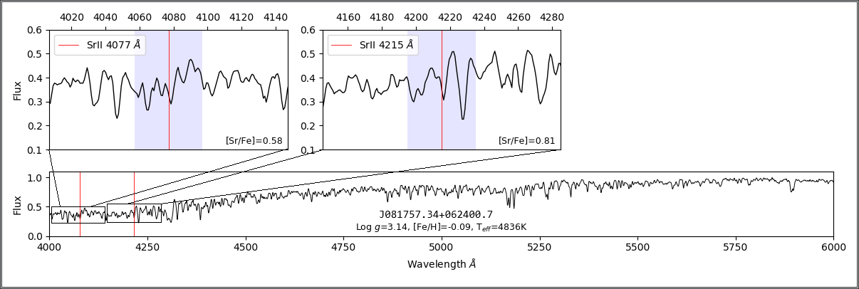
Sr enhanced

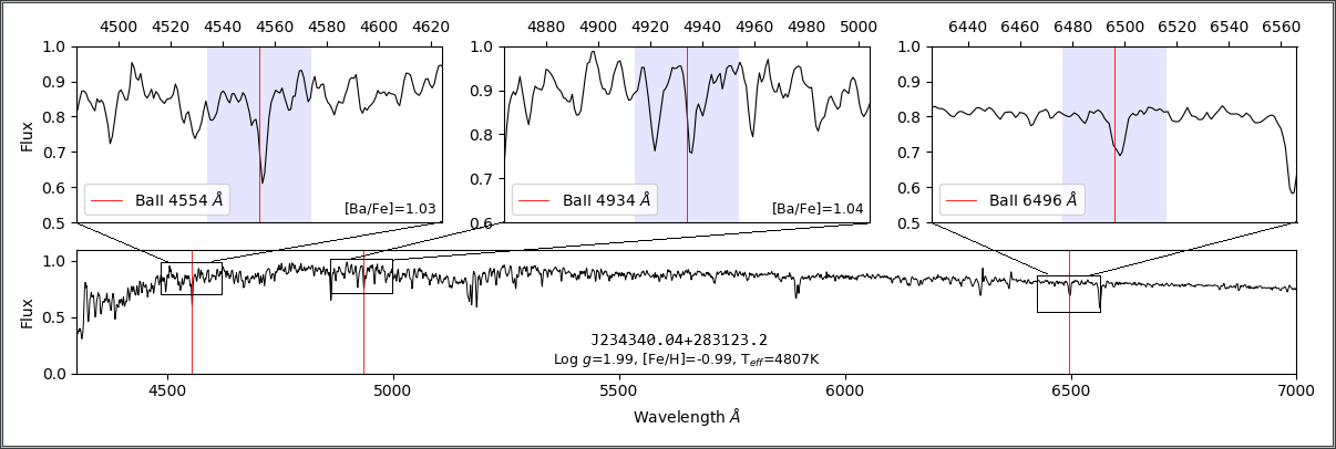
Ba enhanced

Figure 3: Local continuum spectra for Sr-only (J081757.34+062400.7) and Ba-only (J234340.04+283123.2) candidates randomly selected from the N19 dataset. The zoom-in ranges of wavelengths are feature bands of 70 Å, and the light blue part is feature bands of 20 Å.

4.3 Classification Construction

As mentioned in the introduction, N19 divided the s-process-rich candidates they found into three types: Sr-only, Ba-only, and both Sr- and Ba- enhancement candidates. Karinkuzhi et al. (2021) analyzed 15 of the brightest targets of the s-process-rich candidates searched by N19 based on high-resolution spectra, which consist of 13 Sr-only stars and two Ba-only stars. The analysis results show that four Sr-only stars present no s-process overabundances. They considered that the principal reason for the misclassification is that the Sr ii lines at 4077 and 4215 Å used by N19 are easily saturated and the 4215 Å line is strongly influenced by the strong CN bandhead at $\lambda$ 4216 Å. In fact, three of the four no-s stars considered as Sr-only by N19 are those being N-rich. Karinkuzhi et al. (2021) compared their derived Ba abundances with those determined by N19 based on the Ba ii lines at 4554 and 4934 Å and found that the agreement is much better for Ba than for Sr. Although our purpose is to search for s-process-rich candidates containing Sr-rich or Ba-rich stars, based on the reasons above and our preliminary experiment, instead of taking Sr-only and Ba-only as the same category, we have built two classifiers to identify Sr-rich and Ba-rich candidates respectively, which are called Sr-classifier and Ba-classifier.

We divided the positive sample into two parts. The first part consists of 1629 Sr-enhanced candidates, which includes 819 Sr-enhanced (642 Sr-only and 177 both Sr- and Ba-) barium stars from N19 and 810 barium stars from L18. The other part consists of 1035 Ba-enhanced candidates, which includes 225 Ba-enhanced (48 Ba-only and 177 both Sr- and Ba-) barium stars from N19 and 810 barium stars from L18. Two independent classifiers are constructed based on the two parts of the data set respectively.

Oh et al. (2020) used interpolation to augment the time-series data. This method interpolates the virtual new collection points into each collection point of the original time-series, which obtains the interpolated time-series. Then they generate a new time-series by extracting random data points. Data augmentation can be achieved based on this method and can keep the trend information of the original time-series. Considering the similar 2D data patterns, we used the same method on spectral data to improve the generalization capabilities of the machine learning model. The basic idea is to interpolate the information of flux at the wavelengths of every spectrum with the range of 4000-8098 Å, and then extract data points at regular intervals to generate new spectra. The number ratio of the training set and testing set is 8:2 by random division. We enhanced the training data set of Sr-enhanced up to 3893 and Ba-enhanced up to 2474 by this method, but the testing sets were not augmented. Table 3 lists the composition of the data set.

Table 1: The Comparison Results of LGBM and SVM with Different Input Features. Checkmarks mean the feature bands selected by the model and the corresponding feature width intercepted.

Classifiers		Sr enhanced			Ba enhanced
Feature width	70Å	✓			✓
	20Å		✓			✓
Feature bands	4077Å(Sr II)	✓	✓
	4215 Å(Sr II)	✓	✓
	4554 Å(Ba II)				✓	✓
	4934 Å(Ba II)				✓	✓
	6496 Å(Ba II)				✓	✓
Whole spectrum	4000-8000Å			✓			✓
LGBM	F1-score	94.60%	95.07%	96.92%	96.70%	96.71%	96.87%
	Recall	92.82%	93.54%	96.05%	96.84%	97.13%	97.70%
	Precision	96.46%	96.66%	97.81%	96.56%	96.30%	96.03%
SVM	F1-score	93.51%	91.93%	96.83%	96.47%	96.01%	96.02%
	Recall	89.23%	86.89%	95.29%	96.55%	96.84%	95.83%
	Precision	98.22%	97.58%	98.37%	96.39%	95.20%	96.21%

In this experiment, we employed the LGBM algorithm. Considering that SVM has excellent performance on small samples, we also adopted the SVM algorithm for comparison. The classification results of inputting different feature bands are compared and shown in Table 1. There is a point here. The absorption line profiles of an element are affected not only by the abundance value of the element but also by other factors, mainly atmospheric parameters. For the feature bands input method, atmospheric parameters ($T_{eff}$, Log $g$, [Fe/H]) have been normalized to [0,1] and added as the feature input because the model cannot determine them from several bands with the wavelength range of 20 Å or 70 Å.

It should be noted that the results in Table 1 are the average of three metrics of five-fold. In order to evaluate the reliability of our model, the five-fold cross-validation was used and the Sr-enhanced samples and Ba-enhanced samples were divided into five equal parts respectively. One of five parts of all data was taken as the test data, 10% of the remaining four parts was used as a validation set, and the rest was used as a training set. The process was repeated five times by moving the test data portion.

For the overall performance of the classification in Table 1, the LGBM algorithm performs excellently and stably in general. For the Sr classifier, the different selection of features has a greater impact on the Recall, especially for the SVM algorithm. For the Ba classifier, there is no significant difference between the classification results obtained by the two algorithms using different feature bands. In other words, using prior knowledge to select different input features does not improve the performance of the classifier, the reason may be that when we use the whole spectra (4000-8000 Å) as input feature, the other s-process elements we analyzed in 4.2 above, such as Y, Zr, La, Ce and Nd, provide additional judgment bases, which can overcome the interference caused by other absorption lines.

In this experiment, the best model (The feature selection is the whole spectra): Sr classifier consists of 303 decision trees (i.e., $n\_estimatiors=303$) and 14 leaves on each tree (i.e., $num\_leaves=14$) with heights of 12 (i.e., $max\_depth=12$) based on LGBM model. Ba classifier based on LGBM consists of 220 decision trees (i.e., $n\_estimatiors=220$) and 9 leaves on each tree (i.e., $num\_leaves=9$) with heights of 4 (i.e., $max\_dept=4$). The parameters based on SVM are as follows: the penalty parameter is 759 (i.e., $C=759$) and kernel coefficient is 0.005 (i.e., $gamma=0.005$) in Sr classifier, and the penalty parameter is 1370 (i.e., $C=1370$) and kernel coefficient is 0.0005 (i.e., $gamma=0.0005$) in Ba classifier. The feature selection is 20 Å band: Sr classifier consists of 523 decision trees (i.e., $n\_estimatiors=523$) and 13 leaves on each tree (i.e., $num\_leaves=13$) with heights of 5 (i.e., $max\_depth=5$) based on LGBM model. Ba classifier based on LGBM consists of 217 decision trees (i.e., $n\_estimatiors=217$) and 18 leaves on each tree (i.e., $num\_leaves=18$) with heights of 5 (i.e., $max\_depth=5$). The parameters based on SVM are as follows: the penalty parameter is 20 (i.e., $C=20$) and kernel coefficient is 15 (i.e., $gamma=15$) in Sr classifier, and the penalty parameter is 1848 (i.e., $C=1848$) and kernel coefficient is 0.5 (i.e., $gamma=0.5$) in Ba classifier. The feature selection is 70 Å band: Sr classifier consists of 665 decision trees (i.e., $n\_estimatiors=665$) and 13 leaves on each tree (i.e., $num\_leaves=13$) with heights of 4 (i.e., $max\_depth=4$) based on LGBM model. Ba classifier based on LGBM consists of 211 decision trees (i.e., $n\_estimatiors=211$) and 9 leaves on each tree (i.e., $num\_leaves=9$) with heights of 5 (i.e., $max\_depth=5$). The parameters based on SVM are as follows: the penalty parameter is 30 (i.e., $C=30$) and kernel coefficient is 1 (i.e., $gamma=1$) in Sr classifier, and the penalty parameter is 1378 (i.e., $C=1378$) and kernel coefficient is 0.01 (i.e., $gamma=0.01$) in Ba classifier.

Table 2: Abundance of Partial Barium Giants Reported by N19.

2MASS	[Sr/Fe]		[Ba/Fe]		Sr-only	Ba-only	Sr- and Ba-enhancement
	4077Å	4215Å	4554Å	4934Å
J231231.643+430416.61	0.98	0.98	$-0.04$	$-0.06$	✓	$\times$	$\times$
J005748.459+425733.24	0.92	0.87	0.39	$-0.14$	✓	$\times$	$\times$
J060926.438+283923.42	0.76	$-0.13$	$-0.01$	$-0.20$	✓	$\times$	$\times$
J231517.618+164636.08	$-0.16$	$-0.07$	1.04	1.12	$\times$	✓	$\times$
J032435.984+36086.22	0.62	$-0.04$	1.00	0.93	$\times$	✓	$\times$
J183447.556+354651.68	0.75	0.73	0.85	1.04	$\times$	✓	$\times$
J064614.085+162156.82	0.93	0.88	1.01	0.86	$\times$	$\times$	✓
J222439.264+083051.67	0.80	0.53	0.84	$-0.11$	$\times$	$\times$	✓
J024832.227+372351.13	0.83	$-0.05$	1.02	0.89	$\times$	$\times$	✓

Table 3: Number of Training and Testing Data Sets in the Classification.

Numbers		Sr classifier			Ba classifier
Spectra number of barium stars		1629	819 (N19)	642 Sr-only	1035	225 (N19)	48 Ba-only
				177 Sr&Ba			177 Sr&Ba
			810 (L18)			810 (L18)
Positive samples number	training set(before augmented)	1303			828
	training set(after augmented)	3893			2474
	testing set	326			207
Ratios of positive and negative samples		1:1			1:1

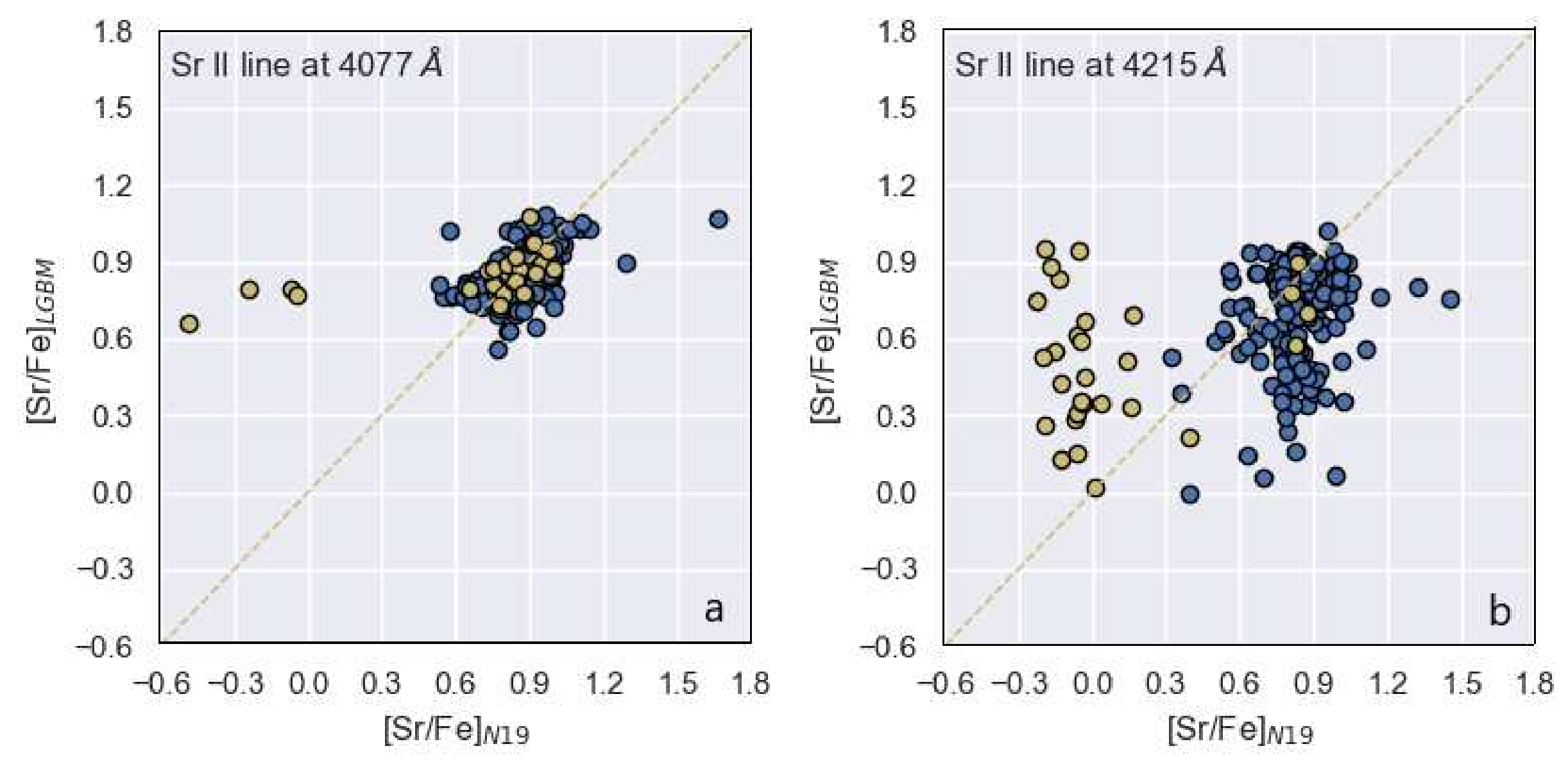
Figure 4: Comparisons of the Sr abundances calculated by our work ([Sr/Fe]_LGBM) and values determined from N19 ([Sr/Fe]_N19). The yellow line represents that the predicted value is equal to the target value. The yellow dot represents the point at which $\mid$[Sr/Fe$]_{4077\AA}$ - [Sr/Fe$]_{4215\AA}\mid\geq 0.5$ in N19. The left shows the differences between [Sr/Fe]_LGBM and [Sr/Fe]_N19 in the prediction of 4077 Å (Sr ii), and the right shows these differences in the prediction of 4215 Å (Sr ii).

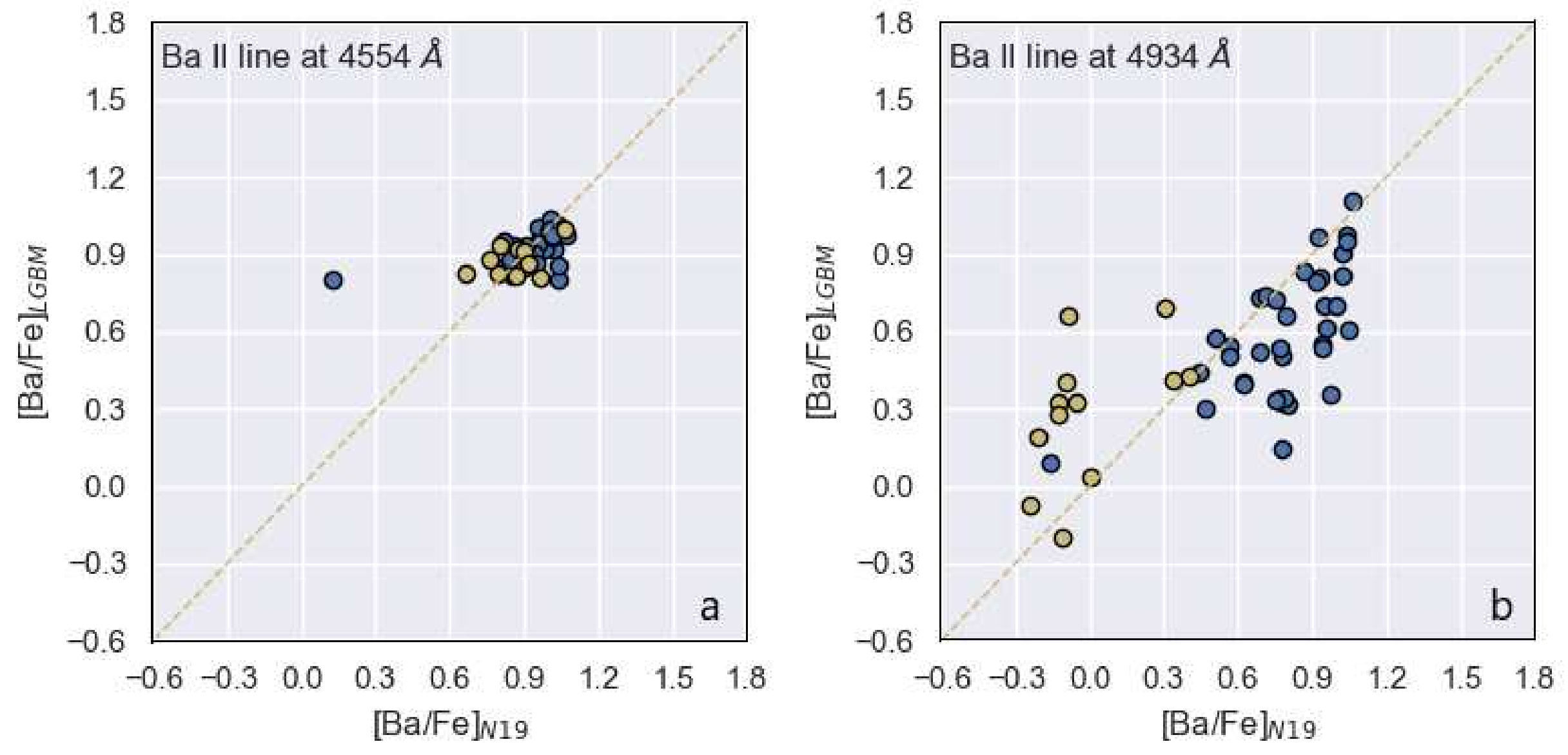
Figure 5: Comparisons of the Ba abundances calculated by our work ([Ba/Fe]_LGBM) and values determined from N19 ([Ba/Fe]_N19). The yellow line signifies that the predicted value is equal to the target value. The yellow dot represents the point at which $\mid$[Ba/Fe$]_{4554\AA}$ - [Ba/Fe$]_{4934\AA}\mid\geq 0.5$ in N19. The left shows the differences between [Ba/Fe]_LGBM and [Ba/Fe]_N19 in the prediction of 4554 Å (Ba ii), and the right shows these differences in the prediction of 4934 Å (Ba ii).

4.4 Prediction Construction

Since L18 did not provide [Ba/Fe] and [Sr/Fe] of barium stars, we only used N19 as the data set. Table 2 provides the [Ba/Fe] and [Sr/Fe] at different lines of several barium stars that come from N19.

In this work, we use the LGBM algorithm to predict the [Ba/Fe] and [Sr/Fe]. Sr enhanced predictor consists of 800 trees (i.e., n_estimatiors = 800) and 20 leaves on each tree (i.e., num_leaves = 20) with heights of 10 (i.e.,max_depth = 10). We also set other parameters (i.e., min_child_samples = 20, min_child_weight = 0.01). When continuously adjusting parameters through GridSearchCV, the parameters of the Ba-enhanced predictor were numerically the same as Sr enhanced predictor. Using [Ba/Fe] and [Sr/Fe] provided by N19 as labels, the selection of model feature bands and the performance of our models are shown in Table 4.

As seen from Table 4, the prediction result of [Sr/Fe] at the 4077 Å is less scattered, MAE = 0.09 and the standard deviation ($\sigma$) is about 0.16; while the prediction result of [Ba/Fe] at 4554 Å is closer to its label value than that at line 4934 Å, with MAE = 0.07 and $\sigma$ = 0.12.

Figure 4 and Figure 5 show the comparison between the abundance provided by N19 and the LGBM prediction results. From Figure 4(b), it can be seen that in the range of [Sr/Fe]_N19 $\textless$ 0.3, the prediction value of [Sr/Fe]_LGBM is much higher. The same situation also appears in [Ba/Fe]_4934Å. In this part of the data (most of the yellow dots), it can be seen from the lists provided by N19 that the difference in abundance obtained by different absorption lines of the same element is relatively large: $\mid$[Sr/Fe$]_{4077\AA}$ - [Sr/Fe$]_{4215\AA}\mid\geq 0.5$, $\mid$[Ba/Fe$]_{4554\AA}$ - [Ba/Fe$]_{4934\AA}\mid\geq 0.5$. Therefore, the high dispersion of prediction results in this part is probably due to the insufficient accuracy of the sample labels.

Table 4: The Results of LGBM in Predicting [Ba/Fe] and [Sr/Fe].

Predictors		[Sr/Fe]		[Ba/Fe]
		4077Å	4215Å	4554Å	4934Å
Feature bands	4057-4097Å(Sr ii)	✓
	4195-4235Å(Sr ii)		✓
	4534-4574Å(Ba ii)			✓
	4925-4965Å(Ba ii)				✓
Performance	MAE	0.09	0.20	0.07	0.26
	$\sigma$	0.16	0.29	0.12	0.32

The high-resolution abundance analysis of 15 barium star candidates of Karinkuzhi et al. (2021) showed that [Sr/Fe] obtained by N19 based on low-resolution spectra is generally higher, while [Ba/Fe] is generally lower. This means that searching for barium stars based on the model of the Ba classifier will get more reliable barium star candidates than the Sr classifier, while an accurate abundance value will depend on high-resolution spectral analysis.

4.5 Comparison with Other Methods

Table 5: The Comparison Results of SVM, KNN, RF and XGBoost based on the whole spectra.

Model	Sr enhanced			Ba enhanced
	F1-score	Recall	Precision	F1-score	Recall	Precision
KNN	92.58%	94.08%	91.13%	91.87%	95.69%	88.34%
RF	94.00%	92.82%	95.21%	94.68%	94.54%	94.81%
XGBoost	96.90%	96.18%	97.63%	96.29%	96.84%	95.74%
SVM	96.83%	95.29%	98.37%	96.02%	95.83%	96.21%
LGBM	96.92%	96.05%	97.81%	96.87%	97.70%	96.03%

In addition to LGBM and SVM, we also adopt three other popular algorithms (KNN, Random Forest (RF) and XGBoost) to compare the classifier performance in the whole feature bands, which often perform well in data science tasks. RF and XGBoost are similar to LGBM which is based on decision trees. For the Sr classification model, we set the decision tree number to 297 and the maximum depth to 12 in RF, while we set the decision tree number to 401, the maximum depth to 7 and the minimum weight of child nodes to 5 in XGBoost. For the Ba classification model, we set the decision tree number to 735 and the maximum depth to 13 in RF, while we set the decision tree number to 260, the maximum depth to 5 and the minimum weight of child nodes to 5 in XGBoost. KNN is a classical machine learning algorithm that classifies barium stars by measuring the distance between different features. We set 18 neighbors near each sample to find for measurement both in Sr classifier and Ba classifier. Through repeated training and testing, we finally arrived at the result of the comparison, which is shown in Table 5. We can see that the LGBM still performs best in general, and XGBoos has a very close excellent performance.

5 Conclusion

We constructed an Sr classifier, Ba classifier and abundance prediction models based on small samples of barium star candidates. SVM, KNN, RF, XGBoost and LGBM are applied for comparison in classifiers. The results show that the LGBM algorithm performs best on identifying barium stars, for Sr classification, Precision=97.81%, Recall=96.05%; for Ba classification, Precision= 96.03%, Recall=97.70%. The prediction results show that Sr predictor based on Sr ii at 4077 Å and Ba predictor based on Ba ii at 4554 Å performed better.

Besides the powerful learning ability of machine learning, the good classification results may also be related to our samples. The positive samples we adopted all have prominent Ba or Sr absorption lines, which is obviously different from normal giants. For the prediction model, the predicted [Ba/Fe] at 4544Å and [Sr/Fe] at 4077 Å are well consistent with the labels, which may also be because the distribution range of label values is narrow, and the predicted values of the model tend to fall into this range.

After the comparison from using different feature bands plus atmospheric parameters and inputting the entire spectrum for the training data, the results show that the precision and recall of the entire spectrum are the best. This indicates that machine learning algorithms are fully capable of learning useful features from complex data to optimize their model parameters, even if the number of training samples is not very large.

The results of the high-resolution spectral analysis show that [Sr/Fe] of the data set from N19 is higher and [Ba/Fe] of most data is lower. Therefore, the candidates obtained by Ba classifier will be more reliable when using the model to search for barium star candidates in the future.

This work is supported by the National Natural Science Foundation of China (NSFC) under Grant Nos. 11803016, U1931209 and 11873037. Software: LGBM(https://lightgbm.readthedocs.io/en/latest/pythonapi/lightgbm.LGBMClassifier.html), Scikit-learn: Machine Learning in Python (https://scikit-learn.org/stable/index.html).

References

- Abraham et al. (2014) Abraham, A., Pedregosa, F., Eickenberg, M., et al. 2014, FRONTIERS IN NEUROINFORMATICS, 14
- Allen & Barbuy (2006) Allen, D. M., & Barbuy, B. 2006, A&A, 454, 895, doi: 10.1051/0004-6361:20064912
- Bidelman (1981) Bidelman, W. P. 1981, AJ, 86, 553, doi: 10.1086/112913
- Bidelman & Keenan (1951) Bidelman, W. P., & Keenan, P. C. 1951, ApJ, 114, 473, doi: 10.1086/145488
- Boffin & Jorissen (1988) Boffin, H. M. J., & Jorissen, A. 1988, A&A, 205, 155
- Bu et al. (2014) Bu, Y., Chen, F., & Pan, J. 2014, New Astronomy, 28, 35, doi: https://doi.org/10.1016/j.newast.2013.09.007
- Cui et al. (2012) Cui, X.-Q., Zhao, Y.-H., Chu, Y.-Q., et al. 2012, Research in Astronomy and Astrophysics, 12, 1197, doi: 10.1088/1674-4527/12/9/003
- de Castro et al. (2016) de Castro, D. B., Pereira, C. B., Roig, F., et al. 2016, MNRAS, 459, 4299, doi: 10.1093/mnras/stw815
- Forman (2002) Forman, G. 2002, in Principles of Data Mining and Knowledge Discovery, ed. T. Elomaa, H. Mannila, & H. Toivonen (Berlin, Heidelberg: Springer Berlin Heidelberg), 150–162
- Forman (2003) Forman, G. 2003, J. Mach. Learn. Res., 3, 1289, doi: 10.1162/153244303322753670
- Gray & Griffin (2007) Gray, R. O., & Griffin, R. E. M. 2007, AJ, 134, 96, doi: 10.1086/518476
- Gray et al. (2011) Gray, R. O., McGahee, C. E., Griffin, R. E. M., & Corbally, C. J. 2011, AJ, 141, 160, doi: 10.1088/0004-6256/141/5/160
- Han et al. (1995) Han, Z., Eggleton, P. P., Podsiadlowski, P., & Tout, C. A. 1995, MNRAS, 277, 1443, doi: 10.1093/mnras/277.4.1443
- Huertas-Company et al. (2008) Huertas-Company, M., Rouan, D., Tasca, L., Soucail, G., & Le Fèvre, O. 2008, A&A, 478, 971, doi: 10.1051/0004-6361:20078625
- Jorissen et al. (1998) Jorissen, A., Van Eck, S., Mayor, M., & Udry, S. 1998, A&A, 332, 877. https://arxiv.org/abs/astro-ph/9801272
- Karinkuzhi et al. (2018) Karinkuzhi, D., Goswami, A., Sridhar, N., Masseron, T., & Purandardas, M. 2018, MNRAS, 476, 3086, doi: 10.1093/mnras/sty320
- Karinkuzhi et al. (2021) Karinkuzhi, D., Van Eck, S., Jorissen, A., et al. 2021, A&A, 654, A140, doi: 10.1051/0004-6361/202141629
- Ke et al. (2017) Ke, G., Meng, Q., Finely, T., et al. 2017, in Advances in Neural Information Processing Systems 30 (NIP 2017)
- Kong et al. (2018a) Kong, X. M., Bharat Kumar, Y., Zhao, G., et al. 2018a, MNRAS, 474, 2129, doi: 10.1093/mnras/stx2809
- Kong et al. (2018b) —. 2018b, MNRAS, 474, 2129, doi: 10.1093/mnras/stx2809
- Li et al. (2018) Li, Y.-B., Luo, A. L., Du, C.-D., et al. 2018, ApJS, 234, 31, doi: 10.3847/1538-4365/aaa415
- Liang et al. (2003) Liang, Y. C., Zhao, G., Chen, Y. Q., Qiu, H. M., & Zhang, B. 2003, A&A, 397, 257, doi: 10.1051/0004-6361:22021460
- Liu et al. (2014) Liu, C., Deng, L.-C., Carlin, J. L., et al. 2014, ApJ, 790, 110, doi: 10.1088/0004-637X/790/2/110
- Lu (1991) Lu, P. K. 1991, AJ, 101, 2229, doi: 10.1086/115845
- Luo & Zhao (2001) Luo, A. L., & Zhao, Y.-H. 2001, Chinese J. Astron. Astrophys., 1, 563, doi: 10.1088/1009-9271/1/6/563
- MacConnell et al. (1972) MacConnell, D. J., Frye, R. L., & Upgren, A. R. 1972, AJ, 77, 384, doi: 10.1086/111298
- McClure (1983) McClure, R. D. 1983, ApJ, 268, 264, doi: 10.1086/160951
- Merle et al. (2016) Merle, T., Jorissen, A., Van Eck, S., Masseron, T., & Van Winckel, H. 2016, A&A, 586, A151, doi: 10.1051/0004-6361/201526944
- Ness et al. (2015) Ness, M., Hogg, D. W., Rix, H. W., Ho, A. Y. Q., & Zasowski, G. 2015, ApJ, 808, 16, doi: 10.1088/0004-637X/808/1/16
- Norfolk et al. (2019) Norfolk, B. J., Casey, A. R., Karakas, A. I., et al. 2019, MNRAS, 490, 2219, doi: 10.1093/mnras/stz2630
- Oh et al. (2020) Oh, C., Han, S., & Jeong, J. 2020, Procedia Computer Science, 175, 64
- Peng et al. (2012) Peng, N., Zhang, Y., Zhao, Y., & Wu, X.-b. 2012, Monthly Notices of the Royal Astronomical Society, 425, 2599, doi: 10.1111/j.1365-2966.2012.21191.x
- Pereira (2005) Pereira, C. B. 2005, AJ, 129, 2469, doi: 10.1086/428755
- Pereira et al. (2011) Pereira, C. B., Sales Silva, J. V., Chavero, C., Roig, F., & Jilinski, E. 2011, A&A, 533, A51, doi: 10.1051/0004-6361/201117070
- Pompéia & Allen (2008) Pompéia, L., & Allen, D. M. 2008, A&A, 488, 723, doi: 10.1051/0004-6361:200809707
- Porto de Mello & da Silva (1997) Porto de Mello, G. F., & da Silva, L. 1997, ApJ, 476, L89, doi: 10.1086/310504
- Smiljanic et al. (2007a) Smiljanic, R., Porto de Mello, G. F., & da Silva, L. 2007a, A&A, 468, 679, doi: 10.1051/0004-6361:20065867
- Smiljanic et al. (2007b) —. 2007b, A&A, 468, 679, doi: 10.1051/0004-6361:20065867
- Smith (1984) Smith, V. V. 1984, A&A, 132, 326
- Smith & Lambert (1987) Smith, V. V., & Lambert, D. L. 1987, MNRAS, 226, 563, doi: 10.1093/mnras/226.3.563
- Sneden et al. (1981) Sneden, C., Lambert, D. L., & Pilachowski, C. A. 1981, ApJ, 247, 1052, doi: 10.1086/159114
- Tomkin & Lambert (1979) Tomkin, J., & Lambert, D. L. 1979, ApJ, 227, 209, doi: 10.1086/156720
- Vapnik (1995) Vapnik, V. N. 1995, The Nature of Statistical Learning Theory (The nature of statistical learning theory)
- Yang et al. (2016) Yang, G.-C., Liang, Y.-C., Spite, M., et al. 2016, Research in Astronomy and Astrophysics, 16, 19, doi: 10.1088/1674-4527/16/1/019