Regularized Barzilai-Borwein method

Abstract

We develop a novel stepsize based on Barzilai-Borwein method for solving some challenging optimization problems efficiently, named regularized Barzilai-Borwein (RBB) stepsize. We indicate that RBB stepsize is the close solution to a $\ell_{2}^{2}$-regularized least squares problem. When the regularized item vanishes, the RBB stepsize reduces to the original Barzilai-Borwein stepsize. RBB stepsize includes a class of valid stepsizes, such as another version of Barzilai-Borwein stepsize. The global convergence of the corresponding RBB algorithm is proved in solving convex quadratic optimization problems. One scheme for adaptively generating regularization parameters was proposed, named adaptive two-step parameter. An enhanced RBB stepsize is used for solving quadratic and general optimization problems more efficiently. RBB stepsize could overcome the instability of BB stepsize in many ill-conditioned optimization problems. Moreover, RBB stepsize is more robust than BB stepsize in numerical experiments. Numerical examples show the advantage of using the proposed stepsize to solve some challenging optimization problems vividly.

Keywords. stepsize, Barzilai-Borwein method, regularization, convergence, least squares

1 Introduction

In this paper, we consider the Barzilai and Borwein gradient method (BB method) [7] for the large scale unconstrained optimization problem

$$\min_{x\in\mathbb{R}^{n}}f(x),$$ (1.1)

where $f:\mathbb{R}^{n}\longrightarrow\mathbb{R}$ is a sufficiently smooth function. Its minimizer is denoted by $x_{*}$. The method is defined by

$$x_{k+1}=x_{k}+\frac{1}{\alpha_{k}}(-g_{k}),$$ (1.2)

where $x_{k}$ is the $k$th approximation to the optimal solution $x_{*}$ of (1.1), $g_{k}:=\nabla f(x_{k})$ is the gradient of $f$ at $x_{k}$. The scalar ${\alpha_{k}}$ is given by

$$\alpha_{k}^{BB1}\triangleq\alpha_{k}=\frac{s_{k-1}^{\text{T}}y_{k-1}}{s_{k-1}^{\text{T}}s_{k-1}},$$ (1.3)

where $s_{k-1}=x_{k}-x_{k-1}$ and $y_{k-1}=g_{k}-g_{k-1}$, $\frac{1}{\alpha_{k}}$ is called stepsize.

It is well known that the steepest descent (SD) method is the simplest gradient method in unconstrained optimization problems [40, 45]. In this method, locally, $-g_{k}$ is the search direction in which the objective function value decreases fastest, and the stepsize $\frac{1}{\alpha_{k}^{SD}}$ is determined by exact line search

$$\frac{1}{\alpha_{k}^{SD}}=\arg\min_{\alpha>0}f(x_{k}+\frac{1}{\alpha}(-g_{k})).$$ (1.4)

However, in practice, the steepest descent method is not very efficient and usually converges slowly. The main reason for the slow convergence speed of the steepest descent method is not the search direction, but the choice of stepsize. Accordingly, some practical inexactly line search strategies have been proposed successively [27, 5, 49, 39].

The BB method was first introduced by Barzilai and Borwein in 1988 [7]. As is known to all, the BB method requires few storage locations and affordable computation operations. In the BB method, assuming $s_{k-1}^{\text{T}}y_{k-1}>0$, the scalar $\alpha_{k}^{BB1}$ in (1.3) is the solution to the following least squares problem

$$\min_{\alpha\in\mathbb{R}}\|\alpha Is_{k-1}-y_{k-1}\|_{2}^{2}.$$ (1.5)

Here, another version of the BB scalar is to solve the least squares problem

$$\min_{\alpha\in\mathbb{R}}\|s_{k-1}-\frac{1}{\alpha}Iy_{k-1}\|_{2}^{2},$$

the minimizer of which is

$$\alpha_{k}^{BB2}=\frac{y_{k-1}^{\text{T}}y_{k-1}}{s_{k-1}^{\text{T}}y_{k-1}}.$$ (1.6)

By the Cauchy-Schwarz inequality [29], we know that $\alpha_{k}^{BB1}\leq\alpha_{k}^{BB2}$. For convenience, we focus on the $\alpha_{k}^{BB1}$ case in the next few sections, but for the $\alpha_{k}^{BB2}$ case, we will also perform a necessary analysis. From above, we know that the BB method approximates Hessian $\nabla^{2}f(x_{k})$ by the diagonal matrix $\alpha_{k}I$ at the $k$th iteration. Essentially, the BB method incorporates quasi-Newton approach to gradient method by the choice of stepsize. Thus, the BB method obtains a faster convergence speed than that of the steepest descent method. As a result, the BB method has received more and more attention from researchers because of its simplicity and the fact that it does not require storage of matrices to obtain convergence approximating the quasi-Newton method.

In the seminal paper [7], authors applied the BB method to solve the strictly convex quadratic problem

$$\min_{x\in\mathbb{R}^{n}}f(x)=\frac{1}{2}x^{\text{T}}Ax-b^{\text{T}}x,$$ (1.7)

where matrix $A\in\mathbb{R}^{n\times n}$ is a real symmetric positive definite matrix and $b\in\mathbb{R}^{n}$ is a given vector. In this case, the formula (1.3) can be written as

$$\alpha_{k}^{BB1}=\frac{s_{k-1}^{\text{T}}y_{k-1}}{s_{k-1}^{\text{T}}s_{k-1}}=\frac{s_{k-1}^{\text{T}}As_{k-1}}{s_{k-1}^{\text{T}}s_{k-1}}=\frac{g_{k-1}^{\text{T}}Ag_{k-1}}{g_{k-1}^{\text{T}}g_{k-1}}=\alpha_{k-1}^{SD}.$$ (1.8)

Similarly, we have

$$\alpha_{k}^{BB2}=\frac{y_{k-1}^{\text{T}}y_{k-1}}{s_{k-1}^{\text{T}}y_{k-1}}=\frac{s_{k-1}^{\text{T}}A^{2}s_{k-1}}{s_{k-1}^{\text{T}}As_{k-1}}=\frac{g_{k-1}^{\text{T}}A^{2}g_{k-1}}{g_{k-1}^{\text{T}}Ag_{k-1}}=\alpha_{k-1}^{MG},$$ (1.9)

where $\alpha_{k-1}^{MG}=\frac{g_{k-1}^{\text{T}}A^{2}g_{k-1}}{g_{k-1}^{\text{T}}Ag_{k-1}}$ is a straightforward line search is to minimize the gradient (MG) norm $\|g(x)\|_{2}$ along the direction $-g_{k-1}$ [18].

The BB method converges to the solution of (1.7) [41], even if there is no descent in the function value at every iteration. Especially when $n=2$, it converges $R$-superlinearly to the global minimizer [7]. Applying the BB method to problem (1.7), Dai and Liao proved that the BB method is R-linearly convergent [16] for any-dimensional strongly convex quadratic problems. In the past decades, this method has attracted the interest of many researchers. Consequently, the BB method has been extended to general constrained optimization, convex constrained optimization, nonlinear systems, optimal control, see [4, 21, 12, 38, 11, 14, 17, 36, 47] and the references therein.

Despite global convergence results of the BB method, one has to face the “backtracking phenomenon” of iterative residuals in numerical experiments [4, 10, 24]. As a matter of fact, this mysterious numerical phenomenon does not destroy the total downward tendency of iterative residual. As Powell’s last question [50] stated: the BB method is not monotone for $\{f(x_{k})\}$ and $\{\|g(x_{k})\|_{2}\}$, for what merit function is it monotone? Despite the excellent performance of the BB method and its variants in optimization community, the unstable performance due to its non-monotonicity may lead to poor results in some ill-conditioned problems.

In order to solve the problems mentioned above that arise in the BB method, we consider improving the least squares model (1.5) so as to obtain better quasi-Newton properties. More significantly, we are trying to answer Powell’s last question by a well known technique–regularization. It is well known that regularization approach has been widely investigated in such approximation problems [2, 3, 28, 34, 35, 48], which essentially employ the idea of penalty approach. Inspired by these effective methods, assuming $\Phi_{1}$ and $\Phi_{2}$ are two symmetric positive definite matrices such that $\Phi_{1}=\beta\Phi_{2}$, $\beta>0$, we consider the following regularized least squares problem

$$\min_{\alpha>0}\Big{\{}\|\alpha Is_{k-1}-y_{k-1}\|_{2}^{2}+\tau_{k}\|\alpha\Phi_{1}s_{k-1}-\Phi_{2}y_{k-1}\|_{2}^{2}\Big{\}},$$ (1.10)

where $\tau_{k}\geq 0$ is regularization parameter, $\|x\|_{2}^{2}=\langle x,x\rangle=x^{\text{T}}x$ is their inner product. In the next section, we will show that the solution to above least squares problem as follows

$$\alpha_{k}^{RBB}=\frac{s_{k-1}^{\mathrm{T}}y_{k-1}+\tau_{k}s_{k-1}^{\mathrm{T}}\Phi_{1}^{\text{T}}\Phi_{2}y_{k-1}}{s_{k-1}^{\mathrm{T}}s_{k-1}+\tau_{k}s_{k-1}^{\mathrm{T}}\Phi_{1}^{\text{T}}\Phi_{1}s_{k-1}}.$$ (1.11)

If $\tau_{k}=0$, (1.11) degenerates to the original Barzilai-Borwein scalar.

In sequal, we propose regularized Barzilai-Borwein (RBB) method for solving problem (1.7). In Section 3, we present global convergence properties, R-linear convergence rate of the RBB method (see Theorem 3.1, Theorem 3.2). In Section 4, we propose one scheme for generating regularization parameters. In Section 5, we consider an enhanced RBB method for general optimization problem (1.1), which has the advantages of low computing cost and fast convergence speed compared with the original RBB method. In Section 6, we present numerical results of the enhanced RBB method for some ill-conditioned quadratic and challenging spherical $t$-designs. We also demonstrate its numerical robustness. Finally, some conclusions are included in the last section of the paper.

2 Regularized BB method for solving problem (1.7)

In this section, for the problem (1.7), we will discuss some properties of RBB stepsize and the relation between it and other stepsizes. Let $\tau_{k}\geq 0$. Then the scalar $\alpha_{k}^{RBB}$ defined by (1.11) is the unique solution to (1.10). Proof.  Because problem (1.10) is a convex unconstrained optimization problem, the stationary point of the objective is none other than the unique solution to (1.10). Taking the first derivative of the objective in problem (1.10) with respect to $\alpha$ leads to the first-order optimality condition

$$\alpha(s_{k-1}^{\mathrm{T}}s_{k-1}+\tau_{k}s_{k-1}^{\mathrm{T}}\Phi_{1}^{\text{T}}\Phi_{1}s_{k-1})=s_{k-1}^{\mathrm{T}}y_{k-1}+\tau_{k}s_{k-1}^{\mathrm{T}}\Phi_{1}^{\text{T}}\Phi_{2}y_{k-1}.$$ (2.1)

With the first-order optimality condition (2.1), we have

$$\alpha=\frac{s_{k-1}^{\mathrm{T}}y_{k-1}+\tau_{k}s_{k-1}^{\mathrm{T}}\Phi_{1}^{\text{T}}\Phi_{2}y_{k-1}}{s_{k-1}^{\mathrm{T}}s_{k-1}+\tau_{k}s_{k-1}^{\mathrm{T}}\Phi_{1}^{\text{T}}\Phi_{1}s_{k-1}}.$$ (2.2)

Since $\Phi_{1}$ is symmetric positive definite matrix, the denominator of $\alpha$ in (2.2) is not equal to zero when $s_{k-1}\neq 0$. As a result, the $\alpha$ in (2.2) is the $\alpha_{k}^{RBB}$ in (1.11), this completes the proof. $\square$

Remark 2.1

Under the conditions of Theorem 2. If $\Phi_{1}=\Phi_{2}$, then the $\alpha_{k}^{RBB}$ in (1.11) with different regularization parameter $\tau_{k}$ possesses quasi-Newton properties.

For the quadratic optimization problem (1.7), we take $\Phi_{1}=\Phi_{2}=A$ in formula (1.11), which implies

$$\alpha_{k}^{RBB}=\frac{s_{k-1}^{\text{T}}(I+\tau_{k}A^{2})y_{k-1}}{s_{k-1}^{\text{T}}(I+\tau_{k}A^{2})s_{k-1}}.$$ (2.3)

Let

$$z_{\tau_{k}}=A_{\tau_{k}}s_{k-1},$$

where $A_{\tau_{k}}=(I+\tau_{k}A^{2})^{\frac{1}{2}}$. For the $\alpha_{k}^{RBB}$ in (2.3), we have

$$\alpha_{k}^{RBB}=\frac{z_{\tau_{k}}^{\mathrm{T}}Az_{\tau_{k}}}{z_{\tau_{k}}^{\mathrm{T}}z_{\tau_{k}}}.$$ (2.4)

By a well-know property of the Rayleigh quotient [29], we have

$$0<\lambda_{1}\leq\alpha_{k}^{RBB}\leq\lambda_{n},$$ (2.5)

where $\lambda_{1}$ and $\lambda_{n}$ denote the smallest and largest eigenvalues of $A$, respectively. This indicates that $\alpha_{k}^{RBB}$ lies in the spectrum of $A$.

From the Cauchy-Schwarz inequality, we have a rather simple but interesting result as follows

$$\frac{s_{k-1}^{\mathrm{T}}y_{k-1}}{s_{k-1}^{\mathrm{T}}s_{k-1}}\leq\frac{s_{k-1}^{\mathrm{T}}Ay_{k-1}}{s_{k-1}^{\mathrm{T}}As_{k-1}}\leq\frac{s_{k-1}^{\mathrm{T}}A^{2}y_{k-1}}{s_{k-1}^{\mathrm{T}}A^{2}s_{k-1}}.$$ (2.6)

Proposition 2.1

Assume that $s_{k-1}^{\mathrm{T}}y_{k-1}>0$ and $\tau_{k}\geq 0$. Then the $\alpha_{k}^{RBB}$ lies in $[\alpha_{k}^{BB1},\,\lambda_{n}]$ and is monotone with respect to parameter $\tau_{k}$.

Proof.  Let $h_{\tau_{k}}(\alpha)$ be the derivative of the $\alpha_{k}^{RBB}$ in (2.3) with respect to $\tau_{k}$. Then we have

$$h_{\tau_{k}}(\alpha)=\frac{s_{k-1}^{\mathrm{T}}A^{2}y_{k-1}s_{k-1}^{\mathrm{T}}s_{k-1}-s_{k-1}^{\mathrm{T}}y_{k-1}s_{k-1}^{\mathrm{T}}A^{2}s_{k-1}}{(s_{k-1}^{\mathrm{T}}(I+\tau_{k}A^{2})s_{k-1})^{2}}.$$

According to (2.6), we have $s_{k-1}^{\mathrm{T}}A^{2}y_{k-1}s_{k-1}^{\mathrm{T}}s_{k-1}-s_{k-1}^{\mathrm{T}}y_{k-1}s_{k-1}^{\mathrm{T}}A^{2}s_{k-1}\geq 0$. And since $s_{k-1}^{\text{T}}y_{k-1}>0$, we have $s_{k-1}^{\text{T}}(I+\tau_{k}A^{2})s_{k-1}\neq 0$. Thus $h_{\tau_{k}}(\alpha)\geq 0$. This shows that $\alpha_{k}^{RBB}$ increases monotonically with respect to $\tau_{k}$. In the case of $\tau_{k}=0$, we have $\alpha_{k}^{RBB}=\alpha_{k}^{BB1}$. And by the result of (2.5), we have $\alpha_{k}^{RBB}\in[\alpha_{k}^{BB1},\,\lambda_{n}]$. The proof is completed. $\square$

Lemma 2.1

Setting $\Phi_{1}=\Phi_{2}=A$. The solution to the second term in (1.10) is $\beta_{k}=\frac{s_{k-1}^{\mathrm{T}}A^{2}y_{k-1}}{s_{k-1}^{\mathrm{T}}A^{2}s_{k-1}}$. Inequalities (2.6) is equivalent to correspond exactly to the following relation

$$\alpha_{k}^{BB1}\leq\alpha_{k}^{BB2}\leq\beta_{k}.$$ (2.7)

Remark 2.2

Consequently, the regularization term in (1.10) is equivalent to a constraint imposed on the original least squares problem (1.5) to generate suitable small stepsize, improving the stability of BB method. At the same time, regularization parameter $\tau_{k}$ is adjusted to maintain the fast convergence of RBB method.

Dai et al. [15] proposed a family spectral gradient stepsizes by the convex combination of $\alpha_{k}^{BB1}$ and $\alpha_{k}^{BB2}$ as follows

$$\alpha_{k}^{Dai}=\gamma_{k}\alpha_{k}^{BB1}+(1-\gamma_{k})\alpha_{k}^{BB2},$$ (2.8)

where $\gamma_{k}\in[0,\,1]$. Similar to BB1 and BB2 stepsizes, each stepsize in this family also possesses quasi-Newton property. Here, the range of $\alpha_{k}^{RBB}$ is much broader compared to that of $\alpha_{k}^{Dai}$. The following theorem clearly expresses the generality of $\alpha_{k}^{RBB}$. We apply the RBB method to construct Algorithm 1 for finding the optimal solution to problem (1.7) in a stable manner. Under the conditions of optimization problem (1.7). The each $\alpha_{k}^{Dai}$ in (2.8) can be regard as a special case of the $\alpha_{k}^{RBB}$ in (2.3) as follows

1. $\alpha_{k}^{BB1}$ is a special case of the $\alpha_{k}^{RBB}$ when $\tau_{k}=0\,;$

2. $\alpha_{k}^{BB2}$ is a special case of the $\alpha_{k}^{RBB}$ when

   $$\tau_{k}=\frac{\alpha_{k}^{BB1}-\alpha_{k}^{BB2}}{(\frac{\|y_{k-1}\|_{2}}{\|s_{k-1}\|_{2}})^{2}(\alpha_{k}^{BB2}-\frac{y_{k-1}^{\mathrm{T}}Ay_{k-1}}{y_{k-1}^{\mathrm{T}}y_{k-1}})}\,;$$

3. $\alpha_{k}^{Dai}$ with $\gamma_{k}$ is a special case of the $\alpha_{k}^{RBB}$ when

   $$\tau_{k}=\frac{(1-\gamma_{k})(\alpha_{k}^{BB1}-\alpha_{k}^{BB2})}{(\frac{\|y_{k-1}\|_{2}}{\|s_{k-1}\|_{2}})^{2}(\gamma_{k}\alpha_{k}^{BB1}+(1-\gamma_{k})\alpha_{k}^{BB2}-\frac{y_{k-1}^{\mathrm{T}}Ay_{k-1}}{y_{k-1}^{\mathrm{T}}y_{k-1}})}\,,$$

   where $0\leq\gamma_{k}\leq 1$.

Input: Stopping criterion: $\varepsilon>0$, ${\text{MaxIt}>0}$;

Initialization: $A$, $b$, $k=1$, $x_{1}$, Regularization parameter: $\tau_{1}=0$; initial stepsize $t_{1}$;

1 while $k<{\rm{MaxIt}}$ and $\min\left\{\|x_{k+1}-x_{k}\|_{2},\,\frac{\|g_{k}\|_{2}}{\|g_{0}\|_{2}}\right\}>\varepsilon$ do

2      $g_{k}=Ax_{k}-b$.

3       $x_{k+1}=x_{k}-t_{k}g_{k}$.

4       $g_{k+1}=Ax_{k+1}-b$.

5       $s=x_{k+1}-x_{k}$, $y=g_{k+1}-g_{k}$.

6       $t_{k+1}=\frac{s^{\text{T}}s+\tau_{k}y^{\text{T}}y}{s^{\text{T}}y+\tau_{k}y^{\text{T}}Ay}$, for some $\tau_{k}\geq 0$.

7       $k=k+1$.

8 end while

Algorithm 1 RBB: Regularized Barzilai-Borwein algorithm for solving (1.7)

3 Convergence analysis about RBB method

In this section, global convergence and local R-linear convergence rate of Algorithm 1 will be proved. We state that the convergence analysis in this section is based on [33, 41]. Throughout this paper, denote the Euclidean condition number of matrix $A$ by

$$\kappa(A):=\|A\|_{2}\|A^{-1}\|_{2}=\frac{\lambda_{n}}{\lambda_{1}},$$

where $\lambda_{1}$ and $\lambda_{n}$ are the smallest and largest eigenvalues of $A$, respectively.

3.1 Global convergence property

To facilitate the analysis, we first introduce the following theorem. For the quadratic optimization problem (1.7). Let $\{x_{k}\}$ be the sequence of iterates generated by RBB method from a given vector $x_{0}$. Let $x_{*}$ be the unique optimal solution of (1.7). Denote residual $e_{k}=x_{*}-x_{k}$. Then for all positive integer $k$, we have

1. A$e_{k}=\alpha_{k}^{RBB}s_{k}$,

2. $e_{k+1}=\frac{1}{\alpha_{k}^{RBB}}(\alpha_{k}^{RBB}I-A)e_{k}$,

3. $s_{k+1}=\frac{1}{\alpha_{k+1}^{RBB}}(\alpha_{k}^{RBB}I-A)s_{k}$.

Proof.  Under the conditions in the theorem, we have $Ax_{*}-b=0$. It follows from $s_{k-1}=x_{k}-x_{k-1}$ and $x_{k+1}=x_{k}-\frac{1}{\alpha_{k}^{RBB}}g_{k}$ that $Ae_{k}=A(x_{*}-x_{k})=(Ax_{*}-b)-(Ax_{k}-b)=-g_{k}=\alpha_{k}^{RBB}s_{k}$ holds. It follows from $s_{k}=e_{k}-e_{k+1}$ and $Ae_{k}=\alpha_{k}^{RBB}s_{k}$, there holds $e_{k+1}=\frac{1}{\alpha_{k}^{RBB}}(\alpha_{k}^{RBB}I-A)e_{k}$. From $s_{k+1}=-\frac{1}{\alpha_{k+1}^{RBB}}g_{k+1}$, $s_{k}=-\frac{1}{\alpha_{k}^{RBB}}g_{k}$ and $g_{k+1}=(I-\frac{1}{\alpha_{k}^{RBB}}A)g_{k}$, the last equality follows directly. $\square$

For any residual vector $e_{k}$ with $k\geq 0$, there are constants $e^{k}_{1},\,e^{k}_{2},\,\dots,\,e^{k}_{n}$ such that

$$e_{k}=\sum_{i=1}^{n}e^{k}_{i}v_{i},$$ (3.1)

where $v_{1},\,v_{2},\,\ldots,\,v_{n}$ are the orthonormal eigenvectors of $A$ associated with the eigenvalues $\lambda_{1},\,\lambda_{2},\,\ldots,\,\lambda_{n}$. From (3.1) and the iterative formula $e_{k+1}=\frac{1}{\alpha_{k}^{RBB}}(\alpha_{k}^{RBB}I-A)e_{k}$ in Theorem 3.1, we have

$$e_{k+1}=\frac{\alpha_{k}^{RBB}I-A}{\alpha_{k}^{RBB}}\sum_{i=1}^{n}e_{i}^{k}v_{i}=\sum_{i=1}^{n}\frac{\alpha_{k}^{RBB}-\lambda_{i}}{\alpha_{k}^{RBB}}e_{i}^{k}v_{i},\quad k>0.$$ (3.2)

It follows from the orthonormality of the eigenvectors $v_{1},\,v_{2},\,\ldots,\,v_{n}$, there holds

$$\|e_{k+1}\|_{2}^{2}=\sum_{i=1}^{n}\Big{(}\frac{\alpha_{k}^{RBB}-\lambda_{i}}{\alpha_{k}^{RBB}}\Big{)}^{2}(e_{i}^{k})^{2}\leq\max_{1\leq i\leq n}\Big{|}\frac{\alpha_{k}^{RBB}-\lambda_{i}}{\alpha_{k}^{RBB}}\Big{|}^{2}\|e_{k}\|_{2}^{2}.$$ (3.3)

From (2.5), we have

$$\max_{1\leq i\leq n}\Big{\lvert}\frac{\alpha_{k}^{RBB}-\lambda_{i}}{\alpha_{k}^{RBB}}\Big{\rvert}\leq\frac{\lambda_{n}-\lambda_{1}}{\lambda_{1}}.$$ (3.4)

Combining (3.3) and (3.4), we know that if $1<\kappa(A)<2$, then $\{\|e_{k}\|_{2}\}$ is a monotonically decreasing sequence. This conclusion was confirmed by the results of our numerical experiments. Conversely, we know that sequence $\{\|e_{k}\|_{2}\}$ may not be monotone at some iteration if the condition number of $A$ does not satisfy this relation. Further, we know that the convergence properties of sequence $\{e_{k}\}$ depend on the behavior of each one sequence $\{e_{i}^{k}\}$, $1\leq i\leq n$. However, the following lemma shows that the sequence $\{e_{1}^{k}\}$ converges monotonically to zero with Q-linearly [45].

Lemma 3.1

Under the conditions in Theorem 3.1. Then the sequence $\{e_{1}^{k}\}$ converges to zero Q-linearly with convergence factor $\theta=1-\frac{\lambda_{1}}{\lambda_{n}}$.

Proof.  It follows from (3.2) and the conditions in Theorem 3.1 that for all positive integer $k$, we have

$$e_{1}^{k+1}=\Big{(}\frac{\alpha_{k}^{RBB}-\lambda_{1}}{\alpha_{k}^{RBB}}\Big{)}e_{1}^{k}.$$ (3.5)

Since $\alpha_{k}^{RBB}$ satisfies (2.5), we have $|e_{1}^{k+1}|=(\frac{\alpha_{k}^{RBB}-\lambda_{1}}{\alpha_{k}^{RBB}})|e_{1}^{k}|\leq\theta|e_{1}^{k}|$, where

$$\theta=1-\frac{\lambda_{1}}{\lambda_{n}}<1.$$

The proof is completed. $\square$

The results in Theorem 3.1 and Lemma 3.1 show a profound relation between the eigenvalues distribution of $A$ and the performance of RBB method. More intuitively, in RBB method, scalar $\alpha_{k}$ varies dynamically in the spectrum of $A$. It is observed that the coefficient $e_{i}^{k+1}=\frac{\alpha_{k}^{RBB}-\lambda_{i}}{\alpha_{k}^{RBB}}e_{i}^{k}$ of eigenvector $v_{i}$ in (3.2) asymptotically becomes zero whenever scalar $\alpha_{k}^{RBB}$ approaches the eigenvalue $\lambda_{i}$ of $A$. The coefficients of $v_{i}$ for $i=1,2,\ldots,n$ in (3.2) are eliminated cyclically until convergence. In addition to eliminating each $e_{i}^{k}$ in such a cyclic manner, RBB method has the following recursive convergence property.

Lemma 3.2

Let $\{e_{k}\}$ be an infinite residual sequence generated by RBB method. Assume that sequences $\{e_{1}^{k}\}$, $\{e_{2}^{k}\}$, $\dots$, $\{e_{m}^{k}\}$ all converge to zero for a fixed integer $m$, where $1\leq m<n$. Then

$$\liminf_{k\to\infty}|e_{m+1}^{k}|=0.$$

Proof.  Suppose the conclusion is not true. Then there exists a constant $\varepsilon>0$ such that

$$\lambda_{m+1}^{2}(1+\tau_{k}\lambda_{m+1}^{2})(e_{m+1}^{k})^{2}\geq\varepsilon\quad\text{for}\ \text{all}\quad\emph{k}>0,$$ (3.6)

where $\tau_{k}$ is regularization parameter. It follows from (2.3), $z_{k}=A_{\tau_{k}}s_{k}=\frac{1}{\alpha_{k}^{RBB}}A_{\tau_{k}}Ae_{k}$ and the orthonormality of eigenvectors $v_{1},\,v_{2},\,\ldots,\,v_{n}$ that the scalar $\alpha_{k+1}^{RBB}$ in (2.4) can be written as

$$\alpha_{k+1}^{RBB}=\frac{z_{k}^{\text{T}}Az_{k}}{z_{k}z_{k}}=\frac{e_{k}^{\text{T}}A^{\text{T}}A_{\tau_{k}}^{\text{T}}A_{\tau_{k}}AAe_{k}}{e_{k}^{\text{T}}A^{\text{T}}A_{\tau_{k}}^{\text{T}}A_{\tau_{k}}Ae_{k}}=\frac{\sum_{i=1}^{n}\lambda_{i}^{3}(1+\tau_{k}\lambda_{i}^{2})(e_{i}^{k})^{2}}{\sum_{i=1}^{n}\lambda_{i}^{2}(1+\tau_{k}\lambda_{i}^{2})(e_{i}^{k})^{2}}\,,$$ (3.7)

where $A_{\tau_{k}}=(I+\tau_{k}A^{2})^{\frac{1}{2}}$. It follows from sequences $\{e_{1}^{k}\}$, $\{e_{2}^{k}\}$, $\dots$, $\{e_{m}^{k}\}$ all converge to zero, there exists a positive integer $\hat{k}$ sufficiently large such that

$$\sum_{i=1}^{m}\lambda_{i}^{2}(1+\tau_{k}\lambda_{i}^{2})(e_{i}^{k})^{2}<\frac{\varepsilon}{L}\quad\text{for}\ \text{all}\quad\emph{k}\geq\hat{\emph{k}}\quad\text{and}\quad\emph{L}\geq 2.$$ (3.8)

It follows from (3.7) and (3.8) that for all $k\geq\hat{k}$, there holds

$$\frac{\sum_{i=m+1}^{n}\lambda_{i}^{2}(1+\tau_{k}\lambda_{i}^{2})(e_{i}^{k})^{2}\lambda_{m+1}}{\frac{\varepsilon}{L}+\sum_{i=m+1}^{n}\lambda_{i}^{2}(1+\tau_{k}\lambda_{i}^{2})(e_{i}^{k})^{2}}\leq\alpha_{k+1}^{RBB}\leq\lambda_{n}.$$ (3.9)

By virtue of

$$\sum_{i=m+1}^{n}\lambda_{i}^{2}(1+\tau_{k}\lambda_{i}^{2})(e_{i}^{k})^{2}\geq\lambda_{m+1}^{2}(1+\tau_{k}\lambda_{m+1}^{2})(e_{m+1}^{k})^{2}\geq\varepsilon$$

and (3.9), we have

$$\frac{L}{L+1}\lambda_{m+1}\leq\alpha_{k+1}^{RBB}\leq\lambda_{n}\quad\text{for}\ \text{all}\quad\emph{k}\geq\hat{\emph{k}}\quad\text{and}\quad\emph{L}\geq 2,$$ (3.10)

which implies that

$$\Big{|}1-\frac{\lambda_{m+1}}{\alpha_{k}^{RBB}}\Big{|}\leq\max\Big{\{}\frac{1}{L},1-\frac{\lambda_{1}}{\lambda_{n}}\Big{\}}\quad\text{for}\ \text{all}\quad\emph{k}\geq\hat{\emph{k}}+1\quad\text{and}\quad\emph{L}\geq 2.$$ (3.11)

Finally, it follows from (3.2) and (3.11) for all $k\geq\hat{k}+1$, there holds

$$|e_{m+1}^{k+1}|=\Big{|}\frac{\alpha_{k}^{RBB}-\lambda_{m+1}}{\alpha_{k}^{RBB}}\Big{|}|e_{m+1}^{k}|\leq\hat{c}|e_{m+1}^{k}|,$$ (3.12)

where $\hat{c}=\max\{\frac{1}{L},\,1-\frac{\lambda_{1}}{\lambda_{n}}\}<1$. This leads to a contradiction. $\square$

Let $\xi=\frac{1}{L+1}\lambda_{m+1}$. From (3.10), it is clear that $\lambda_{m+1}-\xi\leq\alpha_{k}^{RBB}\leq\lambda_{n}$ holds for all $k>\hat{k}$. It shows that as scalars $\alpha_{i}^{RBB}$ for $1\leq i\leq k$ finish traversing the eigenvalues $\lambda_{j}$ of $A$ for $1\leq j\leq m$, then $\alpha_{k+1}^{RBB}$ will approximate one of the rest eigenvalues $\lambda_{m+1},\,\ldots,\,\lambda_{n}$ of $A$.

For the quadratic optimization problem (1.7). Let $\{x_{k}\}$ be an infinite sequence of iterates generated by RBB method, and let $x_{*}$ be the unique solution to problem (1.7). Then $\lim\limits_{k\to\infty}\|e_{k}\|_{2}=0$, where $e_{k}=x_{*}-x_{k}$. Proof.  Combining (3.1) and the orthonormality of eigenvectors $v_{1},\,v_{2},\,\ldots,\,v_{n}$, we have

$$\|e_{k}\|_{2}^{2}=\sum_{i=1}^{n}(e_{i}^{k})^{2}\quad\text{for}\ \text{all}\quad k\geq 0.$$

Hence, sequence $\{e_{k}\}$ converges to zero if and only if each one sequence $\{e_{i}^{k}\}$ for $i=1,\,2,\,\ldots,\,n$ converges to zero. According to Lemma 3.1, sequence $\{e_{1}^{k}\}$ converges monotonically to zero. Therefore, it is sufficient to prove that $\{e_{p}^{k}\}$ converges to zero for $2\leq p\leq n$. By induction on $p$, assume that $\{e_{2}^{k}\}$, $\ldots,$ $\{e_{p-1}^{k}\}$ all tend to zero. Then for any given $\varepsilon>0$, there exists $\hat{k}$ sufficiently large such that

$$\sum_{i=1}^{p-1}\lambda_{i}^{2}(1+\tau_{k}\lambda_{i}^{2})(e_{i}^{k})^{2}<\frac{\varepsilon}{L}\quad\text{for}\ \text{all}\quad\emph{k}\geq\hat{\emph{k}}\quad\text{and}\quad L\geq 2.$$ (3.13)

Combining (3.9) and (3.13), we have

$$\frac{\sum_{i=p}^{n}\lambda_{i}^{2}(1+\tau_{k}\lambda_{i}^{2})(e_{i}^{k})^{2}\lambda_{p}}{\frac{\varepsilon}{L}+\sum_{i=p}^{n}\lambda_{i}^{2}(1+\tau_{k}\lambda_{i}^{2})(e_{i}^{k})^{2}}\leq\alpha_{k+1}^{RBB}\leq\lambda_{n}\quad\text{for}\ \text{all}\quad\emph{k}\geq\hat{\emph{k}}\quad\text{and}\quad L\geq 2.$$ (3.14)

Futher, it follows from Lemma 3.2, there exists $k_{p}>\hat{k}$ such that

$$(\lambda_{p})^{2}(1+\tau_{k}\lambda_{p}^{2})(e_{p}^{k_{p}})^{2}<\varepsilon.$$

Let $k_{0}>k_{p}$ be any integer for which

$$(\lambda_{p})^{2}(1+\tau_{k}\lambda_{p}^{2})(e_{p}^{k_{0}-1})^{2}<\varepsilon,$$ (3.15)

and

$$(\lambda_{p})^{2}(1+\tau_{k}\lambda_{p}^{2})(e_{p}^{k_{0}})^{2}\geq\varepsilon.$$

Clearly,

$$\sum_{i=p}^{n}\lambda_{i}^{2}(1+\tau_{k}\lambda_{i}^{2})(e_{i}^{k})^{2}\geq\lambda_{p}^{2}(1+\tau_{k}\lambda_{p}^{2})(e_{p}^{k})^{2}\geq\varepsilon,\quad k_{0}\leq k\leq r-1,$$ (3.16)

where $r$ is the first integer greater than $k_{0}$ and such that

$$\lambda_{p}^{2}(1+\tau_{k}\lambda_{p}^{2})(e_{p}^{r})^{2}<\varepsilon.$$

From (3.14) and (3.16), we have

$$\frac{L}{L+1}\lambda_{p}\leq\alpha_{k+1}^{RBB}\leq\lambda_{n}\quad\text{for}\quad\emph{k}_{0}\leq\emph{k}\leq\emph{r}-1\quad\text{and}\quad L\geq 2.$$ (3.17)

It follows from the analysis in Lemma 3.2, there holds

$$|e_{p}^{k+1}|=\Big{|}\frac{\alpha_{k}^{RBB}-\lambda_{p}}{\alpha_{k}^{RBB}}\Big{|}|e_{p}^{k}|\leq\hat{c}|e_{p}^{k}|,\quad\emph{k}_{0}+1\leq\emph{k}\leq\emph{r},$$ (3.18)

where $\hat{c}=\max\{\frac{1}{L},\,1-\frac{\lambda_{1}}{\lambda_{n}}\}<1$. From (3.3), we have

$$(e_{p}^{k_{0}+1})^{2}\leq(\frac{\lambda_{n}-\lambda_{1}}{\lambda_{1}})^{4}(e_{p}^{k_{0}-1})^{2}.$$ (3.19)

It follows from (3.15), (3.18) and (3.19) that there holds

$$(e_{p}^{k+1})^{2}\leq(\frac{\lambda_{n}-\lambda_{1}}{\lambda_{1}})^{4}(e_{p}^{k_{0}-1})^{2}\leq(\frac{\lambda_{n}-\lambda_{1}}{\lambda_{1}})^{4}\frac{\varepsilon}{\lambda_{p}^{2}(1+\tau_{k}\lambda_{p}^{2})},$$ (3.20)

where $k_{0}\leq k\leq r$. Because $\hat{k}$ is sufficiently large and $\varepsilon>0$ can be chosen to be arbitrarily small and the conditions of $k_{p}$, $k_{0}$ and $r$, we can deduce that $\lim_{k\to\infty}|e_{p}^{k}|=0$ as required. The proof is completed. $\square$

3.2 Local R-linear convergence rate

In this subsection, we analyze the local convergence behavior of RBB method. According to Lemma 3.1, we know that sequence $\{e_{1}^{k}\}$ converges to zero R-linearly [45] with convergence factor $\theta=1-\frac{1}{\kappa(A)}$, i.e., $|e_{1}^{k}|<\theta^{k}|e_{1}^{0}|$. Combining the recurrence relations (3.2) and (3.7), we have

$$e_{i}^{k+1}=\frac{\sum_{j=1}^{n}(\lambda_{j}-\lambda_{i})(e_{j}^{k-1})^{2}\lambda_{j}^{2}(1+\tau_{k}\lambda_{j}^{2})}{\sum_{j=1}^{n}(e_{j}^{k-1})^{2}\lambda_{j}^{3}(1+\tau_{k}\lambda_{j}^{2})}e_{i}^{k}.$$ (3.21)

Given an index $i\in\{2,\,\ldots,\,n\}$. Based on (3.21), we can group the sequence $\{e_{i}^{k}\}$ for $k\geq 1$ into two modes: $shrinking$ and $fluctuation$ modes. In RBB method, the canonical definitions of these two modes are given below.

Definition 3.1 (Shrinking mode and fluctuation mode [33])

Given an index $i\in\{1,2,\ldots,n\}$ and integer $k\geq 1$, $e_{i}^{k}$ is called in a shrinking mode if the following inequality

$$\sum_{j=1}^{n}(\lambda_{j}-\lambda_{i})(e_{j}^{k-1})^{2}\lambda_{j}^{2}(1+\tau_{k}\lambda_{j}^{2})\geq 0$$ (3.22)

holds. Conversely, $e_{i}^{k}$ is called in a fluctuation mode if the following inequality

$$\sum_{j=1}^{n}(\lambda_{j}-\lambda_{i})(e_{j}^{k-1})^{2}\lambda_{j}^{2}(1+\tau_{k}\lambda_{j}^{2})<0$$ (3.23)

holds.

For the quadratic optimization problem (1.7). Given an index $i\in\{1,\,2,\,\ldots,\,n\}$. Let $\{e_{k}\}$ be the residual sequence generated by RBB method. Then for all $k\geq 1$ there holds

$$|e_{i}^{k+1}|\leq\max\{\frac{\lambda_{i}}{\lambda_{1}}-1,\,1-\frac{\lambda_{i}}{\lambda_{n}}\}|e_{i}^{k}|,\quad i=1,\,2,\,\ldots,\,n.$$ (3.24)

Moreover, if one of the following conditions holds:

1. $e_{i}^{k}$ is in a shrinking mode,

2. $e_{i}^{k}$ is in a fluctuation mode and

   $$(e_{i}^{k-1})^{2}\lambda_{i}^{2}(1+\tau_{k}\lambda_{i}^{2})\geq\sum_{j=1}^{i-1}(e_{j}^{k-1})^{2}\lambda_{j}^{2}(1+\tau_{k}\lambda_{j}^{2}).$$ (3.25)

Then we have

$$|e_{i}^{k+1}|\leq(1-\frac{1}{\kappa(A)})|e_{i}^{k}|.$$ (3.26)

Proof.  We first show that (3.24) holds. It follows from Lemma 3.1 that (3.24) holds for $i=1$. Therefore, to prove this theorem, it suffices to show that (3.24) holds for $2\leq i\leq n$. Note that if $e_{i}^{k}=0$, then $e_{j}^{k}=0$ for all $j\geq i$. Thus, without loss generality, we prove the theorem in the case that $e_{i}^{k}\neq 0$. From (3.21), we have

$$\begin{split}\frac{|e_{i}^{k+1}|}{|e_{i}^{k}|}&=\Bigg{|}\frac{\sum_{j=1}^{n}(\lambda_{j}-\lambda_{i})(e_{j}^{k-1})^{2}\lambda_{j}^{2}(1+\tau_{k}\lambda_{j}^{2})}{\sum_{j=1}^{n}(e_{j}^{k-1})^{2}\lambda_{j}^{3}(1+\tau_{k}\lambda_{j}^{2})}\Bigg{|}\\ &\leq\max\Big{\{}\frac{\sum_{j=1}^{i-1}(\lambda_{i}-\lambda_{j})(e_{j}^{k-1})^{2}\lambda_{j}^{2}(1+\tau_{k}\lambda_{j}^{2})}{\sum_{j=1}^{n}(e_{j}^{k-1})^{2}\lambda_{j}^{3}(1+\tau_{k}\lambda_{j}^{2})},\,\frac{\sum_{j=i+1}^{n}(\lambda_{j}-\lambda_{i})(e_{j}^{k-1})^{2}\lambda_{j}^{2}(1+\tau_{k}\lambda_{j}^{2})}{\sum_{j=1}^{n}(e_{j}^{k-1})^{2}\lambda_{j}^{3}(1+\tau_{k}\lambda_{j}^{2})}\Big{\}}\\ &=\max\Big{\{}\frac{\sum_{j=1}^{i-1}\frac{\lambda_{i}-\lambda_{j}}{\lambda_{j}}(e_{j}^{k-1})^{2}\lambda_{j}^{3}(1+\tau_{k}\lambda_{j}^{2})}{\sum_{j=1}^{n}(e_{j}^{k-1})^{2}\lambda_{j}^{3}(1+\tau_{k}\lambda_{j}^{2})},\,\frac{\sum_{j=i+1}^{n}\frac{\lambda_{j}-\lambda_{i}}{\lambda_{j}}(e_{j}^{k-1})^{2}\lambda_{j}^{3}(1+\tau_{k}\lambda_{j}^{2})}{\sum_{j=1}^{n}(e_{j}^{k-1})^{2}\lambda_{j}^{3}(1+\tau_{k}\lambda_{j}^{2})}\Big{\}}\\ &\leq\max\Big{\{}(\frac{\lambda_{i}}{\lambda_{1}}-1)\frac{\sum_{j=1}^{i-1}(e_{j}^{k-1})^{2}\lambda_{j}^{3}(1+\tau_{k}\lambda_{j}^{3})}{\sum_{j=1}^{n}(e_{j}^{k-1})^{2}\lambda_{j}^{3}(1+\tau_{k}\lambda_{j}^{2})},\,(1-\frac{\lambda_{i}}{\lambda_{n}})\frac{\sum_{j=i+1}^{n}(e_{j}^{k-1})^{2}\lambda_{j}^{3}(1+\tau_{k}\lambda_{j}^{2})}{\sum_{j=1}^{n}(e_{j}^{k-1})^{2}\lambda_{j}^{3}(1+\tau_{k}\lambda_{j}^{2})}\Big{\}}\\ &\leq\max\Big{\{}\frac{\lambda_{i}}{\lambda_{1}}-1,\,1-\frac{\lambda_{i}}{\lambda_{n}}\Big{\}},\end{split}$$

which implies that (3.24) holds. To prove (3.26), we discuss the two modes (3.22) and (3.23), respectively. If $e_{i}^{k}$ is in a shrinking mode (3.22), that is

$$\sum_{j=1}^{i-1}(\lambda_{i}-\lambda_{j})(e_{j}^{k-1})^{2}\lambda_{j}^{2}(1+\tau_{k}\lambda_{j}^{2})\leq\sum_{j=i+1}^{n}(\lambda_{j}-\lambda_{i})(e_{j}^{k-1})^{2}\lambda_{j}^{2}(1+\tau_{k}\lambda_{j}^{2})$$

holds, then we have

$$\begin{split}\frac{|e_{i}^{k+1}|}{|e_{i}^{k}|}&\leq\frac{\sum_{j=i+1}^{n}(\lambda_{j}-\lambda_{i})(e_{j}^{k-1})^{2}\lambda_{j}^{2}(1+\tau_{k}\lambda_{j}^{2})}{\sum_{j=1}^{n}(e_{j}^{k-1})^{2}\lambda_{j}^{3}(1+\tau_{k}\lambda_{j}^{2})}\\ &=\frac{\sum_{j=i+1}^{n}\frac{\lambda_{j}-\lambda_{i}}{\lambda_{j}}(e_{j}^{k-1})^{2}\lambda_{j}^{3}(1+\tau_{k}\lambda_{j}^{2})}{\sum_{j=1}^{n}(e_{j}^{k-1})^{2}\lambda_{j}^{3}(1+\tau_{k}\lambda_{j}^{2})}\\ &\leq(1-\frac{\lambda_{i}}{\lambda_{n}})\frac{\sum_{j=i+1}^{n}(e_{j}^{k-1})^{2}\lambda_{j}^{3}(1+\tau_{k}\lambda_{j}^{2})}{\sum_{j=1}^{n}(e_{j}^{k-1})^{2}\lambda_{j}^{3}(1+\tau_{k}\lambda_{j}^{2})}\\ &\leq 1-\frac{\lambda_{1}}{\lambda_{n}}.\end{split}$$

If $e_{i}^{k}$ is in a fluctuation mode (3.23) and satisfies the condition (3.25), that is

$$\sum_{j=1}^{i-1}(\lambda_{i}-\lambda_{j})(e_{j}^{k-1})^{2}\lambda_{j}^{2}(1+\tau_{k}\lambda_{j}^{2})>\sum_{j=i+1}^{n}(\lambda_{j}-\lambda_{i})(e_{j}^{k-1})^{2}\lambda_{j}^{2}(1+\tau_{k}\lambda_{j}^{2}),$$

and

$$(e_{i}^{k-1})^{2}\lambda_{i}^{2}(1+\tau_{k}\lambda_{i}^{2})\geq\sum_{j=1}^{i-1}(e_{j}^{k-1})^{2}\lambda_{j}^{2}(1+\tau_{k}\lambda_{j}^{2})$$

hold, then we have

$$\begin{split}\frac{|e_{i}^{k+1}|}{|e_{i}^{k}|}&\leq\frac{\sum_{j=1}^{i-1}(\lambda_{i}-\lambda_{j})(e_{j}^{k-1})^{2}\lambda_{j}^{2}(1+\tau_{k}\lambda_{j}^{2})}{\sum_{j=1}^{n}(e_{j}^{k-1})^{2}\lambda_{j}^{3}(1+\tau_{k}\lambda_{j}^{2})}\\ &\leq\frac{\sum_{j=1}^{i-1}(\lambda_{i}-\lambda_{j})(e_{j}^{k-1})^{2}\lambda_{j}^{2}(1+\tau_{k}\lambda_{j}^{2})}{(e_{i}^{k-1})^{2}\lambda_{i}^{3}(1+\tau_{k}\lambda_{i}^{2})}\\ &=\frac{\sum_{j=1}^{i-1}\frac{\lambda_{i}-\lambda_{j}}{\lambda_{i}}\lambda_{i}(e_{j}^{k-1})^{2}\lambda_{j}^{2}(1+\tau_{k}\lambda_{j}^{2})}{(e_{i}^{k-1})^{2}\lambda_{i}^{3}(1+\tau_{k}\lambda_{i}^{2})}\\ &=\frac{\sum_{j=1}^{i-1}(1-\frac{\lambda_{j}}{\lambda_{i}})(e_{j}^{k-1})^{2}\lambda_{j}^{2}(1+\tau_{k}\lambda_{j}^{2})}{(e_{i}^{k-1})^{2}\lambda_{i}^{2}(1+\tau_{k}\lambda_{i}^{2})}\\ &\leq(1-\frac{\lambda_{1}}{\lambda_{n}})\frac{\sum_{j=1}^{i-1}(e_{j}^{k-1})^{2}\lambda_{j}^{2}(1+\tau_{k}\lambda_{j}^{2})}{(e_{i}^{k-1})^{2}\lambda_{i}^{2}(1+\tau_{k}\lambda_{i}^{2})}\\ &\leq 1-\frac{\lambda_{1}}{\lambda_{n}}.\end{split}$$

In summary, we have

$$|e_{i}^{k+1}|\leq\theta|e_{i}^{k}|,$$

where $\theta=1-\frac{1}{\kappa(A)}$. The proof is completed. $\square$
For the quadratic optimization problem (1.7). Let $\{e_{k}\}$ be the residual sequence generated by RBB method, and let $c_{i}=\max{\{\frac{\lambda_{i}}{\lambda_{1}}-1,\,1-\frac{\lambda_{i}}{\lambda_{n}}\}}$ for $i=1,\,2,\,\ldots,\,n$. Then sequence $\{e_{i}^{k}\}$ converges to zero at least R-linearly with convergence rate $\theta$ for $i=1,\,2,\,\dots,\,n$, where $\theta=1-\frac{1}{\kappa(A)}$. Specifically, for all $k\geq 1$ and $i=1,\,2,\,\dots,\,n$, $|e_{i}^{k}|\leq\theta^{k}F_{i}$ holds, where $F_{i}$ is the constant defined below

$$F_{i}=\begin{cases}|e_{1}^{0}|,&i=1,\\ \max\Bigg{\{}|e_{i}^{0}|,\,\frac{|e_{i}^{1}|}{\theta},\,\theta^{-2}c_{i}^{2}\sqrt{\sum_{j=1}^{i-1}\frac{\lambda_{j}^{2}(1+\tau_{k}\lambda_{j}^{2})}{\lambda_{i}^{2}(1+\tau_{k}\lambda_{i}^{2})}F_{j}^{2}}\Bigg{\}},&i\in\{2,\,\ldots,\,n\}.\end{cases}$$

Proof.  By induction on $i$, $1\leq i\leq n$. In the case of $i=1$, it follows from Lemma 3.1 that $|e_{1}^{k}|\leq\theta^{k}F_{1}$ holds for all $k\geq 1$. For the case of $2\leq i\leq n$, suppose that $|e_{j}^{k}|\leq\theta^{k}F_{j}$ holds for $j=2,\,\ldots,\,i-1$, $k\geq 1$. We prove that $|e_{i}^{k}|\leq\theta^{k}F_{i}$ also holds for all $k\geq 1$. The result trivially for $k=1$. Assume, in contrast, that the result does not hold for some $k\geq 2$. Suppose that $\mathtt{k}_{p}$ is the smallest index such that $|e_{i}^{\mathtt{k}_{p}}|>\theta^{\mathtt{k}_{p}}F_{i}$. According to Lemma 3.2, $|e_{i}^{k}|\leq c_{i}|e_{i}^{k-1}|$ holds for all $k\geq 1$, and by assumption $|e_{j}^{k}|\leq\theta^{k}F_{j}$ for $j=1,2,\ldots,i-1$, we have

$$|e_{i}^{\mathtt{k}_{p}-2}|\geq\frac{|e_{i}^{\mathtt{k}_{p}}|}{c_{i}^{2}}>\frac{\theta^{\mathtt{k}_{p}}F_{i}}{c_{i}^{2}}\geq\theta^{\mathtt{k}_{p}-2}\sqrt{\sum_{j=1}^{i-1}\frac{\lambda_{j}^{2}(1+\tau_{k}\lambda_{j}^{2})}{\lambda_{i}^{2}(1+\tau_{k}\lambda_{i}^{2})}F_{j}^{2}}\geq\sqrt{\sum_{j=1}^{i-1}\frac{\lambda_{j}^{2}(1+\tau_{k}\lambda_{j}^{2})}{\lambda_{i}^{2}(1+\tau_{k}\lambda_{i}^{2})}(e_{j}^{\mathtt{k}_{p}-2})^{2}}\,,$$

that is

$$\lambda_{i}^{2}(1+\tau_{k}\lambda_{i}^{2})(e_{i}^{\mathtt{k}_{p}-2})^{2}\geq\sum_{j=1}^{i-1}\lambda_{j}^{2}(1+\tau_{k}\lambda_{j}^{2})(e_{j}^{\mathtt{k}_{p}-2})^{2}.$$ (3.27)

It follows from Lemma 3.2 and (3.27) that $|e_{i}^{\mathtt{k}_{p}}|\leq\theta|e_{i}^{\mathtt{k}_{p}-1}|$ holds no matter of which mode $e_{i}^{\mathtt{k}_{p}-1}$ belongs to. And by assumption $|e_{i}^{\mathtt{k}_{p}}|>\theta^{\mathtt{k}_{p}}F_{i}$, we have $|e_{i}^{\mathtt{k}_{p}-1}|>\theta^{\mathtt{k}_{p}-1}F_{i}$. This result contradicts the assumption that $\mathtt{k}_{p}$ is the smallest index such that $|e_{i}^{k}|>\theta^{k}F_{i}$. The proof is completed. $\square$

4 Selecting regularization parameters $\tau_{k}$

The aim of introducing regularization is to properly enhance the stability of BB1 method and thus improve its overall performance in ill-conditioned problems. In RBB method, choosing appropriate regularization parameters $\tau_{k}$ is crucial. If the parameters are too small, stability cannot be improved; conversely, if the parameters are too large, convergence speed will be affected.

To this end, we first analyze the reasons for the instablity of BB1 method [24]. Without loss generality we assume that

$$A=\text{diag}(\lambda_{1},\lambda_{2},\ldots,\lambda_{n})$$

with $0<\lambda_{1}<\lambda_{2}<\cdots<\lambda_{n}$. It follows from the result of Theorem 3.1, we have

$$g_{i}^{k+1}=(1-\frac{\lambda_{i}}{\alpha_{k}^{BB1}})g_{i}^{k},\quad i=1,\,2,\,\ldots,\,n.$$ (4.1)

From (4.1), it follows for any $\alpha_{k}^{BB1}$ close to $\lambda_{i}$ that $|g_{i}^{k+1}|\ll|g_{i}^{k}|$. It also follows that the values $|g_{1}^{k}|$ are monotonically decreasing. However, if on any iteration $\alpha_{k}^{BB1}<\frac{1}{2}\lambda_{n}$, then $|g_{n}^{k+1}|>|g_{n}^{k}|$ and if $\alpha_{k}^{BB1}$ is close to $\lambda_{1}$ then the ratio $|\frac{g_{n}^{k+1}}{g_{n}^{k}}|$ can approach $\frac{\lambda_{n}}{\lambda_{1}}-1$. Therefore, the potential for non-monotonic behavior in the sequences $\{f(x_{k})\}$ and $\{\|g_{k}\|_{2}\}$ and the magnitude of the non-monotonicity depends on the size of the condition number of $A$. On the other hand, if $\alpha_{k}^{BB1}$ is close to $\lambda_{n}$ then all the $|g_{i}^{k}|$ decrease, but the change in $|g_{1}^{k}|$ is negligible if the condition number is large. Moreover, small values of $\alpha_{k}^{BB1}$ tend to diminish the components $|g_{i}^{k}|$ for small $i$, but enhance the relative contribution of components $|g_{i}^{k}|$ for large $i$. This leads to large values of $\alpha_{k+1}^{BB1}$ on a subsequent iteration. In turn, large values of $\alpha_{k}^{BB1}$ tend to diminish the components of $|g_{i}^{k}|$ for large $i$ and leads to small values of $\alpha_{k+1}^{BB1}$. Thus we see that $\alpha_{k}^{BB1}$ alternately goes from small to large and then from large to small in the spectrum of $A$, with no apparent pattern, with jumps in the values of $f(x_{k})$ and $\|g_{k}\|_{2}$ occurring when $\alpha_{k}^{BB1}$ is small. As noted in [10], the instability of BB1 method stems from its frequent occurrence of large stepsizes (i.e., small $\alpha_{k}^{BB1}$).

Next, we review the adaptive Barzilai-Borwein (ABB) method [51], which is an efficient method that uses the idea of alternate stepsizes [18]. The stepsize is selected as

$$\alpha_{k}^{ABB}=\begin{cases}\alpha_{k}^{BB2},\quad\text{if}\quad\alpha_{k}^{BB1}/\alpha_{k}^{BB2}<\eta,\\ \alpha_{k}^{BB1},\quad\text{otherwise},\end{cases}$$ (4.2)

where $\eta\in(0,1)$. The ABB scheme adaptively picks BB1 and BB2 steps based on the value of $\alpha_{k}^{BB1}/\alpha_{k}^{BB2}=\cos^{2}\langle g_{k-1},Ag_{k-1}\rangle$. The idea of the ABB scheme is to take a larger stepsize when $\cos^{2}\langle g_{k-1},Ag_{k-1}\rangle\approx 1$, and a smaller stepsize when this is not the case. If $\cos^{2}\langle g_{k-1},Ag_{k-1}\rangle$ is close to $1$, this means that $g_{k-1}$ is close to an eigenvector of $A$ corresponding to an eigenvalue $\lambda$. At this point, the $\alpha_{k}^{BB1}$ reduces the gradient component corresponding to $\lambda$ significantly. Otherwise, $\alpha_{k}^{BB2}$ is selected, since we aim to reduce several gradient components, and $\alpha_{k}^{BB2}$ will induce a favorable descent direction (approximating a certain eigenvector of $A$) in the next iteration [23].

Inspired by the instability analysis of BB1 method and the idea of ABB scheme, in order to improve the stability of BB1 method without destroying the convergence, we shall adopt a scheme similar to ABB to appropriately prevent the $\alpha_{k}$ from being unreasonably small after a large $\alpha_{k-1}$. That is, we shall control the magnitude of change in $\alpha_{k}$ over successive iterations appropriately. Therefore, an adaptive regularization parameter $\tau_{k}$ should reflect the variation scale between successive $\alpha_{k}$. Based on this, we consider the last two successive $\alpha_{k-1}^{BB2}$ and $\alpha_{k}^{BB2}$, and let regularization parameter

$$\tau_{k}=\frac{\alpha_{k}^{BB2}}{\alpha_{k-1}^{BB2}}.$$ (4.3)

We call (4.3) a two-step regularization parameter scheme. In the following, we conduct a theoretical analysis of the regularization parameter (4.3). For the problem (1.7), let

$$\theta_{k-2}=\langle g_{k-2},Ag_{k-2}\rangle,\quad\theta_{k-1}=\langle g_{k-1},Ag_{k-1}\rangle,\quad\text{for}\ k\geq 3.$$ (4.4)

We have

$$\tau_{k}=\frac{\alpha_{k}^{BB2}}{\alpha_{k-1}^{BB2}}=\frac{\|y_{k-1}\|_{2}/\|s_{k-1}\|_{2}}{\|y_{k-2}\|_{2}/\|s_{k-2}\|_{2}}\frac{\cos(\theta_{k-2})}{\cos(\theta_{k-1})}=\frac{\sqrt{\alpha_{k}^{BB1}\alpha_{k}^{BB2}}}{\sqrt{\alpha_{k-1}^{BB1}\alpha_{k-1}^{BB2}}}\frac{\cos(\theta_{k-2})}{\cos(\theta_{k-1})},$$ (4.5)

where

$$h(\alpha_{k})\triangleq\frac{\|y_{k-1}\|_{2}}{\|s_{k-1}\|_{2}}=\sqrt{\alpha_{k}^{BB1}\alpha_{k}^{BB2}}$$ (4.6)

represents the geometric mean of $\alpha_{k}^{BB1}$ and $\alpha_{k}^{BB2}$, describing the current local average curvature. It is worth noting that, to minimize a general function, [46] tried to estimate the local Lipschitz constant of gradient by (4.6). In this way, $h(\alpha_{k})$ would be sensitive to the local shape of the objective function. Note that when the objective function is “steep”, i.e., (4.6) is large, we have to take a small value for the stepsize in order to guarantee convergence. On the other hand, when $f$ is “flat”, i.e., (4.6) is small, we have to take a large stepsize to accelerate convergence. BB1 method tends to produce a large stepsize, and the factor (4.6) exactly reflects the local shape of $f$. As a result, the factor $\frac{h(\alpha_{k})}{h(\alpha_{k-1})}$ in (4.5) acts as a correction for $\alpha_{k}^{BB1}$. If $h(\alpha_{k})\gg h(\alpha_{k-1})$, it indicates that the current local average curvature is very large, and the correction of $\alpha_{k}^{BB1}$ should be increased to obtain a shorter stepsize; conversely, the correction of $\alpha_{k}^{BB1}$ should be reduced. From the idea of ABB scheme (4.2), the term $\frac{\cos(\theta_{k-2})}{\cos(\theta_{k-1})}$ in (4.5) describes a local change in descent direction. The regularization parameters (4.5) include both stepsize and direction informations. The understanding of the change in local average curvature is intuitive as above, and in the following we focus our analysis on the change in direction.

In particular, we consider the quadratic function (1.7) with $n=2$, and assume that $A$ is a diagonal matrix

$$A=\begin{pmatrix}1&0\\ 0&\lambda\end{pmatrix},\quad\text{b}=\mathbf{0},$$

where $\lambda>1$, as in Barzilai-Borwein [7]. The two vectors $v_{1}\mathrel{/\mskip-2.5mu/}(1,\ 0)^{\text{T}}$ and $v_{2}\mathrel{/\mskip-2.5mu/}(0,\ 1)^{\text{T}}$ are eigenvectors of $A$ corresponding to eigenvalues $1$ and $\lambda$, respectively. These two eigenvectors of $A$ are the best search directions. Assume that $g_{k-2}=(g_{k-2}^{(1)},\ g_{k-2}^{(2)})^{\text{T}}$ and $g_{k-1}=(g_{k-1}^{(1)},\ g_{k-1}^{(2)})^{\text{T}}$ are given with

$$g_{k-2}^{(i)}\neq 0,\quad g_{k-1}^{(i)}\neq 0,\quad\text{for}\ k\geq 3,\ i=1\ \text{and}\ 2.$$ (4.7)

Let

$$q_{k-2}=\frac{g_{k-2}^{(1)}}{g_{k-2}^{(2)}},\quad q_{k-1}=\frac{g_{k-1}^{(1)}}{g_{k-1}^{(2)}}.$$ (4.8)

Then it follows that

$$\begin{cases}&\alpha_{k-1}^{BB1}=\frac{g_{k-2}^{\text{T}}Ag_{k-2}}{g_{k-2}^{\text{T}}g_{k-2}}=\frac{q_{k-2}^{2}+\lambda}{q_{k-2}^{2}+1},\\ &\alpha_{k-1}^{BB2}=\frac{g_{k-2}^{\text{T}}A^{2}g_{k-2}}{g_{k-2}^{\text{T}}Ag_{k-2}}=\frac{q_{k-2}^{2}+\lambda^{2}}{q_{k-2}^{2}+\lambda},\end{cases}$$ (4.9)

and

$$g_{k}=(I-\frac{1}{\alpha_{k-1}}A)g_{k-1}=\begin{cases}&\frac{\lambda-1}{q_{k-2}^{2}+\lambda}g_{k-1}^{(2)}(q_{k-1},\ -q_{k-2}^{2})^{\text{T}},\quad\text{if}\ \alpha_{k-1}=\alpha_{k-1}^{BB1},\\ &\frac{\lambda-1}{q_{k-2}^{2}+\lambda^{2}}g_{k-1}^{(2)}(\lambda q_{k-1},\ -q_{k-2}^{2})^{\text{T}},\quad\text{if}\ \alpha_{k-1}=\alpha_{k-1}^{BB2}.\end{cases}$$ (4.10)

From (4.10), we know that if $|q_{k-2}|=|q_{k-1}|=1$, i.e., $g_{k-2}\mathrel{/\mskip-2.5mu/}(1,\pm 1)^{\text{T}}$, $g_{k-1}\mathrel{/\mskip-2.5mu/}(1,\mp 1)^{\text{T}}$, then $\alpha_{k-1}=\alpha_{k-1}^{BB2}$ leads to a good direction $g_{k}$. Consider the regularization parameter $\tau_{k}$ in (4.3), $\theta_{k-i}$ with $k\geq 3$, $i=1,2$, defined by (4.4). Let $\theta_{k-i}\in[0,\frac{\pi}{4}]$, $i=1,2$, and $r(\theta_{k})=\frac{\cos(\theta_{k-2})}{\cos(\theta_{k-1})}$ for $k\geq 3$. We have $\frac{\cos(\theta_{k-2})}{\cos(\theta_{k-1})}\in[\frac{1}{\sqrt{2}},\sqrt{2}]$. If $\cos(\theta_{k-2})=\frac{1}{\sqrt{2}}$, $\cos(\theta_{k-1})=1$, i.e., $g_{k-2}\mathrel{/\mskip-2.5mu/}(1,\pm 1)^{\text{T}}$, $g_{k-1}\mathrel{/\mskip-2.5mu/}(0,1)^{\text{T}}$ or $g_{k-1}\mathrel{/\mskip-2.5mu/}(1,0)^{\text{T}}$, then $r(\theta_{k})=\frac{1}{\sqrt{2}}$. If $\cos(\theta_{k-2})=1$, $\cos(\theta_{k-1})=\frac{1}{\sqrt{2}}$, i.e., $g_{k-2}\mathrel{/\mskip-2.5mu/}(0,1)^{\text{T}}$ or $g_{k-2}\mathrel{/\mskip-2.5mu/}(1,0)^{\text{T}}$, $g_{k-1}\mathrel{/\mskip-2.5mu/}(1,\pm 1)^{\text{T}}$, then $r(\theta_{k})=\sqrt{2}$. Obviously, such an update strategy is consistent with the idea of $ABB$ scheme (4.2). If the direction $g_{k-1}$ is a good direction, then we choose a small parameter. On the contrary, a large parameter is selected.

Here, naturally, one may ask, if the regularization parameter is set to $\tau_{k}=\frac{\alpha_{k}^{BB1}}{\alpha_{k-1}^{BB1}}$, will it has the same effect as (4.3)? We claim this is not true. Below we provide an explanation. Since

$$\tau_{k}=\frac{\alpha_{k}^{BB1}}{\alpha_{k-1}^{BB1}}=\frac{\|y_{k-1}\|_{2}/\|s_{k-1}\|_{2}}{\|y_{k-2}\|_{2}/\|s_{k-2}\|_{2}}\frac{\cos(\theta_{k-1})}{\cos(\theta_{k-2})}=\frac{\sqrt{\alpha_{k}^{BB1}\alpha_{k}^{BB2}}}{\sqrt{\alpha_{k-1}^{BB1}\alpha_{k-1}^{BB2}}}\frac{\cos(\theta_{k-1})}{\cos(\theta_{k-2})},$$ (4.11)

the only difference between $\eqref{extau}$ and (4.11) is the term $\frac{\cos(\theta_{k-1})}{\cos(\theta_{k-2})}$. Therefore, repeating the process of Theorem 4, we get the opposite result.

For the $n$-dimensional case, we can obtain the results similar to those in two dimensions. Consider the regularization parameter $\tau_{k}$ in (4.3), $\theta_{k-i}$ with $k\geq 3$, $i=1,2$ defined by (4.4). Let $r(\theta_{k})=\frac{\cos(\theta_{k-2})}{\cos(\theta_{k-1})}$ for $k\geq 3$. We have that $r(\theta_{k})\rightarrow 0$ when $\theta_{k-2}\rightarrow\frac{\pi}{2}$, $\theta_{k-1}\rightarrow 0$ and $r(\theta_{k})\rightarrow\infty$ when $\theta_{k-2}\rightarrow 0$, $\theta_{k-1}\rightarrow\frac{\pi}{2}$. In order to tune the convergence speed and stability of RBB method in various problems, we further expand the regularization parameters setting and consider

$$\tau_{k}(r)=\frac{(\alpha_{k}^{BB2})^{r}}{(\alpha_{k-1}^{BB2})^{r}},$$ (4.12)

for $r\geq 0$ is a real number. For example, when $\tau_{k}<1$ or $\tau_{k}>1$, increasing the value of $r$ can make $\alpha_{k}^{RBB}$ closer to the largest or smallest stepsize, expanding the effect of the regularization parameters. We will test various choice for $r>0$ in the experiments in Section 6.

Remark 4.1

It is worth noting that the regularization parameter scheme (4.3) implicitly adopts the idea of trust region and adaptively controls the fluctuation scale of the stepsize, making the RBB method very suitable for solving ill-conditioned optimization problems.

To illustrate the performance of the RBB method with adaptive regularization parameter (4.3) in any dimensions. We apply it to the non-random quadratic minimization problem in [19], and consider function

$$f(x)=\frac{1}{2}(x-x^{*})^{\text{T}}A(x-x^{*}),$$ (4.13)

where $A=\text{diag}(\lambda_{1},\,\ldots,\,\lambda_{n})$ with

$$\lambda_{i}=10^{\frac{ncond}{n-1}(n-i)},\quad i=1,\ldots,n.$$ (4.14)

Here, $ncond=\text{log}_{10}(\kappa)$ and $\kappa>0$ is the condition number of $A$, $x^{*}$ is set as $(1,\,\ldots,\,1)^{\text{T}}\in\mathbb{R}^{n}$ and the initial guess is chosen as $x_{0}=\mathbf{0}\in\mathbb{R}^{n}$. We set $n=100$, $\kappa=10^{8}$ and use the stopping condition $\|g_{k}\|_{2}\leq 10^{-10}\|g_{0}\|_{2}$. Initial stepsize is $t_{0}=\frac{1}{\alpha_{0}^{SD}}=\frac{g_{0}^{\text{T}}g_{0}}{g_{0}^{\text{T}}Ag_{0}}$, and $\eta=0.5$ in (4.2). Figure 1 reports the residual (gradient) norms for the BB1, ABB and RBB methods at each iteration. From this figure, we can observe that the RBB method gives the best solution at most iterations in this ill-conditioned problem.

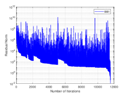
(a) BB1

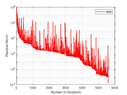
(b) ABB

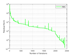
(c) RBB

Figure 1: On performances of BB, ABB and RBB methods for a 100-dimensional problem.

5 Enhanced Regularized Barzilai-Borwein (ERBB) method

In this section, we propose an enhanced RBB (ERBB) stepsize (5.2) which utilizes a diagonal approximation of local Hessian, making it to be applied to both quadratic and general unconstrained optimization problems, and this operation substantially reduces the computational cost and improves the performance of RBB method. Meanwhile, an adaptive alternate stepsize strategy improves the convergence speed of RBB method. Therefore, based on the above two improvements, the overall performance of RBB method is enhanced.

5.1 ERBB method for solving (1.7)

In Section 2, for solving quadratic problems (1.7), we use the Hessian $A$ of objective function $f(x)$ to generate $\alpha_{k}^{RBB}$. Note that equation (1.11) when $\Phi_{1}$=$\Phi_{2}$=$A$, which is equivalent to

$$\alpha_{k}^{RBB}=\frac{s_{k-1}^{\text{T}}y_{k-1}+\tau_{k}y_{k-1}^{\text{T}}Ay_{k-1}}{s_{k-1}^{\text{T}}s_{k-1}+\tau_{k}y_{k-1}^{\text{T}}y_{k-1}}.$$ (5.1)

On one hand, calculating the local Hessian is very expensive if objective function is not quadratic. On the other hand, even for quadratic objective functions, the matrix-vector multiplication increases the computational cost substantially as the size of problem becomes large. And from the inequalities (2.6), we know that the term $\frac{y_{k-1}^{\text{T}}Ay_{k-1}}{y_{k-1}^{\text{T}}y_{k-1}}$ may cause the $\alpha_{k}^{RBB}$ to be too large, i.e., it leads to a too short stepsize, which affects the actual convergence speed of RBB method. To overcome these defects, combining the analysis in Section 2 and the $\alpha_{k}^{RBB}$ in (5.1), we take

$$\alpha_{k}^{RBBnew}=\frac{s_{k-1}^{\text{T}}y_{k-1}+\tau_{k}y_{k-1}^{\text{T}}\Phi_{k}y_{k-1}}{s_{k-1}^{\text{T}}s_{k-1}+\tau_{k}y_{k-1}^{\text{T}}y_{k-1}},$$ (5.2)

where the diagonal matrix

$$\Phi_{k}=\small{\begin{pmatrix}\phi_{k}&&\\ &\ddots&\\ &&\phi_{k}\end{pmatrix}}\in\mathbb{R}^{n\times n},$$ (5.3)

where the diagonal elements

$$\phi_{k}=\max\{\alpha_{j}^{BB2}|j\in\{j_{0},\,\ldots,\,k\}\}$$

with $j_{0}=\max\{1,\,k-moo\}$, $moo\geq 0$ is an integer. In the case of $moo=0$, because of the basic inequality [26], we have that

$$\alpha_{k}^{BB1}\leq\alpha_{k}^{RBBnew}\leq\alpha_{k}^{BB2}$$ (5.4)

holds in (5.2). Similarly, in the case of $moo\geq 1$, we have

$$\alpha_{k}^{BB1}\leq\alpha_{k}^{RBBnew}\leq\phi_{k}\leq\lambda_{n},$$ (5.5)

where $\lambda_{n}$ is the largest eigenvalue of $\nabla^{2}f(x_{k})$. Therefore, $\alpha_{k}^{RBBnew}$ remains within the spectrum of $\nabla^{2}f(x_{k})$, but the latter is a bit more extensive. The diagonal matrix $\Phi_{k}$ in (5.3) is an effective approximation to the local Hessian of objective function at the $k$th iteration with suitable parameter $moo$. Other Hessian approximations $\Phi_{k}$ can also be used in (5.2), but the one presented here appears to the most successful in practice [40]. The success of adaptive schemes [51, 25] inspired us to use the following adaptively alternate stepsize scheme

$$\alpha_{k}^{ERBB}=\begin{cases}\max\{\alpha_{j}^{RBBnew}|j\in\{j_{0},\,\ldots,\,k\}\},&\text{if}\quad\alpha_{k}^{BB1}/\alpha_{k}^{BB2}<\nu_{k},\\ \alpha_{k}^{BB1},&\text{otherwise},\end{cases}$$ (5.6)

where $j_{0}=\max\{1,\,k-mu\}$, $mu>0$ is an integer,

$$\nu_{k}=1-\frac{\alpha_{k}^{BB1}}{\alpha_{k}^{RBBnew}}\in(0,1).$$ (5.7)

As shown in ABB scheme (4.2), if the $\alpha_{k}^{BB1}/\alpha_{k}^{BB2}$ is close to $1$, it means that the $-g_{k-1}$ is a good descent direction, and choosing $\alpha_{k}^{BB1}$ can speed up convergence; otherwise, $\max_{j_{0}\leq j\leq k}\{\alpha_{j}^{RBBnew}\}$ is selected. Specifically, if $\alpha_{k}^{BB1}/\alpha_{k}^{BB2}\geq\nu_{k}$, then $\alpha_{k}^{BB1}/\alpha_{k}^{BB2}\geq 0.5$ and $\alpha_{k}^{BB1}/\alpha_{k}^{RBBnew}\geq 0.5$ hold. This implies that $-g_{k-1}$ is a favorable descent direction; otherwise, $-g_{k-1}$ is not a favorable descent direction. The adaptive alternate stepsize scheme is used to accelerate the convergence of the RBB method, i.e., we choose $\alpha_{k}^{BB1}$ only if $g_{k-1}$ is close to one of the eigenvectors of $A$. For the quadratic optimization problems (1.7), the $R$-linear global convergence of the ERBB method (5.6) can be easily established using the property in [13]. Therefore, we will not repeat it here.

Remark 5.1

Since the ERBB method with adaptive regularization parameter (4.3) can lead to produce a good descent direction, which means that the $\alpha_{k}^{BB1}$ in the alternate stepsize strategy (5.6) can approximate eigenvalues $\lambda$ of $A$ properly, the ERBB method (5.6) can improve the convergence speed of RBB method.

Observing (5.2), the ERBB method seems to require one more inner product per iteration than BB methods, but this extra computational work can be eliminated by using following formulas:

$$s_{k-1}^{\text{T}}s_{k-1}=t_{k-1}^{2}g_{k-1}^{\text{T}}g_{k-1},\,s_{k-1}^{\text{T}}y_{k-1}=t_{k-1}g_{k-1}^{\text{T}}(g_{k-1}-g_{k}),\,y_{k-1}^{\text{T}}y_{k-1}=g_{k}^{\text{T}}g_{k}-2g_{k-1}^{\text{T}}g_{k}+g_{k-1}^{\text{T}}g_{k-1},$$ (5.8)

where $t_{k-1}=\frac{1}{\alpha_{k-1}^{ERBB}}$. Notice that at every iteration, we only need to compute two inner products, i.e., $g_{k-1}^{\text{T}}g_{k}$ and $g_{k}^{\text{T}}g_{k}$. Our extensive numerical experiments show that these formulas are reliable in the quadratic case. For non-quadratic functions, there might be negative or zero denominators, which could also happen while using the original formulas. In this case, we use the above formulas to calculate $\frac{\|s_{k-1}\|_{2}}{\|y_{k-1}\|_{2}}$ as stepsize .

We apply the ERBB method to construct Algorithm 2 for finding the optimal solution to problem (1.7).

Input: Stopping criterion: $\varepsilon>0$, ${\text{MaxIt}>0}$;

Initialization: $A$, $b$, $k=1$, $x_{1}$, Regularization parameter: $\tau_{1}=0$; initial stepsize $t_{1}$;

1 while $k<{\rm{MaxIt}}$ and $\min\left\{\|x_{k+1}-x_{k}\|_{2},\,\frac{\|g_{k}\|_{2}}{\|g_{0}\|_{2}}\right\}>\varepsilon$ do

2      compute $t_{k}=\frac{1}{\alpha_{k}^{ERBB}}$ by (5.6) with adaptive parameter $\tau_{k}$ (4.3).

3       $x_{k+1}=x_{k}-t_{k}g_{k}$,  evaluate $g_{k+1}$.

4       $k=k+1$.

5 end while

Algorithm 2 ERBB: Enhanced Regularized Barzilai-Borwein algorithm for solving (1.7)

5.2 ERBB method for solving (1.1)

To extend ERBB method for minimizing general objective functions (1.1), we usually need to incorporate some line search to ensure global convergence. Among BB-like methods, nonmonotone line search is an effective strategy [31, 9, 4]. Here we would like to adopt the Grippo-Lampariello-Lucidi (GLL) nonmonotone line search [30], which accepts $\gamma_{k}$ when it satisfies

$$f(x_{k}+\gamma_{k}d_{k})\leq\max_{1\leq j\leq\min\{k,\,M-1\}}\{f(x_{k-j})\}+\sigma\gamma_{k}g_{k}^{\text{T}}d_{k},$$ (5.9)

where $\sigma\in(0,\,1)$ is a parameter, $d_{k}$ is a descent direction. In order to obtain global convergence for BB method, this nonmonotone line search strategy was first combined with BB method by Raydan [42] in 1997.

The combination of the gradient method with the stepsize formula (5.6) and the GLL nonmonotone line search strategy (5.9) yields a new algorithm, named Algorithm 3. Under some standard assumptions, global convergence of Algorithm $3$ can similarly be established and the convergence rate is $R$-linear for strongly convex objective functions [42]. Similarly, the equations in (5.1) can be used in Algorithm 3, thus reducing the computational cost.

Input: stopping criterion: $\varepsilon>0$, ${\text{MaxIt}>0}$;

Initialization: $x_{1}\in\mathbb{R}^{n}$, $t_{\rm{max}}\geq t_{\rm{min}}>0$, initial stepsize $t_{1}\in[t_{\text{min}},\,t_{\text{max}}]$, $\sigma$, $\delta\in(0,\,1)$, $M,moo,mu\in\mathbb{N}$, $k:=1$, regularization parameter: $\tau_{1}=0$.

1 while $k<\rm{MaxIt}$ and $\min\left\{\|x_{k+1}-x_{k}\|_{2},\,\frac{\|g_{k}\|_{2}}{\|g_{1}\|_{2}}\right\}>\varepsilon$ do

2      $d_{k}=-t_{k}g_{k}$, $\gamma_{k}=t_{k}$, $f_{r}=\max_{1\leq j\leq\min\{k,\,M-1\}}\{f(x_{k-j})\}$.

3       while the condition (5.9) does not hold do

4            $\gamma_{k}=\delta\gamma_{k}$.

5       end while

6      $x_{k+1}=x_{k}+\gamma_{k}d_{k}$.

7       if $s_{k}^{\text{T}}y_{k}>0$ then

8             compute $\tau_{k}$ by (4.3), $t=\frac{1}{\alpha_{k}^{ERBB}}$ by (5.6).

9      else

10            $\bar{bb}=\frac{\|s_{k}\|_{2}}{\|y_{k}\|_{2}}$, $t_{k}=\min(\bar{bb},\,\frac{1}{\|g_{k}\|_{\infty}})$.

11       end if

12      $t_{k}=\max\{t_{\text{min}},\,\min\{t_{k},\,t_{\text{max}}\}\}$.

13       $k=k+1$.

14 end while

Algorithm 3 ERBB: Enhanced Regularized Barzilai-Borwein algorithm for solving (1.1)

6 Numerical experiments

In this section, we present some numerical results to verify the analysis in the preceding sections. Since we are mainly concerned with the effect of regularization on original BB stepsize, it is only tested for numerical comparison with BB-like methods. Here, BB1 method refers to the method with BB1 stepsize, and BB2 method refers to the method with BB2 stepsize. In the next two subsections, the numerical results of Algorithm 2 and Algorithm 3 are presented separately for quadratic functions (1.7) and general objective functions (1.1).

We report the number of iterations (Iter), CPU times in seconds (Time). All numerical experiments performed using Matlab R2019a under a Windows 11 operating system on a DELL G15 5200 personal computer with an Intel Core i7-12700H and 16 GB of RAM.

6.1 Performance comparison on the problems (1.7)

First, we test Algorithm 1 to examine the performance of regularization parameters $\tau_{k}(r)$ in (4.12) with different $r$ in problem (4.13). We set $n=100$, the initial point $x_{0}=(x_{0}^{(1)},\ldots,x_{0}^{(n)})^{\text{T}}\in\mathbb{R}^{n}$ and $x_{*}=(x_{*}^{(1)},\ldots,x_{*}^{(n)})^{\text{T}}\in\mathbb{R}^{n}$, where $x_{0}^{(i)}\in[-1,1]$ and $x_{*}^{(i)}\in[-1,1]$ are randomly generated, $i=1,2,\ldots,n$, the termination condition is $\|g_{k}\|_{2}\leq 10^{-10}\|g_{0}\|_{2}$. Running independently $20$ times, Table 1 reports the average number of iterations when the program meets the termination condition under different condition number $\kappa$ of $A$ and different $r$.

Table 1: Performance of regularization parameters with different $r$ in problem (4.13).

	0.5	1	1.5	2	2.5	3	3.5	4
1.00E+04	1149.2	1110.3	979.5	990.9	1035.8	1038.9	1026.3	1088.8
1.00E+05	1677	1746.8	1897.3	1941.3	2123.2	2287.8	2351.9	2530.3
1.00E+06	2199.4	2201.3	2389.3	2668.2	3094.1	3641.6	3770.3	4118.7
1.00E+07	2709.6	2860.3	2750.3	2896.3	3673	3943.6	4327.4	5466.9
1.00E+08	3562.6	3456.3	3166.8	3440	3950.3	4544.3	5400.7	5946.3

Observing the results in Table 1, we see that the impact of $r$ on $\tau_{k}(r)$ in (4.12) is not significant when the condition number $\kappa=10^{4}$. As the condition number increases, $r$ increases from $1.5$ to $4$, and the average number of iterations also increases. The average number of iterations is generally consistent when $r$ is taken as $0.5$, $1$ and $1.5$. Therefore, we take $r=1$ in the later tests, but we can also see that $r=0.5$ or $1.5$ has an advantage in some problems.

We test Algorithm 2 on some randomly generated quadratic problems. The objective function is given by

$$f(x)=(x-x^{*})^{\text{T}}A(x-x^{*}),$$ (6.1)

where $x^{*}$ was randomly generated with components in $[-10,\,10]$, the matrix $A=\text{diag}(v_{1},\,v_{2},\,\ldots,\,v_{n})$ is a diagonal matrix with nonzero elements $v_{1}=1$ and $v_{n}=\kappa$, and $v_{j}$, $j=2,\,\ldots,\,n-1$, being randomly generated between $1$ and $\kappa$. Further, we investigate the performance of Algorithm 2 for quadratic forms (6.1) with different spectral distributions. Table 2 lists seven types of diagonal matrices with different spectral distributions, which derived from [15, 32].

Table 2: Distributions of $v_{i}$.

Set	Spectrum	Set	Spectrum
P1	$\{v_{2},\ldots,v_{n-1}\}\subset(1,\kappa)$	P5	$\{v_{2},\ldots,v_{n/5}\}\subset(1,\zeta)$
P2	$\{v_{2},\ldots,v_{n/5}\}\subset(1,\zeta)$		$\{v_{n/5+1},\ldots,v_{4n/5}\}\subset(\zeta,\frac{\kappa}{2})$
	$\{v_{n/5+1},\ldots,v_{n-1}\}\subset(\frac{\kappa}{2},\kappa)$		$\{v_{4n/5+1},\ldots,v_{n-1}\}\subset(\frac{\kappa}{2},\kappa)$
P3	$\{v_{2},\ldots,v_{n/2}\}\subset(1,\zeta)$	P6	$\{v_{2},\ldots,v_{10}\}\subset(1,\zeta)$
	$\{v_{n/2+1},\ldots,v_{n-1}\}\subset(\frac{\kappa}{2},\kappa)$		$\{v_{11},\ldots,v_{n-1}\}\subset(\frac{\kappa}{2},\kappa)$
P4	$\{v_{2},\ldots,v_{4n/5}\}\subset(1,\zeta)$	P7	$\{v_{2},\ldots,v_{n-10}\}\subset(1,\zeta)$
	$\{v_{4n/5+1},\ldots,v_{n-1}\}\subset(\frac{\kappa}{2},\kappa)$		$\{v_{n-9},\ldots,v_{n-1}\}\subset(\frac{\kappa}{2},\kappa)$

We use the following stopping condition

$$\|g_{k}\|_{2}\leq\varepsilon\|g_{0}\|_{2},$$

or the number of iterations exceeds MaxIt $20,000$. Initial stepsize is $t_{0}=\frac{1}{\alpha_{0}^{SD}}=\frac{g_{0}^{\text{T}}g_{0}}{g_{0}^{\text{T}}Ag_{0}}$, which is the stepsize in the steepest descent method. In this test, we take $\varepsilon=10^{-9},\,10^{-12},\,10^{-15}$, $10^{-18}$, and $\kappa=10^{5},\,10^{6},\,10^{7},\,10^{8},\,10^{9}$, $n=100,\,1000$, respectively. In Table 2, we take $\zeta=999$ for the test. For each value of $\kappa$ and $\varepsilon$, $10$ different starting points with entries in $[-5,\,5]$ were randomly generated. In ERBB method (5.6), the parameters $moo$ and $mu$ are taken as $6$ and $7$, respectively.

To further illustrate the efficiency of Algorithm 2 for quadratic problems, we compare it with following superior BB-like methods:

1. BB1[7]: the original BB method using $\alpha_{k}^{BB1}$;

2. BB2[7]: the original BB method using $\alpha_{k}^{BB2}$;

3. ABB[51]: the adaptive BB method;

4. ABBmin[25]: a gradient method adaptively uses $\alpha_{k}^{BB1}$ and $\max\{\alpha_{j}^{BB2}:\,j=\max\{\{1,\,k-m\},\ldots,\,k\}\}$;

5. BBQ[31]: a BB method with two-dimensional quadratic termination property.

We use the same initial point, condition number and tolerance as before. As suggested in [25, 31], $\nu_{k}=0.15,\,0.5$ were used in ABB, ABBmin methods, respectively, and $m=9$ was used for ABBmin method, $\nu_{1}=0.2$, $\gamma=1.02$ were employed in BBQ method.

We present in Figure 2 a $\text{log}_{2}$ scaled view of the performance profiles [22, 44] obtained by the Algorithm 2 and other methods using the number of iterations as the metric. There are altogether $7\times 5\times 4\times 10\times 2=2800$ randomly generated quadratic problems. For each method, the vertical axis of the figure shows the percentage of problems the method solves within the factor $\omega$ of the minimum value of the metric. It can be seen that Algorithm 2 clearly outperforms other compared methods.

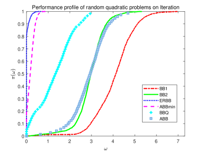
Figure 2: Performance profiles of Algorithm 2, BB1, BB2, ABB, ABBmin, BBQ methods on random quadratic problems (6.1) for dimensions of $n=100,1000$ with spectral distribution in Table 2.

Table 3 presents the average CPU time and number iterations required by the compared methods to meet given tolerances. We see that ERBB method with adaptive parameter has advantages on most of the problems.

Table 3: Performance of different methods on quadratic problems.

n=1000			BB1		BB2		ERBB		ABBmin		BBQ		ABB
P	$\kappa$	$\varepsilon$	Time	Iter	Time	Iter	Time	Iter	Time	Iter	Time	Iter	Time	Iter
P1	$10^{5}$	$10^{-9}$	0.171	1748.5	0.159	1731.5	0.018	199.3	0.021	218.3	0.029	292.9	0.041	389.9
		$10^{-12}$	0.957	3353.0	0.695	2204.5	0.075	229.7	0.080	236.3	0.141	441.6	0.256	782.6
		$10^{-15}$	1.841	3436.7	1.162	2020.3	0.132	242.9	0.142	255.7	0.306	507.6	0.389	566.9
		$10^{-18}$	1.796	3315.7	1.193	2245.7	0.147	262.7	0.164	290.8	0.281	520.9	0.387	703.6
	$10^{9}$	$10^{-9}$	0.063	545.9	0.064	565.8	0.030	271.9	0.031	265.7	0.048	433.0	0.046	446.2
		$10^{-12}$	1.695	3480.3	0.524	1248.1	0.172	395.4	0.179	404.3	0.341	806.1	0.639	1499.3
		$10^{-15}$	2.019	4076.6	0.688	1231.6	0.217	388.9	0.224	395.6	0.467	839.8	0.657	1186.3
		$10^{-18}$	2.257	3974.7	0.662	1145.5	0.231	406.4	0.248	430.5	0.532	832.8	0.827	1444.0
P2	$10^{5}$	$10^{-9}$	1.040	1691.5	0.854	1369.2	0.122	199.2	0.136	217.4	0.435	718.9	0.700	1136.7
		$10^{-12}$	1.437	2261.7	1.102	1737.6	0.159	252.3	0.166	263.7	0.625	982.0	0.838	1316.5
		$10^{-15}$	1.421	2281.0	1.148	1842.4	0.176	282.8	0.182	293.0	0.626	999.8	0.950	1522.4
		$10^{-18}$	1.502	2428.0	1.127	1806.8	0.191	305.2	0.203	322.8	0.711	1127.2	0.926	1479.3
	$10^{9}$	$10^{-9}$	2.532	4886.9	0.756	1488.3	0.037	67.5	0.039	70.7	0.064	116.5	1.122	2071.3
		$10^{-12}$	3.043	4894.4	1.040	1671.0	0.105	169.8	0.104	168.7	0.139	223.0	1.060	1706.3
		$10^{-15}$	3.416	5564.2	1.259	2008.7	0.140	218.4	0.132	198.3	0.217	321.4	0.987	1552.2
		$10^{-18}$	3.510	5557.4	1.087	1722.9	0.162	257.0	0.157	248.1	0.257	415.1	1.303	2072.1
P4	$10^{5}$	$10^{-9}$	1.095	1719.9	1.035	1659.1	0.150	238.1	0.156	250.9	0.563	902.8	0.972	1559.8
		$10^{-12}$	1.540	2439.1	1.047	1632.1	0.187	296.6	0.201	306.1	0.662	1036.9	1.111	1774.5
		$10^{-15}$	1.690	2513.5	1.150	1823.0	0.200	315.7	0.223	352.5	0.736	1182.3	1.157	1854.2
		$10^{-18}$	1.557	2453.5	1.099	1796.6	0.230	361.1	0.229	372.2	0.753	1216.1	1.215	1958.7
	$10^{9}$	$10^{-9}$	2.823	4682.5	0.955	1522.5	0.048	77.5	0.054	84.3	0.083	133.5	1.156	1867.8
		$10^{-12}$	3.593	5853.9	1.050	1705.5	0.113	180.5	0.121	195.1	0.157	252.1	1.317	2135.0
		$10^{-15}$	3.105	5026.6	1.114	1812.7	0.160	255.1	0.166	266.0	0.241	379.8	1.252	2020.9
		$10^{-18}$	3.575	5693.0	1.202	1938.5	0.183	292.2	0.194	311.7	0.299	478.4	1.418	2200.2
P5	$10^{5}$	$10^{-9}$	1.461	2356.0	1.373	2173.2	0.295	461.1	0.299	473.9	1.118	1777.9	1.065	1719.3
		$10^{-12}$	2.293	3821.6	1.670	2759.2	0.293	487.0	0.345	576.8	1.275	2090.5	1.339	2216.2
		$10^{-15}$	2.332	3975.3	1.605	2694.9	0.329	552.5	0.356	593.0	1.286	2165.6	1.294	2227.1
		$10^{-18}$	2.307	3889.4	1.568	2606.8	0.326	549.2	0.358	587.0	1.324	2215.9	1.439	2430.5
	$10^{9}$	$10^{-9}$	7.149	12394.0	3.101	5377.6	0.289	497.1	0.333	575.5	1.716	2977.0	3.018	5215.0
		$10^{-12}$	6.735	11728.0	2.915	5027.9	0.369	621.9	0.388	665.8	1.963	3396.3	3.755	6438.5
		$10^{-15}$	7.883	13755.0	3.305	5758.1	0.394	687.8	0.429	737.6	1.986	3426.7	3.128	5483.1
		$10^{-18}$	7.191	12451.0	3.454	5889.8	0.439	726.6	0.465	797.8	2.094	3581.9	4.855	8362.6

Furthermore, we again compare the above methods for the non-random quadratic problem (4.13). The initial settings and termination conditions of this problem are the same as those in the previous test problems. Table 4 presents the average numerical results of the different methods for $10$ independent runs. From Table 4, we can see that the Algorithm 2 again outperforms the others for all the problems in CPU time and iteration number.

Table 4: Performance of different methods on non-random quadratic problems (4.13) with $n=1000$.

n=1000		BB1		BB2		ERBB		ABBmin		BBQ		ABB
$\kappa$	$\varepsilon$	Time	Iter	Time	Iter	Time	Iter	Time	Iter	Time	Iter	Time	Iter
$10^{5}$	$10^{-9}$	0.57	3003.30	0.47	2736.80	0.10	541.90	0.11	598.80	0.39	2136.70	0.43	2434.40
	$10^{-12}$	2.14	4008.10	1.55	3001.60	0.30	603.80	0.33	674.90	1.31	2632.10	1.43	2956.00
	$10^{-15}$	2.04	3909.70	1.64	3037.70	0.36	665.10	0.40	733.10	1.57	2936.10	1.44	2979.80
	$10^{-18}$	2.23	4251.70	1.52	2908.40	0.36	673.70	0.39	740.60	1.51	2853.90	1.66	3140.00
$10^{6}$	$10^{-9}$	3.91	7422.40	2.35	4453.20	0.37	702.20	0.39	743.10	2.08	3944.50	2.98	5307.90
	$10^{-12}$	4.55	8648.90	2.61	4940.10	0.41	764.00	0.46	875.60	2.33	4414.20	3.01	5679.90
	$10^{-15}$	4.07	7784.70	2.38	4525.70	0.44	803.00	0.49	919.40	2.61	4925.20	3.02	5736.70
	$10^{-18}$	3.50	9130.30	1.68	4826.30	0.31	857.60	0.34	960.80	1.73	4857.60	1.93	5294.70
$10^{7}$	$10^{-9}$	1.43	12105.00	0.71	5803.80	0.11	819.40	0.12	942.90	0.75	5703.40	1.32	7147.80
	$10^{-12}$	6.09	12407.00	2.76	5380.40	0.50	947.60	0.55	1051.70	3.59	6804.10	4.44	8259.90
	$10^{-15}$	6.87	12989.00	2.81	5336.60	0.52	977.70	0.59	1109.30	3.55	6701.50	4.75	8916.10
	$10^{-18}$	6.16	12288.00	3.04	5753.80	0.53	1006.60	0.59	1129.20	3.65	6953.00	4.34	8241.00
$10^{8}$	$10^{-9}$	6.18	13901.00	2.67	5430.40	0.49	927.00	0.58	1097.20	3.86	7290.20	4.61	8798.70
	$10^{-12}$	7.35	14159.00	3.28	6329.60	0.57	1079.10	0.63	1201.60	4.36	8325.40	5.00	9627.50
	$10^{-15}$	7.10	13651.00	3.20	6149.70	0.60	1132.30	0.68	1296.80	4.69	8955.40	5.19	9963.50
	$10^{-18}$	7.45	14203.00	3.64	6898.80	0.64	1194.10	0.73	1361.80	4.71	8655.80	4.95	9844.20
$10^{9}$	$10^{-9}$	6.64	12634.00	3.35	6375.80	0.57	1062.40	0.62	1151.70	4.31	8020.40	5.41	10273.00
	$10^{-12}$	9.18	17390.00	4.19	7972.50	0.63	1188.00	0.74	1417.40	5.16	9721.20	6.42	12926.00
	$10^{-15}$	7.37	15570.00	3.95	8964.60	0.55	1251.90	0.65	1466.80	4.62	10554.00	5.56	12409.00
	$10^{-18}$	7.66	17776.00	4.09	8713.80	0.65	1332.50	0.71	1552.90	4.85	10648.00	7.10	14095.00

6.2 Finding spherical $t$-designs efficiently by ERBB method

In this part, we apply Algorithm 3 to a challenging problem of finding a set of points with “good” distribution on the unit sphere $\mathbb{S}^{2}:=\{(x,y,z)^{\text{T}}\in\mathbb{R}^{3}|x^{2}+y^{2}+z^{2}=1\}$.

A point set $\mathcal{X}=\{\mathtt{x}_{1},\ldots,\mathtt{x}_{N}\}\in\mathbb{S}^{2}$ is a spherical $t$-design if it satisfies

$$\frac{1}{N}\sum_{j=1}^{N}p(\mathtt{x}_{j})=\frac{1}{4\pi}\int_{\mathbb{S}^{2}}p(\mathtt{x})d\omega(\mathtt{x})\quad\quad\forall p\in\mathbb{P}_{t},$$

where $d\omega(\mathtt{x})$ denotes area measure on the unit sphere. That is, $\mathcal{X}$ is a spherical $t$-design if a properly scaled equal-weight quadrature rule with nodes at the points of $\mathcal{X}_{N}$ integrates all (spherical) polynomials up to degree $t$ exactly. For more details on spherical designs, see [20, 1, 6]. In particular, [37] applied the theory of numerical integration formulas with algebraic precision to polynomial optimization.

In the influential paper [43], the authors present a variational characterization of spherical $t$-design as follows

$$A_{N,t}(X_{N}):=\frac{4\pi}{N^{2}}\sum_{n=1}^{t}\sum_{k=1}^{2n+1}(\sum_{i=1}^{N}Y_{n}^{k}(\bm{x}_{i}))^{2}=\frac{4\pi}{N^{2}}\sum_{j=1}^{N}\sum_{i=1}^{N}\sum_{n=1}^{t}\frac{2n+1}{4\pi}P_{n}(\langle\bm{x}_{j},\bm{x}_{i}\rangle),$$ (6.2)

where $Y_{n}^{k}$ are the orthonormal real spherical harmonics basis of degree $n$ and order $k$ for $\Pi_{t}$, $P_{n}:[-1,1]\rightarrow\mathbb{R}$ is Legendre polynomial [8] and $\langle\bm{x},\bm{y}\rangle:=\bm{x}^{\text{T}}\bm{y}$ is the inner product in $\mathbb{R}^{3}$. It is know that $X_{N}$ is a spherical $t$-design if and only if $A_{N,t}(X_{N})=0$ [43]. Therefore, the problem of finding a spherical $t$-design is expressed as solving a nonlinear and non-convex optimization problem:

$$\min_{X_{N}\subset{\mathbb{S}^{2}}}A_{N,t}(X_{N}).$$ (6.3)

For solving the optimization problem (6.3), [4] numerically construct spherical $t$-designs by using BB1 method. Based on the code in [4], we perform numerical experiments of BB1 and ERBB methods. Here we set $\varepsilon_{1}=10^{-8}$, $\varepsilon_{2}=10^{-16}$ as termination tolerance on the first-order optimality and function value changes, respectively. That is the termination condition of the algorithms is as follows

$$\|g_{k}\|_{2}<\varepsilon_{1}\quad\text{or}\quad|f_{k}-f_{k-1}|<\varepsilon_{2}\quad\text{or}\quad\|x_{k}-x_{k-1}\|_{2}<\varepsilon_{2},$$

The maximum number of iterations and function evaluations are $10^{4}$ and one million. In Algorithm 3, we set $moo=6$, $mu=7$, $t_{min}=10^{-20}$, $t_{max}=10^{10}$ and use non-monotone line search strategy with $\sigma=10^{-4}$, $\delta=0.5$, initial stepsize $t_{1}=1$. In the BB1 method, the parameters in [4] are used by default. The initial points in this experiment are consistent with those in [4].

We report in Table 5 the number of iterations, function values $A_{N,t}(X_{N})$, gradient norms $\|\nabla^{*}A_{N,t}\|_{2}$, and CPU time costs of the BB1 and ERBB methods when the termination conditions are met for different $t$ on $\mathbb{S}^{2}$. The variational characterization (6.2) of spherical $t$-design varies very much for different $t$. We observe that except for $t=10,50,65,99$, ERBB takes less CPU time than BB1 method on the rest of the problems, especially on large $X_{N}$. Meanwhile, we notice that ERBB obtains higher-precision solutions at $t=50,65,99$. In general, as $t$ increases, that is, as the problem size continues to increase, the effect of ERBB becomes more significant. Figure 3 and Figure 4 show the behavior of $\|\nabla A_{N,t}(X_{N})\|_{2}$ for BB1 and ERBB methods in different problems, corresponding to a varying $t$ from $20$ to $127$. We can observe that in these problems, the ERBB and BB1 methods perform similarly at the beginning of the iteration, after which ERBB method shows faster convergence. This verifies that ERBB does not destroy the global convergence of the BB1 method at the early stage of the iteration (i.e., the iterate is far away from the optimal solution), and the parameters in ERBB method do make excellent use of the local nature (curvature) of the objective function, which enables faster convergence.

Table 5: Computing of Spherical $t$-designs by BB1 and ERBB Methods

Problem		BB1				ERBB
t	N	Iteration	$A_{N,t}(X_{N})$	$\|\nabla^{*}A_{N,t}(X_{N})\|_{2}$	Time	Iteration	$A_{N,t}(X_{N})$	$\|\nabla^{*}A_{N,t}(X_{N})\|_{2}$	Time
10	121	100	1.28E-15	1.17E-08	0.1668	103	5.38E-15	1.96E-08	0.174
15	169	132	5.33E-15	3.37E-08	0.6223	123	5.55E-16	8.89E-09	0.5896
20	441	253	6.56E-16	1.86E-07	2.8923	173	9.82E-16	5.95E-09	2.0194
25	676	241	1.00E-13	2.41E-08	5.3553	202	4.89E-13	5.39E-08	4.5828
30	961	274	3.05E-14	1.11E-08	11.35	211	1.08E-12	6.98E-08	8.7998
35	1296	437	1.11E-12	6.01E-08	35.048	288	1.53E-13	5.04E-08	22.585
40	1681	821	7.23E-15	1.33E-08	125.1784	388	8.07E-15	8.64E-09	52.1116
45	2116	1842	2.49E-13	2.64E-08	509.9561	369	5.77E-14	1.91E-08	84.0232
50	2601	375	1.14E-13	1.90E-08	131.5703	378	2.94E-14	1.02E-08	143.056
55	3136	444	6.22E-13	3.15E-08	337.7956	352	7.34E-13	5.03E-08	260.5626
60	3721	390	6.26E-12	9.92E-08	389.3074	319	2.49E-12	9.78E-08	324.3694
65	4356	673	6.14E-14	2.52E-08	1.09E+03	473	3.00E-15	8.79E-09	1.12E+03
70	5041	598	3.76E-13	3.66E-08	2.76E+03	328	7.07E-12	1.15E-07	1.61E+03
75	5776	568	7.00E-16	1.53E-08	3.02E+03	457	2.63E-14	1.50E-08	2.37E+03
80	6561	1097	1.15E-11	9.07E-08	7.53E+03	493	1.31E-13	1.18E-08	3.24E+03
84	7225	605	8.41E-13	1.20E-07	6.77E+03	529	2.17E-15	8.72E-09	4.60E+03
88	7921	1126	6.26E-12	5.79E-08	1.24E+04	511	4.84E-12	6.56E-08	5.57E+03
90	8281	2310	1.07E-11	8.21E-08	2.41E+04	1644	4.51E-12	6.12E-08	2.20E+04
99	10000	339	2.04E-09	1.06E-06	6.15E+03	691	1.07E-11	6.76E-08	1.46E+04
127	16384	3296	8.81E-12	7.59E-08	2.72E+05	776	1.47E-11	7.72E-08	5.64E+04

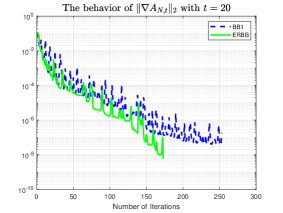
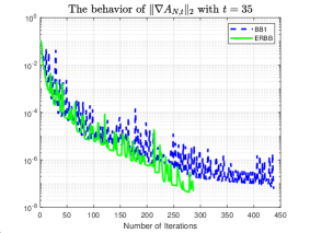
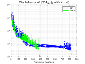
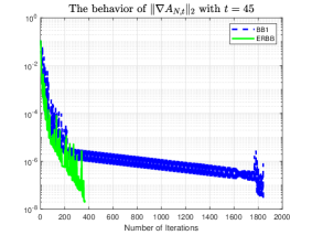
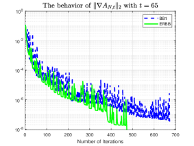
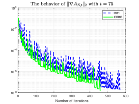
Figure 3: The behavior of $\nabla A_{N,t}$ for different $t$, $N=(t+1)^{2}$ on $\mathbb{S}^{2}$ by BB1 and ERBB methods.

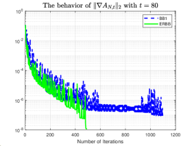
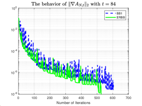
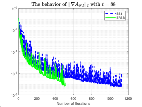
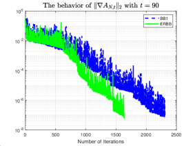
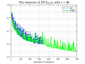
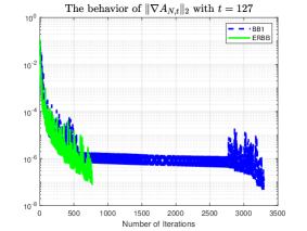
Figure 4: The behavior of $A_{N,t}$ for different $t$ on $\mathbb{S}^{2}$ by BB1 and ERBB methods.

7 Concluding remarks

In this paper, we propose a regularized Barzilai-Borwein stepsize for solving some ill-conditioned problems and analyze the convergence and stability of RBB algorithm. And for general optimization problems, we propose an enhanced RBB method. The enhanced RBB method improves the efficiency of original RBB method by a diagonal matrix that approximates the Hessian of objective function, reducing the computational cost, and an adaptive alternate stepsize strategy. Combing a global stabilized operation, we theoretically establish the global convergence and local R-linear convergence rate of the enhanced RBB method for quadratic and general optimization problems, respectively. We preliminarily discuss the selection of regularization parameters and obtain one scheme for adaptive generation of regularization parameters using adjacent old stepsizes. Some numerical experiments verify the performance of the enhanced RBB method with adaptive regularization parameter. However, the selection of more appropriate regularization parameters and the relationship between the performance of regularized Barzilai-Borwein method and the spectral distribution of local Hessian still need to be further explored.

References

• [1] C. An, X. Chen, I. H. Sloan, and R. S. Womersley, Well Conditioned Spherical Designs for Integration and Interpolation on the Two-Sphere, SIAM Journal on Numerical Analysis, 48 (2010), p. 2135–2157.
• [2] C. An and H. Wu, Tikhonov regularization for polynomial approximation problems in Gauss quadrature points, Inverse Problems, 37 (2020), pp. 1–20.
• [3] C. An, H. Wu, and X. Yuan, The springback penalty for robust signal recovery, Applied and Computational Harmonic Analysis, 1 (2022), pp. 1–29.
• [4] C. An and Y. Xiao, Numerical construction of spherical t-designs by Barzilai-Borwein method, Applied Numerical Mathematics, 150 (2020), pp. 295–302.
• [5] L. Armijo, Minimization of functions having Lipschitz continuous first partial derivatives, Pacific Journal of Mathematics, 16 (1966), pp. 1–3.
• [6] E. Bannai and E. Bannai, A survey on spherical designs and algebraic combinatorics on spheres, European Journal of Combinatorics, 30 (2009), p. 1392–1425.
• [7] J. Barzilai and J. M. Borwein, Two-point step size gradient methods, IMA Journal on Numerical Analysis, 8 (1988), pp. 141–148.
• [8] R. Beals and R. Wong, Special Functions and Orthogonal Polynomials, Cambridge University Press, May 2016.
• [9] I. Bruno and P. Margherita, The Riemannian Barzilai-Borwein method with nonmonotone line search and the matrix geometric mean computation, IMA Journal of Numerical Analysis, 38 (2015), pp. 495–517.
• [10] O. Burdakov, Y. Dai, and N. Huang, Stabilized Barzilai-Borwein Method, Journal of Computational Mathematics, 37 (2019), pp. 916–936.
• [11] S. Crisci, F. Porta, V. Ruggiero, and L. Zanni, Spectral Properties of Barzilai–Borwein Rules in Solving Singly Linearly Constrained Optimization Problems Subject to Lower and Upper Bounds, SIAM Journal on Optimization, 30 (2020), pp. 1300–1326.
• [12] S. Crisci, V. Ruggiero, and L. Zanni, Steplength selection in gradient projection methods for box-constrained quadratic programs, Applied Mathematics and Computation, 356 (2019), pp. 312–327.
• [13] Y. Dai, Alternate step gradient method, Optimization, 52 (2003), pp. 395–415.
• [14] Y. Dai and R. Fletcher, Projected Barzilai-Borwein methods for large-scale box-constrained quadratic programming, Numerische Mathematik, 100 (2005), pp. 21–47.
• [15] Y. Dai, Y. Huang, and X. W. Liu, A family of spectral gradient methods for optimization, Computational Optimization and Applications, 74 (2019), pp. 43–65.
• [16] Y. Dai and L. Liao, R-linear convergence of the Barzilai and Borwein gradient method, IMA Journal of Numerical Analysis, 22 (2002), pp. 1–10.
• [17] Y. Dai, J. Yuan, and Y. X. Yuan, Modified Two-Point Stepsize Gradient Methods for Unconstrained Optimization, Computational Optimization and Applications, 22 (2002), pp. 103–109.
• [18] Y. Dai and Y. Yuan, Alternate minimization gradient method, IMA Journal of Numerical Analysis, 23 (2003), pp. 1–17.
• [19] R. De Asmundis, D. di Serafino, W. W. Hager, G. Toraldo, and H. Zhang, An efficient gradient method using the Yuan steplength, Computational Optimization and Applications, 59 (2014), p. 541–563.
• [20] P. Delsarte, J. M. Goethals, and J. J. Seidel, Spherical codes and designs, Geometry and Combinatorics, 6 (1977), pp. 363–388.
• [21] A. Dhamacharoen, An efficient hybrid method for solving systems of nonlinear equations, Journal of Computational and Applied Mathematics, 263 (2014), pp. 59–68.
• [22] E. D. Dolan and J. J. Moré, Benchmarking optimization software with performance profiles, Mathematical Programming, 91 (2002), pp. 201–213.
• [23] G. Ferrandi, M. E. Hochstenbach, and N. Krejić, A harmonic framework for stepsize selection in gradient methods, Computational Optimization and Applications, 85 (2023), p. 75–106.
• [24] R. Fletcher, On the Barzilai-Borwein Method, in Optimization and Control with Applications, L. Qi, K. Teo, and X. Yang, eds., Boston, MA, 2005, Springer US, pp. 235–256.
• [25] G. Frassoldati, L. Zanni, and G. Zanghirati, New adaptive stepsize selections in gradient methods, Journal of Industrial and Management Optimization, 4 (2008), pp. 299–312.
• [26] S. Furuichi, Advances in Mathematical Inequalities, De Gruyter, Berlin, 2nd ed., 2020.
• [27] A. A. Goldstein, Cauchy’s method of minimization, Numerische Mathematik, 4 (1962), pp. 146–150.
• [28] G. H. Golub, P. C. Hansen, and D. P. O’Leary, Tikhonov Regularization and Total Least Squares, SIAM Journal on Matrix Analysis and Applications, 21 (1999), pp. 185–194.
• [29] G. H. Golub and C. F. Van Loan, Matrix computations, The Johns Hopkins University Press, Baltimore, 4th ed., 2013.
• [30] L. Grippo, F. Lampariello, and S. Lucidi, A Nonmonotone Line Search Technique for Newton’s Method, SIAM Journal on Numerical Analysis, 23 (1986), pp. 707–716.
• [31] Y. Huang, Y. Dai, and X. Liu, Equipping the Barzilai–Borwein Method with the Two Dimensional Quadratic Termination Property, SIAM Journal on Optimization, 31 (2021), pp. 3068–3096.
• [32] Y. Huang, Y. Dai, X. Liu, and H. Zhang, Gradient methods exploiting spectral properties, Optimization Methods and Software, 35 (2020), pp. 681–705.
• [33] D. Li and R. Sun, On a Faster R-Linear Convergence Rate of the Barzilai-Borwein Method, ArXiv, abs/2101.00205 (2021), pp. 1–11.
• [34] S. Lu and S. V. Pereverzev, Regularization Theory for Ill-posed Problems: Selected Topics, De Gruyter, 2013.
• [35] S. Lu, S. V. Pereverzev, and R. Ramlau, An analysis of Tikhonov regularization for nonlinear ill-posed problems under a general smoothness assumption, Inverse Problems, 23 (2006), pp. 217–230.
• [36] R. Marcos, The Barzilai and Borwein Gradient Method for the Large Scale Unconstrained Minimization Problem, SIAM Journal on Optimization, 7 (1997), pp. 26–33.
• [37] A. Martinez, F. Piazzon, A. Sommariva, and M. Vianello, Quadrature-based polynomial optimization, Optimization Letters, 14 (2019), p. 1027–1036.
• [38] H. Mohammad, Barzilai-Borwein-Like Method for Solving Large-Scale Non-Linear Systems of Equations, Nigerian Mathematical Society, 35 (2017), pp. 71–83.
• [39] J. Nocedal, Theory of algorithms for unconstrained optimization, Acta Numerica, 1 (1992), pp. 199–242.
• [40] J. Nocedal and S. J. Wright, Numerical Optimization, Springer, New York, 2nd ed., 2006.
• [41] M. Raydan, On the Barzilai and Borwein choice of steplength for the gradient method, IMA Journal of Numerical Analysis, 13 (1993), pp. 321–326.
• [42] M. Raydan, The Barzilai and Borwein Gradient Method for the Large Scale Unconstrained Minimization Problem, SIAM Journal on Optimization, 7 (1997), pp. 26–33.
• [43] I. H. Sloan and R. S. Womersley, A variational characterisation of spherical designs, Journal of Approximation Theory, 159 (2009), pp. 308–318. Special Issue in memory of Professor George G. Lorentz (1910–2006).
• [44] A. Z. M. Sofi, M. Mamat, S. Z. Mohid, M. A. H. Ibrahim, and N. Khalid, Performance Profile Comparison Using Matlab, 2015.
• [45] W. Sun and Y. Yuan, Optimization Theory and Methods: Nonlinear Programming, vol. 1, Springer, New York, 2006.
• [46] M. N. Vrahatis, G. S. Androulakis, J. N. Lambrinos, and G. D. Magoulas, A class of gradient unconstrained minimization algorithms with adaptive stepsize, Journal of Computational and Applied Mathematics, 114 (2000), p. 367–386.
• [47] Y. Wang and S. Ma, Projected Barzilai-Borwein Methods for Large Scale Nonnegative Image Restorations, Inverse Problems in Science and Engineering, 15 (2007), pp. 559–583.
• [48] Y. Wang and Y. Yuan, Convergence and regularity of trust region methods for nonlinear ill-posed inverse problems, Inverse Problems, 21 (2005), pp. 821–838.
• [49] P. Wolfe, Convergence Conditions for Ascent Methods, SIAM Review, 11 (1969), pp. 226–235.
• [50] Y. X. Yuan, Non-Monotone Properties and Monotone Properties of Barzilai-Borwein method, tech. rep., Comput. Math. and Scientific/Engineering Computing AMSS, CAS, 2018.
• [51] B. Zhou, L. Gao, and Y. Dai, Gradient Methods with Adaptive Step-Sizes, Computational Optimization and Applications, 35 (2006), pp. 69–86.