Spin Nematic Liquid of the S=1/2 Distorted Diamond Spin Chain in Magnetic Field

Abstract

The magnetization process of the $S=1/2$ distorted diamond spin chain with the anisotropic ferromagnetic interaction is investigated using the numerical diagonalization of finite-size clusters. It is found that the spin nematic and SDW Tomonaga-Luttinger liquids can appear for sufficiently large easy axis anisotropy.

I Introduction

The spin nematic state is one of interesting phenomena in the field of the magnetism. It had been theoretically predicted to appear in the quantum spin systems with the biquadratic interaction or the spin frustration.andreev ; chen ; sudan ; hikihara Recently another mechanism of the spin nematic liquid based on the anisotropy was proposed and it was predicted to occur in the spin ladder and the bond-alternating chain, using the numerical diagonalization analyses.sakai2010 ; sakai2020 ; sakai2021 ; sakai2022 ; sakai2022a ; nakanishi . In this paper, we propose the spin nematic liquid phase in the distorted diamond chain based on the same mechanism.

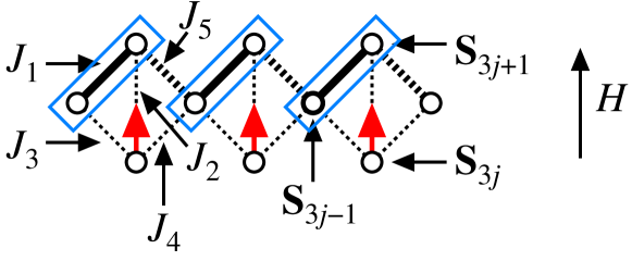
Figure 1: The model of the $S=1/2$ distorted diamond spin chain. Thick solid lines represent $J_{1}<0$, thin dotted lines $J_{2}=J_{3}=J_{4}>0$, and thick dotted lines $J_{5}>0$. Blue rectangles and red arrows are for the explanation of the field-induced spin nematic Tomonaga-Luttinger state (see text).

The distorted diamond chain is the theoretical model of the compound Cu₃(CO₃)₂(OH)₂, called azurite.kikuchi ; okamoto1 ; okamoto2 In this compound all the exchange interaction are antiferromagnetic and it exhibits the 1/3 magnetization plateau due to the trimer nature. Recently other candidate materials for the distorted diamond spin chain were discovered. They are the compound K₃Cu₃AlO₂(SO₄)₄, called alumoklyuchevskitefujihara ; morita ; fujihala2 and related materials. This compound is also a frustrated system, but it includes some ferromagnetic interactions. Thus now we consider the distorted diamond chain including ferromagnetic interactions with the $XXZ$ anisotropy. The magnetization process of this model is investigated using the numerical diagonalization of finite-size clusters. As a result we will indicate that the field-induced spin nematic Tomonaga-Luttinger liquid phase can appear for some typical parameters. Its physical picture is shown by blue rectangles and red arrow in Fig. 1. Namely, two spins in a blue rectangle are in $|\uparrow\uparrow\rangle$ or $|\downarrow\downarrow\rangle$, and behave as an effective $S=1/2$ spin having the doubled magnetic moment. The spins in the lower column point to the magnetic field direction as shown by red arrows.

II Model

We investigate the model described by the Hamiltonian

$${\cal H} = {\cal H}_{0}+{\cal H}_{\rm Z}$$ (1)

$${\cal H}_{0} = J_{1}\sum_{j=1}^{N/3}\left[S_{3j-1}^{x}S_{3j+1}^{x}+S_{3j-1}^{y}S_{3j+1}^{y}+\lambda S_{3j-1}^{z}S_{3j+1}^{z}\right]$$ (2)

$$+J_{2}\sum_{j=1}^{N/3}\left[{\bf S}_{3j}\cdot{\bf S}_{3j+1}\right]+J_{3}\sum_{j=1}^{N/3}\left[{\bf S}_{3j-1}\cdot{\bf S}_{3j}\right]$$

$$+J_{4}\sum_{j=1}^{N/3}\left[{\bf S}_{3j}\cdot{\bf S}_{3j+2}\right]+J_{5}\sum_{j=1}^{N/3}\left[{\bf S}_{3j-2}\cdot{\bf S}_{3j-1}\right]$$

$${\cal H}_{\rm Z} = -H\sum_{l=1}^{N}S_{l}^{z}$$ (3)

where ${\bf S}_{j}$ is the spin-1/2 operator, $J_{1}$, $J_{2}$, $J_{3}$, $J_{4}$, $J_{5}$ are the coupling constants of the exchange interactions, respectively, and $\lambda$ is the coupling anisotropy. The schematic picture of the model is shown in Fig. 1. In this paper we consider the case where $J_{1}$ is ferromagnetic and the Ising-like (easy-axis) anisotropy is introduced to this bond only ($J_{1}<0$ and $\lambda>1$), while $J_{2}$, $J_{3}$, $J_{4}$ and $J_{5}$ are isotropic antiferromagnetic bonds ($J_{2},J_{3},J_{4},J_{5}>0$ ). $N$ is the number of spins and $L$ is defined as the number of the unit cells, namely $N=3L$. For $L$-unit systems, the lowest energy of ${\cal H}_{0}$ in the subspace $\sum_{j}S_{j}^{z}=M$ is denoted as $E(L,M)$. The reduced magnetization $m$ is defined as $m=M/M_{\rm s}$, where $M_{\rm s}$ denotes the saturation of the magnetization, namely $M_{\rm s}=3L/2$ for this system. $E(L,M)$ is calculated by the Lanczos algorithm under the periodic boundary condition (${\bf S}_{N+l}={\bf S}_{l}$) for $L=4,6$ and $8$.

In order to consider the spin nematic liquid phase, we specify the parameters as follows: $J_{1}=-1.0$, $J_{2}=J_{3}=J_{4}=0.2$ and $J_{5}=0.5$. For these parameters, we will show that the field-induced spin nematic liquid phase appears for sufficiently large $\lambda$.

III Magnetization Curve

The ground-state magnetization curves for $L=8$ are shown in Fig. 2 for $\lambda=1.0,1.2,1.3,1.4$ and $1.5$. The 1/3 magnetization plateau clearly appears in all cases. The mechanism of the plateau is as follows: Since $J_{2}$, $J_{3}$, and $J_{4}$ are smaller than $J_{1}$ and $J_{2}$, the model behaves like the $J_{1}-J_{5}$ bond-alternating chain plus almost free spins at 3$j$ sites ($j=1,\cdots,L$). The 1/3 plateau is effectively the state where all the 3$j$ spins are up and the other spins form the ferromagnetic and antiferromagnetic alternating chain. Thus the magnetization process at $1/3<m<1$ would correspond to the one of the bond-alternating chain. We look for the spin nematic liquid phase in this magnetization region.

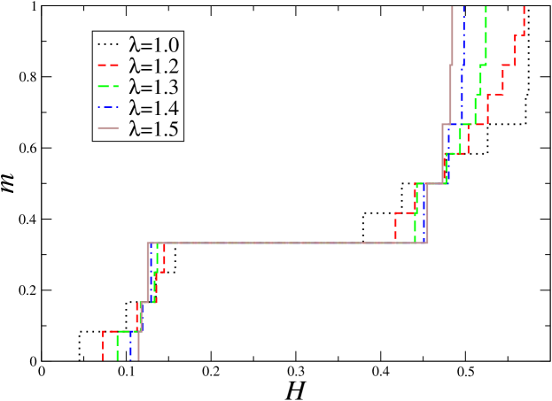
Figure 2: Magnetization curves for $L=8$ calculated by the numerical diagonalization for $\lambda=$1.0, 1.2, 1.3, 1.4 and 1.5.

When $\lambda\sim 1$, the ground-state of the $J_{1}-J_{5}$ chain will be the singlet dimer state which is smoothly connected to the Haldane state of the spin-1 chain.hida In this case, the step of the magnetization curve is $\delta M=1$. On the other hand, the Ising-like anisotropy $\lambda(>1)$ stabilizes the states $|\uparrow\uparrow\rangle$ and $|\downarrow\downarrow\rangle$ at the $J_{1}$ bond (see Fig. 1). As a result each step of the magnetization curve tends to be $\delta M=2$. This two magnon bound state is one of the characters of the spin nematic liquid phase. In fact, some steps with $\delta M=2$ appear in the magnetization curves for $\lambda\geq 1.3$ in Fig. 2. Thus we investigate the possibility of the spin nematic liquid around the magnetization region where the two magnon bound state is realized.

IV 1/3 Magnetization Plateau

At the 1/3 magnetization plateau the Néel order of the $J_{1}-J_{5}$ chain is expected to occur for sufficiently large $\lambda$. The phase transition from the singlet dimer state to the Néel ordered state is of the same universality class of that from the Haldane state to the Néel state of the spin-1 chain. Using the phenomenological renormalization group analysis,nightingale the critical point $\lambda_{\rm c}$ of the quantum phase transition can be estimated. The size-dependent fixed point is determined by the form

$$(L+2)\Delta_{\pi}(L+2,\lambda)=L\Delta_{\pi}(L,\lambda),$$ (4)

where $\Delta_{\pi}(L,\lambda)$ is the gap of the excitation with $k=\pi$ at $m=1/3$. The scaled gap $L\Delta_{\pi}(L,\lambda)$ is plotted versus $\lambda$ for $L=$2, 4, 6 and 8 in Fig. 3(a). The size-dependent fixed point $\lambda_{\rm c}(L+1)$ determined as the cross point of $L\Delta_{\pi}(L,\lambda)$ and $(L+2)\Delta_{\pi}(L+2,\lambda)$ is plotted versus $1/(L+1)^{2}$ in Fig. 3(b). Assuming the size correction is proportional to $1/(L+1)^{2}$, the critical point in the infinite $L$ limit is estimated as $\lambda_{\rm c}=1.342\pm 0.001$.

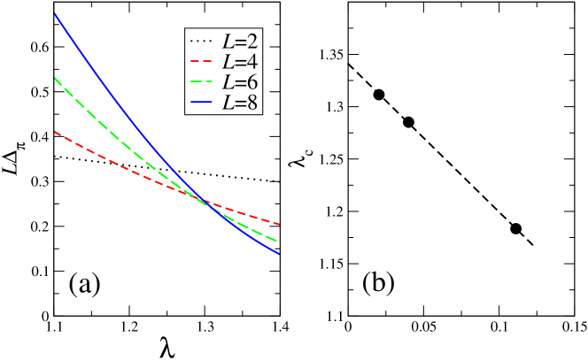
Figure 3: (a) Scaled gaps $L\Delta_{\pi}(L,\lambda)$ are plotted versus $\lambda$ for $L=$2, 4, 6, and 8. (b) Extrapolation of the size-dependent fixed points $\lambda_{c}(L+1)$ to the infinite $L$ limit, assuming the size correction is proportional to $1/(L+1)^{2}$.

V Two Tomonaga-Luttinger liquids

The gapless region in the magnetization process of the quantum spin chain is generally in the Tomonaga-Luttinger liquidhaldane with $\delta M=1$. We call it the conventional Tomonaga-Luttinger liquid (CTLL). The present model is in the CTLL phase around $\lambda=1$. As shown in the section III, the two magnon bound state with $\delta M=2$ can be realized due to the sufficiently large $\lambda$. This phase is called the two-magnon TLL phase. The two-magnon TLL phase by similar mechanism was found in several models.sakai2010 ; sakai2020 ; sakai2021 ; sakai2022 ; sakai2022a ; nakanishi .

The behaviors of several excitation gaps are different between these two TLL phases. The single- and two-magnon excitation gaps are denoted as $\Delta_{1}$ and $\Delta_{2}$. In addition the $2k_{F}(=3/2(1-m)\pi)$ excitation gap of the two magnon bound state is denoted as $\Delta_{2k_{F}}$. The scaled gaps $L\Delta_{1}$, $L\Delta_{2}$ and $L\Delta_{2k_{F}}$ are plotted versus $\lambda$ for $L=$4 and 8 for $m=2/3$. The small (large) $\lambda$ region is in the CTLL (two-magnon TLL) phases. Fig. 4 indicates that $\Delta_{1}$ ($\Delta_{2k_{F}}$) is gapless (gapped) in the CTLL phase, while $\Delta_{1}$ ($\Delta_{2k_{F}}$) is gapped (gapless) in the two-magnon TLL one. In contrast, $\Delta_{2}$ is always gapless. Thus the cross point of $\Delta_{1}$ and $\Delta_{2k_{F}}$ and that of $\Delta_{1}$ and $\Delta_{2}$ are good probes for the estimation of the phase boundary between the CTLL and the two-magnon TLL phases. Here we adopt the former from the viewpoint of the finite-size effect.sakai2022a ; nakanishi

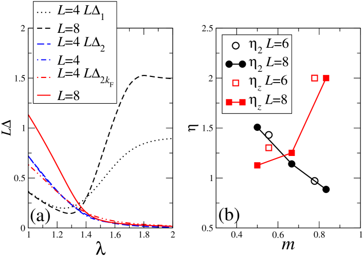
Figure 4: (a) Scaled gaps $L\Delta_{1}$, $L\Delta_{2}$ and $L\Delta_{2k_{F}}$ are plotted versus $\lambda$ for $L=$4 and 8 for $m=2/3$. (b) Exponents $\eta_{2}$ and $\eta_{z}$ estimated for $L=6$ and 8 are plotted versus $m$ for $\lambda=1.5$.

In the two-magnon TLL phase, the quasi-long-range SDW and nematic orders are expected to be realized. They are characterized by the power law decays of the following spin correlation functions

$$\langle S_{1}^{z}S_{3r+1}^{z}\rangle-\langle S_{1}^{z}\rangle^{2} \sim \cos(2k_{\rm F}r)r^{-\eta_{z}}$$ (5)

$$\langle S_{1}^{+}S_{2}^{+}S_{3r+1}^{-}S_{3r+2}^{-}\rangle \sim r^{-\eta_{2}},$$ (6)

where the first equation corresponds to the SDW spin correlation parallel to the external field and the second one corresponds to the nematic spin correlation perpendicular to the external field. The smaller exponent between $\eta_{z}$ and $\eta_{2}$ determines the dominant spin correlation. According to the conformal field theory these exponents can be estimated by the formscardy

$$\eta_{2} = {{E(L,M+2)+E(L,M-2)-2E(L,M)}\over{E_{k_{1}}(L,M)-E(L,M)}},$$ (7)

$$\eta_{z} = 2{{E_{2k_{F}}(L,M)-E(L,M)}\over{E_{k_{1}}(L,M)-E(L,M)}},$$ (8)

for each magnetization $M$, where $k_{1}$ is defined as $k_{1}=L/2\pi$. The exponents $\eta_{2}$ and $\eta_{z}$ estimated for $L=6$ and 8 are plotted versus $m$ for $\lambda=1.5$ in Fig. 4(b). It suggests that the SDW correlation is dominant for small $m$, while the nematic one for large $m$. Neglecting the finite size correction, the cross point of $L=8$ is used as the crossover point between the nematic correlation dominant TLL (NTLL) and the SDW correlation dominant TLL (SDWTLL) phases.

VI Phase Diagram

Finally we obtain the phase diagram with respect to the anisotropy $\lambda$ and the magnetization $m$ in Fig. 5. The phase boundary between the CTLL and the two-magnon TLL phases is estimated as the cross point between $\Delta_{1}$ and $\Delta_{2k_{F}}$ for $L=6$ and 8 (solid circles and squares, respectively). The crossover line is determined by $\eta_{2}=\eta_{z}$ (red diamonds). At the 1/3 magnetization plateau the boundary of the Néel ordered phase is determined by the phenomenological renormalization (up triangle). This boundary is expected to be connected to the one between the CTLL and two-magnon TLL phases. The boundary at $m=1$ can be easily determined by $\Delta_{1}=\Delta_{2}$. The magnetization process at $0<m<1/3$ is also expected to be in the TLL phase. However, whether some multi-magnon TLL phases possibly appear or not is still an unsolved problem.

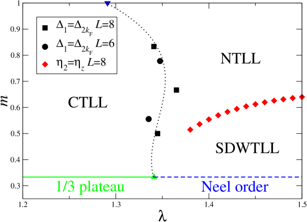
Figure 5: Phase diagram with respect to the anisotropy $\lambda$ and the magnetization $m$.

VII Summary

The $S=1/2$ distorted diamond spin chain with the anisotropic ferromagnetic interaction is investigated using the numerical diagonalization. As a result it is found that as the nematic correlation dominant TLL phase can appear for a sufficiently large anisotropy, as well as the SDW correlation dominant TLL phase. The phase diagram with respect to the anisotropy and the magnetization is also presented.

Data Availability

The data that support the findings of this study are available from the corresponding author upon reasonable request.

References

- (1) A. F. Andreev and A. Grishchuk, Sov. Phys. JETP 60, 267 (1984).
- (2) H. H. Chen and P. M. Levy, Phys. Rev. Lett. 27, 1383 (1971).
- (3) J. Sudan, A. Lüscher, and A. M. Läuchli, Phys. Rev. 80, 140402(R) (2009).
- (4) T. Hikihara, L. Kecke, T. Momoi and A. Furusaki, Phys. Rev. B 78, 144404 (2008).
- (5) T. Sakai, T. Tonegawa, and K. Okamoto, Phys. Status Solidi B 247, 583 (2010).
- (6) T. Sakai and K. Okamoto, JPS Conf. Proc. 30, 011083 (2020).
- (7) T. Sakai, AIP Advances 11, 015306 (2021).
- (8) T. Sakai, H. Nakano, R. Furuchi and K. Okamoto, J. Phys.: Conf. Ser. 2164, 012030 (2022).
- (9) T. Sakai, R. Nakanishi, T. Yamada, R. Furuchi, H. Nakano, H. Kaneyasu, K. Okamoto, and T. Tonegawa, Phys. Rev. B 106, 064433 (2022).
- (10) R. Nakanishi, T. Yamada, R. Furuchi, H. Nakano, H. Kaneyasu, K. Okamoto, T. Tonegawa, and T. Sakai, to be published in JPS Conf. Proc.: arXiv:2209.09740.
- (11) H. Kikuchi, Y. Fujii, M. Chiba, S. Mitsudo, T. Idehara, T. Tonegawa, K. Okamoto, T. Sakai, T. Kuwai, and H. Ohta, Phys. Rev. Lett. 94, 227201 (2005).
- (12) K. Okamoto T. Tonegawa Y. Takahashi, and M. Kaburagi, J. Phys.: Condens. Matter, 11, 10485 (1999).
- (13) K. Okamoto, T. Tonegawa, and M. Kaburagi, J. Phys.: Condens. Matter, 15, 5979 (2003).
- (14) M. Fujihala, H. Koorikawa, S. Mitsuda, M. Hagihala, H. Morodomi, T. Kawae, A. Mitsudo, and K. Kindo, J. Phys. Soc. Jpn. 84, 073702 (2015).
- (15) K. Morita, M. Fujihala, H. Koorikawa, T. Sugimoto, S. Sota, S. Mitsuda and T. Tohyama, Phys. Rev. B 95, 184412 (2017).
- (16) M. Fujihala, H. Koorikawa1, S. Mitsuda, K. Morita, T. Tohyama, K. Tomiyasu, A. Koda, H. Okabe, S. Itoh, T. Yokoo, S. Ibuka, M. Tadokoro, M. Itoh, H. Sagayama, R. Kumai and Y. Murakami, Sci. Rep. 7, 16785 (2017).
- (17) K. Hida, Phys. Rev. B 45, 2207 (1992).
- (18) P. Nightingale, J. Appl. Phys. 53, 7927 (1982).
- (19) F. D. M. Haldane, J. Phsy. C 14, 2585 (1981).
- (20) J. L. Cardy, J. Phys. A: Math. Gen. 17, L385 (1984).