Generating EPR-pairs from an -party resource state
Abstract
Motivated by quantum network applications over classical channels, we initiate the study of -party resource states from which LOCC protocols can create EPR-pairs between any disjoint pairs of parties. We give constructions of such states where is not too far from the optimal while the individual parties need to hold only a constant number of qubits. In the special case when each party holds only one qubit, we describe a family of -qubit states with proportional to based on Reed-Muller codes, as well as small numerically found examples for and . We also prove some lower bounds, for example showing that if then the parties must have at least qubits each.
1 Introduction
1.1 Generating EPR-pairs from a resource state
Quantum communication networks combine several quantum computers to enable them to solve interesting tasks from cryptography, communication complexity, distributed computing etc. Building a large-scale quantum communication network is a daunting task that will take many years, but networks with a few small quantum computers are under construction and may start to appear in the next few years [WEH18].
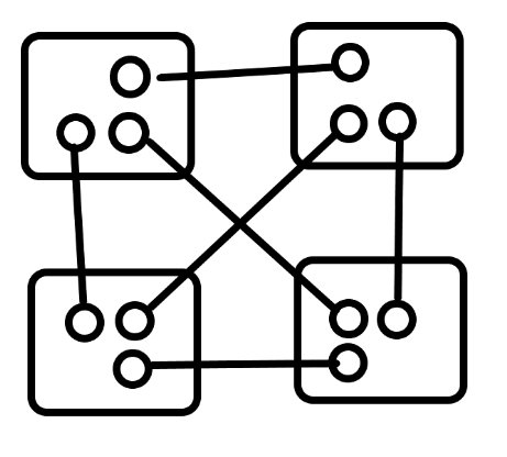
These networks are either based on channels that physically communicate quantum states, or rely on classical communication in tandem with shared entanglement, or a combination of both. Communication over classical channels cannot increase entanglement, so in the absence of quantum channels we have to rely on prior entangled states. For example, if two parties share an EPR-pair, , then one party can transmit (“teleport”) a qubit to the other via two classical bits of communication, consuming the EPR-pair in the process [BBC+93]. If we want to enable many qubits to be sent in this way, then we could start with an entangled state where each pair among the parties shares its own EPR-pair. This would allow any pair to exchange a qubit, but would require us to start with a rather large initial entangled state of EPR-pairs, and each of the parties would need to hold qubits (see Figure 1 for ).
Now suppose that we know in advance that only some pairs out of the parties will be required to exchange a qubit, but we do not know in advance what those pairs are. In this paper we study what initial -party resource states are sufficient or necessary to achieve this task. Note that an EPR-pair between two parties allows them to exchange a qubit in either direction via local operations and classical communication (LOCC), and conversely the ability to exchange a qubit between two parties allows them to share an EPR-pair (one party locally creates the EPR-pair and sends one of its qubits to the other party). This shows that the ability to exchange qubits between any disjoint pairs of parties is essentially equivalent to the ability to establish EPR-pairs between any disjoint pairs. We focus on the latter task in this paper.
We call an -party state -pairable if for every disjoint pairs of parties, there exists an LOCC protocol that starts with and ends up with a state where each of those pairs of parties shares an EPR-pair. The local quantum operations and the classical communication are free, but we do care about the number of qubits per party in : the fewer the better. The same resource state has to work for every possible -pairing, so it is fixed before the pairing task is given. For example, the -qubit GHZ-state
is 1-pairable: in order to obtain an EPR-pair between two parties Alice and Bob, the other parties can measure their qubit in the Hadamard basis and communicate the classical measurement outcomes to Alice and Bob, who convert their remaining 2-qubit state into an EPR-pair if one of them (say Alice) does a -gate conditioned on the parity of the bits they received.
The GHZ-example has the minimal possible 1 qubit per party, but unfortunately is only 1 there. We are interested in resource states that are -pairable for larger . We give both upper and lower bounds for -pairability, considering both the situation where we allow qubits per party (but not too many), and the situation where we insist that each of the parties has only the minimal qubits.
1.2 Our results 1: constructions of -pairable resource states
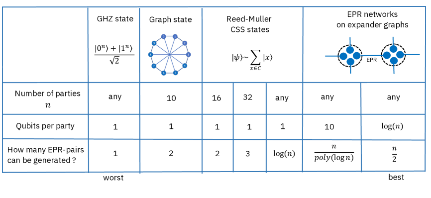
In Section 2 we first study -pairable resource states where each of the parties is allowed to have qubits (hence will have qubits in total). We show that we can make as large as while each party holds only 10 qubits. Roughly, the idea is to take a special kind of -vertex expander graphs that guarantee existence of edge-disjoint paths for any disjoint pairs, let each edge in the graph correspond to an EPR-pair, and create the desired EPR-pairs via entanglement-swapping along the edge-disjoint paths. If we allow qubits per party instead of , then we can construct -pairable resource states with , meaning that from our fixed resource state we can create EPR-pairs across any perfect matching of the parties into disjoint pairs.111Note that if we allow one party to hold many more qubits than the others, then we could use a star graph, where the central party shares an EPR-pair with each of the other parties, and uses entanglement-swapping (see the proof of Lemma 1) to link up the pairs as desired. This -qubit state is -pairable for the maximal , and parties hold the minimal 1 qubit. However, the central party holds qubits and has to do all the work in obtaining the -pairing. In the spirit of the small quantum networks of small quantum computers that we’ll have in the near and medium-term future, we prefer constructions where none of the parties needs to hold many qubits. This result essentially requires only classical off-the-shelf routing arguments.
Since qubits are expensive, especially when lots of error-correction is needed to protect them, we also look at what is possible when each party holds only 1 qubit, which is of course the bare minimum. In this case, we construct -party (which in this case is the same as -qubit) resource states for the case for arbitrary (this corresponds to the GHZ-state). For it is not clear that pairability is a property monotone in . What we have is that -pairable states exist for for and higher powers of 2 (we also give numerical evidence for the existence of a 2-pairable state on qubits); for for and higher powers of 2; and for arbitrary for and higher powers of 2. These resource states will be superpositions over the codewords in a Reed-Muller code, and we use the stabilizer formalism to design LOCC protocols for obtaining the desired EPR-pairs from the resource state. Our construction is efficient in the sense that all steps in the LOCC protocol can be computed in time . To prove correctness of the protocol we reduce the problem of EPR-pair generation to a version of the polynomial regression problem: constructing a multi-variate -valued polynomial of fixed degree that takes prescribed values at a given set of points. One of our main technical contributions is developing tools for solving a particular family of such polynomial regression problems.
1.3 Our results 2: obstructions
Next we look at obstructions, namely lower bounds on the achievable tradeoff between , , and . First consider the case where we can pair up any disjoint pairs. An ideal resource state would allow us to do this (i.e., be -pairable) with only qubits per party. As mentioned above, we have shown that -pairability with only 1 qubit per party is indeed achievable if , but in Section 4 we show it is not achievable if : in that case qubits per party are needed. The proof is by an intricate dimension-counting argument, which gives upper and lower bounds on the dimension of the space of states that can be reached (with non-zero probability) by LOCC protocols on a fixed -qubit resource state . In Section 5 we extend this approach to the case of partial pairings, so where , showing in this more general case. In particular, if then can be at most , so achieving something close to complete pairability (i.e., ) requires a super-constant number of qubits per party. Up to the power of the polylog, this matches our construction of -pairable states with and qubits per party (Section 1.2).
1.4 Related work
To the best of our knowledge, the problem of what resource states allow LOCC protocols to construct EPR-pairs between any pairs of parties has not been studied before. However, we are aware of a number of related works, which we will briefly discuss here.222We won’t go over the literature on quantum network coding (which assumes the ability to send qubits over specific edges) nor the massive experimental physics literature on preparation of entangled states on actual noisy hardware such as optical links and repeaters. These works can be organized into two categories.
Entanglement routing assisted by quantum communication.
Here some parties are allowed to exchange qubits in addition to performing LOCC on the initial resource state.
Schoute et al. [SMI+16] consider quantum networks where parties can create EPR-pairs with their immediate neighbors and then use entanglement-swapping combined with efficient routing algorithms to create desired long-distance entanglement. This differs from our approach in allowing the ability to create new EPR-pairs when needed (which requires quantum communication), while we allow only LOCC starting from one fixed entangled resource state.
Hahn, Pappa, and Eisert [HPE19] also study a quite similar problem to ours, but starting from a network where some parties are linked via a quantum channel, while some other parties are not (directly) linked at all. In addition to efficiently generating EPR-pairs they also study generating GHZ-states between specified parties.
Pant et al. [PKT+19] study how a network whose nodes are connected via lossy optical links and have limited quantum processing capabilities, can obtain EPR-pairs simultaneously between many pairs of nodes; their limitations per node are analogous to our goal of having only few qubits per party, but they allow quantum communication while we allow only classical communication.
Restricted variants of -pairability.
Here the parties are only allowed to perform LOCC on the initial resource state. The parties may be able to generate EPR pairs for some but not all choices of such pairs.
Miguel-Ramiro, Pirker, and Dür [MPD23] consider resource states interpolating between the two extreme cases discussed in our introduction: the GHZ state shared among parties and EPR states shared between each pair of parties. This work proposed clustering and merging algorithms that produce resource states with the desired functionality. However, these methods do not appear to provide -pairable resource states with few qubits per party.
Du, Shang, and Liu [DSL17] study a problem similar to ours but starting from resource states that consist only of pre-shared EPR-pairs between adjacent parties in a given network. Like us, they use entanglement-swapping to create EPR-pairs between distant parties.
Contreras-Tejada, Palazuelos, and de Vicente [CPdV22] gave similar constructions as we gave in Section 2 (with EPR-pairs on the edges of an -vertex graph), but focus primarily on the question for what type of graphs the long-range entanglement survives constant amounts of noise on the edges.
Illiano et al. [IVK+22] study 1-pairable states with the additional property that the identity of the one pair that ends up sharing an EPR-pair remains unknown to the other parties (in fact one can get this easily from the -party GHZ-state if the other parties broadcast their measurement outcomes to everyone rather than sending it only to the two parties that want an EPR-pair).
Meignant, Markham, and Grosshans [MMG19] and Fischer and Townsley [FT21] studied what is roughly a partial “dual” of our problem: how many EPR-pairs between which parties of a given -party network are necessary and sufficient to generate a classically given -party graph state?
Dahlberg, Helsen, and Wehner [DHW20] show that it is NP-complete to decide whether a classically given -party stabilizer state can be transformed into a set of EPR-pairs on specific qubits using only single-qubit Clifford operations, single-qubit Pauli measurements and classical communication (such protocols are more restricted than the LOCC we allow in our paper). They also give some algorithms to do the transformation in some special cases [DHW18].
2 Constructions with multiple qubits per party
In this section we combine classical network routing strategies and the standard entanglement swapping protocol to construct -party -pairable resource states with nearly linear in , such that each party holds at most qubits. Increasing the number of qubits per party from a constant to yields maximally pairable resource states with .
Suppose is a graph with vertices . Vertex represents the -th party. We place two qubits at every edge such that in total there are qubits. Define an -party resource state
where is an EPR-pair located on an edge . The state is shared among parties such that the two qubits located on an edge are assigned to the parties and who share the EPR-pair . Thus each party shares one EPR-pair with each of its neighbors. Accordingly, each party holds at most qubits, where is the maximum vertex degree of .
Lemma 1.
The resource state is -pairable if for any choice of disjoint pairs of vertices in the graph , there exist edge-disjoint paths such that the path connects vertices .
Proof.
Suppose Charlie shares an EPR-pair with Alice and another EPR-pair with Bob. The following well-known entanglement-swapping protocol uses LOCC to create an EPR-pair between Alice and Bob. First, Charlie measures the parity of his two qubits in the standard basis , sends the 1-bit measurement outcome to Bob, and conditioned on it he applies a (bitflip) on his second qubit and Bob applies a to his qubit. This results in a 4-qubit GHZ-state . Now Charlie measures each of his two qubits in the Hadamard basis , sends the parity of the two outcomes to Bob, who conditioned on that bit applies a (phaseflip) to his qubit. It may be verified that now Alice and Bob share an EPR-pair.
The creation of the EPR-pairs using the edge-disjoint paths is now fairly straightforward: the parties on the path from to use the EPR-pairs with their neighbors on the path to create an EPR-pair between and via entanglement-swapping. Because the paths are edge-disjoint, no edge (=EPR-pair) is used more than once. ∎
Below it will be convenient to relax the edge-disjointness condition in Lemma 1 and consider pairability by nearly edge-disjoint paths. More precisely, suppose is an integer. Consider a resource state such that each copy of is shared among parties as specified above. Then each party holds at most qubits, where is the maximum vertex degree of . Each party shares EPR-pairs with each of its neighbors. An immediate corollary of Lemma 1 is the following.
Corollary 2.
The resource state is -pairable if for any choice of disjoint pairs of vertices in the graph , there exist paths such that the path connects vertices and each edge of belongs to at most paths.
To keep the number of qubits per party small, we would like the graph to have a small vertex degree and, at the same time, allow vertex pairability by (nearly) edge-disjoint paths for any choice of disjoint vertex pairs. We would like to maximize the pairability parameter while keeping the vertex degree as small as possible. Luckily, the problem of constructing such graphs has been already studied due to its importance for classical communication networks. A graph is said to have edge expansion if for any subset of vertices with , the number of edges that have exactly one endpoint in is at least . We shall use the following fact.
Fact 1 (Broder, Frieze, Upfal [BFU94]).
For any constants and there exists a constant such that the following is true. Suppose is an -vertex -regular graph with edge expansion at least . Then for any choice of disjoint vertex pairs in there exists a family of paths connecting the chosen pairs of vertices such that every edge of belongs to at most two paths. These paths can be found in time .
It is known [Bol88] that -regular graphs with edge expansion exist for any constant and all large enough . Thus Corollary 2 and Fact 1 imply that for all large enough there exist -pairable resource states with and at most 10 qubits per party.
Let us say that a graph is path-pairable if the number of vertices is even and the condition of Lemma 1 holds for . We shall need the following fact stated as Corollary 2 in [GMM17].
Fact 2 (Győri, Mezei, Mészáros [GMM17]).
For any integer there exists a -regular -vertex path-pairable graph with and .
Combining Lemma 1 and Fact 2 we infer that qubits per party suffices for complete pairings, in contrast with the naive resource state where every one of the pairs shares an EPR-pair and hence each party holds qubits.
Corollary 3.
There exists a family of -party -pairable resource states with qubits per party.
3 Constructions that use only one qubit per party
In this section we study -pairability of -party quantum states under the most stringent restriction: each party holds only one qubit (obviously, -pairability with is impossible if some party has no qubits). This problem is well-motivated since qubits, especially error-corrected logical qubits, built on top of multiple physical qubits, are expensive and we would prefer to have -party -pairable resource states with as few qubits per party as possible.
We have already seen that the -qubit GHZ-state shared by parties is -pairable. Naively, one might think that the GHZ-example is already best-possible and is as far as one can get with one qubit per party. Surprisingly, this naive intuition turns out to be wrong. Here we give examples of -pairable states with one qubit per party for an arbitrary . We choose the resource state as the uniform superposition of codewords of a suitable linear code of codelength . The GHZ-example with is the special case with the repetition code .
To achieve -pairability for we choose as the Reed-Muller code with a suitable parameter , see below for details.333We follow the standard notation for the parameter of Reed-Muller codes. It should not be confused with the number of qubits per party, which equals 1 throughout this section. The LOCC protocol converting to the desired EPR-pairs can be described by a pair of disjoint subsets such that all qubits contained in and are measured in the standard basis and the Hadamard basis respectively. The protocol creates EPR-pairs on qubits contained in the complement . Here . Finally, a Pauli correction or is applied to each EPR qubit . The correction depends on the measurement outcomes and requires classical communication from parties in to parties .
Our construction is efficient in the sense that the subsets of qubits and can be computed in time for any given choice of EPR qubits. Furthermore, the initial resource state can be prepared by a quantum circuit of size . While describing the subsets and is relatively simple, proving that the resulting LOCC protocol indeed generates the desired EPR-pairs is considerably more complicated in the case , as compared with the GHZ-example for . For resource states based on Reed-Muller codes , we will see below that the proof can be reduced to solving a polynomial regression problem: constructing a polynomial of degree whose values are fixed at a certain subset of points . The number of qubits used by our construction is given by , , and for (note that the number of qubits is the same as the number of parties throughout this section). While this scaling may be far from optimal, the main value of our result is demonstrating that -pairability with an arbitrary is possible in principle even in the most restrictive setting with one qubit per party. To the best of our knowledge, this was not known prior to our work. We leave as an open question whether -pairable states based on Reed-Muller codes can achieve a more favorable scaling or even the scaling that can be achieved if we allow 10 qubits per party instead of 1 (end of Section 2). Such an improvement may require consideration of more general LOCC protocols that use all three types of Pauli measurements, in the bases.
Finally, we describe a numerically-found example of a -qubit -pairable state with one qubit per party; this is more efficient than the 16-qubit -pairable state from the above results. This example is based on a stabilizer-type resource state and an LOCC protocol with Pauli measurements. We also show that no stabilizer state with qubits is -pairable using only Pauli measurements. In that sense our -qubit example is optimal.
The rest of this section is organized as follows. We introduce CSS-type resource states and give sufficient conditions for -pairability of such states in Section 3.1. Reed-Muller codes and their basic properties are described in Section 3.2. We define resource states based on Reed-Muller codes and describe our LOCC protocol for generating EPR-pairs in Section 3.3. A proof of -pairability for , and for an arbitrary is given in Sections 3.4, 3.5, and 3.6 respectively. Finally, we describe the -qubit -pairable example in Section 3.7.
3.1 Pairability of CSS stabilizer states
To describe our construction we need more notation. Let be the -dimensional vector space over . Given a vector and a bit index , let be the -th bit of . We write for the dot product of vectors . Unless stated otherwise, addition of binary vectors and the dot product are computed modulo two. The weight of a vector is the number of bits such that . A linear code of length is simply a linear subspace . Vectors are called codewords. The code is said to have distance if any nonzero codeword has weight at least . The dual code of , denoted , is the subspace of vectors such that for all . An affine subspace of dimension is a set of vectors , where is a linear subspace of dimension and is some fixed vector.
Suppose our -qubit resource state has the form
| (1) |
where is a linear code. Such states are known as Calderbank-Shor-Steane (CSS) stabilizer states [CS96, Ste96, CRSS98]. It is well-known that the state can be prepared by a quantum circuit of size for any linear code , see for instance [AG04]. We begin by deriving a sufficient condition under which a CSS stabilizer state is -pairable. Below we assume that each of the parties holds only one qubit.
Lemma 4 (Pairability of CSS stabilizer states).
Suppose is a linear code. Suppose for any set of disjoint pairs of qubits there exists a partition of the qubits into three disjoint subsets
| (2) |
such that and the following conditions hold for all :
- CSS1:
-
such that and for all :
- CSS2:
-
such that and for all :
Then the -qubit state is -pairable.
Here and below we use shorthand set union notation whenever and are disjoint sets. The desired EPR-pairs can be generated in three steps. First, each qubit is measured in the standard basis and each qubit is measured in the Hadamard basis . Next, each party broadcasts their binary measurement outcome to . Finally, a Pauli correction is applied to each qubit ; this may depend on the measurement outcomes.
Proof of Lemma 4.
We assume some familiarity with the stabilizer formalism [CS96, Got98, NC02]. Let and be single-qubit Pauli operators acting on the -th qubit tensored with the identity on all other qubits. The resource state has Pauli stabilizers444Note that for any . Here the third equality uses the fact that is a linear code, i.e., a subspace. Furthermore, since for any and .
and
Thus we have . Suppose and obey conditions CSS1, CSS2 for some pair . Let be the measurement outcome on a qubit . Condition CSS1 implies that the stabilizer commutes with Pauli operators on qubits , which are measured in the standard basis. Thus and are stabilizers of the final state after the measurement. We infer that the final state is stabilized by
Here the second equality follows from CSS1. Likewise, CSS2 implies that the stabilizer commutes with Pauli operators on qubits , which are measured in the Hadamard basis. Thus and are stabilizers of the final state. We infer that the final state is stabilized by
Here the second equality follows from CSS2. This is only possible if the final state contains an EPR-pair on the qubits , up to a Pauli correction and/or . The correction can be applied via LOCC if each party broadcasts their measurement outcome to all parties . ∎
3.2 Reed-Muller codes
First, let us record the definition and some basic properties of Reed-Muller codes. Let be an integer. A Boolean function can be considered as a binary vector of length which lists the function values for all inputs in some fixed (say, the lexicographic) order. For example, if and then we can consider as a length- binary vector
Reed-Muller code has length and its codewords are the -bit vectors associated with -variate degree- polynomials . One can choose generators of as a set of monomials where runs over all subsets of of size at most . The monomial associated with the empty set is the constant-1 function. For example, is the repetition code of length since there are only two degree- polynomials: and . We shall use the following facts.
Fact 3 (Code parameters).
The Reed-Muller code has dimension
and distance .
Fact 4 (Dual code).
Suppose . Then .
Fact 5 (Affine invariance).
Suppose is an invertible matrix, and is a vector. If is a degree- polynomial, then the function is also a degree- polynomial. The map is a bijection of the set of all -variate degree- polynomials.
For the proof of Facts 3, 4, 5, see e.g. Chapter 13 of [MS77]. As a consequence of Fact 5, the resource state with is invariant under a permutation of the qubits defined as , where for all . Here is any invertible affine map. In other words, . This generalizes the symmetry of the -qubit GHZ-state which is invariant under any permutation of the qubits.
Recall that minimum-weight codewords of a linear code are non-zero codewords whose weight equals the code distance.
Fact 6 (Codewords from affine subspaces).
A vector is a minimum-weight codeword of if and only if the support of is an -dimensional affine subspace of .
For the proof see, e.g., Proposition 2 and Corollary 4 in [AJ92]. We shall see that verification of conditions CSS1 and CSS2 of Lemma 4 with can be reduced to (multiple instances of) the following problem.
Problem 1 (Polynomial regression).
Find a degree- polynomial that satisfies a system of equations
| (3) |
where are distinct points and .
Lemma 5.
The polynomial regression problem has a solution if at least one of the following conditions is satisfied: (1) , or (2) and .
Here the sum is evaluated modulo two.
Proof.
by Fact 4. The code has distance , see Fact 3, and thus every columns of its parity check matrix are linearly independent. The parity check matrix of is the generator matrix of its dual, , so the above implies that if , then the rank of the matrix formed by the columns of with indices from is , so is in the span of the rows of .
If , then the rank of is either or . If , we proceed as above. If , the only linear combination of the columns of that gives the zero-vector, is the sum of all columns of , and a vector can be generated from the rows of if and only if . ∎
3.3 Resource state and LOCC protocol
Our candidate -pairable state is a CSS stabilizer state with
| (4) |
and a suitable parameter . To describe the subsets of qubits satisfying conditions CSS1 and CSS2 of Lemma 4, we need one extra piece of notation.
Definition 1.
Suppose is a non-empty subset. An affine subspace spanned by , denoted , is defined as
| (5) |
Thus contains all vectors that can be written as a sum of an odd number of vectors from . For example, , , and . Note that , where is the dimension of .
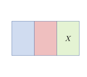
Let be the number of qubits. Suppose our goal is to generate EPR-pairs on pairs of qubits . Define a subset of “EPR qubits”
and a family of affine subspaces such that
| (6) |
where are vectors that will be appropriately defined in Sections 3.4, 3.5, 3.6. The -vectors may depend on the ’s and ’s. The set of EPR qubits is obviously contained in the union of . We choose the subsets of qubits and in Lemma 4 as
| (7) |
The subsets are pairwise disjoint and . We illustrate the relationships between these sets in Figure 3. In the GHZ-example one has and . In this case and , that is, the LOCC protocol requires only measurements in the Hadamard basis. In the rest of this section we prove that the vectors in Eq. (6) can always be chosen such that the subsets and satisfy conditions CSS1 and CSS2 of Lemma 4.
3.4 -pairability
We now need to show how to choose . We begin with the simple case .
Lemma 6.
Proof.
Note that a vector as above exists since and for . Specializing Eq. (6) to the case and one gets
| (8) |
The assumption that implies that the are 2-dimensional affine subspaces, and in particular, (). We claim that
| (9) |
Indeed, by definition, . Suppose . Since all EPR qubits are distinct, the inclusion is only possible if or . In both cases , which contradicts the choice of . Thus . Applying the same arguments to proves Eq. (9).
Let us first check condition CSS2 with (the same argument applies to ). Choose
Since is a -dimensional affine subspace, Fact 6 implies that . We have since . From Eq. (9) one gets . Thus for all , as claimed. This proves condition CSS2.
Let us check condition CSS1 with (the same argument applies to ). We can invoke Lemma 5 (polynomial regression) with and to show that there exists a degree- polynomial such that
| (10) |
We can use condition (2) of Lemma 5 since . By definition, is a codeword of and . We need to check that for all . By definition,
We already know that by Eq. (10). Since is a degree- polynomial, one has
Likewise, . If , then we are done. Suppose . Since there is an affine subspace with co-dimension one, which contains , but . Let be the linear function that is on and 1 on . Let . Then on takes the same values as , but , and we apply the above argument for instead of . This proves CSS1. ∎
3.5 -pairability
In the case we choose and . The resource state requires qubits. We checked conditions CSS1 and CSS2 of Lemma 4 numerically using exhaustive search over all tuples of EPR qubits and all choices of vectors in the definition of subsets and . It was observed that for any tuple of EPR qubits, there exists at least one choice of the -vectors such that and obey conditions CSS1 and CSS2. The search space was pruned by exploiting the affine invariance of Reed-Muller codes, see Fact 5. Namely, choose any invertible affine map such that and . Fact 5 implies that a permutation of the qubits described by is an automorphism of . Thus this permutation of qubits leaves the resource state invariant and we can assume w.l.o.g. that and . We also pruned the search over the -vectors by imposing a constraint which is analogous to the constraint used for . The remaining search over took less than one hour on a laptop computer. Note that the affine invariance of Reed-Muller codes also implies that is -pairable for all since we can always apply an affine map as above such that and has nonzeros only on the first bits. We note that the choice of parameters , is minimal for -pairability of resource states , as follows from a simple code distance argument.555-pairability of the CSS resource state requires both codes and to have minimum distance at least since otherwise a stabilizer of may have support on a subset of the EPR qubits and anti-commute with some stabilizer of the target EPR-pairs. In particular, -pairability requires and to have distance at least . Reed-Muller codes do not have this property for and , see Facts 3, 5. Meanwhile, the code is self-dual and has distance .
3.6 -pairability for an arbitrary (and sufficiently large )
In this section we prove that the resource state is -pairable for any and (note that the number of parties can be any ). First let us exploit the affine invariance of Reed-Muller codes (Fact 5) to convert the set of EPR qubits into a certain standard form. Choose a linear invertible map such that and have zeros on the first bits for all (recall that we label the qubits by -bit strings). This is always possible for . Since the state is invariant under the permutation of the qubit-labels associated with , we can replace by and . Accordingly, from now on we assume that and have zeros on the first bits. The linear map can be computed in time using Gaussian elimination. In addition, we can assume that
| (11) |
Indeed, to see this, suppose is a vector whose first bits are zero, and none of the vectors or belongs to the set . Using the affine invariance of Reed-Muller codes one can replace and by and . The new vectors obey the extra condition Eq. (11). The number of bad s (s we should not pick) is at most
(upper bounding the number of all possible differences between the two sets). The number of s we can pick from (all those vectors starting with 0s) is at least . Now (which holds for all ) gives the claimed property. Hence, from now on we assume Eq. (11).
We choose vectors in Eq. (6) as the basis vectors of such that the -th bit of is 1 and all other bits of are 0,
| (12) |
Thus the -vectors are supported on the first bits while all - and -vectors are supported only on the last bits. Next we use Eqs. (6,7) to define the subsets of qubits to be measured in the Hadamard () and in the standard () basis, respectively. For convenience, we restate the definitions of , , and below.
It remains to prove that and satisfy conditions CSS1, CSS2 of Lemma 4 with
Below we shall use the following property.
Proposition 7.
The affine subspace is -dimensional and obeys
| (13) |
Proof.
We have since all -vectors are linearly independent and have zeros on the last bits, while , have zeros on the first bits and . Thus is -dimensional.
Let us check Eq. (13). By definition, contains both and . Suppose and . Then is an odd linear combination of vectors . Recall that the last bits of all -vectors are zero and the first bits of all - and -vectors are zero. Thus must be an odd linear combination of vectors and only. This is only possible if or . However, we assumed that all EPR qubits are distinct. Thus . The same argument shows that . ∎
First let us check condition CSS2 with (the same argument works for any ). Choose a function as
Since is a -dimensional affine subspace, Fact 6 implies that . We have since . From Eq. (13) one gets . Thus for all , as claimed. This proves condition CSS2.
Checking condition CSS1 requires more technical work, and we strongly encourage the reader to first study the proof of a quite general special case in Appendix A, which is much simpler.
As before, we can focus on the case (the same argument works for any ). Then condition CSS1 is equivalent to the existence of a degree- polynomial such that
| (14) |
Any degree- polynomial can be written as
| (15) |
where is some polynomial of degree that depends only on the variables . It remains to choose the polynomials with . We shall use induction on starting with . At each induction step we shall use polynomial regression (Lemma 5) to argue that the desired polynomial exists (there is no need to construct explicitly). Given , define the following set of -bit strings
| (16) |
Proposition 8.
Proof.
CSS1 requires that takes given values on , namely , and must be zero on the rest of . When we plug these input values into Eq. (15), it is a straightforward calculation to see that Eq. (17) exactly says that if and only if , and Eq. (18) exactly says that for all . More precisely, Eq. (18) for some and expresses exactly for , where is the characteristic vector of . Eq. (16) was engineered so that the above ranges over all of . ∎
In the rest of the section we concentrate our efforts on finding a family of polynomials that satisfy Proposition 8. Below we focus on the case when is even. The analysis for odd requires only a few minor modifications, as detailed in Appendix B.
For fixed and we recursively (in the increasing size of ) construct , and inductively show that has the desired properties. To enable induction, we supplement Eqs. (17,18) with a few extra conditions on the polynomials . Let be an integer. We will say that a family of polynomials labeled by subsets with is valid if all conditions stated below are satisfied for :
-
I1:
depends only on the variables
-
I2:
has degree
-
I3:
and for
-
I4:
for every non-empty set and every
-
I5:
if is odd and
-
I6:
if and
-
I7:
if and
Here (I1,I3,I4) are the conditions stated in Proposition 8 and (I2) ensures that a polynomial constructed from the family according to Eq. (15) has degree . Thus (I1,I2,I3,I4) alone imply CSS1. We shall use induction on to prove that a valid family of polynomials exists for all . The extra conditions (I5,I6,I7) facilitate analysis of the induction step.
The base case of the induction is . Then a valid family is a single polynomial . Condition (I2) demands that has degree . Conditions (I4) and (I5) can be skipped for . Condition (I7) follows trivially from (I3). It remains to check (I3,I6) Note that conditions (I3) and (I6) with are imposed at disjoint set of points, see Eq. (11). Thus (I3) and (I6) are consistent. We fix the value of at points in (I3) if , and at points in (I3,I6) if . We can show that the desired polynomial exists using Lemma 5. Below we always apply the lemma to polynomials satisfying condition (I1). This is justified since the first bits of all vectors and are zero. If then we have . Thus we can use part (2) of Lemma 5. The extra condition of the lemma is satisfied since (I3) fixes the value of to at an even number of points. If then we have and thus we can use part (1) of Lemma 5.
We shall now prove the induction step. Suppose we have already constructed a valid family of polynomials with . Consider a subset with such that . The case will be considered afterwards.
Suppose is odd. Since is even and , this is only possible if . We set to satisfy (I5). Then conditions (I2), (I6), (I7) are satisfied automatically. Condition (I3) can be skipped since . Condition (I4) with demands that for any . Since is odd, is the set of points and with . Each term with odd vanishes due to (I5). Each term with even vanishes for due to (I6) since . Thus choosing satisfies (I4).
Suppose is even. Condition (I2) demands that has degree . Conditions (I3), (I5) can be skipped since is even and . We claim that (I7) follows from (I4). Indeed, we have iff or with . We have due to (I4). If is odd then due to (I5) since . If is even then . Thus since (I7) holds for . This implies for any , as claimed in (I7). It remains to check (I4,I6). We fix the value of at points in (I4) if . We fix the value of at points in (I4,I6) if . Consider first the case . Then since and are even. Thus and . We can use part (2) of Lemma 5 to construct . The extra condition of the lemma is equivalent to
| (19) |
Each term with odd vanishes due to (I5) since . Each term with even obeys for since obeys (I7). Thus we have for any which implies Eq. (19). Thus the desired polynomial exists by part (2) of Lemma 5, that is, we have checked (I4) in the case . Condition (I6) can be skipped in this case. In the remaining case, , we can use part (1) of Lemma 5 since for . Thus conditions (I4,I6) are satisfied.
It remains to prove the induction step for . Suppose we have already constructed a valid family of polynomials with . Consider a subset with . Since we assumed that is even, is odd. Condition (I2) demands that has degree , that is, is a constant function. We can skip conditions (I3,I5,I6,I7) since none of them applies if . It remains to check (I4). Note that for some such that . Condition (I4) fixes the value of at and at . Since we want to be a constant function, it suffices to check that the desired values and are the same. Substituting the desired values from (I4), we have to check that
| (20) |
The sum contains terms with . All terms with odd must have since is even. Such terms vanish due to (I5). All terms with even vanish due to (I6). Thus we can restrict the sum Eq. (20) to terms with . However, is a degree-1 polynomial if due to (I2). Thus and Eq. (20) is equivalent to
| (21) |
Since obeys (I7), we have , which implies Eq. (21). We have now verified (I4). This completes the proof of the induction step.
Accordingly, having shown that both conditions CSS1 and CSS1 of Lemma 4 are satisfied, we can now conclude that the resource state is -pairable.
3.7 10-qubit 2-pairable example
The 2-pairable state of Section 3.4 used qubits. Extending 2-pairability to states with fewer qubits would be good. Here we give a -qubit example and describe Pauli measurements generating EPR-pairs for all choices of such pairs (modulo certain symmetries).
We choose the resource state as the graph state associated with the 10-vertex “wheel graph” shown in Figure 4:
| (22) |
Here is the set of graph edges and is the controlled- gate.

The number of ways to choose two EPR-pairs and is for qubits. However, the number of cases we need to consider can be reduced by noting that the graph state is invariant under certain permutations of qubits and local Clifford operations. Indeed, if is a permutation of qubits (considered as a unitary operator) and is a product of single-qubit Clifford gates such that , then an LOCC protocol generating EPR-pairs and can be easily converted into one generating EPR-pairs and . This conversion requires only relabeling of qubits and local basis changes.
Suppose qubits are labeled by elements of the cyclic group . Clearly, is invariant under the cyclic shift of qubits, and inversion . Here and below qubit indexes are computed modulo . Consider a permutation such that . Let be the -qubit unitary that implements the permutation . We claim that
| (23) |
where is the Hadamard gate. Indeed, it is known [RBB03] that the graph state has stabilizers
Thus is also stabilized by
It follows that is stabilized by
where . Thus is stabilized by for all , which implies Eq. (23).
Since is also invariant under the cyclic shift of qubits, we can assume w.l.o.g. that . The permutation maps to while any qubit can be mapped to either , or , or by repeated applications of . Thus we can assume w.l.o.g. that and .
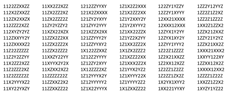
For each of the remaining choices of EPR-pairs we numerically examined all Pauli measurement bases on qubits and computed the final post-measurement state of qubits using the standard stabilizer formalism. To test whether the final state is locally equivalent to the desired EPR-pairs, we checked whether the entanglement entropies of the final state obey and for . The entanglement entropy of a stabilizer state can be extracted from its tableaux as described in [FCY+04]. Any two-qubit stabilizer state of qubits satisfying and has to be maximally entangled and thus equivalent to the EPR-pair modulo single-qubit Clifford gates. We found a Pauli basis generating maximally-entangled states on qubits and in all considered cases, see Figure 5. We also observed that the graph state is not -pairable if the Pauli bases are restricted to and only.
We verified numerically that no stabilizer state with qubits is -pairable using LOCC protocols based on Pauli measurements, by checking all possible 9-qubit graph states as listed in [AMSDS20]. The code is available at https://github.com/yashsharma25/generating-k-epr-pairs
4 Obstructions for complete pairings ()
Now we turn from constructions to proving limitations on all possible -pairable resource states. Let be the number of parties as in the previous sections. Since we are talking about complete pairings in this section, we assume here that is divisible by 2. For a pairing
the tensor product of the EPR-pairs,
is a state on qubits, where by definition .
For our first type of lower bounds we assume that the parties want to achieve all possible complete pairings on . Then we find a super-constant lower bound on the required number of qubits per party:
Theorem 9.
Suppose is a fixed state of qubits shared by parties such that each party holds qubits of . Suppose that for any pairing of qubits a transformation is realizable by an LOCC protocol such that at the end of the protocol the -th qubit of belongs to the -th party for all , and is an arbitrary state on the qubits not belonging to .666Without loss of generality we may assume . Then
The proof of this theorem is going to be a dimension calculation, but with a twist. Given a starting state we estimate the dimension of the space that contains all those states that can be obtained (with positive probability) from by an LOCC protocol. We want to compare this with the dimension of the space induced by all possible states that should arise as output, where we let the input range over all possible pairings. This by itself, however, will not yield the desired lower bound. The mathematical idea is that rather than representing each state by itself, we represent it by its tensor power, where will be carefully set in the magnitude of . Let
be the linear space induced by the tensor powers of all possible output states. Before stating a lower bound on we prove a lemma:
Lemma 10.
Let and be two pairings. Then , where is the number of cycles in , as a graph on vertex set .
Proof.
Note that the graph (the union of the two perfect matchings and on the same vertex set ) is a collection of cycles. We have
where is the set of binary strings, corresponding to the vertex labeling of the graph such that for every we have , and for every we have . In other words, the labeling must be constant on each connected component of . Therefore,
∎
Lemma 11.
There exist constants such that
Proof.
Let , . Let
We define an undirected graph on by
Let us view each as a 1-1 map from to . Then if and only if is a permutation on with at least cycles. If we fix , then as varies, runs through all permutations of . Thus, every vertex of has degree , where is the number of permutations of having at least cycles. Let be the unsigned Stirling numbers of the first kind. It is known that is exactly the number of permutations of elements with disjoint cycles. Thus
It is also known that
The right-hand side above is at most
Therefore:
Then,
implying the existence of an independent set in of size at least by a well-known greedy argument: pick a vertex to add to the independent set, remove it and its neighbors, and continue with the remaining graph. Using Stirling’s formula to estimate the factorials, there is a (, when ) such that . Let be an independent set in of size (we ignore rounding to an integer for simplicity). Define the linear space
From now on we set , where (, when ). It is enough to show that we have (), since . Let us define the Gram matrix of the system:
For it is sufficient to show that has full rank.
Gershgorin’s circle theorem implies, for any (complex) square matrix : if for all indices , then has full rank.
In order to apply this theorem, we compute for the -row of our matrix :
where we used Lemma 10. Since in addition, for all , Gershgorin’s circle theorem implies that our matrix has full rank. Hence . ∎
Lemma 11 says that for any fixed state , the possible outputs (over all input pairings ), when taking their tensor power with , should span a space of dimension .
This number we have to compare with the dimension of the span of tensor powers of possible states that can be produced by an LOCC protocol from . Although LOCC protocols may use unlimited classical communication, they cannot create new entanglement, so all entanglement in their final state is a local linear transformation of the entanglement that already existed in the starting state .
When each party only possesses qubits, where is very small, the variety of states that an LOCC protocol can produce from is limited in the way we describe below.
To capture this limitation, notice that any LOCC protocol can be described by a completely positive trace-preserving (CPTP) map, with separable Kraus operators. It follows that for any pairing there exists a product Kraus operator
| (24) |
such that maps qubits to one qubit for all and for all pairings :
| (25) |
Define:
where the are arbitrary operators mapping qubits to one qubit ( may depend on ), and is our fixed starting state. From Equations (25) and (24) we get the subspace inclusion
and hence, using Lemma 11, for some we have . However, when this cannot be the case because of the following upper bound:
Lemma 12.
Proof.
Linear operators that map qubits to one qubit can be considered as vectors in a complex space of dimension (use the vectorized form of operators). Crucially, the -fold tensor products live in the symmetric subspace of , which has dimension
| (26) |
(this is where the big saving occurs: without the information that the vector is in the symmetric subspace, we would have to calculate with instead of the above expression, and would get only a trivial bound). It follows that operators of the form span a linear space of operators with dimension at most
| (27) |
Thus states of the form with a fixed span a linear space with dimension upper bounded by Equation (27). Substituting , one gets the statement of the lemma. ∎
5 Obstructions for partial pairings
In this section we generalize the result of the previous section to partial pairings and show:
Theorem 13.
Let be an integer, , and be a -pairable state for parties where each party has qubits. Then
Proof.
For technical reasons we assume that is divisible by 4. In the proof we also assume that , since otherwise there is nothing to prove: the expression in parentheses on the right-hand side is always larger than . A -pairing of is
We denote the set of -partial pairings on with . As in the previous section, we assume that each party has qubits, and one of these is designated as the output qubit, which will hold a qubit of an EPR-pair at the end of the protocol whenever involves the party in question. The goal is to be able to produce
from some fixed initial -qubit resource state , for all . We note that in the above tensor product the listing order of the qubits depends on , and we list only the qubits designated to be output bits. (We list even those designated output qubits of parties that are not covered by the current partial matching , since they will participate in the output for other s.) For the remaining qubits, we assume w.l.o.g. that they end up in the -state, and hence are not entangled with the rest. To achieve this the parties can set these qubits to by a local operation.
The proof is a slight variation of our proof for the complete-pairing case. There was calculated, and similarly to the previous section this dimension upper bounds the dimension of
The calculation is very similar to the case of complete pairings:
-
1.
We will find different s such that their tensor powers, where , are linearly independent. (In the complete pairing case it was different s.)
-
2.
Setting is still the only reasonable choice. Further, the approach breaks down at , so we will be satisfied with investigating . With the above parameters for and we have , hence via Lemma 12 we have:
-
3.
Similarly to our argument in the previous section, the dimension of must lower bound the dimension of , which is .
-
4.
Combining 1 and 3, we get ), which implies Theorem 13.
Points 2-4 require no explanation as they just reiterate ideas of the previous section. However, we need to prove Point 1.
First we prove the analogue of Lemma 10 for partial pairings.
Lemma 14.
Let and be two partial pairings with pairs. Then
where is the number of cycles in , as a graph on vertex set .
Proof.
We have:
where is the set of binary strings, corresponding to the vertex labeling, , of the graph such that for every we have , and for every we have and furthermore every element of vertex set that is not covered by both a -edge and a -edge (that is, elements not in ) must get label 0.777The formula for comes from computing the inner product in the most straightforward way: we notice that both and have only two kinds of entries: 0 and . Then we just identify those entries where both and are non-zero and compute the number of such entries. Thus, only the cycles in can be labeled two ways, and no more than two ways, since the edges of and force the condition that all labels over the cycle must be either 0 or 1. (Paths cannot be labeled two ways as the label at their endpoint is fixed to 0.) This calculation of gives the formula. ∎
We let , and define
Then . We need a lower bound on . Using the well-known bounds
one gets
where the second inequality follows from . We again create a graph with:
Note that is again regular as in the previous section, since it is vertex-symmetric. Like before, we want to lower bound where is the degree of a , which is then a lower bound on the size of a maximal independent set in . In fact, for an arbitrary fixed we have:
To upper bound the size of , w.l.o.g. let : we match the first vertices in the first half with the first vertices in the second half. We can upper bound the number of neighbors of by enumerating them, each possibly multiple times. To define a somewhat elaborate enumeration, first notice that the nodes of any cycle in must be fully contained in the vertex set . Assume is a neighbor of such that has cycles. Pick an (arbitrary) point in every cycle, such that the selected points belong to . Let these points be , and let
Let be the length of the cycle that goes through (all cycles have even length, because the edges alternate between and ), and denote:
Since , we have . Finally, let us define
The triplet with one piece of additional information, which will be defined next, will determine . The number of triplets is , since all three of can be given as subsets of sets of size at most (e.g., is a subset of due to ).
Let us now understand the magnitude of the additional information888We could have chosen information-theoretic terminology for our explanation, where we relate the ratio to the mutual information between and . We have opted for an equivalent counting explanation, but the reader has to bear in mind, that our underlying intuition is that every cycle that and jointly create, increases their mutual information by bits (essentially, the edge of that “closes the cycle” is cheap to communicate, given ). The ratio is simply the exponential of this mutual information. that together with determines . It will turn out that this information is bits, where very crucially, is less than 1 (in fact, will be essentially ). This implies an upper bound on , which in turn implies the following lower bound on the size of the largest independent set in :
| (28) |
Additional data that with uniquely determines , given that is ’s neighbor in :
We shall define an order of edges of . We will denote the -endpoint of by .
Before telling the order, note that the cycles in already have a natural order, modulo the information, namely the cycle is the cycle that contains . To “extend” this order to the edges we introduce:
-
1.
Among all edges of those edges come earlier that are edges of some cycle.
-
2.
If two edges both participate in a cycle, but these two cycles are different, then the edge comes first that belongs to an earlier cycle.
We need to tell how to order edges within the same cycle. Also, we need to tell how to order edges that do not belong to any cycle.
Ordering of edges of that belong to a given cycle.
If the cycle is the
cycle, we simply walk through the
the cycle and order the -edges as we encounter them.
The walk-through starts from with a -edge (which determines that in which orientation
we follow the cycle).
For instance, consider the first cycle.
For this example notice that if is a cycle-edge
in , then belongs to the same cycle as .
We get:
| is the edge of with -endpoint | |
| is the edge of with -endpoint | |
| is the edge of with -endpoint | |
| is the edge of with -endpoint |
Ordering of edges of that do not belong to any cycle:
These edges are simply ordered by the numerical value of their -endpoints: edges with a smaller -endpoint come earlier.
Let us now assume that Alice has to specify to Bob. First Alice gives Bob the triplet. Then she starts to tell Bob . (Recall, is the -endpoint of .) Two remarkable observations lead to our conclusions.
-
1.
Even though Alice only tells the -endpoints to Bob, Bob will (recursively) figure out the -endpoints as well. This is in fact trivial. For instance, the -endpoint of is , which is known to Bob, since is given to him, etc. When the last cycle is exhausted, Bob knows this (this is after edges had been encountered—the total number of cycle-edges; in turn is given as the last element of the -sequence), and from then on Bob relies on to get the -endpoints.
-
2.
When Alice arrives at an edge that closes a cycle, she does not need to send the -endpoint of this edge! It is simply , if the cycle was the cycle. In other words, it is the other endpoint of the edge of incident to . Therefore, we just assume that Alice skips telling the -endpoint of the last edge of every cycle. But how does Bob know that he has arrived at the last edge of the current cycle? He knows this, because the cycle lengths are encoded in : the length of the cycle is if and for .
In summary, the information Alice gives to Bob besides to identify , is the sequence, but crucially, completely leaving out from this sequence the -endpoints of all the cycle-closing edges. We have cycle-closing edges. Describing any takes bits, since . Therefore:
The number of bits Alice needs to send Bob to fully describe a that creates cycles with is:
In conclusion, the number of different s that form cycles with can be upper bounded by . To upper bound , recall that is allowed to vary from to , so is upper bounded by . Thus, looking back at Eq. (28) and using that , there exists an independent set of size in . Consequently, we can find a set of that many partial permutations such that if belongs to this set, then the inner product of and is at most . Setting to be (generously, in fact: we care only about the case, hence the factor becomes ) and applying Gershgorin’s circle theorem in the same fashion as in the proof of Lemma 11 in the previous section, we prove Point 1 and conclude the proof of Theorem 13. ∎
Theorem 13 has the following consequence for the case where each party is restricted to a constant number of qubits:
Corollary 15.
Let be a -pairable state for parties where each party has qubits. Then .
As mentioned in the introduction, up to the power of the polylog this matches our expander-based construction of -pairable states where and (Corollary 3).
6 Conclusion and future work
In this paper we initiated the study of -party resource states from which LOCC protocols can create EPR-pairs between any disjoint pairs of parties. These EPR-pairs then enable quantum communication over a classical channel via teleportation. Our focus was on the tradeoff between the number of to-be-created EPR-pairs (which we want to be large) and the number of qubits per party (which we want to be small).
This work leaves open several questions for future work:
-
•
Our constructions of -pairable states may be far from optimal, and it would be interesting to improve them. For example, it might be possible to significantly reduce the number of qubits of our Reed-Muller-based construction of -pairable states with one qubit per party. Also, the case remains largely open since two qubits per party is not enough to realize entanglement swapping protocols on expander graphs, see Section 2. All our constructions are based on stabilizer-type resource states. Can one improve the tradeoff between and using more general resource states? Can one express the pairability parameter in terms of some previously studied entanglement measures?
-
•
Regarding lower bounds (obstructions), we showed in Section 4 that a resource state for complete pairings () requires qubits per party. Can we improve this lower bound to qubits, matching the upper bound we obtained from expander graphs at the end of Section 2? Our lower bounds are actually for a stronger model, applying to LOCC protocols that produce the desired state with positive probability; there may be better upper bounds in this setting, and/or stronger lower bounds for LOCC protocols that are required to succeed with probability 1.
-
•
How well do our resource states behave under noise? Contreras-Tejada, Palazuelos, and de Vicente [CPdV22] already proved some negative results here for the type of constructions we gave in Section 2 (with EPR-pairs on the edges of an -vertex graph), showing that genuine multipartite entanglement only survives constant amounts of noise per edge if the graph has a lot of connectivity.
-
•
We can ask a very similar classical question, where the classical analogue of an EPR-pair is a uniform bit shared between two parties and unknown to all others. Such shared secret bits can then be used for secure communication over public classical channels (via the one-time pad), similarly to how shared EPR-pairs can be used for secure quantum communication over public classical channels (via teleportation). We believe our techniques can be modified to obtain non-trivial results about the question: what classically correlated -party resource states are necessary and sufficient for LOCC protocols (with public classical communication) to generate such secret shared bits between any disjoint pairs of parties? One difference is that the straightforward classical analogue of the GHZ-state (a uniformly random bit known to all parties) is not 1-pairable in this classical sense.
Acknowledgements.
References
- [AG04] Scott Aaronson and Daniel Gottesman. Improved simulation of stabilizer circuits. Physical Review A, 70(5):052328, 2004.
- [AJ92] E. F. Assmus Jr. On the Reed-Muller codes. Discrete mathematics, 106:25–33, 1992.
- [AMSDS20] Jeremy C. Adcock, Sam Morley-Short, Axel Dahlberg, and Joshua W. Silverstone. Mapping graph state orbits under local complementation. Quantum, 4:305, 2020.
- [BBC+93] Charles Bennett, Gilles Brassard, Claude Crépeau, Richard Jozsa, Asher Peres, and William Wootters. Teleporting an unknown quantum state via dual classical and Einstein-Podolsky-Rosen channels. Physical Review Letters, 70:1895–1899, 1993.
- [BFU94] Andrei Z. Broder, Alan M. Frieze, and Eli Upfal. Existence and construction of edge-disjoint paths on expander graphs. SIAM Journal on Computing, 23(5):976–989, 1994.
- [Bol88] Béla Bollobás. The isoperimetric number of random regular graphs. European Journal of combinatorics, 9(3):241–244, 1988.
- [CPdV22] Patricia Contreras-Tejada, Carlos Palazuelos, and Julio I. de Vicente. Asymptotic survival of genuine multipartite entanglement in noisy quantum networks depends on the topology. Physical Review Letters, 128:220501, 2022. arXiv:2106.04634.
- [CRSS98] A. R. Calderbank, E. M. Rains, P. W. Shor, and N. J. A. Sloane. Quantum error correction via codes over GF(4). IEEE Transactions on Information Theory, 44(4):1369–1387, 1998.
- [CS96] A. Robert Calderbank and Peter W. Shor. Good quantum error-correcting codes exist. Physical Review A, 54(2):1098, 1996.
- [DHW18] Axel Dahlberg, Jonas Helsen, and Stephanie Wehner. How to transform graph states using single-qubit operations: computational complexity and algorithms, 2018. arXiv:1805.05306.
- [DHW20] Axel Dahlberg, Jonas Helsen, and Stephanie Wehner. Transforming graph states to Bell-pairs is NP-complete. Quantum, 4:348, 2020.
- [DSL17] Gang Du, Tao Shang, and Jian-Wei Liu. Quantum coordinated multi-point communication based on entanglement swapping. Quantum Information Processing, 2017.
- [FCY+04] David Fattal, Toby S. Cubitt, Yoshihisa Yamamoto, Sergey Bravyi, and Isaac L. Chuang. Entanglement in the stabilizer formalism, 2004. quant-ph/0406168.
- [FT21] Alex Fischer and Don Townsley. Distributing graph states across quantum networks. In Proceedings of IEEE International Conference on Quantum Computing and Engineering (QCE), 2021. arXiv:2009.10888.
- [GMM17] Ervin Győri, Tamás Róbert Mezei, and Gábor Mészáros. Note on terminal-pairability in complete grid graphs. Discrete Mathematics, 340(5):988–990, 2017.
- [Got98] Daniel Gottesman. The Heisenberg representation of quantum computers. arXiv preprint quant-ph/9807006, 1998.
- [HPE19] Frederik Hahn, Anna Pappa, and Jens Eisert. Quantum network routing and local complementation. npj Quantum Information, 5(1):1–7, 2019.
- [IVK+22] Jessica Illiano, Michele Viscardi, Seid Koudia, Marcello Caleffi, and Angela Sara Cacciapuoti. Quantum internet: from medium access control to entanglement access control. arXiv:2205.11923, 2022.
- [MMG19] Clément Meignant, Damian Markham, and Frédéric Grosshans. Distributing graph states over arbitrary quantum networks. Physical Review A, 100(052333), 2019. arXiv:1811.05445.
- [MPD23] Jorge Miguel-Ramiro, Alexander Pirker, and Wolfgang Dür. Optimized quantum networks. Quantum, 7:919, 2023. arXiv:2107.10275.
- [MS77] Florence Jessie MacWilliams and Neil James Alexander Sloane. The theory of error correcting codes, volume 16. Elsevier, 1977.
- [NC02] Michael A. Nielsen and Isaac Chuang. Quantum computation and quantum information. Cambridge University Press, 2002.
- [PKT+19] Mihir Pant, Hari Krovi, Don Towsley, Leandros Tassiulas, Liang Jiang, Prithwish Basu, Dirk Englund, and Saikat Guha. Routing entanglement in the quantum internet. npj Quantum Information, 5(1):1–9, 2019.
- [RBB03] Robert Raussendorf, Daniel E. Browne, and Hans J. Briegel. Measurement-based quantum computation on cluster states. Physical review A, 68(2):022312, 2003.
- [SMI+16] Eddie Schoute, Laura Mančinska, Tanvirul Islam, Iordanis Kerenidis, and Stephanie Wehner. Shortcuts to quantum network routing. arXiv:1610.05238, 2016.
- [Ste96] Andrew Steane. Multiple-particle interference and quantum error correction. Proceedings of the Royal Society of London. Series A: Mathematical, Physical and Engineering Sciences, 452(1954):2551–2577, 1996.
- [WEH18] Stephanie Wehner, David Elkouss, and Ronald Hanson. Quantum internet: A vision for the road ahead. Science, 362(6412), 2018.
Appendix A Constructing an that satisfies condition CSS1, when all , are independent
In this appendix we give a proof for a simpler but instructive special case of how we satisfy CSS1 in Section 3.6. The additional assumption of our special case is to suppose that are linearly independent.
Let be the linear subspace of spanned by and (so in particular, ). Let be (mod 2) variables. Then the above vectors define linear functions over : every vector can be uniquely written as
for some binary coefficients that are functions of . As such, all these functions are linear, since when writing down as above, we add the corresponding coefficients. In the sequel we shall create higher-degree polynomials over from these linear functions (e.g., is a quadratic function).
Let . Note that . Condition CSS1 (with ) asks for a degree- polynomial such that
| (29) |
Let us show that Eq. (29) is satisfied if we choose as
| (30) |
where
| (31) |
The polynomial defined in Eq. (30) has degree , because has degree 1 and has degree . However, we will see that the restriction of onto coincides with a degree- polynomial.
First, we show that
Indeed, extending the sum over in Eq. (31) to all subsets would give a function which is zero mod 2 unless for all . The missing monomial associated with the subset is zero unless for all .
By definition of , any vector can be written as a sum of an odd number of vectors from the set . In particular, for any . Thus the restriction of onto is zero unless for all . In the latter case one has or for some . If then since . If then since . This proves Eq. (29).
Next we claim that degree- monomials in can be replaced by monomials of degree at most without changing the restriction of onto . Indeed, the sum of all degree- monomials in can be written as
| (32) |
Supose . We claim that iff or . Indeed, if for then since . Suppose . Then and thus . By definition of , one can write as a sum of an odd number of vectors from the set . Hence iff or .
If is even then none of the vectors and belongs to . Thus for all . If is odd, the same arguments as above show that
| (33) |
Thus we can replace by a monomial of degree either zero (if is even) or degree (if is odd) without changing the restriction of onto . This proves condition CSS1.
A numerical example: Let , , and let
| 000010000000 | |
| 000001000000 | |
| 000000100000 | |
| 000000010000 | |
| 000000001000 | |
| 000000000100 | |
| 000000000010 | |
| 000000000001 |
We also set for , so , etc. To address condition CSS1 for we want to write down a degree-3 polynomial over that on the set takes value 1 on and , and 0 on the rest of . (By symmetry then we can write down similar functions for .) Let be the Hamming weight of the first 4 bits of and let be the Hamming weight of the last 8 bits of . Notice that for all we have and , and even within this restriction some weight combinations may never arise for any element of . Such weight combinations we will call “impossible pairs.” For each weight combination we have calculated the number of elements of EZ that have that weight combination, see the table below. We put an asterisk (rather than 0) in the entries that represent impossible weight combinations.
| 0 | 1 | 2 | 3 | |
|---|---|---|---|---|
| 0 | 4 | 4 | ||
| 1 | 8 | 24 | ||
| 2 | 12 | 4 |
The entries are not hard to calculate, and to give a typical example we calculate the -entry: There are 8 weight-1 strings of the last 8 bits, and 6 weight-2 strings of the first 4 bits. However, not all elements of the set can be added to some element of the set . For instance does not occur in , as does not contain . It is easy to see that these bad combinations are half of all possible combinations, hence we obtain 24 as the -entry of the table.
Observe now that , so Lemma 5 cannot be applied directly to get a degree-3 polynomial. Let us now construct a degree-3 polynomial that restricted to satisfies condition CSS1 for . First note that satisfies CSS1 for if
Consider now the polynomial
One can easily check that
| When | 0 | 1 | 2 | 3 | |
| then mod 2 | 1 | 0 | 0 | 1 |
and that the polynomial then takes values on exactly as needed. (For instance, when and then will always give zero, etc.)
Appendix B Induction step of Section 3.6: modifications for odd
Here we extend the proof of -pairability given in Section 3.6 to odd values of . Suppose is an integer. We say that a family of polynomials labeled by subsets with is valid if it satisfies the following conditions.
-
I1:
depends only on the variables
-
I2:
has degree
-
I3:
and for
-
I4:
for any non-empty set and any
-
I5:
if is odd and
-
I6:
if and
-
I7:
if and
These conditions are identical to the ones given in Section 3.6, except for condition (I7) which is now imposed only for . Below we assume that is odd. As before, we shall use induction on to prove that a valid family of polynomials exists for all .
The base of induction is . Then a valid family is a single polynomial . The construction of is identical to the one given in Section 3.6.
We shall now prove the induction step. Suppose we have already constructed a valid family of polynomials with . Consider a subset with such that . The case will be considered afterwards.
Suppose is odd. Condition (I2) demands that has degree . Condition (I3) can be skipped since . Consider two cases.
Case 1: . Then (I5) demands . This automatically satisfies (I6,I7). It remains to check (I4) which is equivalent to
| (34) |
for . Note that consists of points and with . All terms with odd vanish due to (I5). All terms with even obey (I6). Since , we have and due to (I6). Thus all terms vanish, that is, Eq. (34) is satisfied.
Case 2: . Then since both and are odd. We can skip (I5,I6,I7). Thus we just need to satisfy (I4). It fixes the values of at points, namely, and with . Since , the desired polynomial exists by part (1) of Lemma 5.
Suppose is even. Condition (I2) demands that has degree . Conditions (I3),(I5) can be skipped since is even and . We claim that (I7) follows from (I4). Indeed, we have iff or with . We have due to (I4). If is odd then due to (I5) since . If is even then . Thus since (I7) holds for . This implies for any , as claimed in (I7). It remains to check (I4,I6). We fix the value of at points in (I4) if . We fix the value of at points in (I4,I6) if . Consider first the case . Then since is odd, is even, and . Thus . Part (1) of Lemma 5 implies that the desired polynomial exists. Next consider the case . Then . Part (1) of Lemma 5 implies the desired polynomial exists.
It remains to prove the induction step for . Suppose we have already constructed a valid family of polynomials with . Consider a subset with . Since we assumed that is odd, is even. Condition (I2) demands that has degree , that is, is a constant function. We can skip conditions (I3,I5,I6,I7) since none of them applies if . It remains to check (I4). Note that for some such that . Condition (I4) fixes the value of at and . Since we want to be a constant function, it suffices to check that the desired values and are the same. Substituting the desired values from (I4), we have to check that
| (35) |
All terms with vanish since obeys (I7). Thus we can restrict the sum Eq. (35) to terms with . However is a degree-1 polynomial if due to (I2). Thus and Eq. (35) is equivalent to
| (36) |
Since obeys (I4) and is odd, we have for or . Thus Eq. (36) is equivalent to
| (37) |
All terms with odd vanish due to (I5) since . All terms with even and vanish due to (I6). Thus we can restrict the sum Eq. (37) to terms with and it suffices to check that
| (38) |
However, each term and is counted exactly two times: if then one can choose or . Since we do all arithmetic modulo two, this implies Eq. (38). Thus (I4) is satisfied. This completes the induction step for odd .
