More Generalized and Personalized Unsupervised Representation Learning In A Distributed System

Abstract

Discriminative unsupervised learning methods such as contrastive learning have demonstrated the ability to learn generalized visual representations on centralized data. It is nonetheless challenging to adapt such methods to a distributed system with unlabeled, private, and heterogeneous client data due to user styles and preferences. Federated learning enables multiple clients to collectively learn a global model without provoking any privacy breach between local clients. On the other hand, another direction of federated learning studies personalized methods to address the local heterogeneity. However, work on solving both generalization and personalization without labels in a decentralized setting remains unfamiliar. In this work, we propose a novel method, FedStyle, to learn a more generalized global model by infusing local style information with local content information for contrastive learning, and to learn more personalized local models by inducing local style information for downstream tasks. The style information is extracted by contrasting original local data with strongly augmented local data (Sobel filtered images). Through extensive experiments with linear evaluations in both IID and non-IID settings, we demonstrate that FedStyle outperforms both the generalization baseline methods and personalization baseline methods in a stylized decentralized setting. Through comprehensive ablations, we demonstrate our design of style infusion and stylized personalization improve performance significantly.

Introduction

Deep learning models are growing exponentially over the demand on endless data. In a centralized setting, all data is accessible to train a deep learning model at a massive scale. However, with the emerging of edge devices, it is more desirable to train a small-sized deep learning model on local training data and aggregate local models to form a global model for a new deployment. McMahan et al. (2017) proposes federated learning that enables multiple local clients to collectively train a global model in a iterative updating process without sharing local training data between clients. By labelling each example generated on a local device, federated learning has demonstrated competitive performances on various computer vision tasks (Li et al. 2019; Liu et al. 2020; Long, Shelhamer, and Darrell 2015). However, manually labeling all data from numerous local devices is increasingly expensive and concerns users with privacy issue. This substantial requirement leaves most of data on local devices unlabeled. Additionally, data collected and accessible locally is very user-centered, which induces high data heterogeneity across devices due to distinctive user style and preference. Figure 1 depicts the learning process on user-centered unlabeled data in a distributed environment.

Figure 1: Federated unsupervised representation learning with stylized user data. Distinctive user style and preference introduce data heterogeneity and lead to deteriorated global generalization and local personalizations.

In the absence of labeled training data, Self-Supervised Learning (SSL) has been developed to pretrain a model with unlabeled data and learn visual representations that are well-generalized to downstream tasks. Discriminative and generative self-supervised methods received growing attentions in recent years (Chen et al. 2020a, b; Donahue and Simonyan 2019; Gidaris, Singh, and Komodakis 2018; Jaiswal et al. 2020; Zhang, Isola, and Efros 2016; He et al. 2022). Contrastive learning has become the most popular discriminative SSL method that either computes InfoNCE (Oord, Li, and Vinyals 2018) on positive and negative examples (Chen et al. 2020a, b) or predicts projected latent of only positive examples (Grill et al. 2020; Chen and He 2021; Zbontar et al. 2021). The success of the contrastive learning on visual datasets engenders research and study about applying such a method to other formats of data, such as audio data (Saeed, Grangier, and Zeghidour 2021) and medical data (Mohsenvand, Izadi, and Maes 2020). However, the effectiveness of the method in a distributed environment seeks further study.

Applying contrastive learning in a distributed system with stylized local data poses two core challenges. First, without any supervision, learning a generalized global model is more difficult when all local data is diverse in distribution and limited in volume. Second, while securing a generalized global model, customizing personalized local models is also harder when local data is dispersed not only in class distribution but also in style. These two obstacles require completely different treatments to resolve. Generalization involves a strong regularization to align different local models whilst personalization weakens such regularization to promote customized fit on local dispersed data.

Figure 2: Intuition of style infusion to improve representations via contrastive learning.

In this work, we address both generalization and personalization of the federated unsupervised representation learning with the utilization of local style information. In (Von Kügelgen et al. 2021), authors assume that an image is generated by a content factor ($c$) and a style factor ($s$). The authors further prove that, under a self-supervised learning framework, the feature extractor learns content-identifiable representations that are robust to augmentations applied (upper part of Figure 2). Based on this argument, our intuition is that a locally extracted image feature is a product of a generalized content feature ($h_{c}$) and a personalized style feature ($h_{s}$). During self-supervised learning, the content feature is infused with locally extracted style features so that the learned representation is also robust to this latent distortion (lower part of Figure 2). Since every client has its own style and preference, infusing extracted local style features into global content features and facilitating personalized features in a decentralized setting become feasible to achieve good results in both generalization and personalization. We propose Federated with Style (FedStyle) via training a local style feature extractor and combining a content feature extracted via a local content model with the style feature to generate a style-infused representation for contrastive learning. This incorporation of style and content features empowers the local content models to be robust to local distortion in addition to other image-level distortions applied for contrastive learning (Chen et al. 2020a). With local models robust to local distortions, a generalized global model robust to various distortions can be aggregated. When deploying on downstream tasks, apart from the generalized content feature, a stylized content feature is also used to promote personalization.

With extensive experiments, we evaluate the effectiveness of FedStyle in terms of generalization and personalization under both IID and non-IID data distributions. To simulate user-centered data style, we evaluate FedStyle on three different data types: 1. Digit consisting MNIST (Deng 2012), USPS (Hull 1994), and SVHN (Netzer et al. 2011); 2. Office Home (Venkateswara et al. 2017) consisting Art, Clipart, Product, and Real World styles; 3. Adaptiope (Ringwald and Stiefelhagen 2021) consisting Synthetic, Product, Real Life styles. FedStyle delivers a more generalized global model than the FedAvg baseline and achieves higher personalized accruacy than personalized federated algorithms: FedRep (Collins et al. 2021), FedPer (Arivazhagan et al. 2019), FedProx (Li et al. 2020), APFL (Deng, Kamani, and Mahdavi 2020), and Ditto (Li et al. 2021).

Related work

Unsupervised Representation Learning, URL, aims to learn generalized data representations from unlabeled data. Self-supervised Learning (SSL) designs pretext tasks based on either easily constructed labels (discriminative) or reconstructions of original data (generative). Before the surge of contrastive learning, discriminative SSL methods train on manually constructed labels such as colors (Zhang, Isola, and Efros 2016), rotations (Gidaris, Singh, and Komodakis 2018), positions of split patches (Noroozi and Favaro 2016), etc. Contrastive Learning, CL, relies on a simple idea that different views of the same data example should be as similar as possible. In other words, the representation of an image should be robust to any distortions applied to the image’s appearance. Many CL approaches compute the InfoNCE loss (Oord, Li, and Vinyals 2018). Minimizing the loss pulls representations of similar/positive examples closer and pushes representations of dissimilar/negative examples further in the latent space. Chen et al. (2020a) formulates augmented views of the same image as positive examples and all other representations in a mini training batch as negative examples. Chen et al. (2020b) recognizes the same positive examples but adopts a memory bank to store many momentum-updated representations as negative examples. Other CL methods exclude the notion of negative examples and only predict positive representations from a projected view (BYOL (Grill et al. 2020) and SimSiam (Chen and He 2021)) or reduce redundancy in the feature dimension space (Barlow Twin (Zbontar et al. 2021)).

Federated Unsupervised Representation Learning, FURL, adapts URL in a distributed system that learns a common representation model without supervision while preserving data privacy. Federated Learning allows selected local models to be trained on local data and aggregates these local models to form a global model in a iterative communication process. In the absence of labeled data, unsupervised representation learning such as contrastive learning is applied to the distributed system. However, simply aggregating local models causes deterioration in performances due to local data heterogeneity and small local training size. Methods have been developed to mitigate the deterioration. FedCA (Zhang et al. 2020) utilizes a dictionary storing representations from clients to address the heterogeneity and an alignment model trained on a public dataset on the server to address the misalignment. FedU (Zhuang et al. 2021) modifies BYOL that only updates the predictor of the local model if the divergence from the previous communication round is below a certain threshold. He et al. (2021) explores the flexibility of centralized CL methods in the distributed system and emphasizes the personalization of local models by updating global parameters locally and updating local parameters separately. Wu et al. (2021) proposes the fusion of features from other clients to reduce the false negative ratio and feature space matching of neighbouring clients to alleviate misalignment. Nonetheless, these methods may violate the user privacy protocol as they share information between local clients, or they require extraneous architecture for each client, which increases the memory burden at clients’ ends. Furthermore, the aforementioned methods do not address both global generalization and local personalizations and do not apply to more than one contrastive learning algorithm.

Personalized Federated Learning, PFL, focuses on better local performances with auxiliary local architecture or information. Aggregating diverse local models trained on heterogeneous data causes a slow convergence of the global model and results in poor local performances. Multitask-learning-based PFL (Dinh et al. 2021; Marfoq et al. 2021) trains a personalized model for each client by considering each client as a different task and computing similarity between pairwise client relationships. Clustering-based PFL (Sattler, Müller, and Samek 2020; Briggs, Fan, and Andras 2020) clusters local models based on group-level client relationships and adapts new client models based on the clusters. Meta-learning-based PFL (Fallah, Mokhtari, and Ozdaglar 2020; Khodak, Balcan, and Talwalkar 2019) adapts the global model to a personalized model by finetuning locally. However, the aforementioned types of PFL require extra computational power to compute similarity or finetuning, and this requirement slows down the learning process. Without labeled data, unsupervised learning expects an even longer training time to yield good performance. Model-based PFL learns a global model for the common knowledge while learning local models for local knowledge. To learn the local model only requires regularization to the global model or partial local model update on the fly. FedPer (Arivazhagan et al. 2019) only updates the base of the global model at local ends while finetunes the MLP classifier locally. FedRep (Collins et al. 2021) trains the encoder and the classifier separately for different local epochs and only aggregates the local base encoders on the server. APFL (Deng, Kamani, and Mahdavi 2020) learns a convex mixture of a local and a global model as the personalized model. FedProx (Li et al. 2020) regularizes the local model to the current global model to avoid fast divergence while allowing the local model to converge better on local data. Ditto (Li et al. 2021) extends FedProx by optimizing the global model locally and regularizing the local model to the optimized global model. We compare with these model-based PFL methods as the proposed method includes a style model as the local model and the training involves two models.

Federated with Style (FedStyle)

Under a decentralized system with unlabeled local data, we adapt unsupervised representation learning to train a generalized global model. Figure 3(a) demonstrates three components of the proposed method. We propose to extract local style information by contrasting local original images with sobel filtered images (3(a)). We propose to improve the generalization of the global model by importing the style information for a style infusion (3(b)) that is beneficial to unsupervised representation learning. And we propose improve personalization of the local models via stylized content features (3(c)) that are tailored to local heterogeneous data. Additionally, we provide an analysis of the effectiveness of proposed style-infused loss on learning better representations.

(a) Local Style Extraction

(b) Local Style Infusion

(c) Personalization

Figure 3: Proposed FedStyle process: (a) Extract local style by contrasting original with the Sobel filtered images. (b) Infuse local style feature with the content feature for contrastive learning. (c) Impart both content feature and stylized content feature for personalized tasks.

     

Problem Setting In a distributed system, there are $N$ clients. The current global model weight is updated to a set $\{C\}$ containing $\alpha$ portion of total clients at each communication round. Each selected client, $k\in\{C\}$, trains a model with weights $w_{k}$ on local data $\mathcal{D}_{k}$ for $E_{l}$ local epochs. After local training, the selected clients send $w_{k}$ to the server, and the server aggregates it as a global model with weights $w$. This process is repeated for $E_{g}$ communication rounds. The overall goal is to minimize:

$$\min_{w}\mathcal{L}(w)=\frac{1}{n}\sum_{k=1}^{n}\mathcal{L}_{k}(w,\mathcal{D}_{k}),$$ (1)

where $\mathcal{L}_{k}(w,\mathcal{D}_{k})$ is the local loss of client $k$ on data distribution $\mathcal{D}_{k}$. In this problem, we assume each $\mathcal{D}_{k}$ has an user style $s_{k}$. The federated unsupervised representation learning approach trains a local content model to compute a local loss and averages local content models on the server. Algorithm 1 outlines the overall process of federated unsupervised representation learning.

Algorithm 1 Federated unsupervised representation learning algorithm. $*$ denotes a federated learning method (FedAvg, FedRep, FedProx, FedPer, APFL, Ditto, FedStyle)

Input: Server global model, $w$. Number of clients, $N$. Client local models, $w_{k}$. Local data distribution, $\mathcal{D}_{k}$. Communication rounds, $E_{g}$. Local training epochs, $E_{l}$. Client sample ratio, $\alpha$. Method arguments, $args$.

1:Initialize $w$, $w_{k,k\in{[1:N]}}$.

2:for $round=1:E_{g}$ do

3:   Sample $K=\lfloor{\alpha\times{N}}\rfloor$ clients set $\{C\}$.

4:   for $i\in\{C\}$ do

5:      $LocalUpdate_{*}$($w$,$w_{i}$)

6:      for $epoch=1:E_{l}$ do

7:         minimize $\mathcal{L}_{i}\leftarrow$$LocalTraining_{*}$($w_{i}$,$\mathcal{D}_{i}$,$args_{*}$)

8:      end for

9:   end for

10:   $w=\sum_{k\in{\{C\}}}\frac{1}{|\mathcal{D}_{k}|}w_{k}$ // global aggregate

11:end for

Local style extraction

We propose to extract local style information for each client by contrasting original local data with a Sobel filtered (Kanopoulos, Vasanthavada, and Baker 1988) data which is a strong augmentation with a consistent and distinctive style. (Figure 3(a) as a visual description). This consistent style serves as a reference across clients to isolate user styles without sharing local information. Each client is equipped with a style model, $f_{w_{s}}$, and a style projector, $g_{w_{s}}$, to extract a style representation $\mathbf{z}_{s}$ from each data $\mathbf{x}$. $\mathbf{z}_{s}=g_{w_{s}}(f_{w_{s}}(\mathbf{x}))$. To contrast local style $s_{k}$ with the Sobel filtered style, we compute a supervised InfoNCE loss to separate local style representations from the Sobel style representations. Furthermore, InfoNCE maximizes the mutual information between data with the same local style (Tschannen et al. 2019) hence the extracted style representations contain as much local information as possible. The style loss of a mini-batch $\mathbf{x}_{\mathcal{B}}\sim{\mathcal{D}_{k}}$ is:

$$\mathcal{L}_{style}(\mathbf{x}_{\mathcal{B}}) =\sum_{\mathbf{x}_{i}\in{\mathbf{x}_{\mathcal{B}}},i=1}^{2B}\frac{1}{2B-1}\sum_{\mathbf{x}_{j}\in{\mathbf{x}_{\mathcal{B}}},j=1}^{2B}\mathbf{1}_{i\neq{j}}\cdot\mathbf{1}_{s_{i}=s_{j}}$$ (2)

$$\cdot-log\frac{exp(\mathbf{z}_{i}\cdot{\mathbf{z}_{j}}/\tau)}{\sum_{n=1}^{2B}\mathbf{1}_{i\neq{n}}\cdot{exp(\mathbf{z}_{i}\cdot{\mathbf{z}_{n}/\tau})}},$$

where $B=|\mathbf{x}_{\mathcal{B}}|$, $\mathbf{z}_{i}=g_{w_{s}}(f_{w_{s}}(\mathbf{x}_{i}))$ and $\tau$ is a temperature term. Each image $x_{i}$ in the mini-batch is processed via a Sobel filter and this doubles the total number of images in the mini-batch. In the end, $2B$ images have two styles with an equal number. Minimizing (2) will maximize the similarity between representations of the same style. A detailed style extraction procedure is listed in Algorithm 2.

Algorithm 2 Local style extraction algorithm.

Input: Local style model, $f_{w_{s},k}$. Local style projector, $g_{w_{s},k}$. Local data distribution, $\mathcal{D}_{k}$. Local style extraction epochs, $E_{s}$.

1:for epoch=1:$E_{s}$ do

2:   for mini batch $\mathbf{x}_{\mathcal{B}}\sim{\mathcal{D}_{k}}$ do

3:      for $\mathbf{x}_{i}\sim\mathbf{x}_{\mathcal{B}}$ do

4:         $\mathbf{h}_{s,i}\leftarrow{f_{w_{s}}(\mathbf{x}_{i})}$, $\mathbf{h}_{sobel,i}\leftarrow{f_{w_{s}}(Sobel(\mathbf{x}_{i}))}$

5:         $\mathbf{z}_{s,i}\leftarrow{g_{w_{s}}(\mathbf{h}_{s,i})}$, $\mathbf{z}_{sobel,i}\leftarrow{g_{w_{s}}(\mathbf{h}_{sobel,i}))}$

6:      end for

7:      $g_{w_{s}},f_{w_{s}}\leftarrow{backward(\mathcal{L}_{style}(\mathbf{x}_{\mathcal{B}}))}$

8:   end for

9:end for

Local style infusion for contrastive learning

With a style model, each client can extract local style for each local data point. By infusing the extracted local style feature with the generalized content feature, we allow the content model to be also robust to local style distortion. Therefore, we can obtain a more generalized global model when aggregating improved local content models. The process is described in Figure 3(b). To combine the style feature with the content feature and generate a style-infused content feature, we apply a non-linear MLP as a generator $G_{w_{g}}$ that takes the concatenation of the content feature and the style feature as inputs. $\mathbf{h}_{c^{\prime}}^{*}=G_{w_{g}}(\textit{concat}[\mathbf{h}_{c}^{*},\mathbf{h}_{s^{\prime}}])$. The style-infused feature is passed to the content projector, $g_{w_{c}}$, and we compute a style-infused unsupervised loss based on the output of $g_{w_{c}}$. The total loss of local training is:

$$\mathcal{L}=\mathcal{L}_{unsup}(g_{w_{c}}( \mathbf{h}_{c}^{1}),g_{w_{c}}(\mathbf{h}_{c}^{2}))+$$ (3)

$$\lambda\times\mathcal{L}_{unsup}(g_{w_{c}}(\mathbf{h}_{c^{\prime}}^{1}),g_{w_{c}}(\mathbf{h}_{c^{\prime\prime}}^{2})),$$

where $\mathcal{L}_{unsup}$ can be any general contrastive learning algorithm (SimCLR, MoCo, SimSiam, BYOL, Barlow Twins, etc.), and $\lambda$ is a scale factor modulating the effect on the style-infused unsupervised learning loss. A detailed algorithm is outlined in Algorithm 3. The clients in FedStyle only transmit local content models to the server. The overall FedStyle algorithm is listed in Algorithm 4.

Algorithm 3 Local style infusion algorithm.

Input: Local content model, $f_{w_{c},k}$. Local content projector, $g_{w_{c},k}$. Local style model, $f_{w_{s},k}$. Local generator, $G_{w_{g},k}$. Local data distribution, $\mathcal{D}_{k}$. Local unsupervised loss, $\mathcal{L}_{unsup}$. Scale on style-infused loss, $\lambda$.

1:freeze $f_{w_{s},k}$

2:for mini batch $\mathbf{x}_{\mathcal{B}}\sim{\mathcal{D}_{k}}$ do

3:   for $\mathbf{x}_{i}\sim\mathbf{x}_{\mathcal{B}}$ do

4:      $\mathbf{h}_{s,i}\leftarrow{f_{w_{s}}(\mathbf{x}_{i})}$, $\mathbf{h}_{sobel,i}\leftarrow{f_{w_{s}}(Sobel(\mathbf{x}_{i}))}$

5:      $\mathbf{x}_{i}^{1},\mathbf{x}_{i}^{2}\leftarrow{Augmentations(\mathbf{x}_{i})}$

6:      $\mathbf{h}_{c,i}^{1}\leftarrow{f_{w_{c}}(\mathbf{x}_{i}^{1})},\mathbf{h}_{c,i}^{2}\leftarrow{f_{w_{c}}(\mathbf{x}_{i}^{2})}$

7:      $\mathbf{h}_{c^{\prime},i}^{1}\leftarrow{G_{w_{g}}(\textit{concat}[\mathbf{h}_{c,i}^{1},\mathbf{h}_{s,i}])}$

8:      $\mathbf{h}_{c^{\prime\prime},i}^{2}\leftarrow{G_{w_{g}}(\textit{concat}[\mathbf{h}_{c,i}^{2},\mathbf{h}_{sobel,i}])}$

9:   end for

10:   $\begin{aligned} g_{w_{c}},f_{w_{c}}\leftarrow{backward(\mathcal{L}_{unsup}(g_{w_{c}}(\mathbf{h}_{c,\mathcal{B}}^{1}),g_{w_{c}}(\mathbf{h}_{c,\mathcal{B}}^{2}))}\\ +\lambda\times\mathcal{L}_{unsup}(g_{w_{c}}(\mathbf{h}_{c^{\prime},\mathcal{B}}^{1}),g_{w_{c}}(\mathbf{h}_{c^{\prime\prime},\mathcal{B}}^{2})))\end{aligned}$

11:end for

Algorithm 4 FedStyle algorithm

1:Initialize $w$, $w_{c,k}$, $w_{s,k}$,$w_{g,k}$, $k\in{[1:N]}$.

2:Algorithm 2$(w_{s,k},\mathcal{D}_{k},E_{s}),k\in[1:N]$

3:for $round=1:E_{g}$ do

4:   Sample $K=\lfloor{\alpha\times{N}}\rfloor$ clients set $\{C\}$.

5:   for $i\in\{C\}$ do

6:      $w_{c,i}\leftarrow w$

7:      for $epoch=1:E_{l}$ do

8:         Algorithm 3($w_{c,i}$,$w_{s,i}$,$w_{g,i}$,$\mathcal{D}_{i}$,$\lambda$)

9:      end for

10:   end for

11:   $w=\sum_{k\in{\{C\}}}\frac{1}{|\mathcal{D}_{k}|}w_{c,k}$

12:end for

Personalizing with stylized content feature

For personalized downstream tasks, apart from the learned generalized content feature, we also impart the stylized content feature for the tasks (4). By adding the stylized content feature, the linear classifier can learn more customized variations of the image content feature and hence identify the object more correctly. The stylized content feature serves as an additional augmentation that is tailored to local data. For the personalization linear evaluation, we optimize the generator along with the linear classifier.

$$\mathbf{h}=\mathbf{h}_{c}+G_{w_{g}}(\mathbf{\textit{concat}[\mathbf{h}_{c},\mathbf{h}_{s}}])$$ (4)

Analysis of style-infused representation

During the training of FedStyle, we introduce style-infused representations to compute an additional unsupervised loss in (3). Like the first part of the total loss, the second unsupervised loss trains the content model to learn invariant features between two representations infused with different local styles. In (Von Kügelgen et al. 2021), authors prove that self-supervised learning with data augmentations trains the model to approximate an inverse of a function that simulates the generation process of an image from a content factor and a style factor. The image generation process is assumed to be a smooth and invertible function of the content, $c$, and the style, $s$. $\mathbf{x}=F(c,s)$. The global minimum of the unsupervised loss $\mathcal{L}_{unsup}(g_{w_{c}}\circ{f_{w_{c}}}(\mathbf{x}^{1}),g_{w_{c}}\circ{f_{w_{c}}(\mathbf{x}^{2})})$ is reached when $g\circ{f}$ is approaching the smooth inverse function of $F$. And the content factor is identifiable from the extracted representation through $g\circ{f}$. In other words, the $g\circ{f}$ is learning invariant features that are robust at identifying the content factor. However, representation collapse can happen when $g\circ{f}$ is not invertible. With different constraints like architecture regularizations (batch norm layer or deeper network (Fetterman and Albrecht 2020)) to maximize the output entropy of the $g\circ{f}$, the collapse can be prevented. Similar to the argument, we assume that the image representation in the latent space, $\mathbf{z}$, is a product of the content feature, $\mathbf{h}_{c}$, and the style feature, $\mathbf{h}_{s}$. $\mathbf{z}=F^{\prime}(\mathbf{h}_{c},\mathbf{h}_{s})$. We deploy the generator, $G$, so that $g\circ{G}$ is approximating the $F^{\prime}$ and the content feature is identifiable from the style-infused representation by minimizing the second part of (3). Since this generation process takes place in a low-dimensional latent space, $F^{\prime}$ can be approximated by two simple networks ($g$ and $G$ are both two-layer MLPs). However, since $g\circ{G}$ is not invertible, a strong emphasis (large $\lambda$) on the second unsupervised loss can cause $G$ to collapse due to the weak architecture regularization. With both unsupervised losses, the local content model learns robust representations that are invariant to local distortions in the latent space as well as various augmentation distortions on the original data.

Experiments

Datasets We run experiments on three different data types that each has different number of styles of same objects: Digit (MNIST, USPS, SVHN), Office Home (Art, Clipart, Product, Real World), and Adaptiope (Synthetic, Product, Real Life). Detailed information on each data type is listed in the Appendix. Since Office Home and Adaptiope do not have designed training and testing splits, we run 4 random trials with different training and testing splits (0.7/0.3 training/testing split) and report the average performance. In IID settings, each client has the same amount of samples across classes, and the total number of images for each client is the same so that local models are optimized with the same training steps. In non-IID settings, the amount of samples in each class on each client is sampled from a Dirichlet distribution parameterized by the concentration $\beta$ (see Appendix), and all clients have the same amount of total images.

Federated learning settings Both local style model and local content model are ResNet18 (He et al. 2016), and the projector and the generator are two-layer MLPs (Haykin 1994) with the ReLU activation. The hidden dimension of the MLPs is set to 256 by default, and the output dimension is set to 128. We run $E_{g}=100$ communication rounds, and $E_{l}=5$ local epochs. $\alpha=1.0$ when there is only one client for each style, and $\alpha=0.5$ when there are {5,10} clients for each style. For the FedStyle setting, $E_{s}=10$ and $\lambda$ is listed in the result table. The input size of Digit datasets is 32 by 32 and other data types is 224 by 224. For other personalized federated learning methods, the adaptation to federated unsupervised representation learning and the setting are described in Appendix. We use the SGD optimizer with a learning rate of 0.1 for all approaches. The batch size for all experiments is 64. For unsupervised learning methods, we apply SimCLR (Chen et al. 2020a) and SimSiam (Chen and He 2021) since these two methods only require one content model. Hence the memory requirement for each client is minimized. Note that SimSiam has an additional two-layer MLP predictor. The temperature term $\tau=0.07$ for all InfoNCE loss functions.

Evaluations and Results

We evaluate both generalization and personalization by linear evaluation. We follow (Zhuang et al. 2021) for the linear evaluation in a decentralized setting. To evaluate the generalization ability of the aggregated global model, the global model is fixed and a linear classifier is trained on all data in each style dataset and evaluates the Top-1 accuracy on the corresponding testing data. To evaluate the personalization ability of a local model, FedStyle fixes both the local content model and local style model and follow (4) to extract local features. Other baseline methods fix local model(s) to extract local features. The linear classifier is trained on local data only and evaluates the Top-1 accuracy on the corresponding testing data in each style dataset.

Single client in each style dataset In this setting, each style dataset has only one client and all clients are sampled with an equal amount of unlabeled data. We only evaluate the IID setting where there is no heterogeneity in user preferences (class distributions). In Table 1, we present the Top-1 accuracy of the proposed method and baseline methods. Although in digit data type the improvement is limited, FedStyle is consistently performing better than FedAvg baseline in terms of generalization ability. In terms of personalization ability, FedStyle works better than all baseline methods in almost all datasets, and on average it achieves the highest accuracy in both SimCLR and SimSiam contrastive learning variations. In digit data type, the improvement is significant in the SVHN dataset. We deduce the reason is that SVHN is a more realistic dataset and hence the style is more dynamic compared to MNIST and USPS datasets. So introducing style-infused representations as additional distortions improves the content model more. The improvement of FedStyle shown in Table 1 suggests the effectiveness of the proposed method when there is heterogeneity in user styles.

Client @1 $\lambda=(1.0,0.5,0.5)$	Digit				Office Home					Adaptiope
	M	S	U	Avg.	A	C	P	RW	Avg.	S	P	RL	Avg.
SimCLR
Generalization
Centralized	0.982	0.877	0.949	0.936	0.306	0.557	0.717	0.504	0.521	0.823	0.783	0.411	0.672
FedAvg	0.980	0.848	0.964	0.931	0.343	0.574	0.731	0.514	0.541	0.820	0.784	0.441	0.682
FedStyle	0.982	0.855	0.964	0.934	0.349	0.576	0.748	0.521	0.549	0.842	0.793	0.457	0.697
Personalization
FedAvg	0.982	0.870	0.964	0.939	0.322	0.557	0.714	0.499	0.523	0.814	0.782	0.428	0.675
FedPer	0.982	0.870	0.962	0.938	0.330	0.562	0.714	0.510	0.529	0.820	0.784	0.433	0.679
FedRep	0.980	0.858	0.965	0.934	0.308	0.544	0.706	0.502	0.515	0.818	0.775	0.424	0.672
FedProx	0.946	0.725	0.942	0.871	0.202	0.391	0.510	0.358	0.365	0.454	0.495	0.186	0.378
APFL	0.905	0.611	0.649	0.722	0.179	0.465	0.497	0.344	0.371	0.307	0.514	0.174	0.332
Ditto	0.982	0.876	0.960	0.939	0.311	0.551	0.706	0.504	0.518	0.817	0.783	0.428	0.676
FedStyle	0.982	0.898	0.964	0.948	0.332	0.566	0.731	0.511	0.535	0.857	0.790	0.433	0.694
SimSiam
Generalization
Centralized	0.976	0.882	0.955	0.938	0.259	0.503	0.679	0.472	0.478	0.713	0.772	0.396	0.627
FedAvg	0.978	0.889	0.959	0.942	0.305	0.523	0.657	0.470	0.489	0.736	0.748	0.421	0.635
FedStyle	0.982	0.908	0.962	0.951	0.349	0.545	0.709	0.500	0.523	0.739	0.754	0.425	0.639
Personalization
FedAvg	0.982	0.910	0.959	0.950	0.290	0.508	0.643	0.462	0.476	0.731	0.745	0.415	0.630
FedPer	0.982	0.915	0.959	0.952	0.243	0.427	0.565	0.409	0.411	0.723	0.732	0.388	0.614
FedRep	0.936	0.675	0.918	0.843	0.238	0.413	0.548	0.394	0.398	0.402	0.516	0.195	0.371
FedProx	0.596	0.244	0.704	0.515	0.099	0.183	0.287	0.166	0.184	0.251	0.232	0.068	0.184
APFL	0.982	0.919	0.955	0.952	0.263	0.474	0.639	0.442	0.455	0.756	0.762	0.406	0.641
Ditto	0.981	0.907	0.962	0.950	0.295	0.498	0.648	0.466	0.477	0.732	0.745	0.415	0.631
FedStyle	0.982	0.913	0.963	0.953	0.293	0.530	0.694	0.467	0.496	0.796	0.751	0.415	0.654

Table 1: Linear evaluations on generalization and personalizations of algorithms when each style dataset has 1 client.

Multiple clients in each style dataset Next we evaluate all methods on a slightly larger scale of federated learning. We perform the linear evaluation when there are 5 clients in each style dataset for Office Home and Adaptiope data types and 10 clients in Digit data type with considerations of the size of each data type. We also evaluate all methods in both IID (Homogeneous) and two non-IID (Heterogeneous @$\beta=0.2$ and @$\beta=0.8$ ) settings. As shown in Table 2 and 3, the overall improvement seems less significant w.r.t the single client setting for all three data types. This is because that only half of the clients are selected at each communication round. On average, each client is only trained for 250 epochs on fewer data. Under an SSL framework, a larger data size and longer training time are essential to achieve better performance. However, there are cases where FedStyle outperforms baselines to a larger extent. The overall performance of FedStyle in multi-client IID and non-IID settings is the best in terms of generalization and personalization. This consistent improvement suggests that FedStyle works at a larger scale where the data is heterogeneous in both style and preference.

Client @5 $\lambda=0.1$	Office Home													Adaptiope
	A			C			P			RW			Avg.	S			P			RL			Avg.
	Ho	He@0.2	He@0.8	Ho	He@0.2	He@0.8	Ho	He@0.2	He@0.8	Ho	He@0.2	He@0.8		Ho	He@0.2	He@0.8	Ho	He@0.2	He@0.8	Ho	He@0.2	He@0.8
SimCLR
Generalization
FedAvg	0.273	0.249	0.252	0.448	0.461	0.451	0.616	0.616	0.596	0.426	0.444	0.427	0.438	0.746	0.729	0.732	0.714	0.711	0.711	0.362	0.361	0.351	0.602
FedStyle	0.270	0.264	0.264	0.462	0.466	0.475	0.617	0.629	0.626	0.440	0.438	0.443	0.450	0.745	0.752	0.748	0.720	0.724	0.714	0.355	0.363	0.361	0.609
Personalization
FedAvg	0.265	0.194	0.208	0.288	0.178	0.237	0.314	0.201	0.256	0.291	0.187	0.229	0.237	0.423	0.236	0.333	0.481	0.292	0.382	0.409	0.246	0.343	0.350
FedPer	0.263	0.194	0.210	0.286	0.188	0.249	0.319	0.208	0.268	0.292	0.191	0.240	0.242	0.415	0.236	0.332	0.474	0.294	0.377	0.402	0.244	0.335	0.346
FedRep	0.267	0.195	0.222	0.292	0.182	0.254	0.318	0.202	0.273	0.295	0.187	0.244	0.244	0.412	0.240	0.331	0.469	0.293	0.375	0.395	0.244	0.336	0.344
FedProx	0.182	0.144	0.139	0.198	0.132	0.162	0.217	0.147	0.191	0.201	0.146	0.171	0.169	0.286	0.177	0.227	0.321	0.213	0.269	0.269	0.176	0.229	0.241
APFL	0.096	0.099	0.089	0.133	0.102	0.108	0.140	0.106	0.127	0.107	0.086	0.088	0.107	0.133	0.090	0.128	0.155	0.114	0.142	0.099	0.106	0.128	0.122
Ditto	0.263	0.192	0.212	0.292	0.183	0.246	0.318	0.204	0.265	0.284	0.185	0.236	0.240	0.425	0.233	0.332	0.483	0.293	0.378	0.411	0.243	0.341	0.349
FedStyle	0.270	0.208	0.221	0.304	0.194	0.258	0.319	0.215	0.276	0.301	0.202	0.249	0.251	0.430	0.244	0.342	0.488	0.305	0.389	0.415	0.252	0.344	0.356
SimSiam
Generalization
FedAvg	0.218	0.215	0.205	0.376	0.371	0.378	0.529	0.508	0.500	0.359	0.361	0.357	0.365	0.546	0.556	0.548	0.580	0.585	0.575	0.252	0.245	0.236	0.458
FedStyle	0.213	0.215	0.206	0.381	0.377	0.383	0.529	0.512	0.513	0.371	0.365	0.365	0.369	0.536	0.552	0.557	0.580	0.595	0.603	0.253	0.259	0.257	0.465
Personalization
FedAvg	0.227	0.170	0.175	0.237	0.154	0.206	0.265	0.175	0.231	0.250	0.159	0.204	0.205	0.327	0.193	0.254	0.370	0.232	0.294	0.310	0.194	0.258	0.270
FedPer	0.196	0.146	0.157	0.205	0.127	0.178	0.230	0.153	0.200	0.218	0.143	0.178	0.177	0.252	0.158	0.210	0.285	0.191	0.240	0.235	0.155	0.208	0.215
FedRep	0.171	0.145	0.147	0.166	0.138	0.158	0.193	0.149	0.179	0.186	0.142	0.167	0.162	0.261	0.149	0.190	0.281	0.173	0.214	0.240	0.140	0.183	0.203
FedProx	0.107	0.093	0.104	0.120	0.086	0.119	0.139	0.103	0.132	0.122	0.090	0.112	0.111	0.119	0.077	0.083	0.146	0.094	0.099	0.115	0.076	0.092	0.100
APFL	0.161	0.128	0.135	0.184	0.115	0.161	0.209	0.135	0.164	0.186	0.123	0.154	0.155	0.220	0.157	0.202	0.264	0.183	0.213	0.191	0.137	0.183	0.194
Ditto	0.223	0.166	0.174	0.235	0.153	0.201	0.256	0.171	0.227	0.243	0.162	0.202	0.201	0.325	0.189	0.260	0.369	0.227	0.295	0.308	0.192	0.264	0.270
FedStyle	0.232	0.175	0.183	0.243	0.161	0.215	0.265	0.175	0.245	0.256	0.174	0.215	0.212	0.325	0.198	0.274	0.386	0.253	0.313	0.320	0.208	0.280	0.284

Table 2: Linear evaluations on generalization and personalizations of algorithms when each style dataset has 5 clients.

Client @10 $\lambda=0.5$	Digit
	M			S			U			Avg.
	Ho	He@0.2	He@0.8	Ho	He@0.2	He@0.8	Ho	He@0.2	He@0.8
SimCLR
Generalization
FedAvg	0.978	0.965	0.971	0.850	0.824	0.837	0.956	0.950	0.954	0.921
FedStyle	0.978	0.972	0.973	0.845	0.840	0.848	0.962	0.955	0.958	0.925
Personalization
FedAvg	0.923	0.453	0.737	0.907	0.530	0.729	0.922	0.627	0.729	0.729
FedPer	0.926	0.458	0.747	0.910	0.534	0.735	0.924	0.642	0.739	0.735
FedRep	0.921	0.461	0.749	0.904	0.540	0.735	0.920	0.645	0.736	0.735
FedProx	0.885	0.461	0.722	0.864	0.534	0.704	0.886	0.641	0.704	0.711
APFL	0.613	0.323	0.534	0.589	0.386	0.480	0.688	0.492	0.517	0.514
Ditto	0.923	0.452	0.739	0.907	0.526	0.725	0.916	0.628	0.733	0.728
FedStyle	0.927	0.466	0.758	0.910	0.544	0.739	0.936	0.635	0.742	0.740
SimSiam
Generalization
FedAvg	0.979	0.971	0.977	0.838	0.828	0.832	0.956	0.950	0.957	0.921
FedStyle	0.979	0.973	0.976	0.845	0.828	0.837	0.962	0.953	0.959	0.924
Personalization
FedAvg	0.928	0.484	0.761	0.913	0.555	0.740	0.926	0.676	0.746	0.748
FedPer	0.924	0.485	0.761	0.909	0.569	0.737	0.922	0.692	0.742	0.749
FedRep	0.885	0.471	0.737	0.862	0.554	0.713	0.884	0.674	0.715	0.722
FedProx	0.527	0.263	0.387	0.497	0.301	0.377	0.541	0.318	0.401	0.401
APFL	0.866	0.443	0.705	0.822	0.487	0.674	0.837	0.578	0.673	0.676
Ditto	0.928	0.488	0.762	0.915	0.557	0.742	0.927	0.676	0.747	0.749
FedStyle	0.933	0.490	0.765	0.920	0.574	0.740	0.931	0.672	0.750	0.753

Table 3: Linear evaluations on generalization and personalizations when each Digit style dataset has 10 clients.

Ablation studies

Stylized content feature The benefit of the stylized content feature while deploying the downstream tasks is to improve personalization. By imparting both generalized and stylized content features, the combined feature results in better performance. We quantify this benefit by comparing the performances with only the generalized feature (shown in the right figure). With multiple clients for each style dataset, the personalization performance is averaged over {Ho,He@0.2,He@0.8}. With only the generalized content representation, the performance drops slightly but still is better than other baseline methods since the local content model itself is improved. With the addition of a stylized content feature, the combined feature is more customized to local data and hence delivers better performance.

Style feature under non-IID data distribution We visualize the distributions of extracted style features, $\mathbf{h}_{s}$, of all clients using t-SNE (Van der Maaten and Hinton 2008). As illustrated in Figure 4, the relative positions of style features extracted from all clients are consistent across different settings. This suggests that the features extracted via the local style model are consistent with the local style. The shape/distribution of the same client is different across different settings due to the difference in class distributions within each client. The distinctive cluster of each client style feature suggests that the local style model extracts style information that is tailored to the local client and therefore is beneficial for personalized tasks.

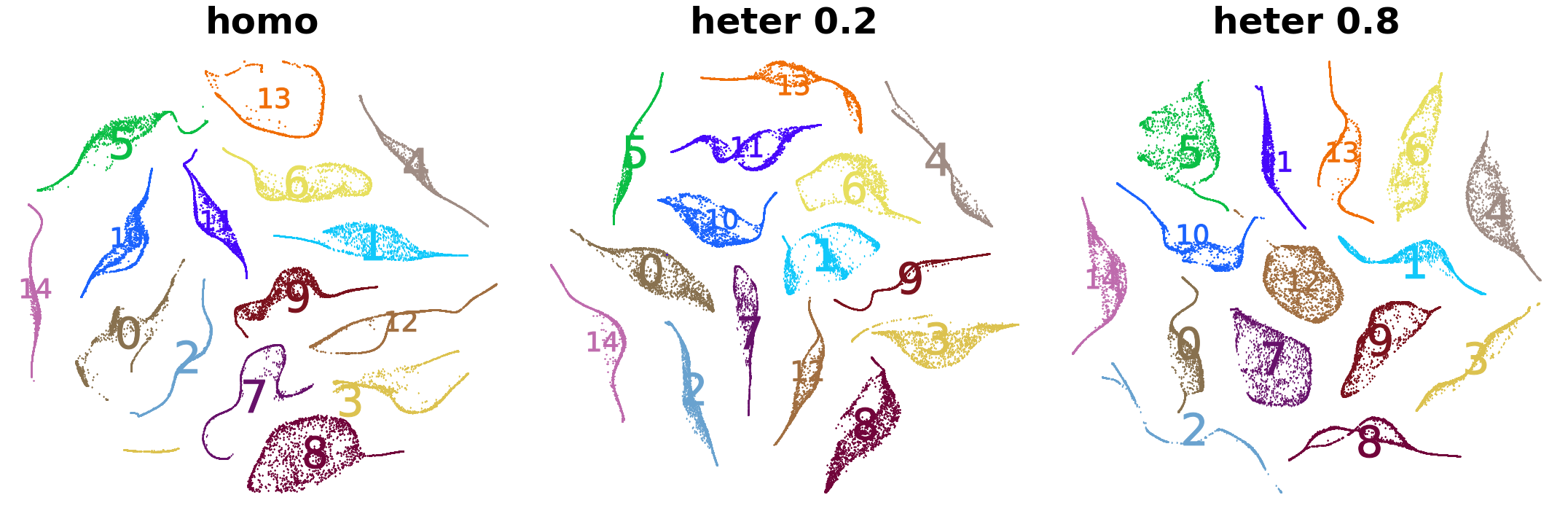
(a) Adaptiope @ 15 total clients

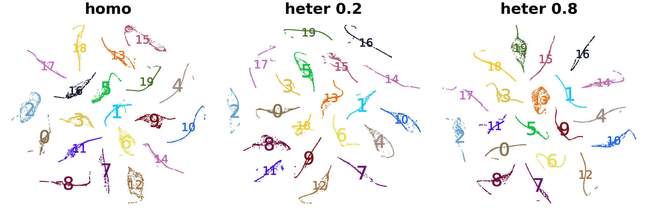
(b) Office Home @ 20 total clients

Figure 4: t-SNE of extracted style feature distributions.

Style extraction time To investigate the effect of the style extraction time, we run experiments on Adaptiope @ 1 client with $E_{s}=\{0,10,100\}$. When $E_{s}=0$, there is only biased noise infused with the content feature. Though this allows the content model to be robust to biased noise in the latent space, there is an improvement when the trained style feature is infused instead of biased noise. Figure on the right shows such improvement when style extraction time increases to 10 and 100 epochs. For SimCLR, prolonging the style extraction time too long only improves the performance slightly. For SimSiam, increasing style extraction time to 100 epochs results in better performance. But the downside of continuing style extraction for a long period is that it drastically increases the computational requirement for each client.

Local style-infused loss strength To investigate the effect of the strength of the style-infused loss on the learned representations, we run experiments with $\lambda=\{0.01,0.10,0.50,1.00,5.00,10.0\}$. We report average linear evaluations on Office Home @ 1 client and Adaptiope @ 1 client in Table 4. For the SimCLR method, as $\lambda$ is too large, personalizing with the generator $G$ fails and collapses due to the weak architecture regularization. In the case of Simsiam, both personalization and generalization deliver much lower accuracy when large $\lambda$ is applied. Simsiam still works to some extent under large $\lambda$ because it regularizes the output entropy of the model via stop-gradient operation while SimCLR only relies on architectural regularization.

	Office Home SimCLR @1 Client		Adaptiope SimSiam @ 1 Client
$\lambda$	Generalization Avg.	Personalization Avg.	Generalization Avg.	Personalization Avg.
0.01	0.542	0.518	0.634	0.647
0.10	0.540	0.512	0.635	0.649
0.50	0.549	0.535	0.639	0.651
1.00	0.546	0.354	0.624	0.638
5.00	0.539	0.022	0.542	0.566
10.0	0.534	0.021	0.552	0.566

Table 4: Effect of $\lambda$ on representations.

Conclusion

In this paper, we propose FedStyle to address the generalization of the global model and personalization of the local models in a user-centered decentralized system with unlabeled data. We propose to extract local style information to improve the global generalization and stylize the content feature to encourage local personalization. We provide an analysis of the effectiveness of style infusion in enhancing the robustness of the learned representation. The proposed method extends to multiple contrastive learning frameworks. In various controlled decentralized settings, FedStyle addresses data heterogeneity caused by heterogeneous user preference and styles.

Appendix A Information on datasets

We run experiments on the three data types. Each data type consists of different styles of same objects. This simulates the distinctive user style in a distributed system. The detail of each data type is listed in the Table 5. To sample equal number of images for each style dataset in a data type, the average number of total training images in all style datasets is sampled (duplicate sampling if necessary).

Data types	Style datasets	# object classes	# images
Digit	MNIST/SVHN/USPS	10	70k/$\sim$100k/$\sim$10k
Office Home	Art/Clipart/Product/Real World	65	$\sim$24k/$\sim$44k/$\sim$44k/$\sim$44k
Adaptiope	Sythetic/Product/Real Life	123	12.3k/12.3k/12.3k

Table 5: Dataset information

Appendix B Non-IID sampling

To sample different proportions of object classes in each client, we use a Dirichlet distribution with concentration $\beta$ to determine the number of each class to be sampled. A larger $\beta$ means a more even distribution among classes. Figure 5 shows examples of data distributions with different concentrations for different data types.

(a) Office Home 5 clients in each style, $\beta=0.2$

(b) Office Home 5 clients in each style, $\beta=0.8$

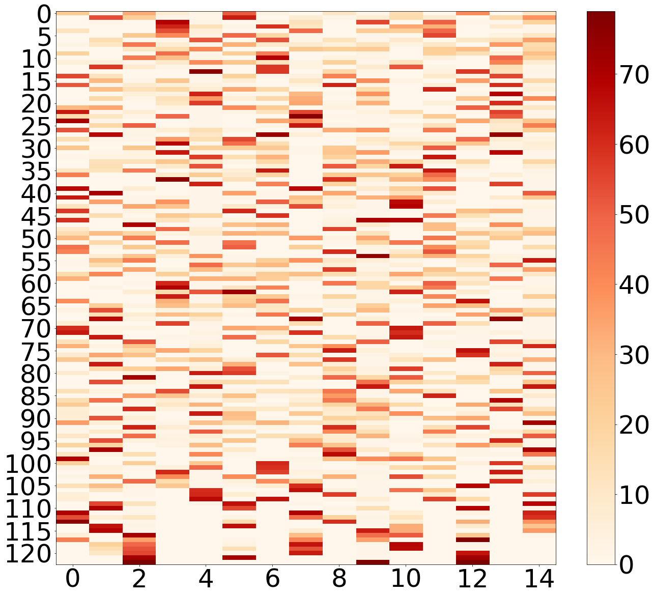
(c) Adaptiope 5 clients in each style, $\beta=0.2$

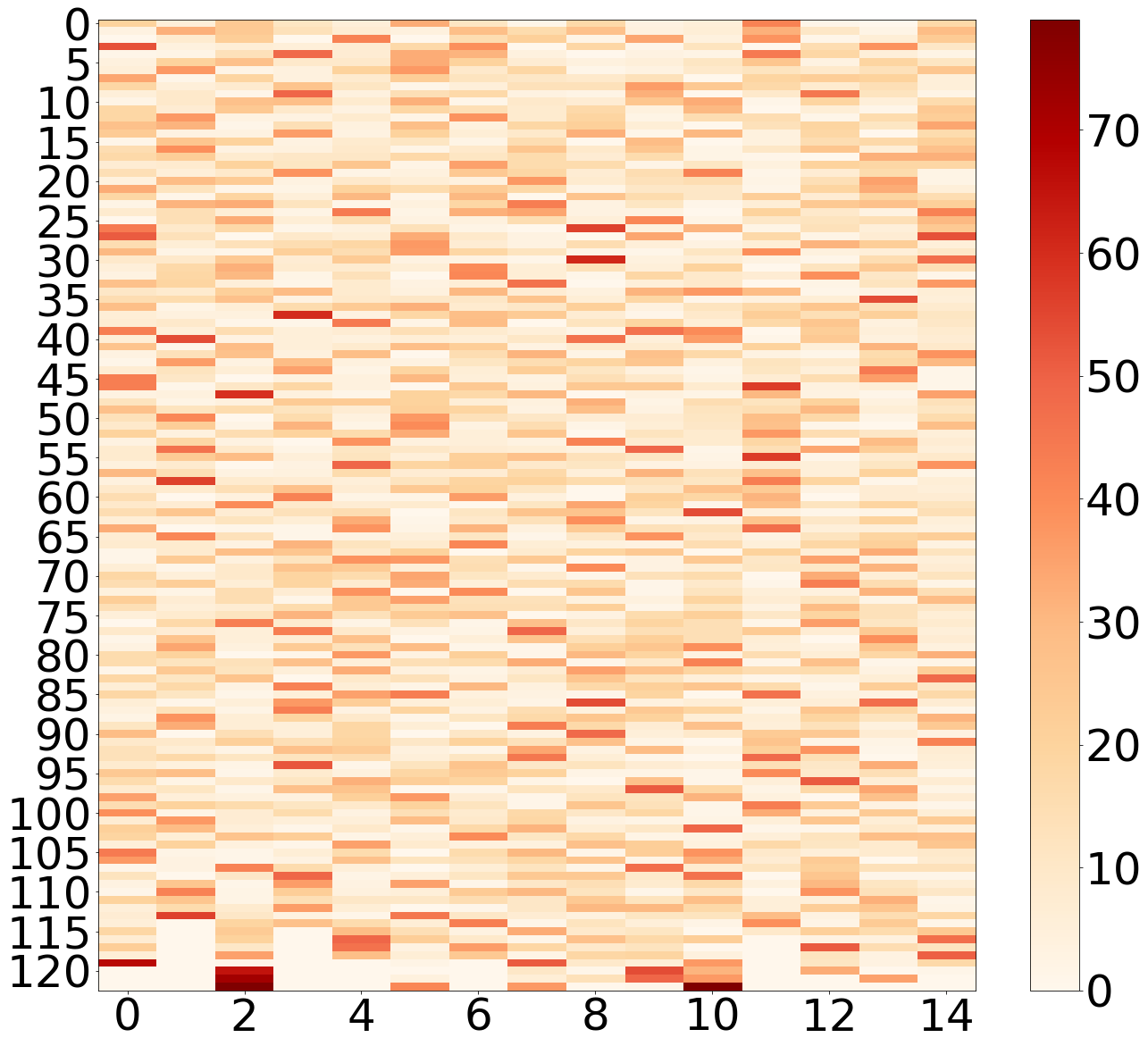
(d) Adaptiope 5 clients in each style, $\beta=0.8$

(e) Digit 10 clients in each style, $\beta=0.2$

(f) Digit 10 clients in each style, $\beta=0.8$

Figure 5: The data distribution of each client using non-IID data partition. The color bar denotes the number of data samples. Each rectangle represents the number of data samples of a specific class in a client.

Appendix C Adapting personalized methods for federated unsupervised representation learning

We adapt all baseline methods (FedAvg, FedProx, FedRep, Fedper, APFL, and Ditto) to the federated unsupervised learning since these methods are originally proposed to solve supervised problems. The workflow for all methods is as illustrated in Algorithm 1, but details in $args$, $LocalUpdate()$, and $LocalTraining$ are different and will be described in the following sections. Note that $w$ consists of weights in a feature extraction model $f$ and weights in a feature projector $g$. The default settings for parameters used in the experiments is listed in the [$args:$] for each method. lllllllllllllllllllllll lllll lll lll

ll

$LocalUpdate_{*}(w,w_{k})$

FedAvg

1:$w_{k}\leftarrow{w}$

FedRep, FedPer

1:$w^{*}_{k}\leftarrow{w^{*}}$ for $*\in{f}$

FedProx, APFL, Ditto

1:$w_{k,g}\leftarrow{w}$ // Store $w$ temporally as $w_{k,g}$

$LocalTraining_{*}(w_{k},\mathcal{D}_{k},args_{*})$

FedAvg, FedPer [$args$: None]

1:Initialize optimizer

2:for $\mathbf{x}_{\mathcal{B}}\sim{\mathcal{D}_{k}}$ do

3:   for $\mathbf{x}_{i}\sim\mathbf{x}_{\mathcal{B}}$ do

4:      $\mathbf{x}_{i}^{1},\mathbf{x}_{i}^{2}\leftarrow{Augmentations(\mathbf{x}_{i})}$

5:      $\mathbf{h}_{i}^{1}\leftarrow{f_{w_{k}}(\mathbf{x}_{i}^{1})},\mathbf{h}_{i}^{2}\leftarrow{f_{w_{k}}(\mathbf{x}_{i}^{2})}$

6:      $\mathbf{z}_{i}^{1}\leftarrow{g_{w_{k}}(\mathbf{h}_{i}^{1})},\mathbf{z}_{i}^{2}\leftarrow{g_{w_{k}}(\mathbf{h}_{i}^{2})}$

7:   end for

8:   $w_{k}\leftarrow{backward(\mathcal{L}_{unsup}(\mathbf{z}_{\mathcal{B}}^{1},\mathbf{z}_{\mathcal{B}}^{2}))}$

9:end for

FedRep [$args$:None]

1:for $epoch=1:E_{l}$ do

2:   Initialize optimizer, freeze $f_{w_{k}}$

3:   for $\mathbf{x}_{\mathcal{B}}\sim{\mathcal{D}_{k}}$ do

4:      for $\mathbf{x}_{i}\sim\mathbf{x}_{\mathcal{B}}$ do

5:         $\mathbf{x}_{i}^{1},\mathbf{x}_{i}^{2}\leftarrow{Augmentations(\mathbf{x}_{i})}$

6:         $\mathbf{h}_{i}^{1}\leftarrow{f_{w_{k}}(\mathbf{x}_{i}^{1})},\mathbf{h}_{i}^{2}\leftarrow{f_{w_{k}}(\mathbf{x}_{i}^{2})}$

7:         $\mathbf{z}_{i}^{1}\leftarrow{g_{w_{k}}(\mathbf{h}_{i}^{1})},\mathbf{z}_{i}^{2}\leftarrow{g_{w_{k}}(\mathbf{h}_{i}^{2})}$

8:      end for

9:      $g_{w_{k}}\leftarrow{backward(\mathcal{L}_{unsup}(\mathbf{z}_{\mathcal{B}}^{1},\mathbf{z}_{\mathcal{B}}^{2}))}$

10:   end for

11:end for

12:for $epoch=1:E_{l}$ do

13:   Initialize optimizer, freeze $g_{w_{k}}$

14:   for $\mathbf{x}_{\mathcal{B}}\sim{\mathcal{D}_{k}}$ do

15:      Repeat 4-8.

16:      $f_{w_{k}}\leftarrow{backward(\mathcal{L}_{unsup}(\mathbf{z}_{\mathcal{B}}^{1},\mathbf{z}_{\mathcal{B}}^{2}))}$

17:   end for

18:end for

APFL [$args:\alpha=0.5,w_{k,g}$]

1:Initialize optimizers

2:for $\mathbf{x}_{\mathcal{B}}\sim{\mathcal{D}_{k}}$ do

3:   for $\mathbf{x}_{i}\sim\mathbf{x}_{\mathcal{B}}$ do

4:      $\mathbf{x}_{i}^{1},\mathbf{x}_{i}^{2}\leftarrow{Augmentations(\mathbf{x}_{i})}$

5:      $\mathbf{h}_{i,g}^{1}\leftarrow{f_{w_{k,g}}(\mathbf{x}_{i}^{1})},\mathbf{h}_{i,g}^{2}\leftarrow{f_{w_{k,g}}(\mathbf{x}_{i}^{2})}$

6:      $\mathbf{z}_{i,g}^{1}\leftarrow{g_{w_{k,g}}(\mathbf{h}_{i,g}^{1})},\mathbf{z}_{i,g}^{2}\leftarrow{g_{w_{k,g}}(\mathbf{h}_{i,g}^{2})}$

7:      $\mathbf{h}_{i}^{1}\leftarrow{f_{w_{k}}(\mathbf{x}_{i}^{1})},\mathbf{h}_{i}^{2}\leftarrow{f_{w_{k}}(\mathbf{x}_{i}^{2})}$

8:      $\mathbf{z}_{i}^{1}\leftarrow{g_{w_{k}}(\mathbf{h}_{i}^{1})},\mathbf{z}_{i}^{2}\leftarrow{g_{w_{k}}(\mathbf{h}_{i}^{2})}$

9:      $\mathbf{\hat{z}}_{i}^{1}\leftarrow{\alpha\times{\mathbf{z}^{1}_{i,g}.detach()}+(1-\alpha)\times{\mathbf{z}_{i}^{2}}}$

10:      $\mathbf{\hat{z}}_{i}^{2}\leftarrow{\alpha\times{\mathbf{z}^{2}_{i,g}.detach()}+(1-\alpha)\times{\mathbf{z}_{i}^{2}}}$

11:   end for

12:   $w_{k,g}\leftarrow{backward(\mathcal{L}_{unsup}(\mathbf{z}_{\mathcal{B}}^{1},\mathbf{z}_{\mathcal{B}}^{2}))}$

13:   $w_{k}\leftarrow{backward(\mathcal{L}_{unsup}(\mathbf{\hat{z}}_{\mathcal{B}}^{1},\mathbf{\hat{z}}_{\mathcal{B}}^{2}))}$

14:end for

FedProx [$args:\mu=0.2,w_{k,g}$]

1:Initialize optimizer

2:for $\mathbf{x}_{\mathcal{B}}\sim{\mathcal{D}_{k}}$ do

3:   for $\mathbf{x}_{i}\sim\mathbf{x}_{\mathcal{B}}$ do

4:      $\mathbf{x}_{i}^{1},\mathbf{x}_{i}^{2}\leftarrow{Augmentations(\mathbf{x}_{i})}$

5:      $\mathbf{h}_{i}^{1}\leftarrow{f_{w_{k}}(\mathbf{x}_{i}^{1})},\mathbf{h}_{i}^{2}\leftarrow{f_{w_{k}}(\mathbf{x}_{i}^{2})}$

6:      $\mathbf{z}_{i}^{1}\leftarrow{g_{w_{k}}(\mathbf{h}_{i}^{1})},\mathbf{z}_{i}^{2}\leftarrow{g_{w_{k}}(\mathbf{h}_{i}^{2})}$

7:   end for

8:   $w_{k}\leftarrow{backward(\mathcal{L}_{unsup}(\mathbf{z}_{\mathcal{B}}^{1},\mathbf{z}_{\mathcal{B}}^{2})+\frac{\mu}{2}||w_{k}-w_{k,g}||^{2})}$

9:end for

Ditto [$args:\mu=2,w_{k,g}$]

1:for $epoch=1:E_{l}$ do

2:   Initialize optimizer

3:   for $\mathbf{x}_{\mathcal{B}}\sim{\mathcal{D}_{k}}$ do

4:      for $\mathbf{x}_{i}\sim\mathbf{x}_{\mathcal{B}}$ do

5:         $\mathbf{x}_{i}^{1},\mathbf{x}_{i}^{2}\leftarrow{Augmentations(\mathbf{x}_{i})}$

6:         $\mathbf{h}_{i,g}^{1}\leftarrow{f_{w_{k,g}}(\mathbf{x}_{i}^{1})},\mathbf{h}_{i,g}^{2}\leftarrow{f_{w_{k,g}}(\mathbf{x}_{i}^{2})}$

7:         $\mathbf{z}_{i,g}^{1}\leftarrow{g_{w_{k,g}}(\mathbf{h}_{i,g}^{1})},\mathbf{z}_{i,g}^{2}\leftarrow{g_{w_{k,g}}(\mathbf{h}_{i,g}^{2})}$

8:      end for

9:      $w_{k,g}\leftarrow{backward(\mathcal{L}_{unsup}(\mathbf{z}_{\mathcal{B},g}^{1},\mathbf{z}_{\mathcal{B},g}^{2}))}$

10:   end for

11:end for

12:for $epoch=1:E_{l}$ do

13:   Initialize optimizer

14:   for $\mathbf{x}_{\mathcal{B}}\sim{\mathcal{D}_{k}}$ do

15:      for $\mathbf{x}_{i}\sim\mathbf{x}_{\mathcal{B}}$ do

16:         $\mathbf{x}_{i}^{1},\mathbf{x}_{i}^{2}\leftarrow{Augmentations(\mathbf{x}_{i})}$

17:         $\mathbf{h}_{i}^{1}\leftarrow{f_{w_{k}}(\mathbf{x}_{i}^{1})},\mathbf{h}_{i}^{2}\leftarrow{f_{w_{k}}(\mathbf{x}_{i}^{2})}$

18:         $\mathbf{z}_{i}^{1}\leftarrow{g_{w_{k}}(\mathbf{h}_{i}^{1})},\mathbf{z}_{i}^{2}\leftarrow{g_{w_{k}}(\mathbf{h}_{i}^{2})}$

19:      end for

20:      $\begin{aligned} w_{k}\leftarrow backward(\mathcal{L}_{unsup}(&\mathbf{z}_{\mathcal{B}}^{1},\mathbf{z}_{\mathcal{B}}^{2})\\ &+\frac{\mu}{2}||w_{k}-w_{k,g}||^{2})\end{aligned}$

21:   end for

22:end for

References

- Arivazhagan et al. (2019) Arivazhagan, M. G.; Aggarwal, V.; Singh, A. K.; and Choudhary, S. 2019. Federated learning with personalization layers. arXiv preprint arXiv:1912.00818.
- Briggs, Fan, and Andras (2020) Briggs, C.; Fan, Z.; and Andras, P. 2020. Federated learning with hierarchical clustering of local updates to improve training on non-IID data. In 2020 International Joint Conference on Neural Networks (IJCNN), 1–9. IEEE.
- Chen et al. (2020a) Chen, T.; Kornblith, S.; Norouzi, M.; and Hinton, G. 2020a. A simple framework for contrastive learning of visual representations. In International conference on machine learning, 1597–1607. PMLR.
- Chen et al. (2020b) Chen, X.; Fan, H.; Girshick, R.; and He, K. 2020b. Improved baselines with momentum contrastive learning. arXiv preprint arXiv:2003.04297.
- Chen and He (2021) Chen, X.; and He, K. 2021. Exploring simple siamese representation learning. In Proceedings of the IEEE/CVF Conference on Computer Vision and Pattern Recognition, 15750–15758.
- Collins et al. (2021) Collins, L.; Hassani, H.; Mokhtari, A.; and Shakkottai, S. 2021. Exploiting shared representations for personalized federated learning. In International Conference on Machine Learning, 2089–2099. PMLR.
- Deng (2012) Deng, L. 2012. The mnist database of handwritten digit images for machine learning research. IEEE Signal Processing Magazine, 29(6): 141–142.
- Deng, Kamani, and Mahdavi (2020) Deng, Y.; Kamani, M. M.; and Mahdavi, M. 2020. Adaptive personalized federated learning. arXiv preprint arXiv:2003.13461.
- Dinh et al. (2021) Dinh, C. T.; Vu, T. T.; Tran, N. H.; Dao, M. N.; and Zhang, H. 2021. Fedu: A unified framework for federated multi-task learning with laplacian regularization. arXiv preprint arXiv:2102.07148.
- Donahue and Simonyan (2019) Donahue, J.; and Simonyan, K. 2019. Large scale adversarial representation learning. Advances in neural information processing systems, 32.
- Fallah, Mokhtari, and Ozdaglar (2020) Fallah, A.; Mokhtari, A.; and Ozdaglar, A. 2020. Personalized federated learning with theoretical guarantees: A model-agnostic meta-learning approach. Advances in Neural Information Processing Systems, 33: 3557–3568.
- Fetterman and Albrecht (2020) Fetterman, A.; and Albrecht, J. 2020. Understanding self-supervised and contrastive learning with bootstrap your own latent (BYOL). Untitled AI, August.
- Gidaris, Singh, and Komodakis (2018) Gidaris, S.; Singh, P.; and Komodakis, N. 2018. Unsupervised representation learning by predicting image rotations. arXiv preprint arXiv:1803.07728.
- Grill et al. (2020) Grill, J.-B.; Strub, F.; Altché, F.; Tallec, C.; Richemond, P.; Buchatskaya, E.; Doersch, C.; Avila Pires, B.; Guo, Z.; Gheshlaghi Azar, M.; et al. 2020. Bootstrap your own latent-a new approach to self-supervised learning. Advances in neural information processing systems, 33: 21271–21284.
- Haykin (1994) Haykin, S. 1994. Neural networks: a comprehensive foundation. Prentice Hall PTR.
- He et al. (2021) He, C.; Yang, Z.; Mushtaq, E.; Lee, S.; Soltanolkotabi, M.; and Avestimehr, S. 2021. Ssfl: Tackling label deficiency in federated learning via personalized self-supervision. arXiv preprint arXiv:2110.02470.
- He et al. (2022) He, K.; Chen, X.; Xie, S.; Li, Y.; Dollár, P.; and Girshick, R. 2022. Masked autoencoders are scalable vision learners. In Proceedings of the IEEE/CVF Conference on Computer Vision and Pattern Recognition, 16000–16009.
- He et al. (2016) He, K.; Zhang, X.; Ren, S.; and Sun, J. 2016. Deep residual learning for image recognition. In Proceedings of the IEEE conference on computer vision and pattern recognition, 770–778.
- Hull (1994) Hull, J. J. 1994. A database for handwritten text recognition research. IEEE Transactions on Pattern Analysis and Machine Intelligence, 16(5): 550–554.
- Jaiswal et al. (2020) Jaiswal, A.; Babu, A. R.; Zadeh, M. Z.; Banerjee, D.; and Makedon, F. 2020. A survey on contrastive self-supervised learning. Technologies, 9(1): 2.
- Kanopoulos, Vasanthavada, and Baker (1988) Kanopoulos, N.; Vasanthavada, N.; and Baker, R. L. 1988. Design of an image edge detection filter using the Sobel operator. IEEE Journal of solid-state circuits, 23(2): 358–367.
- Khodak, Balcan, and Talwalkar (2019) Khodak, M.; Balcan, M.-F. F.; and Talwalkar, A. S. 2019. Adaptive gradient-based meta-learning methods. Advances in Neural Information Processing Systems, 32.
- Li et al. (2021) Li, T.; Hu, S.; Beirami, A.; and Smith, V. 2021. Ditto: Fair and robust federated learning through personalization. In International Conference on Machine Learning, 6357–6368. PMLR.
- Li et al. (2020) Li, T.; Sahu, A. K.; Zaheer, M.; Sanjabi, M.; Talwalkar, A.; and Smith, V. 2020. Federated optimization in heterogeneous networks. Proceedings of Machine Learning and Systems, 2: 429–450.
- Li et al. (2019) Li, W.; Milletarì, F.; Xu, D.; Rieke, N.; Hancox, J.; Zhu, W.; Baust, M.; Cheng, Y.; Ourselin, S.; Cardoso, M. J.; et al. 2019. Privacy-preserving federated brain tumour segmentation. In International workshop on machine learning in medical imaging, 133–141. Springer.
- Liu et al. (2020) Liu, Y.; Huang, A.; Luo, Y.; Huang, H.; Liu, Y.; Chen, Y.; Feng, L.; Chen, T.; Yu, H.; and Yang, Q. 2020. Fedvision: An online visual object detection platform powered by federated learning. In Proceedings of the AAAI Conference on Artificial Intelligence, volume 34, 13172–13179.
- Long, Shelhamer, and Darrell (2015) Long, J.; Shelhamer, E.; and Darrell, T. 2015. Fully convolutional networks for semantic segmentation. In Proceedings of the IEEE conference on computer vision and pattern recognition, 3431–3440.
- Marfoq et al. (2021) Marfoq, O.; Neglia, G.; Bellet, A.; Kameni, L.; and Vidal, R. 2021. Federated multi-task learning under a mixture of distributions. Advances in Neural Information Processing Systems, 34: 15434–15447.
- McMahan et al. (2017) McMahan, B.; Moore, E.; Ramage, D.; Hampson, S.; and y Arcas, B. A. 2017. Communication-efficient learning of deep networks from decentralized data. In Artificial intelligence and statistics, 1273–1282. PMLR.
- Mohsenvand, Izadi, and Maes (2020) Mohsenvand, M. N.; Izadi, M. R.; and Maes, P. 2020. Contrastive representation learning for electroencephalogram classification. In Machine Learning for Health, 238–253. PMLR.
- Netzer et al. (2011) Netzer, Y.; Wang, T.; Coates, A.; Bissacco, A.; Wu, B.; and Ng, A. Y. 2011. Reading digits in natural images with unsupervised feature learning.
- Noroozi and Favaro (2016) Noroozi, M.; and Favaro, P. 2016. Unsupervised learning of visual representations by solving jigsaw puzzles. In European conference on computer vision, 69–84. Springer.
- Oord, Li, and Vinyals (2018) Oord, A. v. d.; Li, Y.; and Vinyals, O. 2018. Representation learning with contrastive predictive coding. arXiv preprint arXiv:1807.03748.
- Ringwald and Stiefelhagen (2021) Ringwald, T.; and Stiefelhagen, R. 2021. Adaptiope: A Modern Benchmark for Unsupervised Domain Adaptation. In Proceedings of the IEEE/CVF Winter Conference on Applications of Computer Vision (WACV), 101–110.
- Saeed, Grangier, and Zeghidour (2021) Saeed, A.; Grangier, D.; and Zeghidour, N. 2021. Contrastive learning of general-purpose audio representations. In ICASSP 2021-2021 IEEE International Conference on Acoustics, Speech and Signal Processing (ICASSP), 3875–3879. IEEE.
- Sattler, Müller, and Samek (2020) Sattler, F.; Müller, K.-R.; and Samek, W. 2020. Clustered federated learning: Model-agnostic distributed multitask optimization under privacy constraints. IEEE transactions on neural networks and learning systems, 32(8): 3710–3722.
- Tschannen et al. (2019) Tschannen, M.; Djolonga, J.; Rubenstein, P. K.; Gelly, S.; and Lucic, M. 2019. On mutual information maximization for representation learning. arXiv preprint arXiv:1907.13625.
- Van der Maaten and Hinton (2008) Van der Maaten, L.; and Hinton, G. 2008. Visualizing data using t-SNE. Journal of machine learning research, 9(11).
- Venkateswara et al. (2017) Venkateswara, H.; Eusebio, J.; Chakraborty, S.; and Panchanathan, S. 2017. Deep hashing network for unsupervised domain adaptation. In Proceedings of the IEEE Conference on Computer Vision and Pattern Recognition, 5018–5027.
- Von Kügelgen et al. (2021) Von Kügelgen, J.; Sharma, Y.; Gresele, L.; Brendel, W.; Schölkopf, B.; Besserve, M.; and Locatello, F. 2021. Self-supervised learning with data augmentations provably isolates content from style. Advances in neural information processing systems, 34: 16451–16467.
- Wu et al. (2021) Wu, Y.; Wang, Z.; Zeng, D.; Li, M.; Shi, Y.; and Hu, J. 2021. Federated Contrastive Representation Learning with Feature Fusion and Neighborhood Matching.
- Zbontar et al. (2021) Zbontar, J.; Jing, L.; Misra, I.; LeCun, Y.; and Deny, S. 2021. Barlow twins: Self-supervised learning via redundancy reduction. In International Conference on Machine Learning, 12310–12320. PMLR.
- Zhang et al. (2020) Zhang, F.; Kuang, K.; You, Z.; Shen, T.; Xiao, J.; Zhang, Y.; Wu, C.; Zhuang, Y.; and Li, X. 2020. Federated unsupervised representation learning. arXiv preprint arXiv:2010.08982.
- Zhang, Isola, and Efros (2016) Zhang, R.; Isola, P.; and Efros, A. A. 2016. Colorful image colorization. In European conference on computer vision, 649–666. Springer.
- Zhuang et al. (2021) Zhuang, W.; Gan, X.; Wen, Y.; Zhang, S.; and Yi, S. 2021. Collaborative unsupervised visual representation learning from decentralized data. In Proceedings of the IEEE/CVF International Conference on Computer Vision, 4912–4921.