Anomalies and the Green-Schwarz Mechanism

Abstract

Anomalies are a very powerful tool in constraining theories beyond the standard model. We give a pedagogical overview of some topics illustrating the important role played by spacetime anomalies in string theory. After discussing the general problem of anomaly cancellation in quantum field theory, the focus is set on the cancellation of anomalies in type-I string theory through the Green-Schwarz mechanism. The notion of anomaly inflow is also reviewed, as well as its application to the evaluation of D-brane anomalous couplings. Finally, we briefly comment on recent developments concerning the reformulation of anomalies in the language of category theory.

1 The trouble with anomalies

To the best of our knowledge, all fundamental interactions in nature are carried by quantum fields of spin one and two. Unlike scalar or spinors, the quantization of these fields requires special care in order to preserve locality and Lorentz invariance. A way to achieve this is by introducing redundant degrees of freedom living in an extended Hilbert space $\mathcal{H}$, so physical states are represented by equivalence classes under the action of a group $\mathcal{G}$. The freedom to switch from one representative to another without changing the physics is what we call gauge invariance, and the space of physical states is obtained as the quotient $\mathcal{H}_{\rm phys}\equiv\mathcal{H}/\mathcal{G}$ QFT_book . Unlike standard physical symmetries mapping one state of the physical Hilbert space into another, gauge invariance only changes the state representative, the label so to speak, acting thus trivially on $\mathcal{H}_{\rm phys}$.

For this to work it is crucial to preserve the invariance under the choice of representative. Otherwise, spurious states in $\mathcal{H}$ would enter $\mathcal{H}_{\rm phys}$ rendering the theory nonunitary. This may occur in chiral theories of the type of the standard model (SM), where gauge invariance can be broken in the process of quantization due to the necessary regularization. Whenever this happens, the theory is said to be anomalous QFT_book ; anomalies_rev ; harvey_review . The requirement of chirality implies that gauge anomalies can only arise when the spacetime dimension is even.

Characterizing anomalies in gauge theories is thus of the utmost importance and its mandatory cancellation poses very strict constraints on both the theory’s spectrum and interactions. The SM is a glaring example of this: the condition that all gauge and mixed gauge-gravitational anomalies cancel leads to an essentially complete determination of hypercharges, up to a global normalization. In the minimal supersymmetric standard model (MSSM), on the other hand, the introduction of an additional Higgs doublet is necessary in order to cancel the anomaly induced by the chiral higgsino (see pages 3-3).

At a diagrammatic level, anomalies are signaled by violations of the gauge Ward identities induced by the parity-violating part of one-loop diagrams with gauge current insertions and chiral fields running in the loop. In the case of the SM or their supersymmetric extensions the relevant fields are the chiral fermions but, as we will see later, higher-dimensional theories also contain bosonic fields contributing to the anomaly. On general grounds, in $D=2n-2$ spacetime dimensions the anomaly is determined by a one-loop diagram with $n$ current insertions, which in four dimensions gives the celebrated triangle diagram. One-loop diagrams with more than $n$ currents also contribute to the anomaly in non-Abelian theories, but their values are fully determined by the $n$-point diagram, so one only needs to cancel the latter.

Functional methods offer a very powerful alternative to the diagrammatic analysis of anomalies. The basic object to consider is the effective action $\Gamma_{\rm eff}$, obtained by integrating out all chiral degrees of freedom in the theory. Since these are massless fields, $\Gamma_{\rm eff}$ is a nonlocal functional resumming all one-loop diagrams with an arbitrary number of gauge current insertions.

Up to now, we have been talking about anomalies affecting any sort of gauge invariance, although they come in various kinds. It is however necessary to be more specific and distinguish among different types. First, we have gauge (consistent) anomalies, associated with the noninvariance of the effective action under infinitesimal gauge transformations $\delta_{\chi}\mathcal{A}_{\mu}=\partial_{\mu}\chi+[\mathcal{A}_{\mu},\chi]$

$$\delta_{\chi}\Gamma_{\rm eff}\neq 0.$$ (1)

Their presence leads to quantum violations of the conservation of the corresponding gauge current. For theories coupled to gravity, on the other hand, anomalies can also spoil the covariant conservation of the expectation value of the energy-momentum tensor, $\nabla_{\mu}\langle T^{\mu\nu}\rangle\neq 0$. These are called Einstein anomalies and are associated with the effective action’s noninvariance with respect to infinitesimal diffeomorphisms

$$\delta_{\rm diff}\Gamma_{\rm eff}\neq 0.$$ (2)

General relativity can also be understood as a gauge theory of local frame rotations, $e^{a}_{\,\,\,\mu}\rightarrow\Lambda^{a}_{\,\,\,b}e^{b}_{\,\,\,\mu}$, where $\Lambda^{a}_{\,\,\,b}$ is a Lorentz transformations and $e^{a}_{\,\,\,\mu}$ is the vielbein. This invariance can also be anomalous if gravity couples to chiral fields, giving rise to so-called Lorentz anomalies. They are signalled by a nonzero variation of the effective action under infinitesimal local Lorentz transformations $\Lambda=\mathbb{1}+\epsilon$

$$\delta_{\epsilon}\Gamma_{\rm eff}\neq 0.$$ (3)

In fact, it is always possible to find a local counterterm that added to the effective action shifts Lorentz into Einstein anomalies and vice versa BZ_NPB ; AG_GinspargAP . We will take this into account and focus our attention on Lorentz anomalies from now on.

In this chapter of the Handbook we do not enter into a detailed discussion of quantum field theory anomalies, a subject that is surveyed in a number of books and reviews (see, for instance, anomalies_rev ; harvey_review ). Instead, we limit our general presentation of anomalies to the basic recipes necessary to address the problem of their cancellation, with a focus on the role played by this requirement in string theory. To this aim, two particular topics are selected. First, we carry out a detailed analysis of the workings of the Green-Schwarz (GS) mechanism, which was of pivotal importance in the development of string theory and goes well beyond the ten-dimensional open superstring theory in which it was first uncovered. Next, we study the seminal notion of anomaly inflow. To illustrate its implementation, we review how anomalous D-brane (and orientifold) couplings are determined by the condition that worldvolume anomalies are cancelled by charge accretion/depletion. Our overview will be closed by a very brief discussion on the modern understanding of anomalies, that has led to a suggestive connection with category theory.

2 Anomaly polynomials and Chern-Simons forms

The main advantage of the effective action approach is that the anomaly can be computed from very general geometrical and topological considerations. It might be puzzling that this is possible at all, given the fact that anomalies are usually seen as the result of UV ambiguities in the calculation of the Ward-Takahashi identities. This being true, anomalies can also be interpreted as stemming from IR effects, signaled by zero-momentum poles in the expectation value of the anomalous currents themselves. It is this IR side of anomalies that makes it possible that they can be captured by studying the topological properties of the vector bundles associated with the gauge and gravitational theories nakahara .

As a general rule, anomalies on a $D$-dimensional curved manifold are determined by an anomaly polynomial in $D+2=2n$ dimensions zumino , constructed from traces of powers of the spacetime curvature and the gauge field strength

$$I_{2n}=P({\rm Tr\,}\mathcal{R}^{2},\ldots,{\rm Tr\,}\mathcal{R}^{n};{\rm tr\,}\mathcal{F},\ldots,{\rm tr\,}\mathcal{F}^{n}).$$ (4)

Here $\mathcal{R}$ denotes the curvature two-form $\mathcal{R}^{a}_{\,\,\,b}=d\omega^{a}_{\,\,\,b}+\omega^{a}_{\,\,\,c}\omega^{c}_{\,\,\,b}$ (with $\omega^{a}_{\,\,b}$ the spin connection) and $\mathcal{F}$ is the gauge field strength, defined from the gauge potential $\mathcal{A}$ by $\mathcal{F}=d\mathcal{A}+\mathcal{A}^{2}$. In addition, “${\rm Tr\,}$” and “${\rm tr\,}$” respectively represent trace over Lorentz and gauge indices in the appropriate representation. Expression (4) shows that the anomaly polynomial is invariant under local frame rotations and gauge transformations

$$\mathcal{R}^{a}_{\,\,\,b} \longrightarrow\Lambda^{a}_{\,\,\,\,c}\mathcal{R}^{c}_{\,\,\,d}(\Lambda^{T})^{d}_{\,\,\,\,b},$$

$$\mathcal{F} \longrightarrow g^{-1}\mathcal{F}g,$$ (5)

with $\Lambda^{a}_{\,\,\,\,b}\in\mbox{SO(1,$D-1$)}$ and $g\in\mathcal{G}$, the Lorentz and gauge groups respectively. By the index theorem, the integrated anomaly polynomial equals the index of certain differential operator in $D+2$ dimensions AG_GinspargNPB ; AG_GinspargAP ; AG_Witten .

Equation (4) also shows that the anomaly polynomial $I_{2n}$ is a closed differential form, $dI_{2n}=0$. In fact, by Poincaré’s lemma, it is also locally exact

$$I_{2n}=dI^{0}_{2n-1},$$ (6)

where $I^{0}_{2n-1}$ is the Chern-Simons form. This $(2n-1)$-form can be integrated over a $(2n-1)$-dimensional manifold $\mathcal{M}_{2n-1}$, whose boundary $\partial\mathcal{M}_{2n-1}$ is identified with the physical (Euclidean) spacetime. The result gives all the terms of the one-loop quantum effective action associated with the anomaly

$$\Gamma_{\rm eff}=2\pi i\int_{\mathcal{M}_{2n-1}}I^{0}_{2n-1}.$$ (7)

The global normalization of the integral is determined by either the index theorem or the diagrammatic calculation. From the point of view of the $(2n-2)$-dimensional physical spacetime the action (7) is nonlocal. This is to be expected, since $\Gamma_{\rm eff}$ results from integrating out a number of massless chiral fields. Moreover, the Chern-Simons form is not uniquely determined by eq. (6) since we are at liberty of shifting it by an arbitrary $(2n-2)$-form, $I^{0}_{2n-1}\rightarrow I^{0}_{2n-1}+d\eta_{2n-2}$, without modifying it. This ambiguity reflects the freedom to add any local counterterm to the quantum effective action. Indeed, once integrated over $\mathcal{M}_{2n-1}$ the previous shift amounts to

$$\Gamma_{\rm eff}\longrightarrow\Gamma_{\rm eff}+2\pi i\int_{\partial\mathcal{M}_{2n-1}}\eta_{2n-2},$$ (8)

where the last term, being an integral over physical space, is indeed local.

A crucial property of the Chern-Simons form is that, unlike the anomaly polynomial, it is not gauge or Lorentz invariant. It can be shown, however, that its gauge variation is a closed differential form, $d\delta I^{0}_{2n-1}=0$, and therefore is also locally exact

$$\delta I^{0}_{2n-1}=dI^{1}_{2n-2}.$$ (9)

Since we are taking infinitesimal transformations, the right-hand side is linear in the gauge functions, as indicated by the superscript of $I^{1}_{2n-2}$. The anomaly is obtained by performing a gauge variation on the effective action (7)

$$\delta\Gamma_{\rm eff}=2\pi i\int_{\partial\mathcal{M}_{2n-1}}I^{1}_{2n-2}.$$ (10)

To be precise, this gives the so-called consistent anomaly. The name implies that this form of the anomaly satisfies the Wess-Zumino consistency conditions, a consequence of the fact that the commutator of two gauge (resp. Lorentz) transformations acting on the effective action equals the action of the transformation associated with their commutator. Although the consistent anomaly is not generically gauge covariant, a covariant form of the anomaly can be obtained by redefining the gauge current and adding counterterms BZ_NPB .

3 Anomaly cancellation

The previous discussion sets the framework to analyze anomaly cancellation: for a given theory, we should find its anomaly polynomial and see whether it is zero or not. Fortunately, there are powerful mathematical theorems at our disposal leading to a direct computation of the anomaly polynomial for any kind of fields (see anomalies_rev ; nakahara ). In the case of a Weyl fermion, the Atiyah-Singer index theorem in $2n=D+2$ dimensions leads to the explicit expression

$$I_{1\over 2}=\big{[}\widehat{A}(\mathcal{M}){\rm ch}(\mathcal{F})\big{]}_{2n}.$$ (11)

The subscript on the right-hand side indicates that we retain only the $2n$-form piece of the polynomial inside the brackets, and negative chirality spinors contribute with the same polynomial and the opposite sign. The term $\widehat{A}(\mathcal{M})$ is called the $A$-roof (or Dirac) genus and is determined by the curvature two-form. To give its explicit expression, we notice that $\mathcal{R}^{a}_{\,\,\,b}$ defines a $(2n)\times(2n)$ antisymmetric matrix of two-forms that can be brought to a block skew-diagonal form by an appropriate orthogonal transformation

$${1\over 2\pi}\mathcal{R}=\left(\begin{array}[]{ccccc}0&x_{1}&&&\\ -x_{1}&0&&&\\ &&0&x_{2}&\\ &&-x_{2}&0&\\ &&&&\ddots\end{array}\right).$$ (17)

It is convenient to encode these skew eigenvalues in terms of the total Pontrjagin class

$$p(\mathcal{R})=\prod_{i=1}^{n}(1+x_{i}^{2})\equiv 1+p_{1}(\mathcal{R})+p_{2}(\mathcal{R})+\ldots+p_{n}(\mathcal{R}),$$ (18)

where the $\ell$-th Poitrjagin class is defined as the homogeneous polynomial anomalies_rev ; nakahara

$$p_{\ell}(\mathcal{R})=\sum_{i_{1}<\ldots<i_{\ell}}^{n}x_{i_{1}}^{2}\ldots x_{i_{\ell}}^{2}.$$ (19)

These are $4\ell$-forms. Noticing that

$${\rm Tr\,}\mathcal{R}^{2\ell}=(-1)^{\ell}\sum_{a=1}^{n}x_{a}^{2\ell},\hskip 28.45274pt{\rm Tr\,}\mathcal{R}^{2\ell+1}=0,$$ (20)

it is easy to write $p_{\ell}(\mathcal{R})$ in terms of traces of powers of the curvature two-form. For the first few cases to be used later, we have

$$p_{1} =-{1\over 8\pi^{2}}{\rm Tr\,}\mathcal{R}^{2},$$

$$p_{2} ={1\over 128\pi^{4}}\Big{[}\big{(}{\rm Tr\,}\mathcal{R}^{2}\big{)}^{2}-2{\rm Tr\,}\mathcal{R}^{4}\Big{]},$$ (21)

$$p_{3} =-{1\over 3072\pi^{6}}\Big{[}\big{(}{\rm Tr\,}\mathcal{R}^{2}\big{)}^{3}-6\big{(}{\rm Tr\,}\mathcal{R}^{2}\big{)}\big{(}{\rm Tr\,}\mathcal{R}^{4}\big{)}+8{\rm Tr\,}\mathcal{R}^{6}\Big{]},$$

where, to simplify expressions, we omit the dependence of $p_{k}$ on $\mathcal{R}$. Using Pontrjagin classes, the $A$-roof genus in (11) can be written as the polynomial

$$\widehat{A}(\mathcal{M}) \equiv\prod_{a=1}^{n}{x_{a}/2\over\sinh{(x_{a}/2)}}$$ (22)

$$=1-{1\over 24}p_{1}+{1\over 5760}\big{(}7p_{1}^{2}-4p_{2}\big{)}-{1\over 967680}\big{(}31p_{1}^{3}-44p_{1}p_{2}+16p_{3}\big{)}+\ldots$$

As we will soon see, Pontrjagin classes are also useful in writing the contribution of other fields to the gravitational anomaly.

The second factor on the right-hand side of eq. (11), containing all the dependence on the gauge field, is the Chern character. It is defined by the formal series

$${\rm ch}(\mathcal{F}) =\sum_{j=0}^{n}{1\over j!}{\rm tr\,}\left({i\over 2\pi}\mathcal{F}\right)^{j}$$

$$={\rm ch}_{0}(\mathcal{F})+{\rm ch}_{1}(\mathcal{F})+\ldots+{\rm ch}_{n}(\mathcal{F}),$$ (23)

with the $2j$-form

$${\rm ch}_{j}(\mathcal{F})\equiv{1\over j!}{\rm tr}_{R}\left({i\over 2\pi}\mathcal{F}\right)^{j},$$ (24)

defining the $j$-th Chern character. The subscript $R$ indicates that the traces are taken in the representation $R$ in which the fermions transform, with ${\rm ch}_{0}(\mathcal{F})=N$ its dimension. Taking the exterior product of eqs. (22) and (23) and retaining the $2n$-form piece, we get the contribution of a chiral fermion to the anomaly polynomial in any even dimension.

Both Pontrjagin classes and Chern characters are closed forms that can be written locally in terms of the corresponding gravitational and gauge Chern-Simons forms as

$$p_{\ell}(\mathcal{R})=d\Omega^{0}_{4\ell-1}(\mathcal{R},\omega),\hskip 28.45274pt{\rm ch}_{k}(\mathcal{F})=d\omega^{0}_{4k-1}(\mathcal{F},\mathcal{A}).$$ (25)

As explicitly indicated, these forms depend on the spin connection and the gauge field respectively. Unlike their parent polynomials, they are not invariant under local Lorentz and gauge transformations. Their infinitesimal variations define differential forms through the descent equations

$$\delta_{\epsilon}\Omega^{0}_{4\ell-1}(\mathcal{R},\omega) =d\Omega^{1}_{4\ell-2}(\epsilon,\mathcal{R},\omega),$$

$$\delta_{\chi}\omega^{0}_{2k-1}(\mathcal{F},\mathcal{A}) =d\omega^{1}_{2k-2}(\chi,\mathcal{F},\mathcal{A}).$$ (26)

Further relations of this kind can be derived by considering the transformations of $\Omega^{1}_{2\ell-2}$ and $\omega^{1}_{2n-2}$, but we will not need them here. Notice that the expressions on the right-hand side are linear in the gauge functions $\epsilon$ and $\chi$, as it is explicitly indicated by the superscripts.

After all these mathematical preliminaries, we are ready to analyze gauge and gravitational anomalies in theories where these are brought about by Weyl fermions alone. To do so, we just need to account for all chiral fermions, add their contribution to the anomaly polynomial taking into account their chiralities and representations, and check whether the result vanishes.

Example I: anomaly cancellation in the SM

As an illustration, let us study the case of the SM where all potential anomalies are sourced by spin-${1\over 2}$ fermions in the fundamental representation of the gauge group. Using eq. (11), together with the expansions (22) and (23), we can write the six-form anomaly polynomial relevant to four dimensions:

$$I_{1\over 2}[\mathcal{F},\mathcal{R}] ={\rm ch}_{3}-{1\over 24}p_{1}{\rm ch}_{1}=-{i\over 48\pi^{3}}\left[{\rm tr}_{\rm f}\mathcal{F}^{3}-{1\over 8}\big{(}{\rm Tr\,}\mathcal{R}^{2}\big{)}\big{(}{\rm tr}_{\rm f}\mathcal{F}\big{)}\right],$$ (27)

where, for simplicity, we dropped the dependence on $\mathcal{F}$ in the Chern characters and we indicated that all traces are evaluated in the fundamental representation of $\mbox{SU(2)}_{L}\times\mbox{U(1)}_{Y}$. They in fact can be easily computed in terms of traces over the corresponding group factors

$${\rm tr}_{\rm f}\mathcal{F}^{3} =2{\rm tr}_{\rm f}\mathcal{F}_{Y}^{3}+3\big{(}{\rm tr}_{\rm f}\mathcal{F}_{Y}\big{)}\big{(}{\rm tr}_{\rm f}\mathcal{F}_{L}^{2}\big{)}+{\rm tr}_{\rm f}\mathcal{F}_{L}^{3},$$

$${\rm tr}_{\rm f}\mathcal{F} =2{\rm tr}_{\rm f}\mathcal{F}_{Y}.$$ (28)

where $\mathcal{F}_{L}$ and $\mathcal{F}_{Y}$ denote the SU(2)_L and U(1)_Y field strengths, respectively, and we have used that ${\rm tr}_{\rm f}\mathcal{F}_{L}=0$ due to the tracelessness of the generators of SU(2)_L. We have to include in the anomaly polynomial the contributions of all Weyl fermions, weighted with the signs corresponding to their helicities. Keeping in mind that SU(2)_L does not couple to positive-chirality fermions, we have:

$$\sum_{+}{\rm tr}_{\rm f}\mathcal{F}^{3}_{+}-\sum_{-}{\rm tr}_{\rm f}\mathcal{F}^{3}_{-} =2\left(\sum_{+}{\rm tr}_{\rm f}\mathcal{F}^{3}_{Y,+}-\sum_{-}{\rm tr}_{\rm f}\mathcal{F}^{3}_{Y,-}\right)$$

$$-3\sum_{-}\big{(}{\rm tr}_{\rm f}\mathcal{F}_{Y,-}\big{)}\big{(}{\rm tr}_{\rm f}\mathcal{F}_{L,-}^{2}\big{)}-\sum_{-}{\rm tr}_{\rm f}\mathcal{F}^{3}_{L,-}.$$ (29)

The last term on the right-hand side of this expression vanishes because of the identity ${\rm tr}_{\rm f}\mathcal{F}^{3}_{L,-}\sim{\rm tr\,}\big{(}\sigma^{(i}\sigma^{j}\sigma^{k)}\big{)}=0$. As for the second one, all left-handed fields couple with the same strength to the SU(2)_L gauge bosons so ${\rm tr}_{\rm f}\mathcal{F}_{L,-}^{2}$ factors out of the sum. Summing over all leptons and (three-colored) quarks within a single family, we find the relevant traces to vanish

$$\sum_{+}{\rm tr}_{\rm f}\mathcal{F}^{3}_{Y,+}-\sum_{-}{\rm tr}_{\rm f}\mathcal{F}^{3}_{Y,-} \sim\sum_{+}Y_{+}^{3}-\sum_{-}Y_{-}^{3}=3\times 2\times\left({1\over 6}\right)^{3}+2\times\left(-{1\over 2}\right)^{3}$$

$$-3\times\left({2\over 3}\right)^{3}-3\times\left(-{1\over 3}\right)^{3}-(-1)^{2}=0,$$ (30)

$$\sum_{-}{\rm tr}_{\rm f}\mathcal{F}_{Y,-} \sim\sum_{-}Y_{-}=3\times 2\times\left({1\over 6}\right)+2\times\left(-{1\over 2}\right)=0.$$

This ensures that pure gauge anomalies cancel family by family. We are left just with the mixed gauge-gravitational term on the right-hand side of (27). Since in four dimensions gravity treats both chiralities in the same way, we only need to use the second line of (28) to find

$$\sum_{+}{\rm tr}_{\rm f}\mathcal{F}_{+}-\sum_{-}{\rm tr}_{\rm f}\mathcal{F}_{-} \sim\sum_{+}Y_{+}-\sum_{-}Y_{-}=3\times 2\times\left({1\over 6}\right)+2\times\left(-{1\over 2}\right)$$

$$-3\times\left({2\over 3}\right)-3\times\left(-{1\over 3}\right)-(-1)=0.$$ (31)

Thus, mixed gauge-gravitational anomalies also cancel within a single family. The SM is therefore anomaly-free.

Anomaly cancellation in the SM completely fixes the hypercharges up to a global normalization. An interesting exercise is to consider the gauge group to be $\mbox{SU}(N_{c})\times\mbox{SU}(2)\times U(1)$ with the same family structure as in the SM but leaving the hypercharges of the fermion fields undetermined. The anomaly cancellation conditions become then a set of homogeneous equations in the hypercharges which, normalizing the hypercharge of the right-handed electron as $Y(e_{R})=-1$, has a unique solution. An unphysical solution also exists when $Y(e_{R})=0$.

The different diagrammatic contributions to the gauge anomaly can easily read from eqs. (27) and (28). The three terms in the first line of the latter equation correspond to triangle diagrams with three hypercharge, one hypercharge and two SU(2)_L, and three SU(2)_L currents, respectively. The second line, once multiplied by ${\rm Tr\,}\mathcal{R}^{2}$, gives the contribution of a triangle with one hypercharge and two graviton insertion coupling to the fermion via the energy-momentum tensor (see, for example, QFT_book for more details).

As a bonus, we can work out the conditions for anomaly cancellation in the MSSM almost for free. Besides the chiral fields of the SM, whose anomalies we have seen are canceled family by family, its minimal supersymmetric extension only includes two kinds of potentially dangerous fields: the gauginos and the higgsino. The first kind, transforming in the adjoint representation of the SM gauge group, do not give any nonzero contribution to the anomaly polynomial. As for the higgsino, it is an SU(2)_L-doublet Weyl fermion with hypercharge $1\over 2$. Its inclusion results in the nonvanishing traces

$${\rm tr\,}\mathcal{F}_{Y}^{3}\sim\left({1\over 2}\right)^{3},\hskip 28.45274pt{\rm tr\,}\mathcal{F}_{Y}\sim{1\over 2}.$$ (32)

The upshot to this is that the MSSM with a single Higgs field suffers from gauge and mixed anomalies. To fix the situation, a second Higgs doublet has to be added to the one present in the SM, with an oposite chirality higgsino canceling the anomaly induced by the first one. $\blacksquare$

As explained above, diffeomorphism or local Lorentz invariance can be anomalous if parity is broken AG_Witten . This only occurs when the dimension of the spacetime satisfies $D=4k+2$ (i.e., $n=2k+2$), with integer $k$. This includes the case $D=2$ and $D=10$, of particular interest to string theorists. When $D=4k$ ($n=2k+1$), as it is the case of our four-dimensional world, there are no pure gravitational anomalies. This is why we did not have to care about them in our analysis of anomaly cancellation in the SM or the MSSM, although we did indeed pay attention to the gravitational contribution to the gauge anomaly.

As in the gauge case, the gravitational anomaly in $D$ dimensions is computed from a certain anomaly polynomial in dimension $D+2=2n$ AG_Witten . For an uncharged Weyl fermion of positive (resp. negative) helicity, it is given by the same $A$-roof genus defined in eq. (22)

$$I_{1\over 2}[\mathcal{R}]=\pm[\widehat{A}(\mathcal{M})]_{2n}.$$ (33)

In supergravity (SUGRA) theories, a Weyl spin-${3\over 2}$ gravitino can also be the source gravitational anomalies, although being neutral it does not contribute to the gauge anomaly. Its anomaly polynomial is given by the $2n$-form piece of anomalies_rev ; AG_GinspargAP

$$I_{3\over 2}[\mathcal{R}] \equiv\left[\prod_{a=1}^{n}{x_{a}/2\over\sinh{(x_{a}/2)}}\right]\left(2\sum_{b=1}^{n}\cosh{x_{b}}-1\right)$$

$$=2n-3+{27-2n\over 24}p_{1}+{1\over 5760}\Big{[}(219+14n)p_{1}^{2}-4(237+2n)p_{2}\Big{]}$$ (34)

$$+{1\over 967680}\Big{[}(597-62n)p_{1}^{3}-4(537-22n)p_{1}p_{2}+16(507-2n)p_{3}\Big{]}+\ldots$$

Notice that, unlike the $A$-roof genus, $I_{3\over 2}$ explicitly depends on the dimension.

Our SM intuition might lead us to think that chiral fermions are the only fields producing gravitational anomalies and that we are done with our search of relevant polynomials to address the problem of anomaly cancellation in any dimension. This is not the case. Bosonic degrees of freedom can also play a role if they are a source of parity breaking. This is what happens if we have an $r$-form field $B_{r}$ whose field strength is either self-dual ($+$) or anti-self-dual ($-$)

$$dB_{r}=\pm\star dB_{r},$$ (35)

where the star indicates the Hodge dual and the condition can be satisfied only for $r=(D-2)/2$. Since the star operator picks up a minus sign under parity, the (anti)self-dual condition is not parity invariant and these fields should be taken into account when analyzing anomalies. The contribution of a self-dual tensor field to the anomaly is given in terms of the Hirzebruch polynomial $L(\mathcal{M})$ as

$$I_{\rm sd}[\mathcal{R}] =-{1\over 8}L(\mathcal{M})\equiv-{1\over 8}\prod_{a=1}^{n}{x_{a}\over\tanh{x_{a}}}$$ (36)

$$=-{1\over 8}-{1\over 24}p_{1}+{1\over 360}\big{(}p_{1}^{2}-7p_{2}\big{)}-{1\over 7560}\big{(}2p_{1}^{3}-13p_{1}p_{2}+62p_{3}\big{)}+\ldots,$$

while for an anti-self-dual tensor field the polynomial has the opposite sign. Since these fields are uncharged under the gauge group, there are no terms depending on the gauge field strength.

A look at expressions (22), (34), and (36) shows that all their monomials are differential forms whose ranks are multiples of four. This means they only contain terms of rank $2n$ if $n=2k$, or equivalently $D=4k+2$. This reflects the fact stated in page 3 that pure gravitational anomalies are only possible in these dimensions.

Example II: anomaly cancellation in type-IIB SUGRA

As a second instance of anomaly cancellation, let us analyze $\mathcal{N}=2$ ten-dimensional type-IIB SUGRA AG_Witten , the low-energy limit of type-IIB closed string theory. This is a chiral theory without gauge interactions where gravitational anomalies may arise. Its spectrum contains a number of potentially dangerous fields: two negative chirality spin-${3\over 2}$ gravitini, two positive chirality spin-${1\over 2}$ dilatinos, and a self-dual four-form field. All chiral fermions satisfy in addition the Majorana condition. In ten dimensions, the relevant anomaly polynomial is a 12-form that in the case of the spin-${1\over 2}$ fields is read from eqs. (22) and (33), with the result

$$I_{1\over 2}[\mathcal{R}] =-{1\over 967680}\big{(}31p_{1}^{3}-44p_{1}p_{2}+16p_{3}\big{)},$$ (37)

whereas for the gravitino [cf. (34)] we have

$$I_{\rm 3\over 2}[\mathcal{R}] ={1\over 107520}\big{(}25p_{1}^{3}-180p_{1}p_{2}+880p_{3}\big{)}.$$ (38)

Finally, we have the contribution of the self-dual four-form field given in eq. (36)

$$I_{\rm sd}[\mathcal{R}] =-{1\over 7560}\big{(}2p_{1}^{3}-13p_{1}p_{2}+62p_{3}\big{)}.$$ (39)

The anomaly polynomial $I_{12}$ is given by

$$I_{\rm 12}=-2\times{1\over 2}I_{1\over 2}[\mathcal{R}]+2\times{1\over 2}I_{3\over 2}[\mathcal{R}]+I_{\rm sd}[\mathcal{R}].$$ (40)

The factors of 2 in front of the gravitino and dilatino contributions reflect the fact that there are two species of each kind, whereas the ${1\over 2}$’s are there because these fermions satisfy the Majorana-Weyl condition, which halves the number of real degrees of freedom with respect to a Weyl fermion. Their sign, in turn, is determined by their respective chiralities. Using the explicit expressions given above for each term, we check that

$$-I_{1\over 2}[\mathcal{R}]+I_{3\over 2}[\mathcal{R}]+I_{\rm sd}[\mathcal{R}]=0.$$ (41)

Thus, all gravitational anomalies cancel in type-IIB SUGRA. Remember that this theory does not contain gauge fields, so we do not need to care about either gauge or mixed anomalies. $\blacksquare$

In ten dimensions, besides $\mathcal{N}=2$ type-IIB SUGRA, there is another interesting chiral theory: $\mathcal{N}=1$ SUGRA that, in addition to a graviton, a dilaton, and a two-form field, also contains a left-handed gravitino and a right-handed dilatino, both of the Majorana-Weyl type. It was found in ref. AG_Witten that this theory is not free from gravitational anomalies. Indeed, using eqs. (37) and (38) we see the total anomaly polynomial is nonzero

$$I_{12} ={1\over 2}I_{\rm 3\over 2}[\mathcal{R}]-{1\over 2}I_{\rm 1\over 2}[\mathcal{R}]$$

$$={1\over 15120}\big{(}2p_{1}^{3}-13p_{1}p_{2}+62p_{3}\big{)}\neq 0,$$ (42)

where again the ${1\over 2}$ factors are due to the Majorana condition.

This result was a source of concern given the relation of this theory to type-I superstrings, which in the 1980s were regarded as promising candidates for a unified theory of all four interactions. Its massless spectrum contains, besides a $\mathcal{N}=1$ SUGRA multiplet, a $\mathcal{N}=1$ super-Yang-Mills (SYM) multiplet including a gauge boson and its gaugino, a Majorana-Weyl left-handed fermion, both transforming in the adjoint representation of the gauge group. To check anomaly cancellation in type-I string theory, we add to eq. (42) the contribution from the gaugino

$$I_{12}={1\over 2}I_{\rm 3\over 2}[\mathcal{R}]-{1\over 2}I_{\rm 1\over 2}[\mathcal{R}]+{1\over 2}I_{1\over 2}[\mathcal{F},\mathcal{R}],$$ (43)

where last term is computed from (11)

$$I_{1\over 2}[\mathcal{F},\mathcal{R}] ={\rm ch}_{6}-{1\over 24}p_{1}{\rm ch}_{4}+{1\over 5760}\big{(}7p_{1}^{2}-4p_{2}\big{)}{\rm ch}_{2}$$

$$-{N\over 967680}\big{(}31p_{1}^{3}-44p_{1}p_{2}+16p_{3}\big{)},$$ (44)

with all Chern characters evaluated in the adjoint representation. Putting all terms together, we get the anomaly polynomial of type-I SUGRA

$$2I_{12} ={\rm ch}_{6}-{1\over 24}p_{1}{\rm ch}_{4}+{1\over 5760}\big{(}7p_{1}^{2}-4p_{2}\big{)}{\rm ch}_{2}$$

$$+{256-31N\over 967680}p_{1}^{3}+{11N-416\over 241920}p_{1}p_{2}+{496-N\over 60480}p_{3},$$ (45)

where $N$ is the dimension of the adjoint representation of the gauge group. This nonvanishing result seems to imply that type-I string theory is anomalous and therefore should be discarded. More precisely, inspecting the anomaly polynomial we verify the existence of gauge, gravitational, and mixed anomalies. The first two are associated with hexagon diagrams with six gauge fields and six graviton fields respectively. Mixed anomalies, on the other hand, arise from hexagon diagrams with four gauge fields and two gravitons and two gauge fields and four gravitons.

4 The Green-Schwarz solution

Despite its bad prospects, in 1984 Michael Green and John Schwarz GS1 ; GS2 showed that type-I string theory is anomaly-free for a particular choice of the gauge group. They uncovered the existence of a nontrivial mechanism to cancel all anomalies in the theory involving the massless bosonic two-form field present in the spectrum of $\mathcal{N}=1$ SUGRA. In principle this might sound surprising, since one would not expect this field to contribute to the anomaly. Moreover, as we will see, the cancellation terms come from tree-level diagrams.

The GS mechanism is based on the observation that the anomaly polynomial computed in (45) can be canceled provided it admits the factorization

$$I_{12}=\big{(}\lambda{\rm ch}_{2}+p_{1}\big{)}X_{8},$$ (46)

with $\lambda$ a constant and $X_{8}$ an eight-form that locally can be written as $X_{8}=dX_{7}^{0}$. Let us discuss first how this fact leads to the cancellation of the anomaly, addressing later the problem of the conditions required for the factorization (46) to occur.

We know the anomaly polynomial is an exact form, $I_{12}=dI_{11}^{0}$, and it is possible to show that there is a solution for $I_{11}^{0}$ given by

$$I_{11}^{0}={1\over 2}\big{(}\lambda\omega_{3}^{0}+\Omega_{3}^{0}\big{)}X_{8}+{1\over 2}\big{(}\lambda{\rm ch}_{2}+p_{1}\big{)}X_{7}^{0}+{\alpha\over 2}d\big{[}\big{(}\lambda\omega_{3}^{0}+\Omega_{3}^{0}\big{)}X_{7}^{0}\big{]},$$ (47)

where we introduced the gravitational and gauge Chern-Simons forms $\Omega_{3}^{0}$ and $\omega_{3}^{0}$ defined in (25). We also included the last exact term proportional to an arbitrary coefficient $\alpha$, thus exploiting the freedom of adding local counterterms to the quantum effective action. Performing a gauge transformation, we get

$$\delta I^{0}_{11} ={1-\alpha\over 2}\big{(}\lambda d\omega_{2}^{1}+d\Omega_{2}^{1}\big{)}X_{8}+{1+\alpha\over 2}\big{(}\lambda{\rm ch}_{2}+p_{1}\big{)}dX_{6}^{1},$$ (48)

after applying the descent relation $\delta X_{7}^{0}=dX_{6}^{1}$. Since both $p_{2}$ and ${\rm ch}_{2}$ are closed forms, we see that locally $\delta I^{0}_{11}=dI^{1}_{10}$ with

$$I^{1}_{10} ={1-\alpha\over 2}\big{(}\lambda\omega_{2}^{1}+\Omega_{2}^{1}\big{)}X_{8}+{1+\alpha\over 2}\big{(}\lambda\omega_{3}^{0}+\Omega_{3}^{0}\big{)}dX_{6}^{1}.$$ (49)

The anomalous variation of the quantum effective action is then obtained by integrating over the ten-dimensional spacetime [cf. (10)]

$$\delta\Gamma_{\rm eff}={1-\alpha\over 2}c\int_{\mathcal{M}_{10}}\big{(}\lambda\omega_{2}^{1}+\Omega_{2}^{1}\big{)}X_{8}+{1+\alpha\over 2}c\int_{\mathcal{M}_{10}}\big{(}\lambda\omega_{3}^{0}+\Omega_{3}^{0}\big{)}dX_{6}^{1}.$$ (50)

where $c$ stands for the overall normalization of the action.

The question is whether this can be canceled by the variation of a local counterterm. It is in fact possible, provided our theory contains a two-form field $B$ with the following gauge transformation

$$\delta C_{2}=\lambda\omega_{2}^{1}+\Omega_{2}^{1}.$$ (51)

When this happens, it is straightforward to check that the local counterterm

$$\Gamma_{\rm ct}=-c\int_{\mathcal{M}_{10}}C_{2}X_{8}-{1+\alpha\over 2}c\int_{\mathcal{M}_{10}}\big{(}\lambda\omega^{0}_{3}+\Omega^{0}_{3}\big{)}X_{7}^{0}.$$ (52)

has a gauge variation that exactly cancels the anomaly (50)

$$\delta\Gamma_{\rm ct} ={\alpha-1\over 2}c\int_{\mathcal{M}_{10}}\big{(}\lambda\omega_{2}^{1}+\Omega_{2}^{1}\big{)}X_{8}-{1+\alpha\over 2}c\int_{\mathcal{M}_{10}}\big{(}\lambda\omega_{3}^{0}+\Omega_{3}^{0}\big{)}dX_{6}^{1}.$$ (53)

At the same time, the new gauge variation of $C_{2}$ implies that its field strength has to be defined as

$$H=dC_{2}-\lambda\omega_{3}^{0}-\Omega_{3}^{0},$$ (54)

so it remains gauge invariant.

Constraints on the gauge group.

We have seen how the factorization (46) leads to the cancellation of all anomalies. What we still do not know, however, is whether this factorization can be actually achieved.

A look at the anomaly polynomial (45) makes it clear that the obstruction to the sought factorization lies in the presence of the sixth Chern character, $\mbox{ch}_{6}$, and the third Pontrjagin class, $p_{3}$. The latter term can be easily removed by restricting the gauge group to those whose adjoint representation has dimension $N=496$. Doing so, the anomaly polynomial simplifies to

$$2I_{12} ={\rm ch}_{6}-{1\over 24}p_{1}{\rm ch}_{4}+{1\over 5760}\big{(}7p_{1}^{2}-4p_{2}\big{)}{\rm ch}_{2}-{1\over 64}p_{1}^{3}+{1\over 48}p_{1}p_{2}.$$ (55)

This leaves us with the problem of $\mbox{ch}_{6}$. The only way to circumvent it is by further restricting the gauge group to those satisfying a relation of the type ${\rm ch}_{6}=A{\rm ch}_{2}{\rm ch}_{4}+B{\rm ch}_{2}^{3}$, for some constants $A$ and $B$. Writing $X_{8}$ as a linear combination of ${\rm ch}_{4}$, ${\rm ch}_{2}^{2}$, $p_{1}{\rm ch}_{2}$, $p_{1}^{2}$, and $p_{2}$ with undetermined coefficients and implementing the factorization (46), we find a unique solution where

$${\rm ch}_{6}={1\over 720}\left({\rm ch}_{2}{\rm ch}_{4}-{1\over 1800}{\rm ch}_{2}^{3}\right),$$ (56)

$\lambda=-{1\over 30}$, and $X_{8}$ is given by

$$X_{8} =-{1\over 48}\left({\rm ch}_{4}-{1\over 1800}{\rm ch}_{2}^{2}-{1\over 60}p_{1}{\rm ch}_{2}+{3\over 8}p_{1}^{2}-{1\over 2}p_{2}\right).$$ (57)

In all previous expressions we have to keep in mind that all Chern characters are computed from traces in the adjoint representation of the gauge group.

The question remains as to whether there are any groups whose adjoint representations have dimension $N=496$ and at the same time satisfy the relation (56), which we recast as the following identity among traces

$${\rm tr}_{\rm adj}\mathcal{F}^{6}={1\over 48}\big{(}{\rm tr}_{\rm adj}\mathcal{F}^{2}\big{)}\big{(}{\rm tr}_{\rm adj}\mathcal{F}^{4}\big{)}-{1\over 14400}\big{(}{\rm tr}_{\rm adj}\mathcal{F}^{2}\big{)}^{3}.$$ (58)

The most efficient way to explore the existence of any solution to this condition is by using group theory identities relating traces of generators in the adjoint representation to those in the fundamental. We begin with the orthogonal groups SO($n$), where we have

$${\rm tr}_{\rm adj}\mathcal{F}^{6} =(n-32){\rm tr}_{\rm f}\mathcal{F}^{6}+15({\rm tr}_{\rm f}\mathcal{F}^{2})({\rm tr}_{\rm f}\mathcal{F}^{4}),$$

$${\rm tr}_{\rm adj}\mathcal{F}^{4} =(n-8){\rm tr}_{\rm f}\mathcal{F}^{4}+3({\rm tr}_{\rm f}\mathcal{F}^{2})^{2},$$ (59)

$${\rm tr}_{\rm adj}\mathcal{F}^{2} =(n-2){\rm tr}_{\rm f}\mathcal{F}^{2},$$

The key lies in the first identity. For eq. (58) to be satisfied it is necessary that ${\rm tr}_{\rm adj}\mathcal{F}^{6}$ be written as a product of traces in the fundamental. This only happens for SO(32), whose adjoint representation also has the right dimension $N=496$. In fact, setting $n=32$ in (59), we easily check that (58) is satisfied.

Having established that the GS mechanism works for SO(32), we scan for other semisimple groups. The only one for which ${\rm tr}_{\rm adj}\mathcal{F}^{6}$ factorizes is $E_{8}$. The adjoint and fundamental representations of this group coincide, and we have

$${\rm tr}_{\rm adj}\mathcal{F}^{6} ={1\over 7200}({\rm tr}_{\rm adj}\mathcal{F}^{2})^{3},$$

$${\rm tr}_{\rm adj}\mathcal{F}^{4} ={1\over 100}({\rm tr}_{\rm adj}\mathcal{F}^{2})^{2}.$$ (60)

Moreover, the adjoint representation of $E_{8}$ has dimension $N=248$, so $E_{8}\times E_{8}$ has the correct value of $N$. Using ${\rm tr}_{\rm adj}\mathcal{F}_{E_{8}\times E_{8}}^{n}={\rm tr}_{\rm adj}\mathcal{F}^{n}_{E_{8}}+{\rm tr}_{\rm adj}\mathcal{F}^{\prime n}_{E_{8}}$, we confirm that (58) holds also for $E_{8}\times E_{8}$.

Besides SO(32) and $E_{8}\times E_{8}$, there is the somewhat trivial solution provided by the group U(1)⁴⁹⁶. In this case fermions, being in the adjoint representation, do not couple to the gauge fields, so the only contribution to the anomaly comes from the gravitational sector. Removing all terms containing Chern characters from the anomaly polynomial (55), we verify its factorization implying that anomalies are canceled by the GS mechanism. A slightly more interesting group is $\mbox{U(1)}^{248}\times E_{8}$, where fermions do couple to the gauge sector through the non-Abelian factor. Taking into account that ${\rm tr}_{\rm adj}\mathcal{F}^{2n}={\rm tr}_{\rm adj}\mathcal{F}^{2n}_{E_{8}}$, we use (60) to check that (58) is satisfied.

With this we exhaust all possibilities. Anomalies in ten-dimensional $\mathcal{N}=1$ SUGRA coupled to $\mathcal{N}=1$ SYM can be canceled through the GS mechanism for just four gauge groups: SO(32), $E_{8}\times E_{8}$, $\mbox{U(1)}^{496}$, and $\mbox{U(1)}^{248}\times E_{8}$. Since classical type-I strings only accomodate SO($2n$), USp($n$), and U($n$), we conclude that SO(32) is the unique choice of the gauge group making the theory consistent. Remarkably, this is also the only group for which one-loop dilaton tadpoles cancel GS_finitude .

The physics behind.

Let us look at the GS mechanism from a more physical angle. Besides the restriction on the gauge group just discussed, anomaly cancellation rests on the existence of a two-form field with the appropriate gauge transformation (51). The good news for type-I strings is that the theory not only allows the “safe group” SO(32), but that it also contains a rank-two antisymmetric tensor $B_{\mu\nu}$ in the Ramond-Ramond (R-R) sector. Its kinetic term in the (string frame) low-energy effective action takes the form

$$S_{\mbox{\scriptsize type-I}}\supset-{1\over 2(2\pi)^{7}\alpha^{\prime 4}}\int H\wedge\star H,$$ (61)

where $4\pi^{2}\alpha^{\prime}\equiv\ell_{s}^{2}$ is the string length scale. The GS mechanism can be implemented as outlined above by identifying the properly normalized two-form field $C_{2}$ above with the R-R rank two tensor, that we denote by $B$. Its naive field strength $H=dB$ gets modified to

$$H=dB-{\alpha^{\prime}\over 4}\left[{\rm tr}_{\rm f}\left(\mathcal{A}d\mathcal{A}+{2\over 3}\mathcal{A}^{3}\right)-{\rm Tr\,}\left(\omega d\omega+{2\over 3}\omega^{3}\right)\right],$$ (62)

where we used the SO(32) identity ${\rm tr}_{\rm adj}\mathcal{F}^{2}=30\,{\rm tr}_{\rm f}\mathcal{F}^{2}$ [see that last equation in (59)] to cancel the denominator of $\lambda=-{1\over 30}$ in (54). In addition, we need to add the GS counterterm (52), which includes the interactions

$$S_{\rm ct} \supset{1\over 768\pi^{5}\alpha^{\prime}}\int B\left[{\rm tr}_{\rm f}\mathcal{F}^{4}-{1\over 8}\big{(}{\rm tr}_{\rm f}\mathcal{F}^{2}\big{)}\big{(}{\rm Tr\,}\mathcal{R}^{2}\big{)}+{1\over 8}{\rm Tr\,}\mathcal{R}^{4}+{1\over 32}\big{(}{\rm Tr\,}\mathcal{R}^{2}\big{)}^{2}\right].$$ (63)

Here we restored the right normalization of the action and wrote again all gauge traces in the fundamental representation.

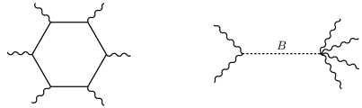
Figure 1: Ten-dimensional anomalies are determined by a one-loop hexagon diagram as the one shown on the left panel of this figure. In the GS mechanism, their contribution to the anomaly is canceled by tree-level diagrams as the one depicted on the right panel, describing the interchange of a $B$-field between gravitons and/or gauge bosons. Here and in all other diagrams below, the wavy lines represent either gauge or graviton fields, as explained in the text.

These modifications to the low-energy action provide the clue to understanding how the $B$-field cancels the anomaly at a diagrammatic level. We know that gauge and gravitational anomalies in a ten-dimensional field theory come from hexagon diagrams with gravitons and/or gauge bosons at the vertices (see the left panel of fig. 1). As explained in pag. 3, there are contributions from all diagrams containing an even number of gravitons and gauge bosons. Now, the presence of the Chern-Simons forms $\omega^{0}_{3}$ and $\Omega^{0}_{3}$ in the field strength (62) induces new interactions from the kinetic term (61): vertices with a single $B$-field and either two gravitons or two gauge bosons. Furthermore, the part of the GS counterterm shown in (63) introduces three additional five-point vertices. They contain one $B$-field and either four gravitons, four gauge bosons or two gravitons and two gauge bosons.

Due to these new interactions there are additional diagrams contributing to the anomaly. In particular the one shown on the right of fig. 1, where either two gravitons or two gauge bosons combine into a $B$-field that decays into either four gravitons, four gauge bosons or two gravitons and two gauge bosons. The GS mechanism works because these tree-level diagrams cancel the parity-violating contribution from the hexagons, rendering the theory anomaly-free. Notice that the source of parity violation in the tree diagram is entirely in the right vertex. The coupling of two gravitons or two gauge bosons and a $B$-field preserves parity due to presence of the Hodge dual in the kinetic term (61).

This diagrammatic interpretation brings forward the unusual character of the GS mechanism. Anomaly cancellation in quantum field theory usually proceeds by including either additional species or new couplings (or both), so the offending one-loop diagrams are canceled by other one-loop diagrams with either these extra states running in the loop or (and) new couplings showing up in the vertices. Not so in the GS mechanism. Here we have tree-level diagrams cancelling loops.

To understand why this happens, we go back to a comment on page 2 where we pointed out that anomalies can be seen as arising from IR poles in the expectation value of current, as opposed to UV ambiguities in the expectation values of the current divergence. The diagrams we are discussing contribute to the expectation value of the gauge current and the energy-momentum tensor, so anomalies are read from the residue of the parity-violating part of the hexagon diagram in the limit in which the invariant mass of the $i$-th and $j$-th insertions approaches zero, $s_{ij}=-2p_{i}\cdot p_{j}\rightarrow 0$. On the other hand, since the $B$-field is massless, its interchange in tree diagram on the right of fig. 1 generates a pole at zero-momentum transfer.

For the tree-level diagram to cancel the right poles from the hexagon a number of things have to conspire. The $B$-field is neutral and cannot transfer gauge charge from one vertex to the other. This means that no cancellation can take place on any pole proportional to a single trace over gauge generators, a situation that we avoided by restricting the gauge group to those for which these traces factorize. Similarly, lacking Lorentz indices, it cannot cancel poles proportional to ${\rm Tr\,}\mathcal{R}^{3}$ either. These are the terms that we got rid of in the hexagon by setting $N=496$.

Type-I superstrings and beyond.

The modifications to the field theory action of ten-dimensional $\mathcal{N}=1$ gauged SUGRA imposed by anomaly cancellation do not pose any problems within a field-theoretic context. Indeed, in quantum field theory we are always allowed the freedom of “building” a Lagrangian so it fits our low energy requirements. Any couplings we might need to introduce are swept under the rug of an eventual UV completion of the theory. There is however a problem when the theory we deal with describes the low-energy dynamics of some string model. Since string theory is UV complete, both the massless states and their couplings are fully determined. Our playground is thus pretty much constrained.

This is why we need to go a step further and check whether the GS mechanism is in fact fully implemented in type-I string theory. In other words, it is not enough having the appropriate antisymmetric tensor field in the spectrum, but the new coupling stemming from the modified field strength (62) and the GS counterterm proportional to $BX_{8}$ should actually follow from the low-energy limit of the string interactions up to the last factor.

Let us focus on pure gauge anomalies. There are three kinds of one-loop string diagrams contributing to them: the planar orientable annulus with all Yang-Mills vertex operators attached to a single boundary, the nonorientable Möbius strip with six gauge insertions on its boundary, and the nonplanar annulus with four vertices attached to one boundary and two to the other (remember that gauge bosons belong to the open string sector and therefore couple to the diagram boundaries). An explicit calculation GS2 shows that for SO(32) gauge anomalies cancel among the first two topologies, whose group theory factors are in both cases single traces ${\rm tr}_{\rm adj}(\lambda^{a_{1}}\ldots\lambda^{a_{6}})$. As to the nonplanar diagram shown on the left of fig. 2, it is proportional to ${\rm tr}_{\rm adj}(\lambda^{a_{1}}\lambda^{a_{2}}){\rm tr}_{\rm adj}(\lambda^{a_{3}}\ldots\lambda^{a_{6}})$ and does not contribute to the anomaly.

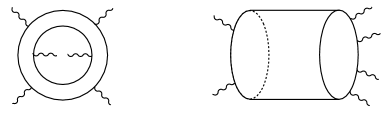
Figure 2: In type-I string theory the contribution of the nonplanar six-point annulus diagram on the left is recast in the closed-string channel as the tree-level diagram on the right. Closed string states, among them the R-R massless $B$-field, propagates along the cylinder resulting in the low-energy limit in the diagram shown on the right of fig. 1.

This proves that gauge anomalies cancel in full-fledged type-I string theory. To connect with the field-theoretic analysis of the GS mechanism, we need to look for the IR poles associated with the three diagrammatic topologies mentioned above. The two first topologies (the planar annulus and the Möbius strip) produce the poles associated to the field theory hexagon. Surprisingly, the nonplanar annulus on the left of fig. 2 also gives a massless pole. Switching from the open to the closed string channel, this diagram is transformed into one in which the gauge bosons interact with each other through the interchange of a closed string, as shown on the right of fig. 2. Close to the zero-momentum transfer, the amplitude is dominated by the boundary of the moduli space corresponding to a very long cylinder. Moreover, its parity-violating part is nonzero if the state running along the cylinder is the R-R rank-two antisymmetric tensor. For SO(32), the single trace in the planar annulus and Möbius strip topologies factorizes and its pole is canceled by the cylinder diagram, as required for the GS mechanism to work.

This proves that the GS mechanism is automatically implemented in type-I string theory, at least for gauge anomalies. The analysis of gravitational and mixed anomalies requires more work. Besides the topologies already considered, now with graviton vertex operators inserted in their interior, we need to compute the contributions of the torus and the Klein bottle, both with and without a boundary. Their explicit evaluation open_gen_anom_anal shows that all anomalies cancel at one loop. The interpretation of the tree-level diagram is now a little bit different. The relevant parity-violating pole comes again from the $B$-field propagating along a long cylinder. However, depending on the amplitude there are three separate possibilities: the cylinder has two gauge boson insertions on one of its boundaries while the other one is attached to a torus with four graviton vertex operators; it joints a sphere with two gravitons to a torus with four gravitons (cf. the diagram on the right of fig. 3 below); or it connects a sphere with two gravitons to a torus with a boundary and two gauge bosons attached to it, while two graviton vertex operators are also inserted in its bulk.

It is difficult to exaggerate the importance of the discovery of the GS mechanism in the historical development of string theory. After the doubts sown by the results of AG_Witten concerning the consistency of type-I string theory, the discovery of a highly nontrivial cancellation mechanism meant a very important push to the theory, so important that with it the first superstring revolution was initiated. One of the consequences was the attempts to accommodate the second “safe” group $E_{8}\times E_{8}$ into the framework of string theory. This led to the formulation of the heterotic string princeton_quartet , the model that dominated string phenomenology until the advent of D-branes at the onset of the second superstring revolution.

The low-energy dynamics of the heterotic string is also that of $\mathcal{N}=1$ SUGRA coupled to $\mathcal{N}=1$ SYM, although in a slightly modified fashion from the one we encountered for type-I strings chapline_manton . This notwithstanding, the theory contains the crucial rank-two antisymmetric tensor field, this time in the NS-NS sector, and the implementation of the GS mechanism follows the same steps outlined above. The absence of an open string sector means that in the heterotic string the calculation of the anomaly only involves a single diagram, a torus with six graviton/gauge boson vertex operators as the one shown on the left of 3. The key to the cancellation of spacetime anomalies in the heterotic string lies in modular invariance heterotic_anomalies , the very same symmetry restricting the allowed gauge groups to SO(32) and $E_{8}\times E_{8}$.

Anomalies in the heterotic string are associated with contributions coming from the boundary of the moduli space of tori with six punctures. If the theory is modular invariant, this boundary has two components whose contributions cancel each other out: the limit $\tau\rightarrow i\infty$, corresponding to very long tori, and the limit in which the $i$-th and $j$-th punctures collide. In the first case, the diagram is dominated by massless states running along the torus and its parity-violating piece gives the pole associated with the field theory hexagon diagram. The second component corresponds to the factorization limit where the punctured torus degenerates into a sphere containing the two colliding vertex operators joined by a long cylinder to a torus with the remaining insertions (see the drawing on the right of fig. 3). The associated parity-violating pole comes from the propagation of the $B$-field along the cylinder, thus implementing the GS cancellation mechanism in the low-energy field theory.

         

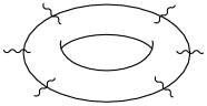
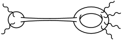
Figure 3: All gauge and gravitational anomalies in the heterotic string stem from the torus diagram shown on the left. Low-energy poles from the field theory hexagon are canceled by the ones coming from massless closed string states running in the long propagator joining the sphere and the torus in the diagram on the right. This diagram also occurs in the calculation of the pure gravitational anomaly of type-I string theory.

Some further examples of the GS mechanism

The GS mechanism, first identified in the context of type-I string theory, has found implementation in various secenarios. Here we discuss three particular instances of this anomaly cancellation mechanism at work.

The ${\bf\mathrm{\bf SO}(16)\bm{\times}\mathrm{\bf SO}(16)}$ nonsupersymmetric string. The $\mathrm{SO}(16)\times\mathrm{SO}(16)$ heterotic string SO(16) is a ten-dimensional nonsupersymmetric and tachyon-free fermionic model. Its spectrum, besides the universal gravity multiplet containing the graviton, dilaton, and antisymmetric rank-two tensor field, includes a positive and a negative chirality Majorana-Weyl fermions respectively transforming in the $(\bm{16},\bm{16})$ and $(\bm{128},\bm{1})\oplus(\bm{1},\bm{128})$ representations of $\mathrm{SO}(16)\times\mathrm{SO}(16)$, with $\bm{16}$ and $\bm{128}$ the fundamental and spinor representations of SO(16). Since these are the only fields contributing to the anomaly, we can write the relevant anomaly polynomial as

$$I_{12}={1\over 2}I_{1\over 2}[\mathcal{F},\mathcal{R}]_{(\bm{16},\bm{16})}-{1\over 2}I_{1\over 2}[\mathcal{F},\mathcal{R}]_{(\bm{128},\bm{1})}-{1\over 2}I_{1\over 2}[\mathcal{F},\mathcal{R}]_{(\bm{1},\bm{128})},$$ (64)

where once more the ${1\over 2}$ factors account for the number of degrees of freedom of a Majorana-Weyl spinor and the subscripts remind us what representation we should use to evaluate the traces in the corresponding Chern characters. It is a peculiarity of this model that, unlike the type-I superstring, we have fermions transforming in various representations of the gauge group. Interestingly, looking at eq. (44) we see that all pure gravitational anomaly terms cancel among each other, due to the identity $16^{2}-128-128=0$.

We are left then with pure and mixed gauge anomalies. In order to check their cancellation it is convenient to write all Chern characters using traces in the fundamental representation $\bm{16}$ of SO(16). Remarkably, when this is done SO(16) we find the factorized result

$$I_{12} =(\mbox{ch}_{2}+\mbox{ch}_{2}^{\prime}-p_{1})X_{8},$$ (65)

where the prime indicates the second factor of SO(16) and $X_{8}$ is explicitly given by

$$X_{8}={1\over 2}\big{(}\mbox{ch}_{4}+\mbox{ch}^{\prime}_{4}\big{)}-{1\over 48}\big{(}\mbox{ch}_{2}^{2}+\mbox{ch}_{2}^{\prime 2}-\mbox{ch}_{2}\mbox{ch}^{\prime}_{2}\big{)}.$$ (66)

Since the $\mbox{SO(16)}\times\mbox{SO(16)}$ heterotic string contains a rank-two antisymmetric tensor in its gravity multiplet, we can repeat the analysis presented above for the type-I string and conclude that all anomalies cancel through the GS mechanism. $\blacksquare$

Type-I string theory with space-filling D- and anti-D-branes. We consider next the GS cancellation mechanism for type-IIB strings in the presence of one orientifold O9-plane and a stack of $m$ D9-branes and $n$ anti-D9-branes sugimoto . The gauge group is $\mbox{SO}(m)\times\mbox{SO}(n)$ and the charged massless chiral fields are a positive chirality fermion in the adjoint of SO($m$), a positive chirality fermion in the symmetric tensor representation of SO($n$), and a negative chirality spinor in the bifundamental of $\mbox{SO}(m)\times\mbox{SO}(n)$. These are excitations of open strings with endpoints attached to two D9-branes, two anti-D9-branes, and one D9-brane and one anti-D9-brane respectively. Adding to this the contributions of the positive helicity gravitino and the negative helicity dilatino, the 12-form anomaly polynomial is given by

$$I_{12} =-{1\over 2}I_{1\over 2}[\mathcal{R}]+{1\over 2}I_{3\over 2}[\mathcal{R}]+{1\over 2}I_{1\over 2}[\mathcal{F},\mathcal{R}]_{({\rm adj},\bm{1})}$$

$$+{1\over 2}I_{1\over 2}[\mathcal{F},\mathcal{R}]_{(\bm{1},{\rm sym})}-{1\over 2}I_{1\over 2}[\mathcal{F},\mathcal{R}]_{({\rm f},{\rm f})},$$ (67)

where the explicit expression for each term can be found in eqs. (37), (38), and (44). We just look at the two terms spelling trouble for the implementation of the GS mechanism, which are the ones containing $p_{3}$ and $\mbox{ch}_{6}$. The first one is proportional to

$$496-{1\over 2}m(m-1)-{1\over 2}n(n+1)-mn=496-{1\over 2}(m-n)(m-n-1),$$ (68)

which cancels for $m-n=32$. As to the second offending term, we search for identities relating the traces of $\mathcal{F}^{6}$ in the various representations to those in the fundamental. The relevant ones are

$${\rm tr}_{({\rm adj},\mathbf{1})}\mathcal{F}^{6} =(n-32){\rm tr}_{\rm f}\mathcal{F}^{6}+15\big{(}{\rm tr}_{\rm f}\mathcal{F}^{2}\big{)}\big{(}{\rm tr}_{\rm f}\mathcal{F}^{4}\big{)},$$

$${\rm tr}_{(\mathbf{1},{\rm sym})}\mathcal{F}^{6} =(m+32){\rm tr}_{\rm f}\mathcal{F}^{\prime 6}+15\big{(}{\rm tr}_{\rm f}\mathcal{F}^{\prime 2}\big{)}\big{(}{\rm tr}_{\rm f}\mathcal{F}^{\prime 4}\big{)},$$ (69)

$${\rm tr}_{({\rm f},{\rm f})}\mathcal{F}^{6} =n{\rm tr}_{\rm f}\mathcal{F}^{6}+m{\rm tr}_{\rm f}\mathcal{F}^{\prime 6},$$

where the primes indicate the field strength associated to the SO($n$) factor. Adding these three contributions with their respective signs, we find a cancellation of the irreducible terms proportional to ${\rm tr\,}\mathcal{F}_{1}^{6}$ and ${\rm tr\,}\mathcal{F}_{2}^{6}$. This ensures the factorization of the anomaly polynomial

$$I_{12}=\left(p_{1}-{1\over 30}\mbox{ch}_{2}-{1\over 30}\mbox{ch}^{\prime}_{2}\right)Y_{8}$$ (70)

where

$$Y_{8} =-{1\over 48}\left[{\rm ch}_{4}-{\rm ch}^{\prime}_{4}-{1\over 60}p_{1}\big{(}{\rm ch}_{2}-{\rm ch}^{\prime}_{2}\big{)}+{3\over 8}p_{1}^{2}-{1\over 2}p_{2}\right],$$ (71)

and the prime again indicates the Chern characters associated with SO($n$). All gauge, gravitational, and mixed anomalies thus cancel for $m-n=32$ through the GS mechanism. As in the case of the type-I string, we also need to modify the antisymmetric tensor field strength

$$H=dC_{2}-{1\over 30}\omega_{3}^{0}-{1\over 30}\omega^{\prime 0}_{3}+\Omega_{3}^{0},$$ (72)

and add the corresponding GS counterterm to the action

$$\Gamma_{\rm ct}=c\int_{\mathcal{M}_{10}}C_{2}Y_{8}+{1+\alpha\over 2}c\int_{\mathcal{M}_{10}}\left({1\over 30}\omega_{3}^{0}+{1\over 30}\omega^{\prime 0}_{3}-\Omega^{0}_{3}\right)Y_{7}^{0},$$ (73)

with $Y_{8}=dY_{7}^{0}$.$\blacksquare$

A four-dimensional version of the GS mechanism. As a final example, we study the implementation of the GS mechanism in a purely field-theoretical setup. Let us consider the theory of a positive chirality Weyl fermion coupled to a U(1) gauge field propagating, for simplicity, on flat spacetime. The corresponding anomaly polynomial is

$$I_{6}=\mbox{ch}_{3},$$ (74)

and the theory has an anomaly given by

$$\delta_{\eta}S_{\rm eff} =2\pi i\int\omega^{1}_{4}=-\int\eta\mbox{ch}_{2},$$ (75)

where we have used that $\omega^{1}_{4}$ is proportional to $\mathcal{F}^{2}$ and therefore to the second Chern character.

For a U(1) gauge group, the anomaly polynomial (74) trivially factors

$$\mbox{ch}_{3}={1\over 3}\mbox{ch}_{1}\mbox{ch}_{2},$$ (76)

and the GS mechanism is implemented by an axion field $\theta$ with the gauge transformation

$$\delta_{\eta}\theta=m_{\rm GS}\eta.$$ (77)

and a gauge-invariant kinetic term

$$S\supset{1\over 2}\int\big{(}d\theta-m_{\rm GS}\mathcal{A}\big{)}\wedge\star\big{(}d\theta-m_{\rm GS}\mathcal{A}\big{)}.$$ (78)

Here, $m_{\rm GS}$ is a constant with dimensions of mass. The anomaly is then canceled by the addition of the four-dimensional GS counterterm

$$S_{\rm ct}=-{1\over m_{\rm GS}}\int\theta\mbox{ch}_{2}={1\over 8\pi^{2}m_{\rm GS}}\int\theta\mathcal{F}^{2}.$$ (79)

Indeed, $\delta_{\eta}S_{\rm eff}+\delta_{\eta}S_{\rm ct}=0$ and gauge invariance is preserved quantum-mechanically.

This cancellation can also be understood in diagrammatic terms by noticing that (78) introduces a kinetic mixing between the axion and the gauge field of the form $\mathcal{A}^{\mu}\partial_{\mu}\theta$. On the other hand, the counterterm (79) induces a trivalent vertex with one axion and two gauge fields. Thus, the triangle diagram producing the anomaly (75) is canceled by a tree-level diagram where a gauge field transmutes into an axion that then decays into two other gauge fields. This is the four-dimensional analog of the diagram shown on the right panel of fig. 1. In fact, the axion is just a two-form field in disguise, since both fields are related by Hodge duality in four dimensions, $d\theta=\star dB$ bonnefoy_dudas . $\blacksquare$

5 Anomaly inflow

Having focused so far on anomaly cancellation, our discussion has avoided the evaluation of currents. In the gauge case, the (consistent) current is obtained by taking variations of the nonlocal quantum effective action $\Gamma_{\rm eff}$ with respect to the gauge one-form $\mathcal{A}$. The result splits into two pieces, one given by an integral over the “bulk” $\mathcal{M}_{2n-1}$ space and a second defined on its $(2n-2)$-dimensional boundary

$$\delta\Gamma_{\rm eff}=\int_{\mathcal{M}_{2n-1}}{\rm Tr\,}\big{(}J_{\rm bulk}\delta\mathcal{A}\big{)}+\int_{\partial\mathcal{M}_{2n-1}}{\rm Tr\,}\big{(}X\delta\mathcal{A}\big{)}.$$ (80)

The quantities inside the traces in both integrals are explicitly given by

$$J_{\rm bulk} ={i^{n}\over(n-1)!(2\pi)^{n-1}}\mathcal{F}^{n-1},$$

$$X ={i^{n}\over(n-1)!(2\pi)^{n-1}}\int_{0}^{1}tdt\,\Big{(}\mathcal{F}_{t}^{n-2}\mathcal{A}+\mathcal{F}_{t}^{n-3}\mathcal{A}\mathcal{F}_{t}+\ldots+\mathcal{A}\mathcal{F}_{t}^{n-2}\Big{)},$$ (81)

with $\mathcal{F}_{t}\equiv t\mathcal{F}+t(t-1)\mathcal{A}^{2}$. We particularize (80) to the case of infinitesimal gauge transformations, $\delta_{\chi}\mathcal{A}=d\chi+[\mathcal{A},\chi]\equiv D\chi$, where $D$ denotes the gauge covariant derivative. Applying the Stokes theorem, we find the gauge variation of the effective action

$$\delta_{\chi}\Gamma_{\rm eff}=-\int_{\mathcal{M}_{2n-1}}{\rm Tr\,}\big{(}\chi DJ_{\rm bulk}\big{)}+\int_{\partial\mathcal{M}_{2n-1}}{\rm Tr\,}\Big{[}\chi\big{(}J_{\rm bulk}-DX\big{)}\Big{]}.$$ (82)

As we know, the left-hand side of this equation gives the consistent anomaly [cf. (1)], which we express in terms of the consistent current $J_{\rm cons}$ as

$$\delta_{\chi}\Gamma_{\rm eff}\equiv-\int_{\partial\mathcal{M}_{2n-1}}{\rm Tr\,}\big{(}\chi DJ_{\rm cons}\big{)}.$$ (83)

As to the right-hand side of (82), the first thing to notice is that the Bianchi identity $D\mathcal{F}=0$ implies $DJ_{\rm bulk}=0$ so the first, nonlocal term vanishes. In addition to this, the quantity $X$ defined in (81) is minus the Bardeen-Zumino term BZ_NPB relating the consistent and covariant currents, $J_{\rm cov}=J_{\rm cons}-X$ (see our discussion in page 2). We thus obtain a very suggestive expression

$$DJ_{\rm cov}=-J_{\rm bulk}\bigg{|}_{\partial\mathcal{M}_{2n-1}},$$ (84)

stating that the covariant anomaly equals minus the bulk current evaluated at the boundary.

To understand the implications of this relation, let us take a step back and review what we have done. By expressing it as an integral over a higher-dimensional space, the nonlocal effective action $\Gamma_{\rm eff}$ can be interpreted as describing the local quantum effective dynamics of gauge fields interacting with Dirac fermions in the odd-dimensional bulk Euclidean spacetime $\mathcal{M}_{2n-1}$. This theory is free of gauge anomalies, as it is manifest in the fact that the quantum current $J_{\rm bulk}$ is conserved, $DJ_{\rm bulk}=0$. The situation is quite different on the even-dimensional boundary theory, which contains chiral fermions and where $DJ_{\rm cov}$ (or $DJ_{\rm cons}$ for that matter) has a nonvanishing value, signaling the existence of a gauge anomaly. Equation (84) provides the clue to understand physically what is going on: the gauge anomaly results from the inflow of gauge charge from the bulk onto the boundary, as shown by the fact that the value of the bulk current there precisely cancels the rate of nonconservation of the gauge charge.

This general argument illustrates the basic features of the mechanism of anomaly inflow first pointed out in CH (see also harvey_review for a review). Anomalous theories can be embedded in higher-dimensional, anomaly-free theories so that violations in the conservation of charge are accounted for by the inflow of charge from the higher-dimensional bulk. Or the other way around, nonanomalous theories in the presence of topological defects may have anomalies supported on their worldvolumes, which are nevertheless canceled by the charge flowing from outside the defect.

A simple example of anomaly inflow

Let us see the workings of anomaly inflow in a particular example, that of a massless Dirac fermion in 3+1 dimensions in the presence of an axion string defect CH ; BH ; harvey_review . The relevant terms in the action are

$$S=\int d^{4}x\,\Big{[}i\overline{\psi}\gamma^{\mu}\partial_{\mu}\psi+\overline{\psi}\big{(}\varphi_{1}+i\gamma_{5}\varphi_{2}\big{)}\psi\Big{]}.$$ (85)

Here, $\varphi\equiv\varphi_{1}+i\varphi_{2}$ is a complex scalar field in the vacuum configuration

$$\varphi(x) =f(\rho)e^{i\theta(x)},$$ (86)

where $\rho^{2}=(x^{1})^{2}+(x^{2})^{2}$ and $f(\rho)$ satisfies $f(\rho\rightarrow 0)=0$ and $f(\rho\rightarrow\infty)=v$. This describes a stringlike vortex localized along the $x^{3}\equiv z$ direction.

The massless Dirac fermion contains two opposite chiralities and can be coupled to an electromagnetic U(1) without gauge anomalies. The question however is whether the string defect supports chiral fermion modes that might induce anomalies on its worldvolume. To clarify the issue, we split the Dirac fermion into its two chiralities $\gamma_{5}\psi_{\pm}=\pm\psi_{\pm}$ and separate the string worldvolume directions $x^{a}\equiv(x^{0},x^{3})$ from the transverse coordinates $(x^{1},x^{2})=(\rho\cos\phi,\rho\sin\phi)$. We also factorize the four-dimensional chirality matrix $\gamma_{5}=i\gamma^{0}\gamma^{1}\gamma^{2}\gamma^{3}$ as $\gamma_{5}=\overline{\gamma}\gamma_{T}$, where $\overline{\gamma}=-\gamma^{0}\gamma^{3}$ is the two-dimensional chirality matrix and $\gamma_{T}\equiv-i\gamma^{1}\gamma^{2}$. Doing all this, the Dirac equation is recast as the pair of equations

$$i\gamma^{a}\partial_{a}\psi_{\pm}+i\gamma^{2}\big{(}\cos\phi+i\overline{\gamma}_{T}\sin\phi\big{)}\partial_{\rho}\psi_{\pm}=f(\rho)e^{\mp i\phi}\psi_{\mp}.$$ (87)

admitting the solution

$$\psi_{-} =\eta(x^{a})\exp\left[-\int_{0}^{\rho}d\rho^{\prime}f(\rho^{\prime})\right],$$

$$\psi_{+} =-i\gamma^{2}\psi_{-}.$$ (88)

Here $\eta$ is a negative chirality spinor satisfying the two-dimensional Dirac equation on the string worldvolume

$$i\gamma^{a}\partial_{a}\eta=0,\hskip 28.45274pt\overline{\gamma}\eta=-\eta.$$ (89)

We have shown the existence of a zero mode in the bulk Dirac equation corresponding to a massless spinor along the string defect whose chirality is correlated with its direction of propagation, $(\partial_{0}-\partial_{3})\eta=0$. As a consequence, when coupling the theory to an external electromagnetic field $\mathcal{A}_{\mu}$, the chiral zero mode triggers a gauge anomaly on the string worldvolume

$$\partial_{a}J^{a}={e\over 4\pi}\epsilon^{ab}\mathcal{F}_{ab}={e\mathcal{E}\over 2\pi},$$ (90)

with $\mathcal{E}$ the external electric field along $x^{3}$. This expression gives the amount of charge nonconservation per unit time and unit length. Notice that (90) gives the covariant anomaly, which in two dimensions is one-half the value of the consistent anomaly (for an explicit calculation of the consistent anomaly in this case, see, for example, QFT_book ). Let us recall that this happens on a string defect otherwise embedded in a theory that as a whole is free from gauge anomalies.

To give a physical picture of what is going on, we study the bulk theory outside the string defect and compute the one-loop corrected gauge current in the presence of the soliton $\varphi$. In the adiabatic approximation where scalar field gradients are small, this is given by the Goldstone-Wilczek current GW

$$\langle J^{\mu}\rangle_{\rm bulk}=-{ie\over 16\pi^{2}}\epsilon^{\mu\nu\alpha\beta}{\varphi^{*}\partial_{\nu}\varphi-\varphi\partial_{\nu}\varphi^{*}\over|\varphi|^{2}}\mathcal{F}_{\alpha\beta}.$$ (91)

Evaluating it on the vacuum solution (86) and in the region where $f(\rho)$ is well approximated by its asymptotic value, we get

$$\langle J^{\mu}\rangle_{\rm bulk}={e\over 8\pi^{2}}\epsilon^{\mu\nu\alpha\beta}\partial_{\nu}\theta\mathcal{F}_{\alpha\beta}.$$ (92)

To clarify the workings of anomaly inflow in this case, let us take a gauge configuration describing an electric field $\mathcal{E}$ along $x^{3}=z$. Thus, $\mathcal{F}_{ab}=\mathcal{E}\epsilon_{ab}$ with all remaining components of the field strength equal to zero. The bulk electric current can then be written as

$$\langle\bm{J}\rangle_{\rm bulk}=-{e\mathcal{E}\over 4\pi^{2}}(\boldsymbol{\bm{\nabla}}\theta)\times\mathbf{u}_{z}.$$ (93)

Moreover, for an axion string solution we have $\theta(x)=\phi$, so the previous result takes the simpler form

$$\langle\bm{J}\rangle_{\rm bulk}=-{e\mathcal{E}\over 4\pi^{2}\rho}\mathbf{u}_{\rho}.$$ (94)

This shows the existence of radial charge transport from the bulk towards the defect. Computing the flux of the bulk current (94) through a cylindrical surface centered on the string, we find the incoming charge per unit length and unit time to be

$${dQ\over dtdL}={e\mathcal{E}\over 2\pi},$$ (95)

which exactly reproduces the rate of violation of electric charge conservation on the string worldvolume, as given in eq. (92). The gauge anomaly on the defect is thus canceled by the inflow of charge from the bulk.

Our presentation here has closely followed ref. CH . It is possible nevertheless to recast the analysis in a language similar to the one used at the beginning of this section. We start with the bulk effective action describing an axion field coupled to the electromagnetic field

$$S_{\rm axion}=-{e^{2}\over 8\pi^{2}}\int_{V}\theta\mathcal{F}^{2},$$ (96)

and take variations with respect to the gauge field

$$\delta S_{\rm axion}={e^{2}\over 4\pi^{2}}\int_{V}d\theta\mathcal{F}\delta\mathcal{A}-{e^{2}\over 4\pi^{2}}\int_{\partial V}\theta\mathcal{F}\delta\mathcal{A}.$$ (97)

Here we assumed that all fields go to zero at infinity and take $\partial V$ a cylindrical surface surrounding the axion string. The expression obtained exhibits the structure displayed in eq. (80), so we identify

$$J_{\rm bulk} ={e\over 4\pi^{2}}d\theta\mathcal{F},$$ (98)

where we absorbed a power of $e$ into $\delta\mathcal{A}$. This is equivalent to eq. (92) and using (84) we retrieve the two-dimensional covariant anomaly (90) naculich . $\blacksquare$

Anomalous D-brane couplings.

Due to its universal nature, anomaly inflow is at work in a wide range of physical situations, ranging from condensed matter and fluid dynamics to lattice field theory and string theory. As to the last field, Polchinski’s discovery of D-branes dbranes_polchinski as the sources of R-R charge not only solved a long-standing riddle. It also put the focus on the plethora of extended solitonic defects present in string theory, many of which had been already studied in the realm of supergravity (see DKL for a contemporary review on the issue). It is only natural that anomaly inflow found immediate application in this context.

In a consistent string theory, any anomaly supported on the worldvolume of a defect (D-branes, orientifolds, NS-branes,…) has to be canceled by charge inflow from the bulk. The condition for this to happen determines the gauge and gravitational couplings of the extended object GHM ; CY (see also johnson ; szabo for reviews). Let us see how this works in a case that looks very much like a generalization of the axion string discussed in page 5. We consider a $(p+1)$-form field $C_{p+1}$ coupled to a $p$-brane embedded in a $D$-dimensional flat space $\mathcal{M}_{D}$. The relevant terms in the bulk low-energy action are

$$S\supset-{1\over 4}\int_{\mathcal{M}_{D}}H_{p+2}\wedge\star H_{p+2}+{\mu_{p}\over 2}\int_{\mathcal{B}_{p}}C_{p+1},$$ (99)

where $H_{p+2}=dC_{p+1}$ is the gauge-invariant field strength and $\mathcal{B}_{p}$ the $(p+1)$-dimensional brane worldvolume. The associated equations of motion show that $C_{p+1}$ is sourced by the $p$-brane

$$d\star H_{p+2}=\mu_{p}\delta_{D-p-1}(\mathcal{B}_{p+1}\hookrightarrow\mathcal{M}_{D}),$$ (100)

where we introduced a $(D-p-1)$-form delta function satisfying

$$\int_{\mathcal{M}_{D}}\delta_{D-p-1}(\mathcal{B}_{p}\hookrightarrow\mathcal{M}_{D})\alpha_{p+1}=\int_{\mathcal{B}_{p}}\alpha_{p+1},$$ (101)

for any $(p+1)$-form $\alpha_{p+1}$ defined on $\mathcal{B}_{p+1}$. A look at eq. (100) indicates that the Hodge dual of this object can be interpreted as a worldvolume-supported $(p+1)$-form current $J_{p+1}$

$$\star J_{p+1}=\delta_{D-p-1}(\mathcal{B}_{p}\hookrightarrow\mathcal{M}_{D}),$$ (102)

so the equations of motion for $C_{p+1}$ are recast as $d\star H_{p+2}=\mu_{p}\star J_{p+1}$.

Let us take $p$ to be odd and assume that the $p$-brane worldvolume supports a chiral fermion zero mode leading to gauge anomalies. From eq. (10) we know that the anomalous variation of the brane action is given by

$$\delta S_{\rm brane}=2\pi i\int_{\mathcal{B}_{p}}I_{p+1}^{1},$$ (103)

where $dI_{p+1}^{1}=\delta I_{p+2}^{0}$, with $I_{p+2}^{0}$ the Chern-Simons descended from the brane anomaly polynomial $I_{p+3}$. If the bulk theory on $\mathcal{M}_{D}$ is anomaly-free, its action should contain the coupling

$$\Delta S_{\rm bulk}={2\pi i\over\mu_{p}}\int_{\mathcal{M}_{D}}\star H_{p+2}\wedge I^{0}_{p+2},$$ (104)

whose gauge variation cancels the anomaly on the brane (103)

$$\delta\Delta S_{\rm bulk}=-{2\pi i\over\mu_{p}}\int_{\mathcal{M}_{D}}d\star H_{p+2}\wedge I_{p+1}^{1}=-2\pi i\int_{\mathcal{B}_{p+1}}I_{p}^{1}.$$ (105)

In the second identity we have used the equations of motion (100). Just by requiring that anomaly inflow restores the consistency of theory we determined the coupling in eq. (104). The other way around, a computation of the term (104) from the bulk theory determines $\mu_{p}$, measuring the coupling of the $p$-brane to $C_{p+1}$.

We want to apply the philosophy of this calculation to the case of D$p$-branes. We might be tempted to consider the vanilla case of a single flat D$p$-brane in flat space (or a parallel stack of them). In type-IIB theory $p$ takes odd values so the $(p+1)$-dimensional D-brane worldvolume is even-dimensional and may contain chiral fermions. Yet, there is the same number of positive and negative chirality fermions on the brane, all in the adjoint representation of the gauge group. This means that the theory is anomaly-free. Another way to understand the absence of gauge brane anomalies in this setup is by taking into account that the bulk type-IIB theory does not contain gauge fields. Were the theory on the brane anomalous, its anomaly would have no chance of being canceled by accretion/depletion of gauge charge from the ten-dimensional bulk.

We need to consider less simple configurations including also the effects of gravitational anomalies. One interesting scenario is that of intersecting branes whose combined worldvolumes span the whole ten-dimensional spacetime while producing a chiral theory at an even-dimensional intersection GHM . Anomalies there are compensated by the inflow of charge from the “parent” D-branes worldvolumes. The condition for this cancellation to happen determines the anomalous gauge and gravitational couplings of the D$p$-brane.

Another way to generate a chiral theory on a D$p$-brane, with $p$ odd, is by playing with curvature CY . Let us consider a stack of $N$ coincident D$p$-branes whose worldvolume wrap $\mathcal{B}_{p+1}$. In this D-brane background the ten-dimensional local Lorentz group $\mbox{SO}(1,9)$ breaks down to $\mbox{SO}(1,p)\times\mbox{SO}(9-p)$, where the first factor is the local Lorentz group on the brane worldvolume and the second the $R$-symmetry of the maximal SYM theory describing the dynamics on the brane. This breaking of the structure group of the tangent bundle $T\!\mathcal{M}$ reflects its decomposition into a Whitney sum of the brane tangent and normal bundles

$$T\!\mathcal{M}=T\!\mathcal{B}_{p}\oplus TN.$$ (106)

At the same time, fermions in the $\bm{16}$ Majorana-Weyl representation of $\mbox{Spin}(1,9)$ split into representations of $\mbox{Spin}(1,p)\times\mbox{Spin}(9-p)$ with correlated chiralities. As an example, for $p=3$ we have the $(\bm{2},\bm{4})\oplus(\overline{\bm{2}},\overline{\bm{4}})$ representation of $\mbox{Spin}(1,3)\times\mbox{Spin}(6)$, whereas for $p=5$ the $\bm{16}$ of $\mbox{Spin}(1,9)$ decomposes as $(\bm{4}_{\bm{p}},\bm{2}_{\bm{p}})\oplus(\bm{4}^{\prime}_{\bm{p}},\bm{2}^{\prime}_{\bm{p}})$. Incidentally, the previous examples display an interesting general property: for $p=1$ mod 4 the two spinor chiralities transform in independent representations of $\mbox{Spin}(9-p)$, whereas when $p=3$ mod 4 they are complex conjugate of each other (see, for example, seiberg_rev ).

The group $\mbox{Spin}(9-p)$ is a gauge invariance of the theory whose gauge potential is given by the normal space components of the spin connection, $\omega_{N}$. In addition, chiral fermions on the brane also have U($N$) Chan-Paton quantum numbers. Being massless excitations of open string with endpoints lying on a brane of the stack, they transform in its $\mbox{\bf N}\otimes\overline{\mbox{\bf N}}$ representation, which is real and therefore “safe” from the point of view of anomalies (in other words, U($N$) transformations are chirality-blind). In the mathematical lingo what we have is a vector bundle $(V\otimes S_{N}^{+})\oplus(V\otimes S_{N}^{-})$, where $V$ is the Chan-Paton bundle and $S^{\pm}_{N}$ are the spin bundles over the normal space associated with each chirality.

The only source of anomalies on the brane worldvolume are chiral fermions, so the anomaly polynomial is given by [cf. (11)]

$$I ={1\over 2}\widehat{A}(\mathcal{B}_{p})\big{[}\mbox{ch}(V\otimes S^{+}_{N})-\mbox{ch}(V\otimes S^{-}_{N})\big{]}$$

$$={1\over 2}\widehat{A}(\mathcal{B}_{p})\mbox{ch}(V)\big{[}\mbox{ch}(S^{+}_{N})-\mbox{ch}(S^{-}_{N})\big{]},$$ (107)

where the factor of ${1\over 2}$ in front accounts for Majorana-Weyl fermions and we have implemented the factorization property of the Chern character for product vector bundles, $\mbox{ch}(U\otimes W)=\mbox{ch}(U)\mbox{ch}(W)$. The Chern character of the Chan-Paton bundle can be further rewritten as

$$\mbox{ch}(V) \equiv\mbox{ch}_{\mathbf{N}\otimes\overline{\mathbf{N}}}(\mathcal{F})=\mbox{ch}_{\mathbf{N}}(\mathcal{F})\mbox{ch}_{\overline{\mathbf{N}}}(\mathcal{F})=\mbox{ch}(\mathcal{F})\mbox{ch}(-\mathcal{F}).$$ (108)

In the last equality we used the Hermitian character of the U($N$) generators and dropped the subscript with the understanding that all traces are computed in the fundamental representation of U($N$). With this, eq. (107) is recast as

$$I ={1\over 2}\widehat{A}(T\!\mathcal{B}_{p})\mbox{ch}(\mathcal{F})\mbox{ch}(-\mathcal{F})\big{[}\mbox{ch}(S^{+}_{N})-\mbox{ch}(S^{-}_{N})\big{]}.$$ (109)

Here it is manifest that the anomaly results from the asymmetry between $S^{+}_{N}$ and $S^{-}_{N}$. It remains to see how this is related to the curvature of the normal bundle, $\mathcal{R}_{N}=d\omega_{N}+\omega_{N}^{2}$.

To achieve this, we need an object that somehow we managed to do without so far, the Euler class. For a manifold $\mathcal{M}$ of dimension $2k$, the Euler class $e(\mathcal{M})$ is defined as the $2k$-form

$$e(\mathcal{M})=x_{1}\ldots x_{k},$$ (110)

where $x_{i}$ are again the skew eigenvalues introduced in eq. (17). The Euler class is thus the Pfaffian of ${1\over 2\pi}\mathcal{R}^{a}_{\,\,\,b}$ or, equivalently, the square root of the maximal Pontrjagin class. With this new polynomial at hand, we apply the general relation (see, for example, nash )

$$\mbox{ch}(S^{+}_{\mathcal{M}})-\mbox{ch}(S^{-}_{\mathcal{M}})=\prod_{i=1}^{k}\Big{(}e^{x_{i}/2}-e^{-x_{i}/2}\Big{)}={e(\mathcal{M})\over\widehat{A}(\mathcal{M})},$$ (111)

and rewrite the anomaly polynomial on the brane (109) as

$$I ={1\over 2}\mbox{ch}(\mathcal{F})\mbox{ch}(-\mathcal{F}){\widehat{A}(T\!\mathcal{B}_{p})\over\widehat{A}(TN)}e(TN).$$ (112)

Using the explicit expression of the $A$-roof in (22), the quotient in the previous equation can be expanded in terms of the Pontrjagin classes for the tangent and normal bundle, $p_{i}(\mathcal{R}_{T})\equiv p_{i}$ and $p_{i}(\mathcal{R}_{N})\equiv p_{i}^{\prime}$

$${\widehat{A}(T\!\mathcal{B}_{p})\over\widehat{A}(TN)} =1-{1\over 24}\big{(}p_{1}-p_{1}^{\prime})$$

$$+{1\over 5760}\big{(}7p_{1}^{2}+3p^{\prime 2}_{1}-10p_{1}p_{1}^{\prime}-4p_{2}+4p_{2}^{\prime}\big{)}+\ldots$$ (113)

Notice how the chiral asymmetry is controlled by the curvature of the normal bundle: setting $\mathcal{R}_{N}=0$ implies $e(TN)=0$ and the anomaly polynomial vanishes.

We have completed half our task. Brane anomalies are then computed from the polynomial (112) following the standard descend method: we extract its $p+3$-form piece $I_{p+3}=dI_{p+2}^{0}$ and get the anomaly as $\delta I^{0}_{p+2}=dI^{1}_{p+1}$. In a consistent theory this has to be canceled by charge inflow from the bulk.

This is the condition we are imposing now to determine the couplings of the D$p$-brane to the various R-R fields of type-IIB string theory. Let us define the field

$$C\equiv\sum_{k=0}^{5}C_{2k},$$ (114)

and assume that its dynamics is described by the action

$$S_{\rm RR}=-{1\over 4}\int_{\mathcal{M}_{10}}H\wedge\star H-{1\over 2}\sum_{k}\mu_{k}\int_{\mathcal{B}_{k}}CY_{k},$$ (115)

where $H\equiv dC$ is the field strength. In the previous ansatz we have introduced coupling constants $\mu_{k}$ to the different D-branes, while $Y_{k}$ are invariant polynomials built from the brane gauge field strength and the curvature. Their overall normalization is chosen so they can be written as $Y_{k}=N_{k}+dY_{k}^{0}$, with $N_{k}$ the number of D-branes wrapping on the worldvolume $\mathcal{B}_{k}$. After an integration by parts, we have

$$S_{\rm RR}=-{1\over 4}\int_{\mathcal{M}_{10}}H\wedge\star H-{1\over 2}\sum_{k}\mu_{k}\int_{\mathcal{M}_{10}}\delta_{\,9-k}(\mathcal{B}_{k}\hookrightarrow\mathcal{M}_{10})\big{(}N_{k}C-HY_{k}^{0}\big{)},$$ (116)

where to express the second term on the right-hand side as an integral over the ten-dimensional bulk spacetime, we have used the $(9-k)$-form delta function introduced in (101).

The action (116) leads to the equations of motion

$$d\star H=\sum_{k}\mu_{k}\delta_{\,9-k}(\mathcal{B}_{k}\hookrightarrow\mathcal{M}_{10})Y_{k}.$$ (117)

We have to remember however that in type-IIB theory $C_{p+1}$ is dual to $C_{9-p}$ ($C_{4}$ is self-dual, $H_{5}=\star H_{5}$). This means that D$p$-branes are electric sources of $C_{p+1}$, whose magnetic sources are D$(9-p)$-branes. With this in mind, the Bianchi identity derived from the action (116) reads

$$dH=-\sum_{k}\mu_{k}\delta_{\,9-k}(\mathcal{B}_{k}\hookrightarrow\mathcal{M}_{10})\overline{Y}_{k},$$ (118)

where $\overline{Y}_{k}$ is obtained from $Y_{k}$ by taking the complex conjugate of the (fundamental) Chan-Paton bundle. The conclusion is that the presence of the brane leads to a modification of the original field strength $H=dC$, which now picks up terms depending on the brane gauge field strength and curvature

$$H=dC-\sum_{k}\mu_{k}\delta_{\,9-k}(\mathcal{B}_{k}\hookrightarrow\mathcal{M}_{10})\overline{Y}^{0}_{k}.$$ (119)

Originally, the field $C$ was gauge invariant. Requiring however that (119) remains invariant leads to the transformation

$$\delta C=\sum_{k}\mu_{k}\delta_{\,9-k}(\mathcal{B}_{k}\hookrightarrow\mathcal{M}_{10})\overline{Y}^{1}_{k},$$ (120)

where $Y^{1}_{k}$ is defined by $\delta Y^{0}_{k}=dY^{1}_{k}$ and similarly for $\overline{Y}^{1}_{k}$. An important point here is that the modification of the gauge transformation of the $C$ field is restricted to the brane worldvolumes.

We can compute now the gauge variation of the R-R action (116). Implementing the gauge transformation (120) and the Bianchi identity (118), we find

$$\delta S_{\rm RR} =-{1\over 2}\sum_{j,k}\mu_{j}\mu_{k}\int_{\mathcal{M}_{10}}\delta_{\,9-j}(\mathcal{B}_{j}\hookrightarrow\mathcal{M}_{10})\delta_{\,9-k}(\mathcal{B}_{k}\hookrightarrow\mathcal{M}_{10})(Y_{j}\overline{Y}_{\!\!k})^{(1)},$$ (121)

where we have written

$$(Y_{j}\overline{Y}_{\!\!k})^{(1)}\equiv N_{j}\overline{Y}_{\!\!k}^{1}+Y_{j}^{1}\overline{Y}_{k}.$$ (122)

The product of the two delta forms can be reduced to a single one taking into account the property CY

$$\delta_{\,9-j}(\mathcal{B}_{j}\hookrightarrow\mathcal{M}_{10}) \delta_{\,9-k}(\mathcal{B}_{k}\hookrightarrow\mathcal{M}_{10})$$

$$=\delta_{\,9-j}(\mathcal{B}_{j}\cap\mathcal{B}_{k}\hookrightarrow\mathcal{M}_{10})e(TN_{j}\cap TN_{k}).$$ (123)

With this, the anomalous variation of $S_{\rm RR}$ can be expressed as

$$\delta S_{\rm RR} =-{1\over 2}\sum_{j,k}\mu_{j}\mu_{k}\int_{\mathcal{M}_{10}}\delta_{\,9-j}(\mathcal{B}_{j}\cap\mathcal{B}_{k}\hookrightarrow\mathcal{M}_{10})e(TN_{j}\cap TN_{k})(Y_{j}\overline{Y}_{\!\!k})^{(1)},$$ (124)

which, as we see, is supported on the D-brane intersections.

The notation used in eq. (122) was not unintentional. The superscript on the left-hand side indicates that this term is obtained by descend from the invariant polynomial $Y_{j}\overline{Y}_{\!\!k}$

$$Y_{j}\overline{Y}_{\!\!k} =N_{j}N_{k}+d\big{(}N_{j}\overline{Y}_{k}^{0}+N_{k}Y_{j}^{0}+Y_{j}^{0}d\overline{Y}_{\!\!k}^{0}\big{)}\equiv N_{j}N_{k}+d(Y_{j}\overline{Y}_{\!\!k})^{(0)},$$

$$\delta(Y_{j}\overline{Y}_{\!\!k})^{(0)} =d\big{(}N_{j}\overline{Y}^{1}_{\!\!k}+Y^{1}_{j}\overline{Y}_{\!\!k}\big{)}\equiv d(Y_{j}\overline{Y}_{\!\!k})^{(1)}.$$ (125)

This means that the gauge variation (124) can be derived from the brane anomaly polynomial

$$I^{\prime}_{\rm bulk} =-{1\over 4\pi}\sum_{j,k}\mu_{j}\mu_{k}Y_{j}\overline{Y}_{\!\!k}e(TN_{j}\cap TN_{k}).$$ (126)

where the factor of $4\pi$ comes from the global normalization of the anomaly.

After all these calculations, we can finally make contact with the D-brane anomaly polynomial in (112). Particularizing the bulk anomaly polynomial (126) to a single stack of D$p$-branes

$$I^{\prime}_{\rm bulk}=-{\mu^{2}\over 4\pi}Y\overline{Y}e(TN),$$ (127)

the condition that the anomalous variation of the bulk R-R action cancels the anomaly on the brane determines the invariant polynomial $Y$ to be

$$Y=-{\sqrt{4\pi}\over\mu}\mbox{ch}(\mathcal{F})\sqrt{\widehat{A}(T\!\mathcal{B}_{p})\over\widehat{A}(TN)}.$$ (128)

This fixes the D$p$-brane R-R couplings in the action (115)

$$S_{\rm int}=T_{p}\int_{\mathcal{B}_{p}}C\,\mbox{ch}(\ell_{s}^{2}\mathcal{F})\sqrt{\widehat{A}(\ell_{s}^{2}\mathcal{R}_{T})\over\widehat{A}(\ell_{s}^{2}\mathcal{R}_{N})},$$ (129)

where, for the sake of clarity, we have indicated the dependence of the $A$-roof genera on the curvatures of the tangent and normal bundles. We have also restored the powers of the string length and the D$p$-brane tension is defined as

$$T_{p}\equiv{2\pi\over\ell_{s}^{p+1}}=2\pi(4\pi^{2}\alpha^{\prime})^{-{p+1\over 2}}.$$ (130)

It should be pointed out that although our analysis has focused on the type-IIB theory, the action (129) is valid as well in type-IIA string theory and even $p$. As an example, let us work out the case of a D3-brane. Extracting the terms of rank four in the integrand, we have

$$S_{\rm int} =T_{3}\int_{\mathcal{B}_{3}}\left[NC_{4}+{i\ell_{s}^{2}\over 2\pi}C_{2}{\rm tr}_{\rm f}\mathcal{F}+{\ell_{s}^{4}\over 384\pi^{2}}C_{0}\Big{(}N\,{\rm Tr\,}\mathcal{R}^{2}-1440\,{\rm tr\,}\mathcal{F}^{2}\Big{)}\right].$$ (131)

where, to make things simpler, we have also set $\mathcal{R}_{N}=0$.

A similar analysis can be carried out for orientifold planes MorScrSe ; ScrSe , where anomalies are originated in self-dual tensor fields. The resulting coupling is expressed using the Hirzebruch polynomial introduced in eq. (36)

$$S_{\rm int}=-2^{p-4}T_{p}\int_{\mathcal{O}_{p}}C\,\sqrt{L(\ell_{s}^{2}\mathcal{R}_{T}/4)\over L(\ell_{s}^{2}\mathcal{R}_{N}/4)},$$ (132)

where the square root is expanded in terms of the Pontrjagin classes for the tangent and normal bundle

$$\sqrt{L(\ell_{s}^{2}\mathcal{R}_{T}/4)\over L(\ell_{s}^{2}\mathcal{R}_{N}/4)} =1+{\ell_{s}^{4}\over 96}\big{(}p_{1}-p^{\prime}_{1}\big{)}$$

$$+{\ell_{s}^{8}\over 92160}\Big{(}448p_{2}-448p_{2}^{\prime}-91p_{1}^{2}+19p^{\prime 2}_{1}-10p_{1}p^{\prime}_{1}\Big{)}+\ldots$$ (133)

Notice that since there are no open strings attached to the orientifold plane, only gravitational anomalies may arise.

These anomalous couplings have an interesting connection with the GS mechanism MorScrSe . In the modern language, type-I string theory is formulated as type-IIB theory in the presence of 32 D9-branes and one orientifold O9-plane. We can use expressions (129) and (132) to compute how the R-R two-form $C_{2}$ and its dual $C_{6}$ couple to these space-filling defects. Adding their corresponding contributions and keeping the piece of rank 10, we find the relevant terms in the action to be

$$S_{\rm int} \supset{2\pi\over\ell_{s}^{6}}\int_{\mathcal{M}_{10}}\bigg{[}C_{6}\big{(}\mbox{ch}_{\rm f,2}-p_{1}\big{)}$$

$$\left.+\ell_{s}^{4}C_{2}\left(\mbox{ch}_{\rm f,4}-{1\over 48}p_{1}\mbox{ch}_{\rm f,2}+{1\over 64}p_{1}^{2}-{1\over 48}p_{2}\right)\right],$$ (134)

where in the Chern characters we indicated explicitly that traces are computed in the fundamental of SO($32$). The coupling of $C_{6}$ determines the Bianchi identity for $C_{2}$ to be $dH_{3}=\ell_{s}^{2}(\mbox{ch}_{\rm f,2}-p_{1})$, imposing the modification of the field strength $H_{3}=dC_{2}+\ell_{s}^{2}(\omega_{3}^{0}-\Omega_{3}^{0})$. This reproduces eq. (62) with $B=C_{2}$. Moreover, writing the Chern characters explicitly in terms of traces, we recover as well the GS counterterm (63) from the second term on the right-hand side of (134). This shows that the GS mechanism can be regarded as an instance of anomaly inflow, where the anomaly in the open string sector is cancelled by gauge and gravitational charge influx provided by the closed string R-R rank-two antisymmetric tensor field, which now has gauge charge due to its modified field strength.

6 A modern take on anomalies

Our overview of anomalies has been restricted to those jeopardizing the invariance of quantum theories under infinitesimal diffeomorphisms and gauge transformations, which for this very reason are visible in perturbation theory. But anomalies can also affect transformations not in the connected component of the identity. One example is Witten’s global anomaly Witten_anom , which destroys the consistency of four-dimensional SU(2) gauge theories with an odd number of left-handed fundamental fermions. As for the role played by anomaly cancellation in string theory, we focused on spacetime (i.e., target space) anomalies, although by no means they are the only type constraining consistent string models. Indeed, the cancellation of the worldsheet conformal anomaly is the crucial element leading to the notion of critical dimension, while modular invariance ensures the absence of global gravitational anomalies on the worldsheet.

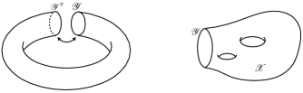
Figure 4: Left: construction of the mapping torus associated with a global transformation $\pi$. The two boundaries of the cylinder $\mathcal{Y}\times[0,1]$ are glued together modulo $\pi$. Right: the Euclidean spacetime $\mathcal{Y}$ is seen as the boundary of a $(D+1)$-dimensional manifolds with all the relevant mathematical structures on $\mathcal{Y}$ properly extended.

In page 2 we learned how perturbative anomalies on an even $D$-dimensional manifold $\mathcal{Y}$ are obtained from the variation of a $(D+1)$-dimensional Chern-Simons form, related to the index of a Dirac operator in $D+2$ dimensions. A similar structure exists for global anomalies Witten_global_grav where the central role is played by the $\eta$-invariant, defined as the regularized sum of the signs of the eigenvalues of the Dirac operator

$$\eta\equiv\Big{[}\sum_{\lambda_{i}\neq 0}\mbox{sign}(\lambda_{i})\Big{]}_{\rm reg}=\lim_{\epsilon\rightarrow 0^{+}}\sum_{\lambda_{i}\neq 0}{\lambda_{i}\over|\lambda_{i}|}e^{-\epsilon|\lambda_{i}|}.$$ (135)

The variation of the effective action under a global transformation $\pi$ is given in terms of the $\eta$-invariant of the associated mapping torus $\mathcal{T}_{\pi}\equiv(\mathcal{Y}\times S^{1})_{\pi}$. This is constructed from the cylinder $\mathcal{Y}\times[0,1]$ by identifying its boundaries modulo the transformation $\pi$, as shown on the left of fig. 4. For a Weyl fermion, the result is

$$\Delta_{\pi}\Gamma_{\rm eff}\equiv\Gamma_{\rm eff}^{\pi}-\Gamma_{\rm eff}={i\pi\over 2}\eta_{\mathcal{T}_{\pi}}.$$ (136)

The Atiyal-Patodi-Singer (APS) theorem relates this $\eta$-invariant to the index of the Dirac operator on a $(D+2)$-dimensional manifold $\mathcal{B}$ such that $\partial\mathcal{B}=\mathcal{T}_{\pi}$

$${1\over 2}\eta_{\mathcal{T}_{\pi}}=\mbox{index}_{\mathcal{B}}(iD\!\!\!\!\!/)-\int_{\mathcal{B}}[\widehat{A}(\mathcal{R})\mbox{ch}(\mathcal{F})]_{D+2},$$ (137)

where the second term on the right-hand side vanishes in the absence of perturbative anomalies.

The APS $\eta$-invariant is in fact the key to a whole new approach to anomalies building on the notion of anomaly inflow and with deep mathematical implications dai_freed ; df_cm ; df_hep . Let us take our Euclidean $D$-dimensional manifold of interest $\mathcal{Y}$ to be the boundary of some manifold $\mathcal{X}$ (see the right of fig. 4). In order to define fermions properly, we require the spin/pin structure on $\mathcal{Y}$ to be smoothly extended to $\mathcal{X}$. Moreover, boundary conditions for fermions on $\mathcal{Y}=\partial\mathcal{X}$ have to be carefully chosen so the Dirac operator on $\mathcal{X}$ is self-adjoint (see dai_freed ; df_cm ; df_hep for the technical details). Once all mathematical subtleties are properly handled, the partition function for a Weyl fermion on $\mathcal{Y}$ can be written as

$$Z\equiv e^{-\Gamma_{\rm eff}}=|\mbox{Pf}(iD\!\!\!\!\!/\,)|\exp\left(-{i\pi\over 2}\eta_{\mathcal{X}}\right)\exp\left(-2\pi i\int_{\mathcal{X}}I^{0}_{D+1}\right).$$ (138)

This expression is independent on changes on either the metric or the gauge field on $\mathcal{X}$ as far as these do not affect their values on $\mathcal{Y}$. This means that, despite appearances, it only depends on field theory data on the boundary.

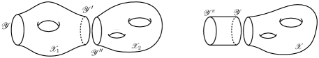
Figure 5: Left: gluing two surfaces together along their boundaries $\mathcal{Y}^{\prime}$ and $\mathcal{Y}^{\prime\prime}$. Right: global transformations are implemented by attaching to $\mathcal{Y}=\partial\mathcal{X}$ the appropriate mapping torus.

The fermion partition function (138) smoothly connects with the standard analysis of perturbative and global anomalies. For the first type, the $\eta$-invariant remains unchanged while the variation of the Chern-Simons form gives the known expression for the integrated anomaly. The partition function may also change under transformations not connected with the identity, and here is where the sewing properties of the $\eta$-invariant come in handy. Consider two manifolds $\mathcal{X}_{1}$ and $\mathcal{X}_{2}$ being glued together by their boundaries, as shown on the left of fig. 5. The $\eta$-invariant associated with the glued manifold $\mathcal{X}_{1}\sqcup\mathcal{X}_{2}$ is given by

$$e^{-{i\pi\over 2}\eta_{\mathcal{X}_{1}\sqcup\mathcal{X}_{2}}}=e^{-{i\pi\over 2}\eta_{\mathcal{X}_{1}}}e^{-{i\pi\over 2}\eta_{\mathcal{X}_{2}}}.$$ (139)

We can apply this relation to compute the change in the partition function (138) under a global transformation $\pi$, implemented by gluing the corresponding mapping torus to the boundary of $\mathcal{X}$ (see the right of fig. 5). Using eq. (139), we find

$${Z^{\pi}\over Z}=e^{-{i\pi\over 2}\eta_{\mathcal{T}_{\pi}}},$$ (140)

which reproduces the form of the global anomaly given in (136). In the previous discussion we assumed tacitly that $D$ is even and focused our attention on gauge and gravitational anomalies. For $D$ odd, the Chern-Simons term in the partition function is absent and the standard treatment of parity anomaly in terms of the $\eta$-invariant AGdPM is retrieved.

The phase in eq. (138) can be interpreted as the partition function of an “anomaly” topological field theory defined on $\mathcal{X}$ that includes fermions. An important question is whether there are ambiguities associated with the choice of the manifold $\mathcal{X}$, the so-called Dai-Freed anomalies. In fact, the consistency of the theory on $\mathcal{Y}$ requires then that the fermion partition function does not depend on the higher-dimensional manifold $\mathcal{X}$ used and therefore that it is free from Dai-Freed anomalies. Defining the partition function using two different manifolds $\mathcal{X}_{1}$ and $\mathcal{X}_{2}$ with $\mathcal{Y}=\partial\mathcal{X}_{1}=\partial\mathcal{X}_{2}$, this condition takes the form

$$1={Z_{1}\over Z_{2}}=e^{{i\pi\over 2}\eta_{\mathcal{X}_{1}\sqcup\overline{\mathcal{X}}_{2}}},$$ (141)

where $\mathcal{X}_{1}\sqcup\overline{\mathcal{X}}_{2}$ is the closed manifold resulting from gluing $\mathcal{X}_{1}$ and $\mathcal{X}_{2}$ along their common boundary and the bar indicates orientation reversal (the property $\eta_{\overline{\mathcal{X}}}=-\eta_{\mathcal{X}}$ was also used). Notice that $\mathcal{X}_{1}\sqcup\overline{\mathcal{X}}_{2}$ can be seen as the boundary of a $(D+2)$-dimensional manifold. Using the Stokes theorem together with $dI^{0}_{D+1}=I_{D+2}$, we find that the integral of the Chern-Simons term over the closed manifold gives an integer resulting in a trivial phase.

Equation (141) means that the cancellation of Dai-Freed anomalies is equivalent to the requirement that the higher-dimensional anomaly topological field theory is trivial. This condition comprises the absence of standard gauge and gravitational (perturbative and global) anomalies, but in fact goes much beyond. It includes a wider class of consistency conditions to be imposed on quantum field theories. This has found interesting application in string theory df_st , high-energy phenomenology df_hep , and the physics of the topological phases of matter df_cm .

But there are more interesting mathematics lurking behind all this. Two closed $D$-dimensional manifolds $\mathcal{Y}_{1}$ and $\mathcal{Y}_{2}$ are in the same equivalence bordism class if their disjoint union $\mathcal{Y}_{1}\sqcup\overline{\mathcal{Y}}_{2}$ is the boundary of some $(D+1)$-dimensional manifold. An example of this is illustrated on the left picture of fig. 5, where from $\mathcal{Y}\sqcup\mathcal{Y}^{\prime}=\partial\mathcal{X}_{1}$ we see that $\mathcal{Y}$ and $\overline{\mathcal{Y}}^{\prime}$ belong to the same bordism class. The discussion above indicates that the cancellation of Dai-Freed anomalies means that consistent fermion theories are invariant under bordisms. In other words, it does not matter what representative $\mathcal{X}$ within a bordism equivalence class we choose to define the theory.

This bordism invariance has led to a fascinating connection with category theory, one of the booming topics in contemporary mathematics (see categories_rev for a physicist-oriented review). To discuss just the rudiments of category theory and how they apply to the analysis of quantum field theory anomalies lies way beyond the scope of this brief overview. The reader can find a nice introduction to this topic in ref. monnier . It is in any case interesting how, since their diagrammatic inception in 1969 discovery , the subject of quantum field theory anomalies has provided a fertile ground for the application of new mathematics. It was from the late 1970s on AS that the beautiful and insightful connection with the index theorems emerged. This did not just clarify many features of anomalies already identified in the diagrammatic approach, such as their saturation at one loop, but also highlighted its very general nature independent of the technical details of the Feynman diagram computations where they were first identified. Although the categorial approach to anomalies is still very much under exploration, the expectation exists that it could lead to a deepening of our understanding of quantum fields in some way comparable to what was achieved by the implementation of differential geometry techniques.

References

- (1) L. Álvarez-Gaumé, M. Á. Vázquez-Mozo, An Invitation to Quantum Field Theory, Springer, 2012.
-
(2)
L. Álvarez-Gaumé,
An Introduction to Anomalies, in
“Fundamental
Problems of Gauge Field Theory”, Plenum Press,
1985.
R. A. Bertlmann, Anomalies in Quantum Field Theory, Oxford University Press, 1996.
K. Fujikawa and H. Suzuki, Path Integrals and Quantum Anomalies, Oxford University Press, 2004.
A. Bilal, Lectures on Anomalies, arXiv:0802.0634 [hep-th]. - (3) J. A. Harvey, TASI Lectures on Anomalies, arXiv:hep-th/0509097 [hep-th].
- (4) W. A. Bardeen and B. Zumino, Consistent and Covariant Anomalies in Gauge and Gravitational Theories, Nucl. Phys. B 244 (1984) 421.
- (5) L. Álvarez-Gaumé and P. Ginsparg, The Structure of Gauge and Gravitational Anomalies, Annals Phys. 161 (1985) 423.
- (6) M. Nakahara, Geometry, Topology and Physics (2nd edition), Taylor & Francis, 2003.
-
(7)
B. Zumino,
Chiral anomalies and differential geometry,
in “Relativity, groups and topology”, Elsevier (1983).
M. F. Atiyah and I. M. Singer, Dirac Operators Coupled to Vector Potentials, Proc. Nat. Acad. Sci. 81 (1984) 2597.
B. Zumino, Y. S. Wu and A. Zee, Chiral Anomalies, Higher Dimensions, and Differential Geometry, Nucl. Phys. B 239 (1984) 477. - (8) L. Álvarez-Gaumé and P. Ginsparg, The Topological Meaning of Nonabelian Anomalies, Nucl. Phys. B 243 (1984) 449.
- (9) L. Álvarez-Gaumé and E. Witten, Gravitational Anomalies, Nucl. Phys. B 234 (1984) 269.
- (10) M. B. Green and J. H. Schwarz, Anomaly Cancellation in Supersymmetric D=10 Gauge Theory and Superstring Theory, Phys. Lett. B 149 (1984) 117.
- (11) M. B. Green and J. H. Schwarz, The Hexagon Gauge Anomaly in Type I Superstring Theory, Nucl. Phys. B 255 (1985) 93.
-
(12)
L. Álvarez-Gaumé and M. Á. Vázquez-Mozo, Topics in String Theory and Quantum
Gravity, in: “Gravitation and Quantizations”, Proceedings of the 1992 Les Houches
Summer School, Elsevier 1995 [hep-th/9212006].
J. Polchinski, String Theory vols. I & II, Cambridge 1998.
K. Becker, M. Becker and J. H. Schwarz, String Theory and M-Theory: A Modern Introduction, Cambridge 2006.
L. E. Ibáñez and Á. M. Uranga, String Theory and Particle Physics: An Introduction to String Phenomenology, Cambridge 2012.
E. Kiritsis, String Theory in a Nutshell, Princeton 2019. - (13) C. V. Johnson, D-branes, Cambridge 2003.
- (14) M. B. Green, J. H. Schwarz and E. Witten, Superstring Theory vols I & II, Cambridge 1987.
- (15) J. Polchinski and Y. Cai, Consistency of Open Superstring Theories, Nucl. Phys. B 296 (1988) 91.
- (16) M. B. Green and J. H. Schwarz, Infinity Cancellations in SO(32) Superstring Theory, Phys. Lett. B 151 (1985) 21.
-
(17)
A. H. Chamseddine,
Interacting Supergravity in Ten-Dimensions: The Role of the Six-Index Gauge Field,
Phys. Rev. D 24 (1981) 3065.
E. Bergshoeff, M. de Roo, B. de Wit and P. van Nieuwenhuizen, Ten-Dimensional Maxwell-Einstein Supergravity, Its Currents, and the Issue of Its Auxiliary Fields, Nucl. Phys. B 195 (1982) 97. - (18) G. F. Chapline and N. S. Manton, Unification of Yang-Mills Theory and Supergravity in Ten-Dimensions, Phys. Lett. B 120 (1983) 105.
- (19) J. Wess and B. Zumino, Consequences of anomalous Ward identities, Phys. Lett. B 37 (1971) 95.
- (20) M. Hayashi, N. Kawamoto, T. Kuramoto and K. Shigemoto, Gravitational Anomaly Cancellation in Type I Superstring Theory, Nucl. Phys. B 296 (1988) 373.
-
(21)
D. J. Gross, J. A. Harvey, E. J. Martinec and R. Rohm,
Heterotic String Theory. 1. The Free Heterotic String,
Nucl. Phys. B 256 (1985) 253.
D. J. Gross, J. A. Harvey, E. J. Martinec and R. Rohm, Heterotic String Theory. 2. The Interacting Heterotic String, Nucl. Phys. B 267 (1986) 75. - (22) M. Hayashi, N. Kawamoto, T. Kuramoto and K. Shigemoto, Modular Invariance and Gravitational Anomaly in Type II Superstring Theory, Nucl. Phys. B 294 (1987) 459.
-
(23)
A. N. Schellekens and N. P. Warner,
Anomalies and Modular Invariance in String Theory,
Phys. Lett. B 177
(1986) 317.
H. Suzuki and A. Sugamoto, Role of Modular Invariance in Evaluation of Gauge and Gravitational Anomalies in the Heterotic String, Phys. Rev. Lett. 57 (1986) 1665.
W. Lerche, B. E. W. Nilsson and A. N. Schellekens, Heterotic String-Loop Calculation of the Anomaly Cancelling Term, Nucl. Phys. B 289 (1987) 609.
D. J. Gross and P. F. Mende, Modular Subgroups, Odd Spin Structures and Gauge Invariance in the Heterotic String, Nucl. Phys. B 291 (1987) 653.
D. Kutasov, Modular Invariance, Chiral Anomalies and Contact Terms, Nucl. Phys. B 307 (1988) 417.
W. Lerche, A. N. Schellekens and N. P. Warner, Lattices and Strings, Phys. Rept. 177 (1989) 1. - (24) L. Álvarez-Gaumé, P. H. Ginsparg, G. W. Moore and C. Vafa, An Heterotic String, Phys. Lett. B 171 (1986) 155.
- (25) S. Sugimoto, Anomaly cancellations in type I D-9-anti-D-9 system and the USp(32) string theory, Prog. Theor. Phys. 102 (1999) 685 [arXiv:hep-th/9905159 [hep-th]].
- (26) Q. Bonnefoy and E. Dudas, Axions and anomalous U(1)’s, Int. J. Mod. Phys. A 33 (2018) 1845001 [arXiv:1809.08256 [hep-ph]].
- (27) J. Mañes, R. Stora and B. Zumino, Algebraic Study of Chiral Anomalies, Commun. Math. Phys. 102 (1985) 157.
- (28) J. L. Mañes, E. Megías, M. Valle and M. Á. Vázquez-Mozo, Non-Abelian Anomalous (Super)Fluids in Thermal Equilibrium from Differential Geometry, JHEP 11 (2018) 076 [arXiv:1806.07647 [hep-th]].
- (29) C. G. Callan and J. A. Harvey, Anomalies and Fermion Zero Modes on Strings and Domain Walls, Nucl. Phys. B 250 (1985) 427.
- (30) J. D. Blum and J. A. Harvey, Anomaly inflow for gauge defects, Nucl. Phys. B 416 (1994) 119 [arXiv:hep-th/9310035 [hep-th]].
- (31) J. Goldstone and F. Wilczek, Fractional Quantum Numbers on Solitons, Phys. Rev. Lett. 47 (1981) 986.
- (32) S. G. Naculich, Axionic Strings: Covariant Anomalies and Bosonization of Chiral Zero Modes, Nucl. Phys. B 296 (1988) 837.
- (33) J. Polchinski, Dirichlet Branes and Ramond-Ramond charges, Phys. Rev. Lett. 75 (1995) 4724 [arXiv:hep-th/9510017 [hep-th]].
- (34) M. J. Duff, R. R. Khuri and J. X. Lu, String solitons, Phys. Rept. 259 (1995) 213 [arXiv:hep-th/9412184 [hep-th]].
- (35) M. B. Green, J. A. Harvey and G. W. Moore, I-brane inflow and anomalous couplings on d-branes, Class. Quant. Grav. 14 (1997) 47 [arXiv:hep-th/9605033 [hep-th]].
- (36) Y. K. E. Cheung and Z. Yin, Anomalies, branes, and currents, Nucl. Phys. B 517 (1998) 69 [arXiv:hep-th/9710206 [hep-th]].
- (37) R. J. Szabo, An Introduction to String Theory and D-brane Dynamics (2nd edition), Imperial College Press 2011.
- (38) N. Seiberg, Notes on theories with 16 supercharges, Nucl. Phys. B Proc. Suppl. 67 (1998) 158 [arXiv:hep-th/9705117 [hep-th]].
- (39) C. Nash, Topology and Quantum Field Theory, Academic Press 1991.
- (40) J. F. Morales, C. A. Scrucca and M. Serone, Anomalous couplings for D-branes and O-planes, Nucl. Phys. B 552 (1999) 291 [arXiv:hep-th/9812071 [hep-th]].
- (41) C. A. Scrucca and M. Serone, Anomalies and inflow on D-branes and O-planes, Nucl. Phys. B 556 (1999) 197 [arXiv:hep-th/9903145 [hep-th]].
- (42) E. Witten, An SU(2) Anomaly, Phys. Lett. B 117 (1982) 324.
- (43) E. Witten, Global Gravitational Anomalies, Commun. Math. Phys. 100 (1985) 197.
-
(44)
X. Dai and D. S. Freed,
invariants and determinant lines,
J. Math. Phys. 35 (1994) 5155
[arXiv:hep-th/9405012 [hep-th]].
E. Witten and K. Yonekura, Anomaly Inflow and the -Invariant, in: “Memorial Volume for Shoucheng Zhang”, World Scientific 2021 [arXiv:1909.08775 [hep-th]]. -
(45)
E. Witten,
Fermion path integrals and topological phases,
Rev. Mod. Phys. 88 (2016) 035001
[arXiv:1508.04715 [cond-mat.mes-hall]].
E. Witten, The ”parity” anomaly on an unorientable manifold, Phys. Rev. B 94 (2016) 195150 [arXiv:1605.02391 [hep-th]].
K. Yonekura, Dai-Freed theorem and topological phases of matter, JHEP 09 (2016), 022 [arXiv:1607.01873 [hep-th]]. - (46) I. García-Etxebarria and M. Montero, Dai-Freed anomalies in particle physics, JHEP 08 (2019) 003 [arXiv:1808.00009 [hep-th]].
- (47) L. Álvarez-Gaumé, S. Della Pietra and G. Moore, Anomalies and Odd Dimensions, Annals Phys. 163 (1985) 288.
- (48) D. S. Freed and E. Witten, Anomalies in string theory with D-branes, Asian J. Math. 3 (1999) 819 [arXiv:hep-th/9907189 [hep-th]].
- (49) B. Coecke, É. O. Paquette, Categories for the Practicing Physicist, in: “New Structures in Physics” ed. B. Coecke, Springer 2011.
- (50) S. Monnier, A Modern Point of View on Anomalies, Fortsch. Phys. 67 (2019) 1910012 [arXiv:1903.02828 [hep-th]].
-
(51)
S. L. Adler,
Axial vector vertex in spinor electrodynamics,
Phys. Rev. 177 (1969) 2426.
J. S. Bell and R. Jackiw, A PCAC puzzle: in the model, Nuovo Cim. A 60 (1969) 47. -
(52)
N. K. Nielsen and B. Schroer,
Axial Anomaly and Atiyah-Singer Theorem,
Nucl. Phys. B 127 (1977) 493.
N. K. Nielsen, H. Römer and B. Schroer, Classical Anomalies and Local Version of the Atiyah-Singer Theorem, Phys. Lett. B 70 (1977) 445.
K. Fujikawa, Path Integral Measure for Gauge Invariant Fermion Theories, Phys. Rev. Lett. 42 (1979) 1195.
K. Fujikawa, Path Integral for Gauge Theories with Fermions, Phys. Rev. D 21 (1980) 2848.